Tropospheric Modeling

S. I. Gutman

Chief, GPS-Met Observing Systems Section NOAA Earth System Research Laboratory

Boulder, Colorado USA

2

Introduction

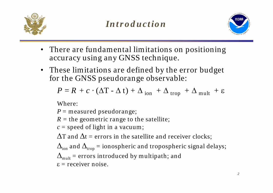
• There are fundamental limitations on positioning accuracy using any GNSS technique.

• These limitations are defined by the error budget for the GNSS pseudorange observable:

P = R + c · (ΔT - Δ t) + Δ ion + Δ trop + Δ mult + ε

Where:P = measured pseudorange; R = the geometric range to the satellite; c = speed of light in a vacuum;

ΔT and Δt = errors in the satellite and receiver clocks;

Δion and Δtrop = ionospheric and tropospheric signal delays; -

Δmult = errors introduced by multipath; and ε = receiver noise.

3

Introduction

• GNSS positioning accuracy ultimately depends on how well all of the potential sources of error can be measured, estimated and/or eliminated.

• This presentation will focus on:

1. GNSS signal delays caused by the Earth’s atmosphere, concentrating on the neutral (non-dispersive) region called the troposphere.

2. Common techniques to estimate and minimize the impact of tropospheric delays on GNSS accuracy.

3. Alternative approach to this problem.

4. Opportunities for international collaboration.

4

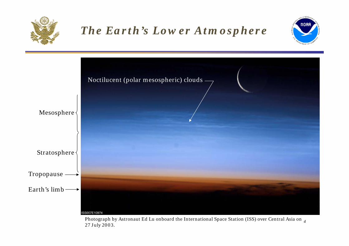
The Earth’s Lower Atmosphere

Tropopause

Earth’s limb

Stratosphere

Noctilucent (polar mesospheric) clouds

Mesosphere

Photograph by Astronaut Ed Lu onboard the International Space Station (ISS) over Central Asia on 27 July 2003.

5

Atmospheric Signal Delays

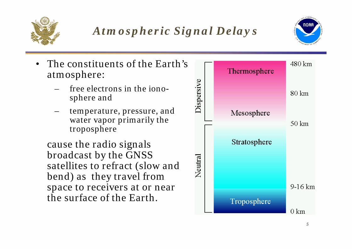
• The constituents of the Earth’s atmosphere:

– free electrons in the iono-sphere and

– temperature, pressure, and water vapor primarily the troposphere

cause the radio signals broadcast by the GNSS satellites to refract (slow and bend) as they travel from space to receivers at or near the surface of the Earth.

6

Atmospheric Signal Delays

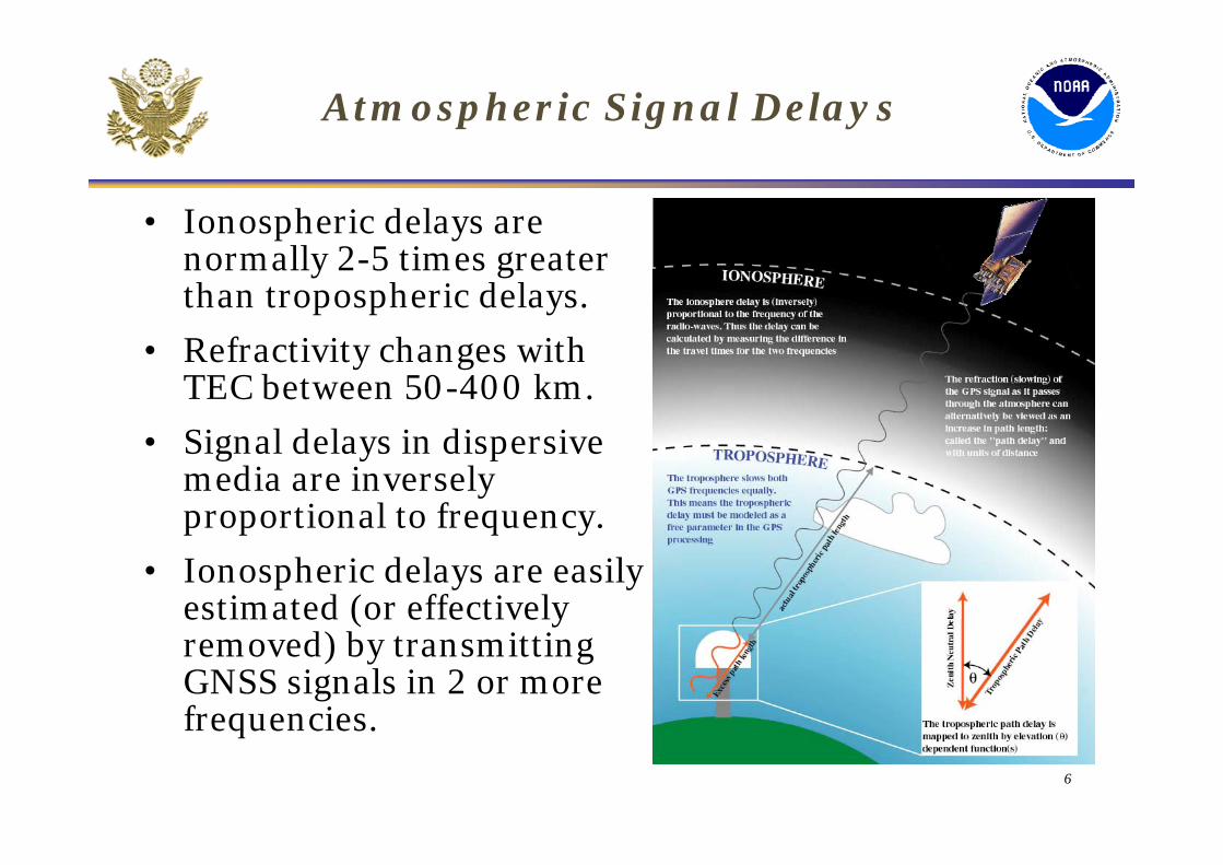
• Ionospheric delays are normally 2-5 times greater than tropospheric delays.

• Refractivity changes with TEC between 50-400 km.

• Signal delays in dispersive media are inversely proportional to frequency.

• Ionospheric delays are easily estimated (or effectively removed) by transmitting GNSS signals in 2 or more frequencies.

7

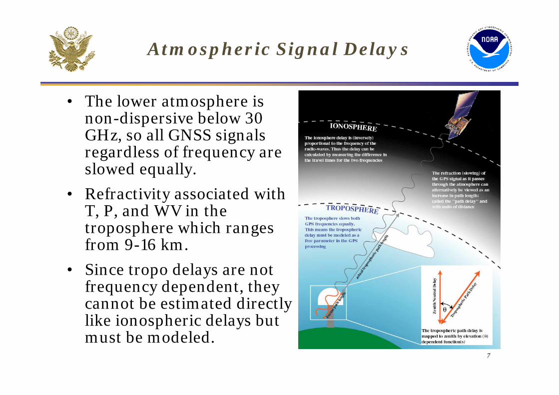
• The lower atmosphere is non-dispersive below 30 GHz, so all GNSS signals regardless of frequency are slowed equally.

• Refractivity associated with T, P, and WV in the troposphere which ranges from 9-16 km.

• Since tropo delays are not frequency dependent, they cannot be estimated directly like ionospheric delays but must be modeled.

Atmospheric Signal Delays

8

Atmospheric Signal Delays

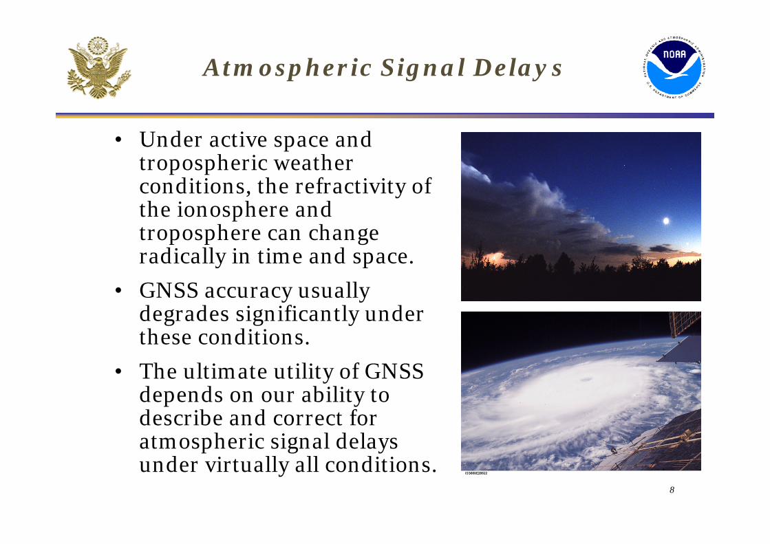
• Under active space and tropospheric weather conditions, the refractivity of the ionosphere and troposphere can change radically in time and space.

• GNSS accuracy usually degrades significantly under these conditions.

• The ultimate utility of GNSS depends on our ability to describe and correct for atmospheric signal delays under virtually all conditions.

9

Correcting Tropospheric Errors

• Commonly Used Strategies– Ignore the tropospheric delay

– Estimate the tropospheric delay from surface meteorological observations

– Predict the tropospheric delay from empirically-derived signal delay climatology

– Use additional information provided by ground and space-based augmentations

– Estimate directly from carrier phase observables.

• Different strategies are appropriate for different applications.

• Positioning accuracy is not the only criterion for selecting a error mitigation strategy.

10

Commonly Used Strategies

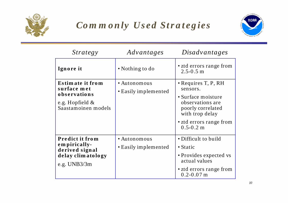
• Requires T, P, RH sensors.

• Surface moisture observations are poorly correlated with trop delay

• ztd errors range from 0.5-0.2 m

• Autonomous

• Easily implemented

Estimate it from surface met observations

e.g. Hopfield & Saastamoinen models

• Difficult to build

• Static

• Provides expected vsactual values

• ztd errors range from 0.2-0.07 m

• Autonomous

• Easily implemented

Predict it from empirically-derived signal delay climatology

e.g. UNB3/3m

• ztd errors range from 2.5-0.5 m• Nothing to doIgnore it

Strategy Advantages Disadvantages

11

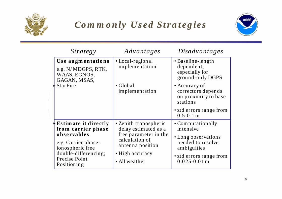
Commonly Used Strategies

• Computationally intensive

• Long observations needed to resolve ambiguities

• ztd errors range from 0.025-0.01 m

• Zenith tropospheric delay estimated as a free parameter in the calculation of antenna position

• High accuracy

• All weather

Estimate it directly from carrier phase observables

e.g. Carrier phase-ionospheric free double-differencing; Precise Point Positioning

• Baseline-length dependent, especially for ground-only DGPS

• Accuracy of correctors depends on proximity to base stations

• ztd errors range from 0.5-0.1 m

• Local-regional implementation

• Global implementation

Use augmentations

e.g. N/MDGPS, RTK, WAAS, EGNOS, GAGAN, MSAS, StarFire

Strategy Advantages Disadvantages

12

Alternative Approach

• Assimilate meteorological data into numerical weather prediction (NWP) models.

• Invert analyses and short-term predictions to provide real-time tropospheric signal delay estimates.

• For all end users, NWP-derived signal delay information is independent of their GNSS range or carrier phase observations.

• It is now possible to provide the following signal delay estimates at any point in the model domain:

– Zenith hydrostatic delay (zhd)

– Zenith wet delay (zwd)

– Horizontal gradients in zhd and zwd.

13

• Largest errors in NWP come from:– Limitations in our ability to describe water vapor

variability in time and space

– Mismodeling 4-d moisture structure.

• Largest errors in GNSS height measurements come from tropospheric delay errors caused by water vapor variability.

• Significant improvements in weather forecast accuracy in U.S., Canada and Europe result from assimilation of GNSS signal delays into NWP models.

• We expect similar improvements in GNSS accuracy using this approach.

Comments on Alternative Approach

14

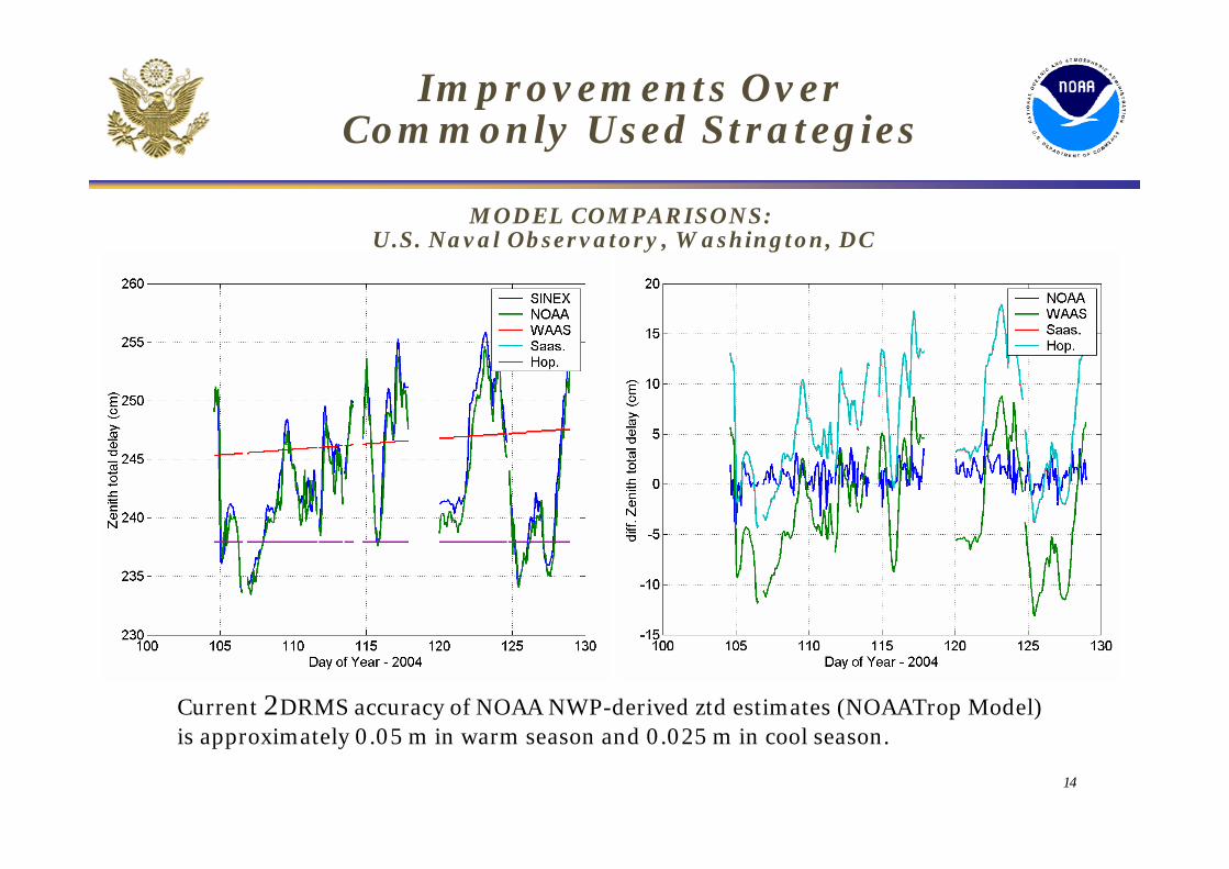
Improvements Over Commonly Used Strategies

MODEL COMPARISONS:U.S. Naval Observatory, Washington, DC

Current 2DRMS accuracy of NOAA NWP-derived ztd estimates (NOAATrop Model) is approximately 0.05 m in warm season and 0.025 m in cool season.

15

Reported Improvements in GNSS Positioning Accuracy

• University of Calgary:– 10-40% improvement in Northeast U.S. baselines

depending on surveying approach (e.g. using single or multiple base stations).

• University of Southern Mississippi:– 8.9% improvement in South East U.S. (Gulf Coast)

during warm season.

– 16.3% improvement in North Central U.S. (Great Lakes) during warm season.

– 25.2% improvement in South West U.S. (So. California) during warm season.

16

Reported Improvements in GNSS Positioning Accuracy

• University of California Scripps Institution:– 10% improvement in accuracy

– 15% improvement in precision

– model reduces correlation between zenith delay, multipath, and vertical position at all timescales

– but improvements diminishes with time.

• Problems manifest themselves in different ways:– In areas of high relief and low humidity, RMS errors are

associated with increased bias. This suggests that errors are related to the spatial resolution of the model.

– In areas of low relief and high humidity, RMS errors are associated with increased standard deviation. This suggests that the problem is related to our ability to capture the variability of moisture.

17

Opportunities for International Collaboration

• Expand NRT GNSS observations:– In poorly observed regions of the planet

– In areas prone to natural disasters.

• Expected results:– Improved air, sea and land transportation safety

– Improved global weather prediction

– Improved climate monitoring

– Improved monitoring of sea level

– Real-time monitoring of active faults, volcanoes and other geological hazards

– Improved lead-time for tsunami warnings

– More effective use of satellite data through global calibration and validation