Policy Gradient Methods - Robot Learningrll.berkeley.edu/deeprlcourse/docs/lec2.pdf1.Make the good...

Policy Gradient Methods

February 13, 2017

Policy Optimization Problems

maximizeπ

Eπ [expression]

I Fixed-horizon episodic:∑T−1

t=0 rt

I Average-cost: limT→∞1T

∑T−1t=0 rt

I Infinite-horizon discounted:∑∞

t=0 γtrt

I Variable-length undiscounted:∑Tterminal−1

t=0 rtI Infinite-horizon undiscounted:

∑∞t=0 rt

Episodic Setting

μ0

a0

s0 s1

a1 aT-1

sT

π

P

Agent

r0 r1 rT-1

Environment

s2

Objective:

maximize η(π), where

η(π) = E [r0 + r1 + · · ·+ rT−1 | π]

Parameterized Policies

I A family of policies indexed by parameter vector θ ∈ Rd

I Deterministic: a = π(s, θ)I Stochastic: π(a | s, θ)

I Analogous to classification or regression with input s, output a.I Discrete action space: network outputs vector of probabilitiesI Continuous action space: network outputs mean and diagonal covariance of

Gaussian

Policy Gradient Methods: Overview

Problem:

maximizeE [R | πθ]

Intuitions: collect a bunch of trajectories, and ...

1. Make the good trajectories more probable1

2. Make the good actions more probable

3. Push the actions towards good actions (DPG2, SVG3)

1R. J. Williams. “Simple statistical gradient-following algorithms for connectionist reinforcement learning”. Machine learning (1992);R. S. Sutton, D. McAllester, S. Singh, and Y. Mansour. “Policy gradient methods for reinforcement learning with function approximation”. NIPS.MIT Press, 2000.

2D. Silver, G. Lever, N. Heess, T. Degris, D. Wierstra, et al. “Deterministic Policy Gradient Algorithms”. ICML. 2014.

3N. Heess, G. Wayne, D. Silver, T. Lillicrap, Y. Tassa, et al. “Learning Continuous Control Policies by Stochastic Value Gradients”. arXivpreprint arXiv:1510.09142 (2015).

Derivation via Importance Sampling

Alternative Derivation Using Importance Sampling4

Ex∼θ [f (x)] = Ex∼θold

[p(x | θ)

p(x | θold)f (x)

]∇θEx∼θ [f (x)] = Ex∼θold

[∇θp(x | θ)

p(x | θold)f (x)

]∇θEx∼θ [f (x)]

∣∣θ=θold

= Ex∼θold

[∇θp(x | θ)

∣∣θ=θold

p(x | θold)f (x)

]= Ex∼θold

[∇θ log p(x | θ)

∣∣θ=θold

f (x)]

4T. Jie and P. Abbeel. “On a connection between importance sampling and the likelihood ratio policy gradient”. Advances in Neural InformationProcessing Systems. 2010, pp. 1000–1008.

Score Function Gradient Estimator: Intuition

gi = f (xi)∇θ log p(xi | θ)

I Let’s say that f (x) measures how good the sample x is.

I Moving in the direction gi pushes up the logprob of thesample, in proportion to how good it is

I Valid even if f (x) is discontinuous, and unknown, or samplespace (containing x) is a discrete set

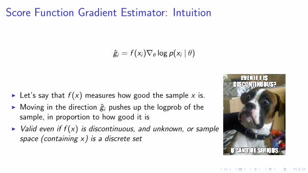
Score Function Gradient Estimator: Intuition

gi = f (xi)∇θ log p(xi | θ)

Score Function Gradient Estimator for PoliciesI Now random variable x is a whole trajectory τ = (s0, a0, r0, s1, a1, r1, . . . , sT−1, aT−1, rT−1, sT )

∇θEτ [R(τ)] = Eτ [∇θ log p(τ | θ)R(τ)]

I Just need to write out p(τ | θ):

p(τ | θ) = µ(s0)

T−1∏t=0

[π(at | st , θ)P(st+1, rt | st , at)]

log p(τ | θ) = log µ(s0) +

T−1∑t=0

[log π(at | st , θ) + log P(st+1, rt | st , at)]

∇θ log p(τ | θ) = ∇θT−1∑t=0

log π(at | st , θ)

∇θEτ [R] = Eτ

[R∇θ

T−1∑t=0

log π(at | st , θ)

]

I Interpretation: using good trajectories (high R) as supervised examples in classification / regression

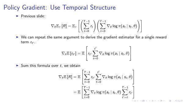
Policy Gradient: Use Temporal StructureI Previous slide:

∇θEτ [R] = Eτ

[(T−1∑t=0

rt

)(T−1∑t=0

∇θ log π(at | st , θ)

)]I We can repeat the same argument to derive the gradient estimator for a single reward

term rt′ .

∇θE [rt′ ] = E

rt′ t′∑t=0


I Sum this formula over t, we obtain

∇θE [R] = E

T−1∑t=0

rt′t′∑t=0


= E

[T−1∑t=0

∇θ log π(at | st , θ)T−1∑t′=t

rt′

]

Policy Gradient: Introduce Baseline

I Further reduce variance by introducing a baseline b(s)

∇θEτ [R] = Eτ

[T−1∑t=0


(T−1∑t′=t

rt′ − b(st)

)]

I For any choice of b, gradient estimator is unbiased.

I Near optimal choice is expected return,b(st) ≈ E [rt + rt+1 + rt+2 + · · ·+ rT−1]

I Interpretation: increase logprob of action at proportionally to how muchreturns

∑T−1t′=t rt′ are better than expected

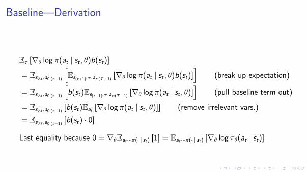
Baseline—Derivation

Eτ [∇θ log π(at | st , θ)b(st)]

= Es0:t ,a0:(t−1)

[Es(t+1):T ,at:(T−1)

[∇θ log π(at | st , θ)b(st)]]

(break up expectation)

= Es0:t ,a0:(t−1)

[b(st)Es(t+1):T ,at:(T−1)

[∇θ log π(at | st , θ)]]

(pull baseline term out)

= Es0:t ,a0:(t−1)[b(st)Eat [∇θ log π(at | st , θ)]] (remove irrelevant vars.)

= Es0:t ,a0:(t−1)[b(st) · 0]

Last equality because 0 = ∇θEat∼π(· | st) [1] = Eat∼π(· | st) [∇θ log πθ(at | st)]

Discounts for Variance Reduction

I Introduce discount factor γ, which ignores delayed effects between actionsand rewards

∇θEτ [R] ≈ Eτ

[T−1∑t=0


(T−1∑t′=t

γt′−trt′ − b(st)

)]

I Now, we want b(st) ≈ E[rt + γrt+1 + γ2rt+2 + · · ·+ γT−1−trT−1

]

“Vanilla” Policy Gradient Algorithm

Initialize policy parameter θ, baseline bfor iteration=1, 2, . . . do

Collect a set of trajectories by executing the current policyAt each timestep in each trajectory, compute

the return Rt =∑T−1

t′=t γt′−trt′ , and

the advantage estimate At = Rt − b(st).Re-fit the baseline, by minimizing ‖b(st)− Rt‖2,

summed over all trajectories and timesteps.Update the policy, using a policy gradient estimate g ,

which is a sum of terms ∇θ log π(at | st , θ)At .(Plug g into SGD or ADAM)

end for

Practical Implementation with Autodiff

I Usual formula∑

t ∇θ log π(at | st ; θ)At is inefficient—want to batch data

I Define “surrogate” function using data from currecnt batch

L(θ) =∑t

log π(at | st ; θ)At

I Then policy gradient estimator g = ∇θL(θ)

I Can also include value function fit error

L(θ) =∑t

(log π(at | st ; θ)At − ‖V (st)− Rt‖2

)

Value Functions

Qπ,γ(s, a) = Eπ[r0 + γr1 + γ2r2 + . . . | s0 = s, a0 = a

]Called Q-function or state-action-value function

V π,γ(s) = Eπ[r0 + γr1 + γ2r2 + . . . | s0 = s

]= Ea∼π [Qπ,γ(s, a)]

Called state-value function

Aπ,γ(s, a) = Qπ,γ(s, a)− V π,γ(s)

Called advantage function

Policy Gradient Formulas with Value FunctionsI Recall:

∇θEτ [R] = Eτ

[T−1∑t=0


(T−1∑t′=t

rt′ − b(st)

)]

≈ Eτ

[T−1∑t=0


(T−1∑t′=t

γt′−t rt′ − b(st)

)]

I Using value functions

∇θEτ [R] = Eτ

[T−1∑t=0

∇θ log π(at | st , θ)Qπ(st , at)

]

= Eτ

[T−1∑t=0

∇θ log π(at | st , θ)Aπ(st , at)

]

≈ Eτ

[T−1∑t=0

∇θ log π(at | st , θ)Aπ,γ(st , at)

]

I Can plug in “advantage estimator” A for Aπ,γ

I Advantage estimators have the form Return− V (s)

Value Functions in the Future

I Baseline accounts for and removes the effect of past actions

I Can also use the value function to estimate future rewards

R(1)t = rt + γV (st+1) cut off at one timestep

R(2)t = rt + γrt+1 + γ2V (st+2) cut off at two timesteps

. . .

R(∞)t = rt + γrt+1 + γ2rt+2 + . . . ∞ timesteps (no V )

Value Functions in the Future

I Subtracting out baselines, we get advantage estimators

A(1)t = rt + γV (st+1)−V (st)

A(2)t = rt + rt+1 + γ2V (st+2)−V (st)

. . .

A(∞)t = rt + γrt+1 + γ2rt+2 + . . .−V (st)

I A(1)t has low variance but high bias, A

(∞)t has high variance but low bias.

I Using intermediate k (say, 20) gives an intermediate amount of bias and variance

Discounts: Connection to MPC

I MPC:

maximizea

Q∗,T (s, a) ≈ maximizea

Q∗,γ(s, a)

I Discounted policy gradient

Ea∼π [Qπ,γ(s, a)∇θ log π(a | s; θ)] = 0 when a ∈ arg maxQπ,γ(s, a)

Application: Robot Locomotion

Finite-Horizon Methods: Advantage Actor-Critic

I A2C / A3C uses this fixed-horizon advantage estimator. (NOTE: “async” is onlyfor speed, doesn’t improve performance)

I Pseudocode

for iteration=1, 2, . . . doAgent acts for T timesteps (e.g., T = 20),For each timestep t, compute

Rt = rt + γrt+1 + · · ·+ γT−t+1rT−1 + γT−tV (st)

At = Rt − V (st)

Rt is target value function, in regression problemAt is estimated advantage function

Compute loss gradient g = ∇θ

∑Tt=1

[− log πθ(at | st)At + c(V (s)− Rt)

2]

g is plugged into a stochastic gradient descent variant, e.g., Adam.end for

V. Mnih, A. P. Badia, M. Mirza, A. Graves, T. P. Lillicrap, et al. “Asynchronous methods for deep reinforcement learning”. (2016)

A3C Video

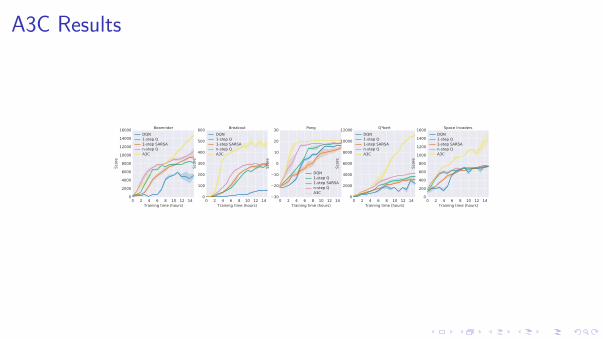
A3C Results

0 2 4 6 8 10 12 14Training time (hours)

0

2000

4000

6000

8000

10000

12000

14000

16000

Sco

re

Beamrider

DQN1-step Q1-step SARSAn-step QA3C


0

100

200

300

400

500

600

Sco

re

Breakout



30

20

10

0

10

20

30

Sco

re

Pong



0

2000

4000

6000

8000

10000

12000

Sco

re

Q*bert



0

200

400

600

800

1000

1200

1400

1600

Sco

re

Space Invaders


Further Reading

I A nice intuitive explanation of policy gradients:http://karpathy.github.io/2016/05/31/rl/

I R. J. Williams. “Simple statistical gradient-following algorithms forconnectionist reinforcement learning”. Machine learning (1992);R. S. Sutton, D. McAllester, S. Singh, and Y. Mansour. “Policy gradientmethods for reinforcement learning with function approximation”. NIPS.MIT Press, 2000

I My thesis has a decent self-contained introduction to policy gradientmethods: http://joschu.net/docs/thesis.pdf

I A3C paper: V. Mnih, A. P. Badia, M. Mirza, A. Graves, T. P. Lillicrap, et al.“Asynchronous methods for deep reinforcement learning”. (2016)

http://karpathy.github.io/2016/05/31/rl/

http://joschu.net/docs/thesis.pdf

Policy Gradient Methods - Robot Learningrll.berkeley.edu/deeprlcourse/docs/lec2.pdf1.Make the good...

Documents

Transcript of Policy Gradient Methods - Robot Learningrll.berkeley.edu/deeprlcourse/docs/lec2.pdf1.Make the good...