Physics 215 Solution Set 3 Winter 2018

1. Consider the one-dimensional problem of a particle moving in a delta-function potential:

V (x) = −Aδ(x) .

(a) Solve for the bound state energies and wave functions. Consider the cases A > 0 andA < 0 separately.

The time-independent Schrodinger equation for this problem is

− ~2

2m

d2ψ

dx2− Aδ(x)ψ(x) = Eψ(x) . (1)

Integrating this equation from x = −ǫ to x = ǫ, where ǫ > 0 is a positive infinitesimalquantity,

− ~2

2m

[

ψ′(ǫ)− ψ′(−ǫ)]

− Aψ(0) = E

∫ ǫ

−ǫ

ψ(x) dx .

where ψ′ ≡ dψ/dx. We require that ψ(x) is continuous at x = 0. If this were not truethen dψ/dx would behave like a delta function near x = 0 and d2ψ/dx2 would behave liethe derivative of a delta function.1 Such behavior is not compatible with eq. (1). Hence, itfollows that

∫ ǫ

−ǫ

ψ(x) dx ≃ ψ(0)

∫ ǫ

−ǫ

dx = 2ǫψ(0) ,

which vanishes in the limit of ǫ→ 0. We conclude that

limǫ→0

[

ψ′(ǫ)− ψ′(−ǫ)]

= −2mA

~2ψ(0) . (2)

That is, dψ/dx is not continuous at x = 0; its discontinuity is determined by eq. (2).

To solve for the bound state energies, we solve eq. (1) for x 6= 0. In this case, we can setδ(x) = 0. Normalizable energy eigenstates exist if and only if E < 0 and A > 0. That is, wesolve the differential equation,

− ~2

2m

d2ψ

dx2+ |E|ψ(x) = 0 , for x 6= 0,

where E = −|E|, under the assumption that limx→±∞ ψ(x) = 0. The solution to thisequation after imposing the boundary conditions at x = ±∞ is

ψ(x) =

Ne−αx , for x > 0,

Neαx , for x < 0,

1Recall that dΘ(x)/dx = δ(x), where Θ(x) is the Heavyside step function.

1

where N is a normalization constant, and

α ≡√

2m|E|~2

. (3)

Note that the sign of α (which is positive) is determined since limx→±∞ ψ(x) = 0.

The energy eigenvalues are determined by imposing eq. (2). Noting that N = ψ(0),eq. (2) yields

−2αN = −2mAN

~2,

which implies that

α =mA

~2. (4)

Note that we must require that A > 0 in order that bound state solutions exist, since A < 0is incompatible with the requirement that α > 0. Finally, inserting eq. (3) into eq. (4) yields

E = −|E| = −mA2

2~2.

That is, there is precisely one bound state. The corresponding energy eigenfunction is

ψE(x) =

(

mA

~2

)1/2

e−mA|x|/~2 , (5)

where we have determined that the normalization constant is N =√

mA/~2 by requiringthat

∫ ∞

−∞

|ψE(x)|2dx = 1 .

The normalization condition yields

1

|N |2 =

∫ ∞

−∞

e−2α|x| dx = 2

∫ ∞

0

e−2α|x| dx = − 1

αe−2α|x|

∣

∣

∣

∣

∞

0

=1

α=

~2

mA,

after using eq. (4). The phase of N is conventionally taken to be unity, in which caseN = (mA/~2)1/2, as indicated in eq. (5).

(b) In the case of A > 0, consider a scattering process where the incident wave entersfrom the left with E = ~

2k2/(2m) > 0 (where E is the energy eigenvalue of the Hamiltonian).Determine the corresponding reflection coefficient R and the transmission coefficient T asa function of k. Write the coefficients in terms of the dimensionless parameter b ≡ E/Eg

where −Eg is the ground state energy obtained in part (a), in the case of A > 0. What isthe behavior of T (b) as b→ −1?

2

Consider a scattering process where the incident wave enters from the left. Then, the solutionto

− ~2

2m

d2ψ

dx2− Eψ(x) = 0 , for x 6= 0,

where E > 0, is given by

ψ(x) =

Beikx + Ce−ikx , for x < 0.

Deikx , for x > 0,(6)

and

k =

√

2mE

~2, (7)

Note that k > 0, under the assumption that no incident wave enters from the right. Asdiscussed in part (a), we demand that the wave function ψ(x) is continuous at x = 0, whereasdψ/dx is discontinuous at x = 0 according to eq. (2). Noting that ψ(0) = B + C = D and

limǫ→0

ψ′(−ǫ) = ik(B − C) , limǫ→0

ψ′(ǫ) = ikD ,

which we make use of in eq. (2), we end up with two equations,

B + C = D ,

ik[

D − B + C]

= −2mA

~2D ,

which can be rewritten in the following form,

D

B− C

B= 1 , (8)

D

B

(

1− 2imA

~2k

)

+C

B= 1 . (9)

Adding eqs. (8) and (9), we immediately solve for D/B,

D

B=

~2k

~2k − imA. (10)

Plugging back in to eq. (8) yields,

C

B=

imA

~2k − imA. (11)

The corresponding reflection and transmission coefficients are

R =

∣

∣

∣

∣

C

B

∣

∣

∣

∣

2

=m2A2

~4k2 +m2A2, (12)

T =

∣

∣

∣

∣

D

B

∣

∣

∣

∣

2

=~4k2

~4k2 +m2A2. (13)

3

It is convenient to rewrite eqs. (12) and (13) in terms of the the energy eigenvalue for thescattering problem, E = ~

2k2/(2m) [cf. eq. (7)], and the parameter E0 ≡ −mA2/(2~2),which we recognize from part (a) is the ground state energy of the attractive delta functionpotential. In terms of E and E0, eqs. (12) and (13) yield

R = − E0

E − E0

, T =E

E −E0

.

Note that the transmission coefficient T (E) exhibits a pole at the ground state energy E0 ofthe attractive delta function potential.

(c) In the case of A < 0, consider a scattering process where the incident wave enters fromthe left with E = ~

2k2/(2m) > 0. Investigate the location of any poles of the transmissionamplitude in the complex k plane and the complex E plane, respectively. Explain your resultin light of the fact that the repulsive delta function potential possesses no bound states.

In part (b), the transmission amplitude for one-dimensional scattering was obtained ineq. (10). In the case under consideration here, the only difference from part (b) is thatthe sign of A is negative. From eq. (10), we see that the poles of the transmission amplitudecorrespond to ~

2k − imA = 0. Solving for k yields

k =imA

~2. (14)

where k ≡ (2mE/~2)1/2 > 0. Since A < 0, it follows that Im k < 0, which means thatin the complex k-plane, the pole is located on the negative imaginary axis. Hence, in thecomplex E-plane, the pole is located on the negative ReE-axis on the second Riemannsheet. In contrast, poles corresponding to bound states reside on the negative ReE-axison the first Riemann sheet of the complex E-plane. We conclude that the repulsive deltafunction potential supports no bound states, as expected.

Indeed, if we rewrite eq. (6) in the form,

ψ(x) ∼

1

Teikx +

R

Te−ikx , for x < 0.

eikx , for x > 0,

(15)

and substitute eq. (14) into eq. (15), we see that the resulting wave function diverges expo-nentially as x→ ±∞. This implies that the resulting wave function cannot correspond to abound state.

4

2. A one-dimensional potential has the following form:

V (x) =

+∞ , for x < 0,

−V0 , for 0 < x < b,

0 , for x > b,

where V0 and b are positive constants.

(a) Find V0 as a function of b such that there is just one bound state, of about zerobinding energy, for a particle of mass M .

To solve the bound state problem, we require that −V0 < E < 0. The relevant boundaryconditions are ψ(0) = 0, due to the infinitely high barrier at x = 0 and limx→∞ ψ(x) = 0.The solution to the time-independent Schrodinger equation is

ψ(x) =

A sin(kx) , for 0 ≤ x < b ,

Be−κx for x > b,

where E = −|E| and

k =

√

2M(V0 − |E|)~2

, κ =

√

2M |E|~2

, (16)

with k > 0 and κ > 0.2

Continuity of ψ and dψ/dx at x = b yields two equations,

A sin(kb) = Be−κb ,

Ak cos(kb) = −Bκe−κb .

Diving these two equations, we obtain

1

ktan(kb) = −1

κ. (17)

Note that eq. (16) implies that

k2 + κ2 =2MV0~2

. (18)

We can also rewrite eqs. (17) and (18) as

kb cot(kb) = −κb , (19)

(kb)2 + (κb)2 =2MV0b

2

~2. (20)

2We require κ > 0 so that ψ(x) → 0 as x→ ∞. The requirement of k > 0 is conventional, since the signof k can be absorbed into the definition of the constant A.

5

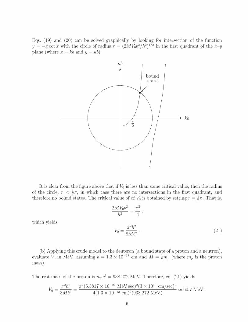
Eqs. (19) and (20) can be solved graphically by looking for intersection of the functiony = −x cot x with the circle of radius r = (2MV0b

2/~2)1/2 in the first quadrant of the x–yplane (where x = kb and y = κb).

kb

κb

π2

boundstate

It is clear from the figure above that if V0 is less than some critical value, then the radiusof the circle, r < 1

2π, in which case there are no intersections in the first quadrant, and

therefore no bound states. The critical value of of V0 is obtained by setting r = 12π. That is,

2MV0b2

~2=π2

4,

which yields

V0 =π2~2

8Mb2. (21)

(b) Applying this crude model to the deuteron (a bound state of a proton and a neutron),evaluate V0 in MeV, assuming b = 1.3 × 10−13 cm and M = 1

2mp (where mp is the proton

mass).

The rest mass of the proton is mpc2 = 938.272 MeV. Therefore, eq. (21) yields

V0 =π2~2

8Mb2=π2(6.5817× 10−22 MeV sec)2(3× 1010 cm/sec)2

4(1.3× 10−13 cm)2(938.272 MeV)≃ 60.7 MeV .

6

(c) Why did I set M = 12mp rather than M = mp in part (b)?

Applying the Schrodinger equation to the bound state of a proton and a neutron, we proceedas in classical mechanics by converting the two-body problem into a one-body problem byseparating off the center-of-mass motion. The corresponding mass employed in the one-body problem is the reduced mass, M = mpmn/(mp + mn). Since mp ≃ mn, it is a goodapproximation to take M = 1

2mp.

REMARK: We have obtained here an estimate of the mean value of the nuclear potentialin light of the fact that the deuteron is a weakly bound system with a bound state energyof Eb ≃ −2.2 MeV. Since Eb ≪ V0 (which was estimated in part (b) to be ∼ 60 MeV), itfollows that our approximation of Eb ≃ 0 [corresponding to the critical value of V0 obtainedin eq. (21)] is justified.

3. Consider a one-dimensional quantum mechanical problem with a time-independent Hamil-tonian, H . The time evolution operator, evaluated in the coordinate basis, also known asthe propagator, is given by,

G(x, t ; x′, 0) = 〈x| e−iHt/~ |x′〉 =∫ ∞

−∞

dp 〈x |p〉 〈p| e−iHt/~ |x′〉 , (22)

where we have taken the initial time to be t0 = 0.

(a) The free particle Hamiltonian is given by H = P 2/(2m). Evaluate the free particlepropagator by explicitly performing the p-integration using eq. (22).

Plugging H = P 2/(2m) into eq. (22), and using the fact that P |p〉 = p |p〉,3

G(x, t ; x′, 0) =

∫ ∞

−∞

dp 〈x |p〉 〈p |x′〉 exp

− ip2t

2m~

.

Using 〈x |p〉 = (2π~)−1/2eipx/~ and 〈p |x′〉 = 〈x |p〉∗, it follows that

G(x, t ; x′, 0) =1

2π~

∫ ∞

−∞

exp

i

~

(

p(x− x′)− p2t

2m

)

dp . (23)

In order to perform the integral given in eq. (23), we “complete the square,” by rewritingthe argument of the exponent in eq. (23) as,

−i[

p2t

2m~− p(x− x′)

~

]

= − it

2m~

[

p− m(x− x′)

t

]2

+im(x − x′)2

2~t.

3Since P is self-adjoint, we also have 〈p|P = 〈p| p (since the eigenvalues of a self-adjoint operator arereal), and 〈p| f(P ) = 〈p| f(p), for any function f(P ) expressed as a Taylor series in P .

7

Plugging this last result back into eq. (23) yields,

G(x, t ; x′, 0) =1

2π~exp

im(x− x′)2

2~t

∫ ∞

−∞

exp

− it

2m~

[

p− m(x− x′)

t

]2

dp .

We now change integration variables by defining p′ ≡ p−m(x−x′)/t. The limits of integrationdo not change and we are left with,

G(x, t ; x′, 0) =1

2π~exp

im(x− x′)2

2~t

∫ ∞

−∞

exp

−itp′ 2

2m~

dp′ .

The integral can now be evaluated by making use of,∫ ∞

−∞

e−iap2 dp = 2

∫ ∞

0

e−iap2 dp = e−iπ/4

√

π

a, for a > 0, (24)

which was derived in the class handout entitled, A Gaussian integral with a purely imaginary

argument. Identifying a ≡ t/(2m~), and noting that a > 0 if we take t > 0 corresponding topropagation forward in time, we end up with,

G(x, t ; x′, 0) = e−iπ/4( m

2π~t

)1/2

exp

im(x− x′)2

2~t

. (25)

Finally, if we interpret e−iπ/4 = i−1/2, we can rewrite eq. (25) as,

G(x, t ; x′, 0) =( m

2πi~t

)1/2

exp

im(x− x′)2

2~t

. (26)

(b) For the one-dimensional harmonic oscillator, where H = P 2/(2m) + 12mω2X2, can

you evaluate the propagator by explicitly performing the p-integration in eq. (22)? Why isthis calculation doomed to failure?

If we try to compute the propagator of the one-dimensional harmonic oscillator using thesame technique as the one employed in part (a), then we would have to evaluate

〈p| exp

−it~

(

P 2

2m+ 1

2mω2X2

)

|x′〉 . (27)

If we could write

exp

−it~

(

P 2

2m+ 1

2mω2X2

)

?= exp

− itP2

2m~

exp

−itmω2X2

2~

, (28)

then it would follow that

〈p| exp

−it~

(

P 2

2m+ 1

2mω2X2

)

|x′〉 ?= exp

−it~

(

p2

2m+ 1

2mω2x′ 2

)

〈p |x′〉 , (29)

after employing the eigenvalue equations for P and X .

8

However, eqs. (28) and (29) are both false. In particular, eq. (28) would be correct if andonly if P 2 and X2 were commuting operators. But, we know that

[

X,P]

= i~I, so that[

X2, P 2]

= X[

X,P 2]

+[

X,P 2]

X

= XP[

X,P]

+X[

X,P]

P + P[

X,P]

X +[

X,P]

PX

= 2i~(XP + PX) . (30)

Thus,[

X2, P 2]

6= 0 (nor is it a c-number). Hence, to evaluate the matrix exponential on theleft hand side of eq. (28), one must employ the Zassenhaus formula for matrix exponentials,4

exp

t(A+B)

= etAetB exp

−12t2[

A,B]

exp

16t3(

2[

B, [A,B]]

+[

A, [A,B]])

· · · ,where the exponents of higher order in t involve nested commutators.

Consequently, the right hand side of eq. (28) must be corrected by multiplying by acomplicated product of exponentials. Hence, it is not possible to simply replace the operatorsP and X with their corresponding eigenvalues in eq. (27).

In fact, one can surmount these difficulties by a clever manipulation of eq. (27). The firststep is to divide up the interval from x to x′ into N equal segments. In the limit of infinitelylarge N , each segment is infinitesimally small. By inserting N complete sets of positioneigenstates and corresponding momentum eigenstates and then formally taking N → ∞,one can develop the so-called path integral representation of the propagator.

The resulting path integral can then be evaluated exactly in the case of the harmonicoscillator. Since we do not have time in this course to pursue this formalism, we shall seekanother technique for computing the propagator of the one-dimensional harmonic oscillator.This is the goal of the next two parts of this problem.

NOTE ADDED:

Perhaps I am being a little too hasty in stating that a direct evaluation of eq. (27)is doomed to failure. Indeed, a direct evaluation has been carried out in F. A. Barone,H. Boschi-Filho and C. Farina, Three methods for calculating the Feynman propagator, Amer-ican Journal of Physics 71, 483 (2003). In this paper, the authors provide three differentmethods of evaluation. The first method corresponds to the method you will employ in parts(c) and (d) of this problem. The third method employs the path integral technique alludedto above. But the second method makes use of the remarkable fact that the exponential ineq. (27) can be expressed as the following product of exponentials,

exp

−it~

(

P 2

2m+ 1

2mω2X2

)

= eiωt/2 exp(−αX2) exp(−βP 2) exp(ωtPX/~) exp(βP 2) exp(αX2) ,

(31)

4The Zassenhaus formula for matrix exponentials is sometimes referred to as the dual of the Baker-Campbell Hausdorff formula. The latter provides a formula for eAeB in terms of a single matrix exponential,whose argument is an infinite series of terms, A+B+ 1

2

[

A,B]

+ · · · , where succeeding terms consist of nestedcommutators. For further details, see, e.g., Fernando Casas, Ander Nurua and Mladen Nadinic, Efficient

computation of the Zassenhaus formula, Comp. Phys. Commun. 183, 2386 (2012).

9

where

α ≡ mω

2~, β ≡ − 1

4m~ω.

Using eq. (31), it is now possible to evaluate eq. (27), with the help of the relation,

〈p′| exp(ωtPX/~ |p〉 = e−iωtδ(p′ − e−iωtp) . (32)

(Can you prove the above result?) As a challenge to the reader, try evaluating eq. (27) usingthe results of eqs. (31) and (32) and then derive the propagator for the harmonic oscillatorusing eq. (22).

(c) Show that G(x, t; x′, 0) = 〈x, t | x′, 0〉, where the |x, t〉 are basis states in the Heisenbergrepresentation. Deduce the following differential equation for G,

i~∂G

∂t= 〈x, t|H |x′, 0〉 ,

where the boundary condition at t = 0 is G(x, 0; x′, 0) = δ(x− x′).

Recall that for basis states in the Heisenberg representation,

|x , t〉 = eiHt/~ |x〉 , (33)

assuming that the Hamiltonian H is time-independent. It immediately follows that |x , t〉satisfies the wrong-sign Schrodinger equation,

i~∂

∂t|x , t〉 = −H |x , t〉 . (34)

For the corresponding bras, we take the adjoint of eqs. (33) and (34) to obtain,

〈x , t| = 〈x| e−iHt/~ , (35)

and

i~∂

∂t〈x , t| = 〈x , t|H , (36)

where we have used the fact that H is self-adjoint.

Eq. (50) then yields,

G(x, t; x′, 0) ≡ 〈x| e−iHt/~ |x′〉 = 〈x , t | x′ , 0〉 ,

after using eqs. (33) and (35). Finally, using eq. (36), it immediately follows that

i~∂G

∂t= 〈x, t|H |x′, 0〉 . (37)

The relevant boundary condition at t = 0 is

G(x, 0; x′, 0) = 〈x , 0 | x′ , 0〉 = 〈x | x′〉 = δ(x− x′) . (38)

10

(d) Evaluate the propagator for the one-dimensional harmonic oscillator by employingthe following steps. First, by using the Heisenberg equations of motion, express P ≡ P (0)in terms of X(t) and X ≡ X(0). Then solve the differential equation obtained in part (c),subject to the boundary condition at t = 0.

The one-dimensional harmonic oscillator Hamiltonian is given by

H =P 2

2m+ 1

2mω2X2 . (39)

To solve for the harmonic oscillator propagator, we shall solve the differential equation givenby eq. (37). Since H is time-independent, H(t) = H(0), and we may employ eq. (39), whereP ≡ P (0) and X ≡ X(0). Our strategy is to rewrite P (0) in terms of the Heisenberg pictureoperators X(t) and X ≡ X(0). To accomplish this, we make use of the Heisenberg equationsof motion,

dP (t)

dt= − i

~

[

P (t) , H(t)]

,dX(t)

dt= − i

~

[

X(t) , H(t)]

.

The commutators are easily evaluated:

[

P (t) , H(t)]

=

[

P (t) ,P 2(t)

2m+ 1

2mω2X(t)

]

= −i~mω2X(t) ,

[

X(t) , H(t)]

=

[

X(t) ,P 2(t)

2m+ 1

2mω2X(t)

]

= i~P (t)

m.

That is, the Heisenberg equations of motion are given by,

dP (t)

dt= −mω2X(t) ,

dX(t)

dt=P (t)

m.

Taking the derivative of dX(t)/dt with respect to time and using the equation for dP (t)/dtyields

d2X(t)

dt= −ω2X(t) .

The solution to this equation is

X(t) =P

mωsinωt+X cosωt , (40)

where P ≡ P (0) and X ≡ X(0).

We can now express P in terms of X(t) and X ,

P =mω

sinωt

[

X(t)−X cosωt]

. (41)

We would like to insert this into eq. (39). In computing P 2, it is important to rememberthat X(t) does not commute in general with X(0). In particular, in light of eq. (40),

[

X , X(t)]

=

[

X ,P

mωsinωt+X cosωt

]

=sinωt

mω

[

X , P ] =i~ sinωt

mω.

11

Thus, squaring eq. (41) yields

P 2 =m2ω2

sin2 ωt

[

X2 +X2 cos2 ωt− cosωt[

X(t)X +XX(t)]

]

=m2ω2

sin2 ωt

[

X2 +X2 cos2 ωt− 2X(t)X cosωt− i~ sinωt cosωt

mω

]

.

Inserting this result into eq. (39), we end up with

H =mω2

2 sin2 ωt

[

X2(t) +X2 cos2 ωt− 2X(t)X cosωt− i~ sinωt cosωt

mω

]

+ 12mω2X2 . (42)

We can now evaluate 〈x , t|H |x′ , 0〉 by employing the eigenvalue equations,

X(t) |x , t〉 = x |x , t〉 , X |x , 0〉 = X(0) |x , 0〉 = x |x , 0〉 .

It then follows that

〈x , t|H |x′ , 0〉 =

mω2

2 sin2 ωt

[

x2 + x′ 2 cos2 ωt− 2xx′ cosωt− i~ sinωt cosωt

mω

]

+ 12mω2x′ 2

〈x , t | x , 0〉

=

mω2

2 sin2 ωt

[

x2 + x′ 2 − 2xx′ cosωt]

− i~ω cosωt

2 sinωt

〈x , t | x , 0〉

Plugging this result into eq. (37) yields the following differential equation,

∂G

∂t=

−imω2

2~ sin2 ωt

[

x2 + x′ 2 − 2xx′ cosωt]

− ω cosωt

2 sinωt

G , (43)

subject to the boundary condition specified by eq. (38).

Obtaining the solution to eq. (43) is straightforward. Integrating over t, and making useof∫

dt

sin2 ωtdt = − 1

ωcotωt ,

∫

cosωt

sin2 ωtdt = − 1

ω sinωt,

∫

cosωt

sinωtdt =

1

ωln | sinωt| ,

we end up with

G(x, t ; x′, 0) = g(x, x′) exp

imω[

(x2 + x′ 2) cosωt− 2xx′]

2~ sinωt− 1

2ln | sinωt|

,

where g(x, x′) is a function of x and x′ to be determined. We can rewrite G(x, t ; x′, 0) inthe following form,

G(x, t ; x′, 0) = g(x, x′)| sinωt|−1/2 exp

imω[

(x2 + x′ 2) cosωt− 2xx′]

2~ sinωt

. (44)

12

We now impose the boundary condition specified by eq. (38). However, we cannot justset t = 0 in eq. (44), since the resulting expression is not well defined. Instead, we shallconsider the limit as t→ 0+ and impose the condition that5

limt→0+

G(x, t ; x′, 0) = δ(x− x′) .

Since cosωt ≃ 1 and sinωt ≃ ωt as t→ 0, it follows that

δ(x− x′) = limt→0+

g(x, x′)(ωt)−1/2 exp

im(x− x′)2

2~t

. (45)

Eq. (45) should be compared with the following representation of the delta function6

δ(x− x′) = lim∆→0

1

(π∆2)1/2exp

−(x− x′)2

∆2

, (46)

If we define ∆2 ≡ 2i~t/m, then we can therefore identify7

g(x, x′) =( mω

2πi~

)1/2

. (47)

Plugging this result back into eq. (44), we end up with,

G(x, t ; x′, 0) =( mω

2πi~ sinωt

)−1/2

exp

imω[

(x2 + x′ 2) cosωt− 2xx′]

2~ sinωt

, (48)

assuming that 0 < t < π/ω, in which case we can drop the absolute value signs from thefactor | sinωt| that appears in the prefactor of the exponential in eq. (44).8

(e) Check that in the limit of ω → 0, the result of part (d) reduces to the free particlepropagator obtained in part (a).

If one evaluates eq. (48) in the limit of ω → 0, the end result is,

G0(x, t ; x′, 0) =

( m

2πi~t

)1/2

exp

im(x − x′)2

2~t

, (49)

which is the expression for the free-particle propagator previously obtained in eq. (26).5The t→ 0 limit should be taken such that t = 0 is approached from the positive side (this is the meaning

of the symbol t→ 0+), since one is typically interested in propagation forward in time, i.e. t > 0.6See e.g., eq. (1.10.19) of Ramamurti Shankar, Principles of Quantum Mechanics, 2nd edition, p. 61.7Strictly speaking, these steps are valid only for Re∆2 > 0. When ambiguities of this nature arise in

quantum mechanics, the safest procedure is to add an infinitesimal real part to ∆2 in such a way thatconvergence is assured. At the end of the calculation, this infinitesimal quantity can be taken to zero.

8The result given in eq. (48) is ambiguous, since it is not clear how to interpret i−1/2 in the prefactor.One can show that the naive choice, i−1/2 = e−iπ/4, is correct only for 0 < t < π/ω. This ambiguity isassociated with the fact that sinωt = 0 at t = π/ω which means that the propagator diverges at this point(called the first caustic). For values of t > π/ω, an additional phase factor arises that cannot be fixed by thelimiting procedure of eqs. (45)–(47). A simple way of deriving this phase factor is given in Nora S. Thornberand Edwin F. Taylor, American Journal of Physics, 66, 1022 (1998). You can also find references there tothe original literature and references to the few textbooks that address this phase ambiguity.

13

4. The partition function is defined by,

Z(β) ≡ Tr e−βH ,

where H is a time-independent Hamiltonian operator and β is a real positive parameter.

(a) In the case of a one-dimensional quantum mechanical problem, show that

Z(β) =

∫

G(x,−i~β ; x, 0) dx ,

where the propagator is defined by,

G(x, t; x′, 0) ≡ 〈x| e−iHt/~ |x′〉 . (50)

Evaluating the trace in a coordinate basis,

Z(β) ≡ Tr e−βH =

∫

d3x 〈~x| e−βH |~x〉 =∫

d3xG(~x, t;~x, 0)

∣

∣

∣

∣

t=−i~β

,

which yields the result quoted in eq. (50).

(b) Show that the ground state energy E0 is given by:

E0 = limβ→∞

− 1

Z

∂Z

∂β.

One can also compute Z(β) by evaluating the trace with respect to a basis of energy eigen-states. Assuming that the basis states are normalized to unity, 〈Em|En〉 = δmn, whereH |En〉 = En |En〉, it follows that

Z(β) ≡ Tr e−βH =∑

n

〈En| e−βH |En〉 =∑

n

e−βEn 〈En|En〉 =∑

n

e−βEn , (51)

where I have adopted a convention in which Em ≤ En form < n. Henceforth, we will assumethat the ground state energy E0 is non-degenerate. Hence, eq. (51) yields

− 1

Z

∂Z

∂β=

∑

n

En e−βEn

∑

n

e−βEn

=E0 e

βE0 + E1 eβE1 + E2 e

βE2 + · · ·eβE0 + eβE1 + eβE2 + · · ·

=E0 + E1 e

β(E1−E0) + E2 eβ(E2−E0) + · · ·

1 + eβ(E1−E0) + eβ(E2−E0) + · · · ,

14

where E0 is the (non-degenerate) ground state energy as previously noted. This means thatEn − E0 > 0 for n = 1, 2, 3, . . .. Taking the limit as β → ∞, it follows that e−β(En−E0) → 0for all n = 1, 2, 3, . . .. Consequently,

E0 = limβ→∞

− 1

Z

∂Z

∂β. (52)

REMARK: Using eq. (51), one can immediately establish the following result,∫ ∞

0

e−βEZ(β)dβ =∑

n

1

E + En.

However, in the case of the harmonic oscillator, both sides of this relation are divergent.Thus, this relation does not provide a method for computing the energy levels of the harmonicoscillator. Nevertheless, all is not lost as we now examine in parts (c) and (d) of this problem.

(c) Using the results of part (b) of this problem and part (d) of Problem 3, compute theground state energy of the one-dimensional harmonic oscillator.

One can now evaluate Z(β) as follows. First, we set x′ = x and t = −i~β in the expressionfor G(x, t ; x′, 0) given in eq. (48). Using sin(iz) = i sinh z and cos(iz) = cosh z, we obtain,9

G(x,−i~β ; x, 0) =(

mω

2π~ sinh β~ω

)−1/2

exp

− mωx2(cosh β~ω − 1)

~ sinh β~ω

. (53)

It follows that

Z(β) =

∫ ∞

−∞

dxG(x,−i~β ; x, 0) = 1

2

(

2

cosh β~ω − 1

)1/2

.

In light of the identity, sinh2(z/2) = 12(cosh z − 1), we can rewrite Z(β) as

Z(β) =1

2 sinh(

12β~ω

) , (54)

which yields,

− 1

Z

∂Z

∂β= 1

2~ω coth

(

12β~ω

)

.

Finally, we use eq. (52) to compute the ground state energy.

E0 = limβ→∞

− 1

Z

∂Z

∂β= 1

2~ω ,

as expected for the ground state energy of the harmonic oscillator.9In contrast to eq. (48), no phase ambiguities arise in the derivation of eq. (53). Indeed, since β > 0, the

prefactor is equal to the positive inverse square root of a positive quantity.

15

(d) Consider the the propagator for a one-dimensional quantum system governed bya time-independent Hamiltonian with only discrete (bound state) energy levels, En, forn = 0, 1, 2, 3, . . .. Using eq. (50), show that the full energy spectrum of H can be determinedfrom10

Tr e−iHt/~ =

∫ ∞

−∞

dxG(x, t ; x, 0) =∑

n

〈En| e−iHt/~ |En〉 =∞∑

n=0

e−iEnt/~ . (55)

Strictly speaking, the sums on the right-hand side of eq. (57) are not convergent. However,one can give mathematical meaning to these sums by extending the time parameter to thecomplex plane.

In particular, let t = −i~β (where β is a positive real parameter). Using eq. (57), obtainall the energy eigenvalues of the one-dimensional harmonic oscillator.

In analogy with part (a) of this problem, we can write Tr e−iHt/~ in two different ways. Withrespect to the coordinate basis,

Tr e−iHt/~ =

∫ ∞

−∞

dx 〈x| e−iHt/~ |x〉 =∫ ∞

−∞

G(x, t ; x, 0) .

where we have made use of eq. (50). Alternatively, we can compute the trace with respectto the energy eigenstate basis,

Tr e−iHt/~ =∑

n

〈En| e−iHt/~ |En〉 =∑

n

e−iEnt/~ ,

under the assumption that the energy eigenstates are normalized to unity. Hence, eq. (55)is established. If we now put t = −i~β, then we obtain

Z(β) ≡ Tr e−βH =∑

n

e−βEn , (56)

which is a result that was previously obtained in part (b) [cf. eq. (51)].

In part (c) we derived an explicit formula for Z(β) [cf. eq. (54)]. We can rewrite thisresult in the following way:

Z(β) =1

2 sinh(

12β~ω

) =1

eβ~ω/2 − e−β~ω/2=

e−β~ω/2

1− e−β~ω= e−β~ω/2

∞∑

n=0

e−βn~ω =

∞∑

n=0

e−β(n+ 1

2)~ω .

Comparing with eq. (56), we conclude that the energy levels of the harmonic oscillator are

En = ~ω(n+ 12) .

10In eq. (57), the trace is expressed as a diagonal sum of matrix elements by employing two different basischoices (the coordinate basis and the energy basis, respectively). Of course, the trace is a basis-independentquantity, so one may choose any orthonormal basis to compute it.

16

5. Consider a particle in one dimension trapped between two impenetrable walls at x = 0and x = L.

(a) Determine the bound state energy levels, En, of the particle. (Here, n labels thepossible energy eigenvalues: n = 1 is the ground state, n = 2 is the first excited state, etc.).

We solve the time-independent Schrodinger equation,

Hψ(x) = − ~2

2m

d2ψ(x)

dx2= Eψ(x) , (57)

subject to the boundary conditions, ψ(0) = ψ(L) = 0, which are a consequence of the twoimpenetrable walls at x = 0 and x = L. As usual, we define

k =

√

2mE

~2,

where k > 0. Then, the solution to eq. (57) is

ψ(x) =

A sin kx , for 0 ≤ x ≤ L,

0 , for x > L and x < −L,

after imposing the boundary condition ψ(0) = 0. We next impose the boundary conditionψ(L) = 0, which yields,

kL = nπ , for any positive integer n. (58)

Note that since k > 0, n cannot be negative, and n = 0 is not allowed since this wouldcorrespond to ψ(x) = 0, which is not an eigenfunction of H . Eq. (58) then yields,

En =~2k2

2m=π2~2n2

2mL2. (59)

The normalization constant A is easily determined by setting

1

|A|2 =

∫ L

0

sin2(nπx

L

)

dx = 12L ,

which yields A =√

2/L after setting the arbitrary phase factor to unity. It is convenient towrite the expressions for the energy eigenstates with the help of the Heavyside step function.Then, the eigenfunction corresponding the the nth energy level is given by

ψn(x) =

√

2

Lsin

(nπx

L

)

[Θ(x)−Θ(x− L)] , (60)

where Θ(x) is the Heavyside step function, and the quantity Θ(x) − Θ(x − L) in eq. (60)ensures that the wave function is zero beyond the two impenetrable walls at x = 0 andx = L.

17

(b) Suppose that at time t = 0, the state of the particle is given by the wave function

ψ(x, t = 0) = Ax(L− x) [Θ(x)−Θ(x− L)] ,

where Θ(x) is the Heavyside step function and A is a normalization constant.

If an energy measurement is performed at time t = 0, what is the probability thatthe particle will be observed to be in the ground state? Find an exact expression for theprobability that the particle will be observed to be in a state of energy En (for any positiveinteger n).

The normalization constant is determined in the usual way,

1

|A|2 =

∫ L

0

x2(L− x)2dx = L2(

13− 1

2+ 1

5

)

=L5

30.

Hence, after setting the the arbitrary phase factor to unity,

A =

√

30

L2.

Thus,

ψ(x, t = 0) =

√

30

L2x(L− x) [Θ(x)−Θ(x− L)] , (61)

Next, we expand ψ(x, t = 0) in terms of energy eigenstates,

ψ(x, 0) =

∞∑

n=1

cnψn(x) , (62)

where the energy eigenstates (which are a complete set of states), are given by eq. (60).Using the fact that the ψn(x) are orthonormal,

∫ L

0

ψ∗n(x)ψm(x) dx = δnm ,

we can multiply eq. (62) on the left by ψ∗n(x) and integrate to project out the coefficients cn.

Thus,

cn =

∫ L

0

ψ∗n(x)ψ(x, 0) dx =

(

30

L5

)1/2(2

L

)1/2 ∫ L

0

x(L− x) sin(πnx

L

)

dx .

after the change of variables, y = πx/L,

cn =2√15

π2

∫ π

0

y(

1− y

π

)

sin(ny)dy .

18

Employing the integrals,∫ π

0

y sin(ny)dy = − π

n(−1)n ,

∫ π

0

y2 sin(ny)dy = − π2

n(−1)n +

2

n3

[

(−1)n − 1]

,

we end up with

cn =4√15

π3n3

[

1− (−1)n]

.

We conclude that the probability of finding the particle in the state with energy En, denotedby Pn, is given by

Pn = |cn|2 =240

π6n6

[

1− (−1)n]2 .

The ground state corresponds to n = 1. Thus, the probability that the particle will beobserved to be in the ground state is

P1 =960

π6= 0.9986 .

This means that ψ(x, 0) is a pretty good approximation to the ground state energy eigen-function!

(c) Evaluate the expectation value of the Hamiltonian with respect to the wave functiongiven in eq. (61). What is the average value of the energy at time t = 0?

The average energy is given by the expectation value of the Hamiltonian. Thus, in light ofeq. (57),

〈E〉 = 〈ψ|H |ψ〉 = − ~2

2m

∫ L

0

ψ∗(x)d2ψ(x)

dx2dx .

Plugging in eq. (61),

〈E〉 = 30

L5

∫ L

0

x(L− x)

(

− ~2

2m

d2

dx2

)

x(L− x)dx =30~2

mL5

∫ L

0

x(L− x)dx =5~2

mL2. (63)

WARNING :

The calculation presented above is too naive, although the end result turns out to becorrect. Note that starting from eq. (61), it follows that

dψ

dx=

√

30

L2

(L− 2x) [Θ(x)−Θ(x− L)] + x(L− x) [δ(x)− δ(x− L)]

, (64)

19

after using δ(x) = dΘ(x)/dx. Luckily, the second term on the right hand side of eq. (64)does not contribute, since xδ(x) = 0 and (L− x)δ(x− L) = 0. Hence,

dψ

dx=

√

30

L2

(L− 2x) [Θ(x)−Θ(x− L)]

.

However, when we take the second derivative,

d2ψ

dx2=

√

30

L2

−2 [Θ(x)−Θ(x− L)] + (L− 2x) [δ(x)− δ(x− L)]

,

we cannot immediately discard the terms proportional to the delta functions. Indeed, (L−2x)δ(x) = Lδ(x) and (L− 2x)δ(x− L) = −Lδ(x − L), Hence,

d2ψ

dx2=

√

30

L2

−2 [Θ(x)−Θ(x− L)] + L [δ(x) + δ(x− L)]

,

When we compute 〈E〉 more carefully, we obtain

〈E〉 = − ~2

2m

∫ L

0

ψ∗(x)d2ψ(x)

dx2dx

= −15~2

mL5

∫ ∞

−∞

x(L− x) [Θ(x)−Θ(x− L)]

−2 [Θ(x)−Θ(x− L)] + L [δ(x) + δ(x− L)]

.

Since an overall factor of x(L − x) appears in the integrand, we can use it to kill the deltafunction terms, i.e., x(L− x) [δ(x) + δ(x− L)] = 0. It then follows that

〈E〉 = 30~2

mL5

∫ L

0

x(L− x)dx =5~2

mL2.

The reason I mention all this is that keeping track of the terms that arise by takingmultiple derivatives of the Heavyside step function will sometimes matter. In particular,if you were to calculate 〈E2〉 = 〈ψ|H2 |ψ〉, the naive calculation of the integrand wouldgive zero, but the correct calculation would yield terms proportional to the derivative of thedelta function, which contributes to the final result. Indeed, the correct calculation yields〈E2〉 = 30~4/(m2L4). (Try it!)

(d) The expectation value of H can be computed by a different method than the oneused in part (c). First, expand ψ(x, 0) as a linear combination of energy eigenstates, andthen show that the expectation value of H can be expressed as an infinite sum. Using thistechnique, obtain an expression for the average value of the energy at time t = 0, and thenemploy the result obtained in part (c) to determine the value of the sum,

∞∑

n=0

1

(2n+ 1)4.

20

We can also compute 〈E〉 by inserting a complete set of energy eigenstates,

〈E〉 = 〈ψ|H |ψ〉 =∑

n

〈ψ|H |En〉 〈En|ψ〉 =∑

n

En 〈ψ|En〉 〈En|ψ〉 =∞∑

n=1

En|cn|2 , (65)

after making use of eq. (62) and identifying cn = 〈En|ψ〉.In part (b), we computed

|cn|2 =240

π6n6

[

1− (−1)n]2 =

960

π6n6, for n odd,

0 , for n even.

Inserting this result into eq. (65) and making use of eq. (59), we end up with

〈E〉 = 480~2

π4mL2

∑

n>0n odd

1

n4,

which we can rewrite as

〈E〉 = 480~2

π4mL2

∞∑

n=0

1

(2n+ 1)4. (66)

Comparing eqs. (63) and (66), we conclude that

∞∑

n=0

1

(2n+ 1)4=π4

96. (67)

ADDED NOTE:

Sums such as the one given in eq. (67) are related to the famous Riemann zeta function,11

ζ(z) =∞∑

n=1

1

nz=

1

1− 21−z

∞∑

n=1

(−1)n+1 1

nz,

where the first sum is valid for Re z > 1 and the second sum is valid for Re z > 0 (assumingthat z 6= 1 where the Riemann zeta function diverges). It then follows that

∑

n>0n odd

1

nz=

1

2

∞∑

n=1

1

nz+

1

2

∞∑

n=1

(−1)n+1 1

nz= (1− 2−z)ζ(z) , for Re z > 1.

11See e.g., I.S. Gradshteyn and I.M. Ryzhik, Table of Integral, Series and Products, 8th edition (AcademicPress, Waltham, MA, 2015) pp. 1046–1049.

21

It is well known that ζ(4) = π2/90. Hence,

∑

n>0n odd

1

n4=π4

96.

in agreement with eq. (67).

(e) After preparing the state given by eq. (61) at time t = 0, suppose that instead ofperforming an energy measurement at time t = 0, I wait a while and then make the firstenergy measurement at a later time t > 0. Do any of the results obtained in parts (b) and (c)change? Explain.

The results of parts (b) and (c) do not change as a function of time. To prove this, we firstnote that eq. (60) is equivalent to

|ψ(0)〉 =∑

n

cn |E〉 ,

when evaluated with respect to the coordinate basis. Multiplying on the left by 〈Em| andusing 〈Em|En〉 = δmn, it immediately follows that cn = 〈En|ψ(0)〉. Next, we recall that

|ψ(t)〉 = U(t) |ψ(0)〉 = U(t)∑

n

|En〉 〈En|ψ(0)〉 =∑

n

cne−iEnt/~ |En〉 (68)

where we have used the fact that the time evolution is given by U(t) = exp(

−iHt/~)

for atime-independent Hamiltonian, and H |En〉 = En |En〉. It immediately follows that

ψ(x, t) =∞∑

n=1

cne−iEnt/~ψn(x) , (69)

after evaluating eq. (68) with respect to the coordinate basis. From eq. (69), we conclude thatthe probability of a state with wave function ψ(x, t) to be observed in an energy eigenstatewith energy En at time t is given by

|cne−iEnt/~|2 = |cn|2 ,

which is indeed time-independent.

To see that 〈E〉 is also time-independent, we make use of Ehrenfest’s equation,

d

dt〈Ω〉 = i

~

⟨

[H , Ω]⟩

+

⟨

∂Ω

∂t

⟩

.

Setting ω = H , it follows thatd

dt〈E〉 = 0 ,

for any time-independent Hamiltonian. This is the quantum mechanical statement of energyconservation.

22

6. Consider a periodic potential in one-dimension which satisfies V (x+ ℓ) = V (x).

(a) Show that the translation operator T = exp(−iℓP/~) commutes with the Hamilto-nian:

H =P 2

2m+ V (x) . (70)

We first note that [P 2 , T ] = 0, since P commutes with any function of P . Thus, we focuson [T , V (X)]. Consider the action of this commutator on an arbitrary basis state |x〉,

[T , V (X)] |x〉 =

TV (X)− V (X)T

|x〉 =(

V (x)− V (X))

T |x〉 , (71)

where we have used V (X) |x〉 = V (x) |x〉, where X |x〉 = x |x〉. Using the result of problem5(c) on Problem Set 1 (with P = ~K), it follows that

T |x〉 = exp(−iℓP/~) |x〉 = |x+ ℓ〉 . (72)

Since V (X) |x+ ℓ〉 = V (x+ ℓ) |x+ ℓ〉, it then follows from eqs. (71) and (72) that

[T , V (X)] |x〉 =(

V (x)− V (x+ ℓ))

|x+ ℓ〉 = 0 , (73)

where we have used the periodicity of V (x) in the final step above. Since eq. (73) is true foran arbitrary basis state |x〉, it follows that [T , V (X)] = 0.

(b) We may choose the energy eigenstates to be simultaneous eigenstates of the transla-tion operator T . Show that the general form of such eigenfunctions is:

ψ(x) = exp(ipx/~)up(x) .

where up(x+ℓ) = up(x). That is, the eigenfunctions are plane waves modulated by a functionwith the periodicity of the potential.

Consider the eigenvalue problem for T ,

T |ψ〉 = t |ψ〉 . (74)

To determine the possible values of t, examine eq. (74) in the p-representation. Since

〈p|T |ψ〉 = 〈p| exp(−iℓP/~) |ψ〉 = e−iℓp/~ 〈p|ψ〉 ,

we can conclude thatt = e−iℓp/~ . (75)

Next, we consider the eigenvalue equation for T in the x-representation. Using eqs. (74)and (75),

〈x| T |ψ〉 = e−iℓp/~ 〈x|ψ〉 . (76)

23

In light of eq. (72), T |x〉 = |x+ ℓ〉. It follows that 〈x| T = 〈x− ℓ|. To verify this lastassertion,12 consider

〈x| T |x′〉 = 〈x|x′ + ℓ〉 = δ(x− x′ − ℓ) ,

when we act with T to the right. If we act with T to the left we will get the same result if〈x|T = 〈x− ℓ|, namely,

〈x| T |x′〉 = 〈x− ℓ|x′〉 = δ(x− x′ − ℓ) ,

Consequently, eq. (76) yields

〈x− ℓ|ψ〉 = e−iℓp/~ 〈x|ψ〉 .

which we can rewrite asψ(x− ℓ) = e−iℓp/~ψ(x) . (77)

Although ψ(x) is not a periodic function, it is straightforward to check that e−ipx/~ψ(x)is periodic, since the equation,

e−i(x−ℓ)p/~ψ(x− ℓ) = e−ipx/~ψ(x) ,

is equivalent to eq. (77). Thus, we introduce the notation,

up(x) ≡ e−ipx/~ψ(x) .

Then,ψ(x) = eipx/~up(x) ,

where up(x+ ℓ) = up(x). This result is known as Bloch’s Theorem. The description of ψ(x)as a plane wave modulated by a function that possesses the periodicity of the potential V (x)is called a Bloch wave.

12Another way to derive 〈x|T = 〈x− ℓ| is as follows. The action of the operator T on the ket |x〉is T |x〉 ≡ |Tx〉. Likewise, the action of the operator T on the bra 〈x| is 〈x|T ≡

⟨

T †x∣

∣. Since P is

hermitian, it follows that T † = exp(iℓP/~). Thus∣

∣T †x⟩

= T † |x〉 = |x− ℓ〉 and the adjoint of∣

∣T †x⟩

is⟨

T †x∣

∣ = 〈x|T = 〈x− ℓ|.

24

APPENDIX: An alternative solution to Problem 6

Since V (x+ ℓ) = V (x), we can expand V (X) in a Fourier series,

V (X) =∞∑

n=−∞

cn exp(2πinX/ℓ) .

To compute TV (X), where T = exp(−iℓP/~), we need to calculate the product of twoexponentials. Here we make use of the identities,

eAeB = exp(

A+B + 12[A,B]

)

, (78)

eBeA = exp(

A+B − 12[A,B]

)

,

under the assumption that[

A, [A,B]]

=[

B, [A,B]]

= 0. Using [X , P ] = i~I,

TV (X) =∑

n

cn exp

[

−iℓP~

+2πinX

ℓ− iπn

]

=∑

n

cn exp

[

−iℓP~

+2πin(X − ℓ)

ℓ+ iπn

]

= V (X − ℓ)T = V (X)T .

Hence, we have demonstrated that [T , V (X)] = 0.

It then follows that [H , T ] = 0. Thus, we can choose |ψ〉 = |E, t〉 to be a simultaneouseigenstate of H and T . That is, H |E, t〉 = E |E, t〉 and T |E, t〉 = t |E, t〉. Consequently,

〈x|HT |E, t〉 = tE 〈x|E, t〉 , 〈x|TH |E, t〉 = E 〈x− ℓ|E, t〉 ,after noting [cf. footnote 12] that 〈x|T = 〈x− ℓ|. Since HT = TH , it follows that

ψ(x− ℓ) = tψ(x) , (79)

where ψ(x) ≡ 〈x|E, t〉. Finally, we compute t by evaluating 〈p|T |E, t〉 in two different ways,

〈p|T |E, t〉 = t 〈p|E, t〉 ,and

〈p|T |E, t〉 = 〈p| exp(−iℓP/~) |E, t〉 = exp(−iℓp/~) 〈p|E, t〉 .Subtracting the last two equations yields t = e−iℓp/~. Plugging this back into eq. (79) yields

ψ(x− ℓ) = e−iℓp/~ψ(x) , (80)

which reproduces eq. (77). The final step is the same as in our previous solution. Namely,we introduce,

up(x) ≡ e−ipx/~ψ(x) .

and show that eq. (80) implies that up(x− ℓ) = up(x). Hence, we conclude as before that

ψ(x) = eipx/~up(x) ,

where up(x+ ℓ) = up(x).

25