Phylogenetic Analysis

Han Liang, Ph.D. Assistant Professor of Bioinformatics and Computational Biology

UT MD Anderson Cancer Center

Outline

•  Basic Concepts •  Tree Construction Methods Distance-based methods Character-based methods

•  Bootstrap Analysis

What is Phylogenetics

•  The term phylogenetics derives from Greek –  phyle (φυλή) :“tribe” and “race”; –  genetikos (γενετικός): “relative to birth”

•  "Phylogenetics" is the study or estimation of the evolutionary history that underlies that biological diversity.

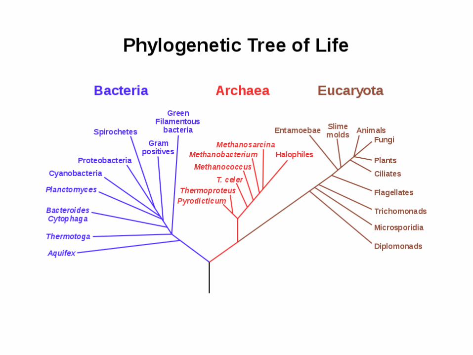
•  This organization is visually described through "trees".

Molecular phylogenetics

Molecular phylogenetics: the study of evolutionary relationships among organisms or genes by using molecular data (e.g., DNA or protein sequences) and statistical techniques.

Molecular systematics, if the relationships of organisms are the concern.

Why Study Molecular Phylogenetics?

•  Provides insights into relationships among

organisms - through "species" trees. •  Provides insights into the evolution and

history of genes - through "gene" trees.

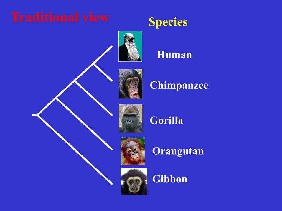
Example: Phylogeny of human and apes

•  Apes – Great apes:

• chimpanzee, bonobo (pygmy chimp), gorilla, orangutan

– Lesser apes: • Gibbon

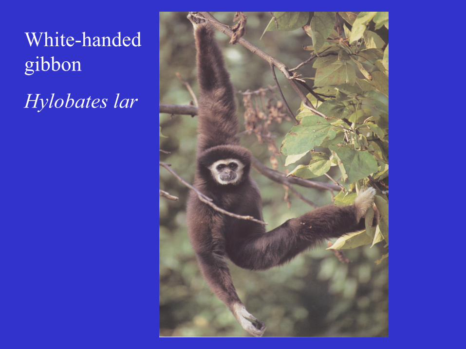
White-handed gibbon

Hylobates lar

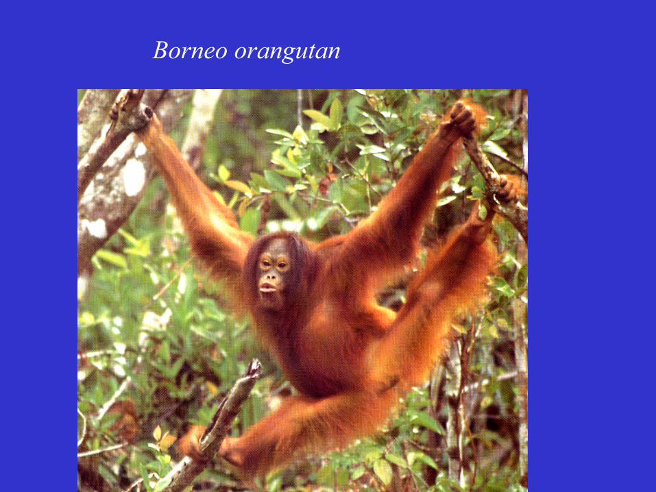
Borneo orangutan

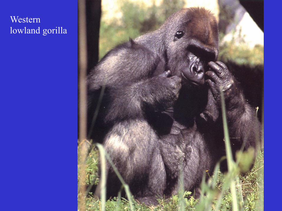
Western lowland gorilla

Common chimpanzee

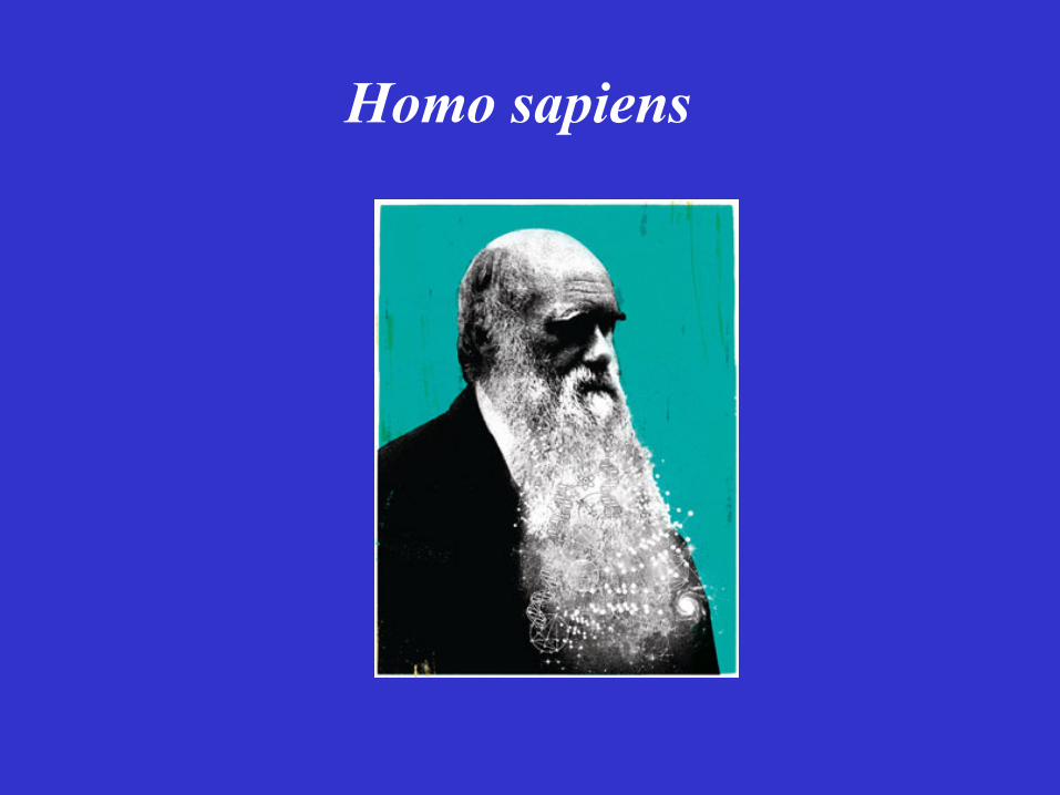
Homo sapiens

Human

Chimpanzee

Gorilla

Orangutan

Gibbon

Species Traditional view

Human

Chimpanzee

Gorilla

Orangutan

Gibbon

Human

Chimpanzee

Gorilla

Orangutan

Gibbon

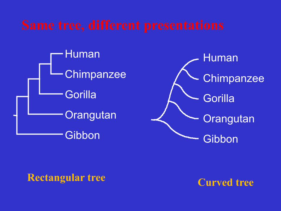
Curved tree Rectangular tree

Same tree, different presentations

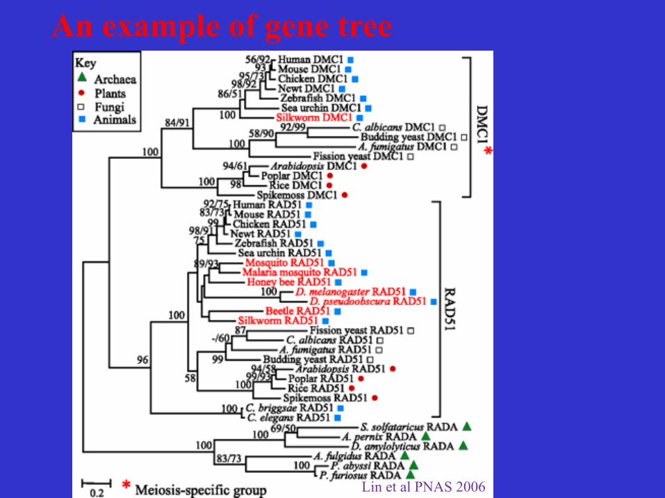
An example of gene tree

Lin et al PNAS 2006

Objectives

•  To understand the basic concepts and terminology of molecular phylogenetics;

•  To understand tree topologies and how to read them

•  To understand the basic concepts of different tree building methods

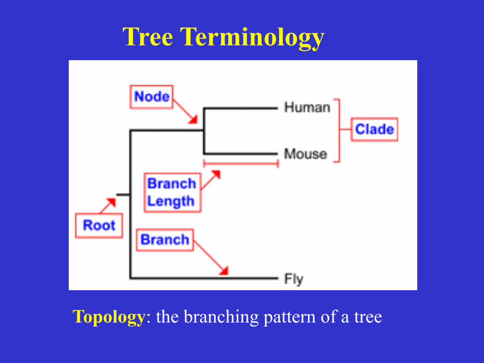
Tree Terminology

Topology: the branching pattern of a tree

A

B

C

D

E

F

G H

I

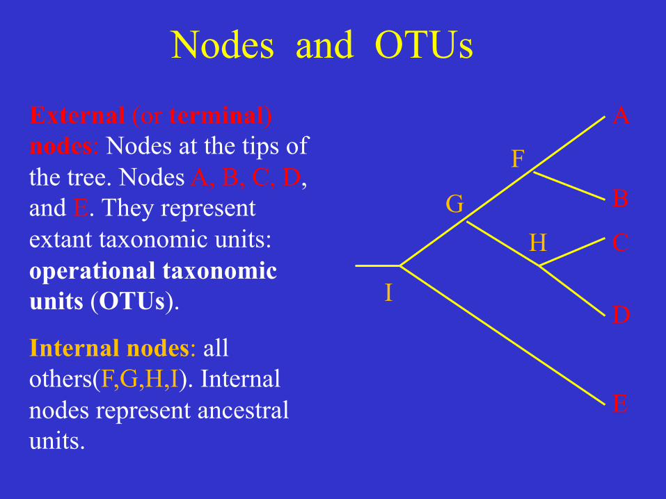
Nodes and OTUs External (or terminal) nodes: Nodes at the tips of the tree. Nodes A, B, C, D, and E. They represent extant taxonomic units: operational taxonomic units (OTUs).

Internal nodes: all others(F,G,H,I). Internal nodes represent ancestral units.

Time

R

A

B

C

D

E

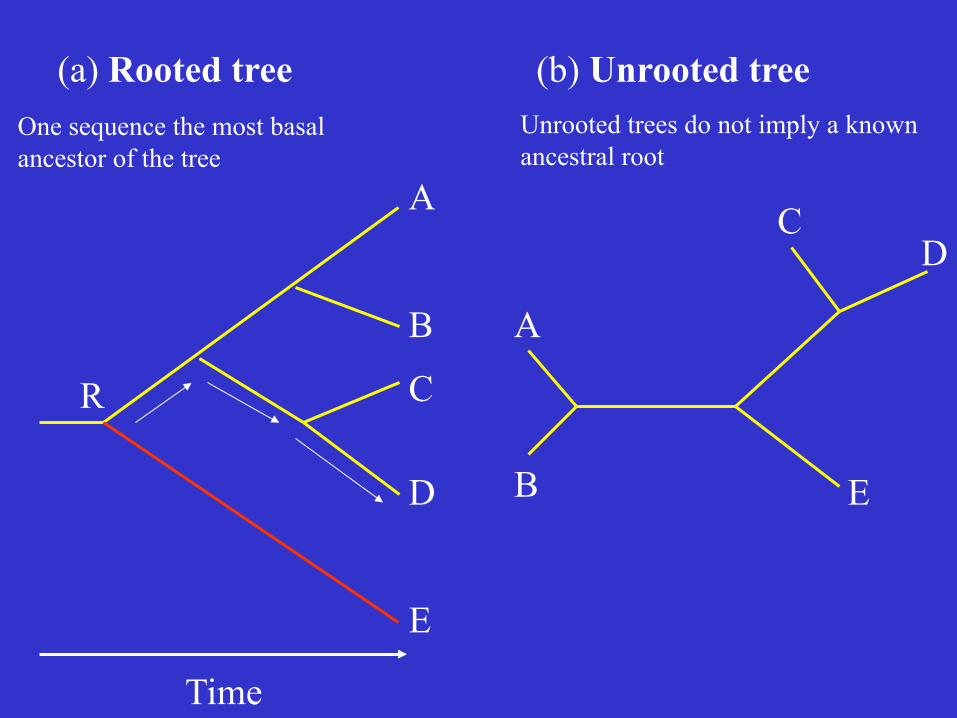
(a) Rooted tree (b) Unrooted tree

A

B

C D

E

One sequence the most basal ancestor of the tree

Unrooted trees do not imply a known ancestral root

A

B C

D

E

F G

H

I 2

6

3 2

1

1 1

2 (a) Unscaled

E

A

B C

D 6

2 1

2

3 2

1

1 unit

(b) Scaled

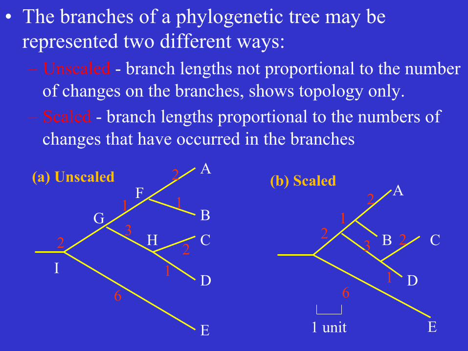
•  The branches of a phylogenetic tree may be represented two different ways: – Unscaled - branch lengths not proportional to the number

of changes on the branches, shows topology only. – Scaled - branch lengths proportional to the numbers of

changes that have occurred in the branches

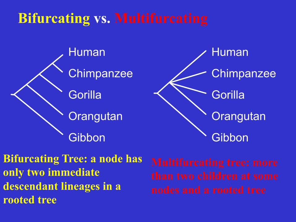
Bifurcating vs. Multifurcating

Bifurcating Tree: a node has only two immediate descendant lineages in a rooted tree

Multifurcating tree: more than two children at some nodes and a rooted tree

Human

Chimpanzee

Gorilla

Orangutan

Gibbon

Human

Chimpanzee

Gorilla

Orangutan

Gibbon

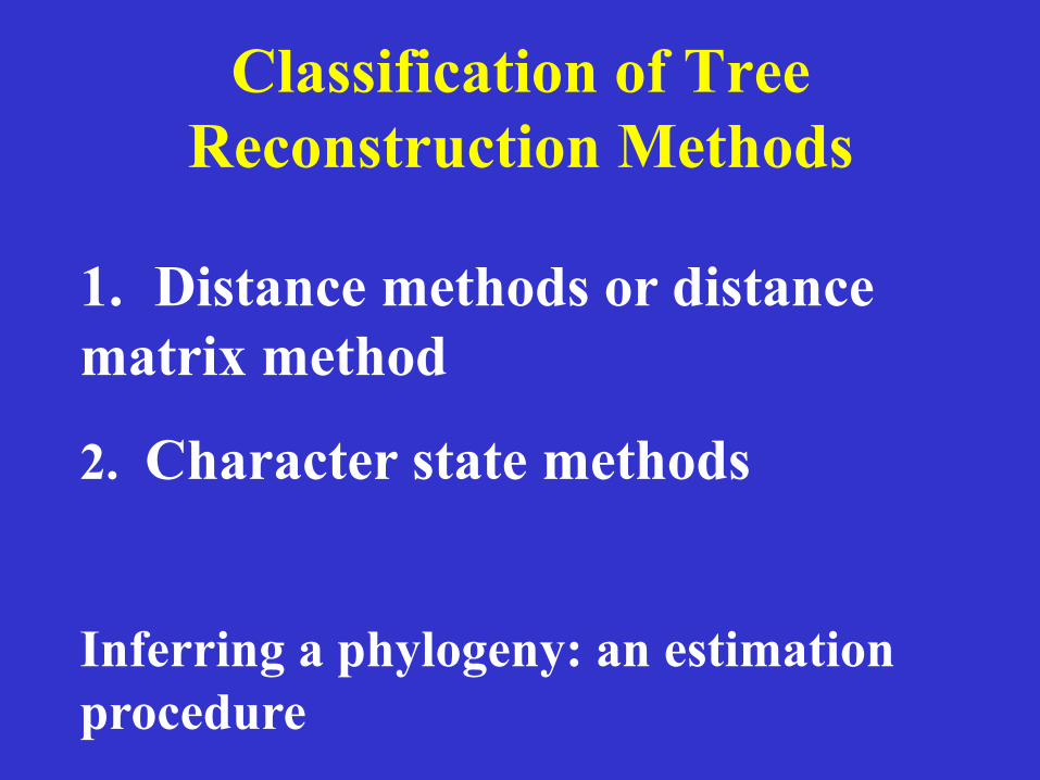
Classification of Tree Reconstruction Methods

1. Distance methods or distance matrix method

2. Character state methods

Inferring a phylogeny: an estimation procedure

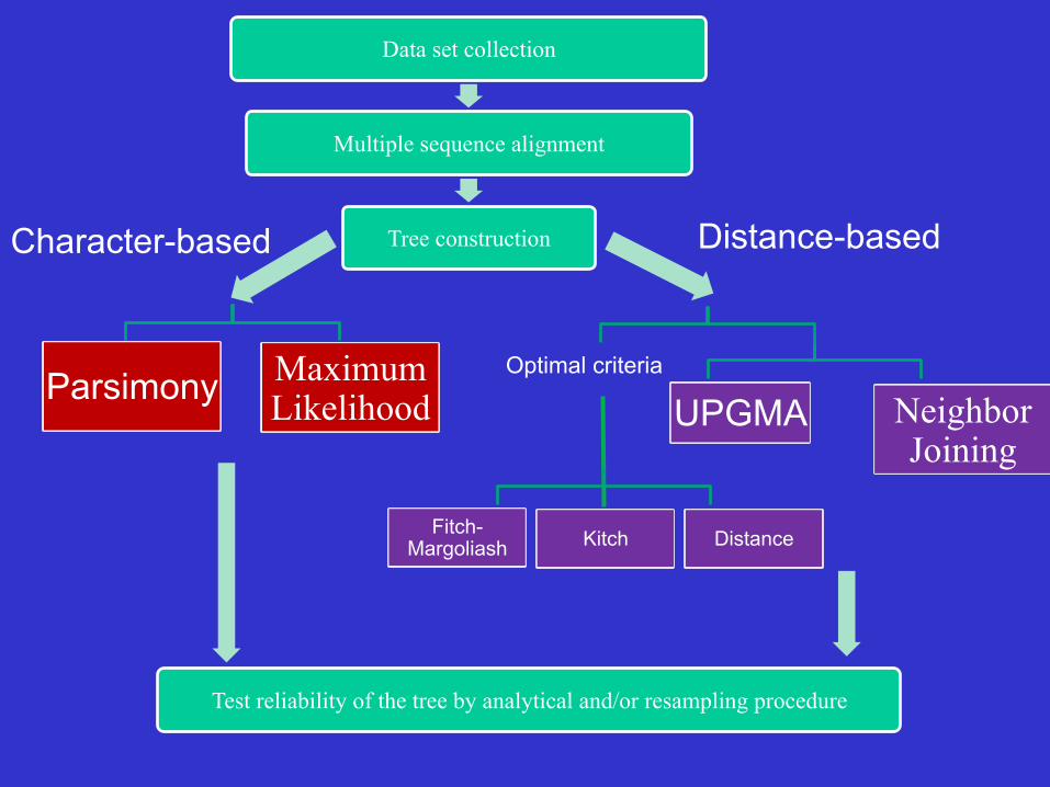
Data set collection

Multiple sequence alignment

Tree construction Character-based Distance-based

Parsimony Maximum Likelihood UPGMA Neighbor

Joining

Optimal criteria

Fitch-Margoliash Kitch Distance

Test reliability of the tree by analytical and/or resampling procedure

Inference Procedure: Two steps

(1) Define an optimality criterion, or objective function, i.e., the value that is assigned to a tree and used to compare one tree to another

(2) Develop algorithms to compute the value of the objective function, thereby to identify the tree or a set of trees that have the best values according to this criterion.

Optimality criterion

Global optimality criterion: Consider all possible trees

Local optimality criterion: Consider only a limited number of trees at each stage of tree reconstruction.

26

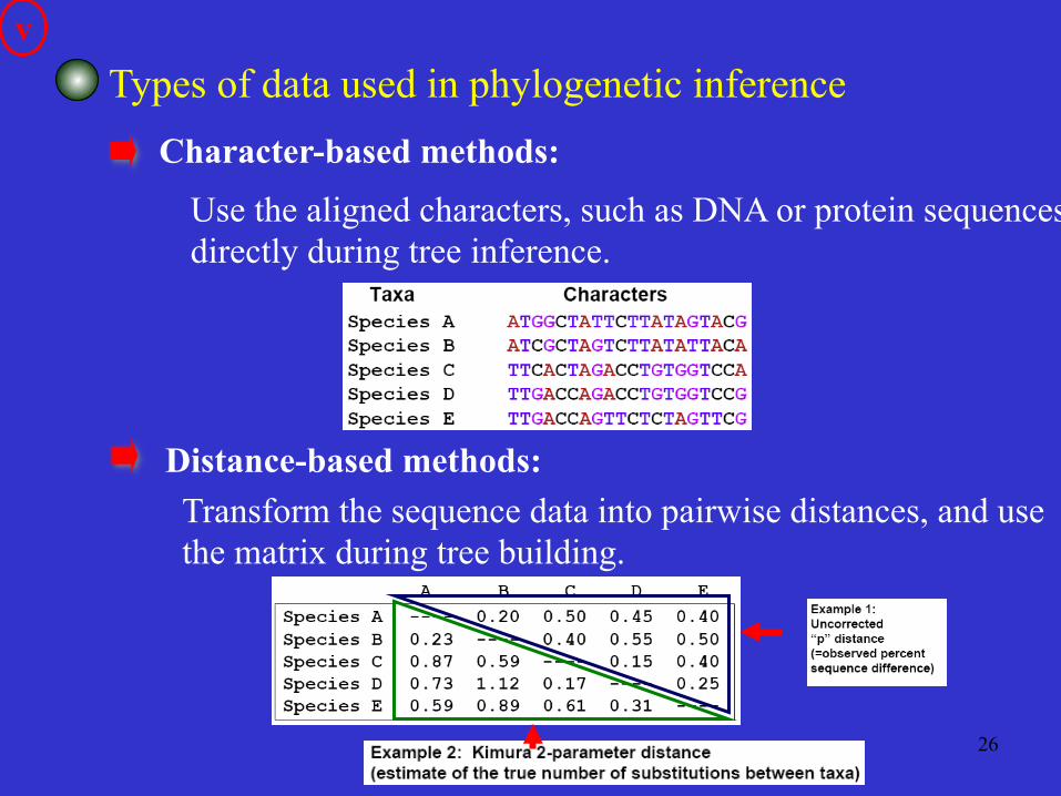
Types of data used in phylogenetic inference

Use the aligned characters, such as DNA or protein sequences, directly during tree inference.

Character-based methods:

Transform the sequence data into pairwise distances, and use the matrix during tree building.

Distance-based methods:

v

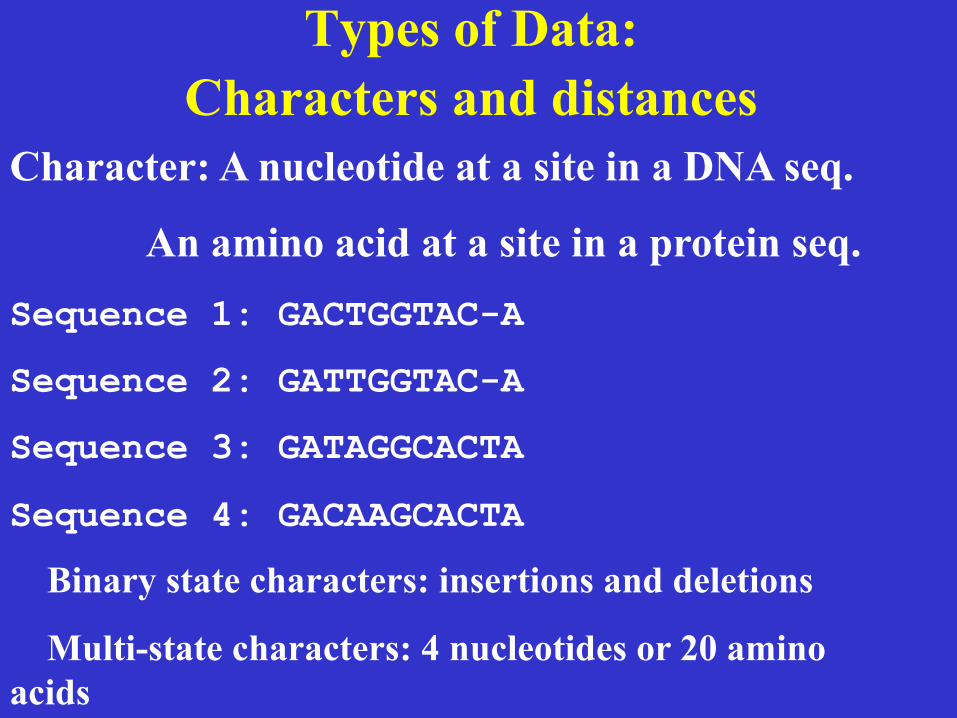
Types of Data: Characters and distances

Character: A nucleotide at a site in a DNA seq.

An amino acid at a site in a protein seq. Sequence 1: GACTGGTAC-A

Sequence 2: GATTGGTAC-A

Sequence 3: GATAGGCACTA

Sequence 4: GACAAGCACTA

Binary state characters: insertions and deletions

Multi-state characters: 4 nucleotides or 20 amino acids

Distance Matrix Methods

The evolutionary distances for all pairs of taxa are presented in a matrix.

Algorithms based on some functional relationships among the distance values

29

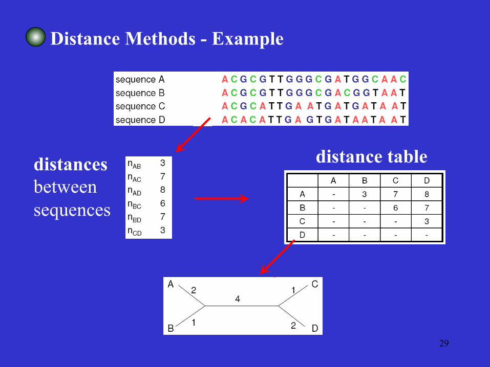
Distance Methods - Example

distances between sequences

distance table

Distance-based method

Unweighted Pair-Group Method with Arithmetic Mean

(UPGMA)

Unweighted Pair-Group Method with Arithmetic Mean

(UPGMA)

Sequential clustering algorithm

Local topological relationships are inferred in order of decreasing similarity and a phylogenetic tree is built in a stepwise manner.

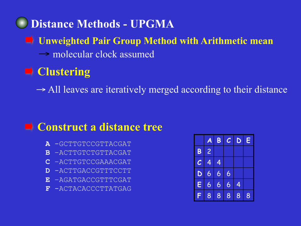
Distance Methods - UPGMA

Construct a distance tree A -GCTTGTCCGTTACGAT B –ACTTGTCTGTTACGAT C –ACTTGTCCGAAACGAT D -ACTTGACCGTTTCCTT E –AGATGACCGTTTCGAT F -ACTACACCCTTATGAG

A B C D E B 2C 4 4D 6 6 6E 6 6 6 4F 8 8 8 8 8

Clustering → All leaves are iteratively merged according to their distance

Unweighted Pair Group Method with Arithmetic mean → molecular clock assumed

33

Molecular Clocks

Amount of genetic difference between sequences is statistically proportional to the time since separation

→ The rate of evolution in a given protein (or DNA) molecule is approximately constant over time and among evolutionary lineages

→

The Molecular Clock Hypothesis

Proposed by Zuckerkandl and Pauling (1965) →

v v

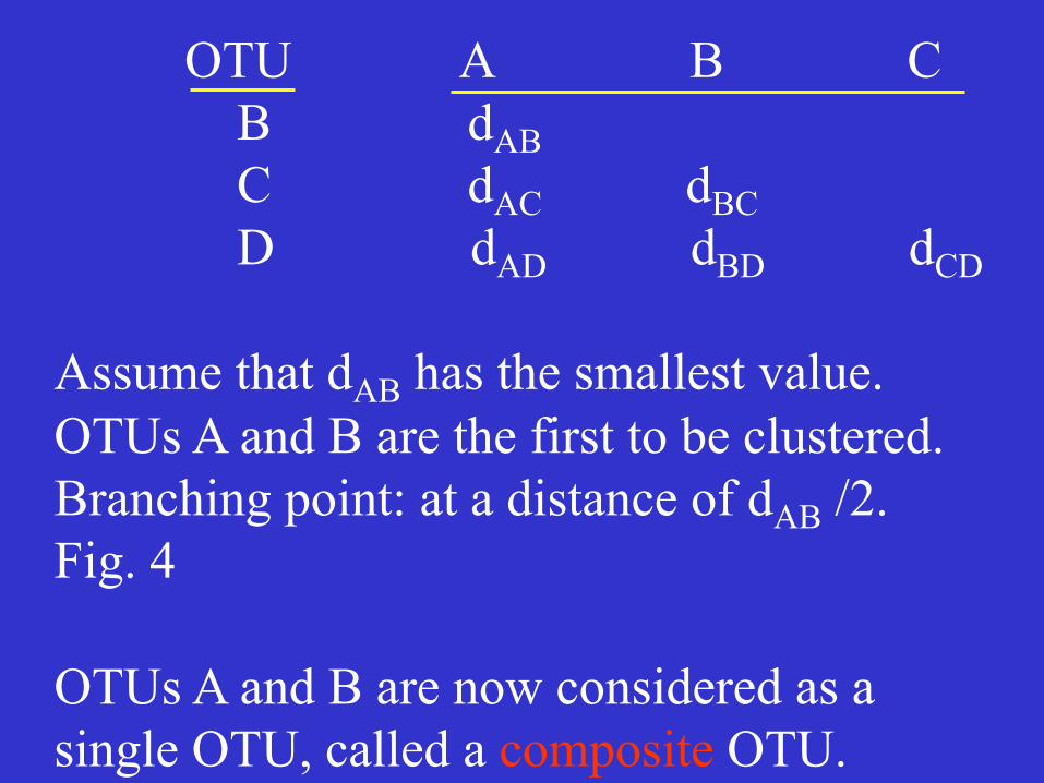
OTU A B C B dAB C dAC dBC D dAD dBD dCD Assume that dAB has the smallest value. OTUs A and B are the first to be clustered. Branching point: at a distance of dAB /2. Fig. 4 OTUs A and B are now considered as a single OTU, called a composite OTU.

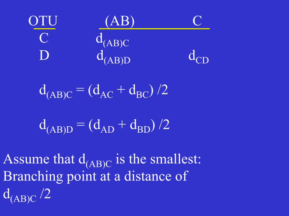
OTU (AB) C C d(AB)C D d(AB)D dCD d(AB)C = (dAC + dBC) /2 d(AB)D = (dAD + dBD) /2 Assume that d(AB)C is the smallest: Branching point at a distance of d(AB)C /2

A

B

C

D A

B

C

A

B

(a)

(b)

(c)

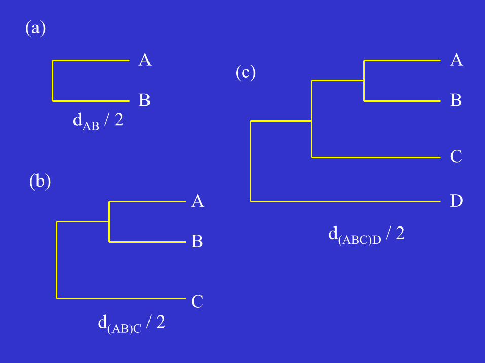
dAB / 2

d(AB)C / 2

d(ABC)D / 2

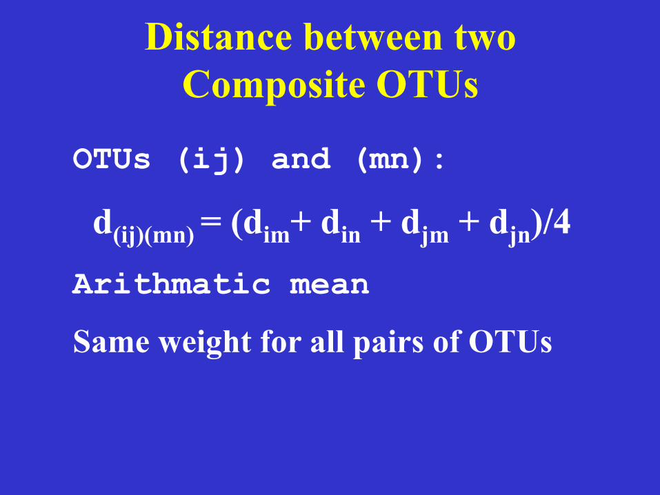
Distance between two Composite OTUs

OTUs (ij) and (mn):

d(ij)(mn) = (dim+ din + djm + djn)/4 Arithmatic mean

Same weight for all pairs of OTUs

38

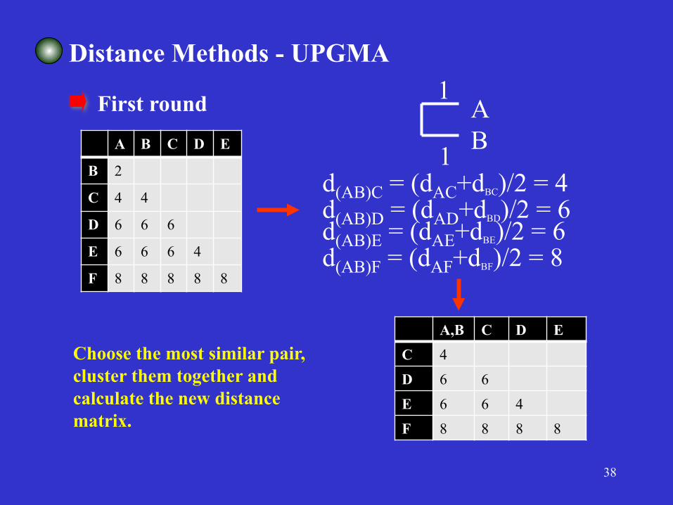
Distance Methods - UPGMA

First round

A B C D E

B 2

C 4 4

D 6 6 6

E 6 6 6 4

F 8 8 8 8 8

A B

1

1

A,B C D E C 4 D 6 6 E 6 6 4 F 8 8 8 8

Choose the most similar pair, cluster them together and calculate the new distance matrix.

d(AB)C = (dAC+dBC)/2 = 4 d(AB)D = (dAD+dBD)/2 = 6 d(AB)E = (dAE+dBE)/2 = 6 d(AB)F = (dAF+dBF)/2 = 8

39

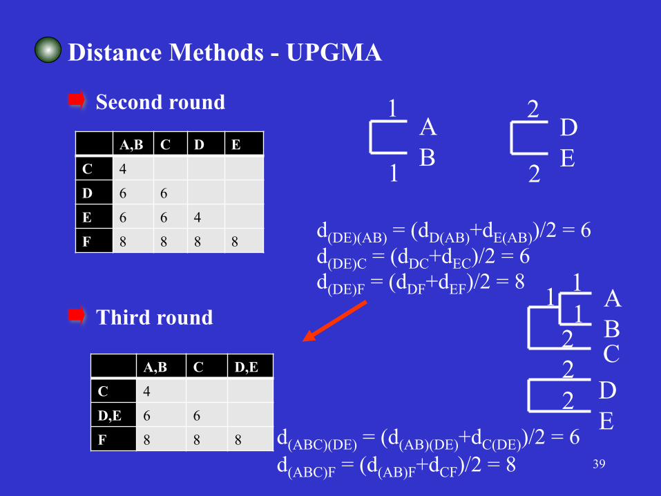
Distance Methods - UPGMA

Second round

A,B C D E C 4 D 6 6 E 6 6 4 F 8 8 8 8

Third round A B

1 1

A,B C D,E C 4 D,E 6 6 F 8 8 8

D E

2 2

C

1 2

d(DE)(AB) = (dD(AB)+dE(AB))/2 = 6 d(DE)C = (dDC+dEC)/2 = 6 d(DE)F = (dDF+dEF)/2 = 8

d(ABC)(DE) = (d(AB)(DE)+dC(DE))/2 = 6 d(ABC)F = (d(AB)F+dCF)/2 = 8

A B

1

1

D E

2

2

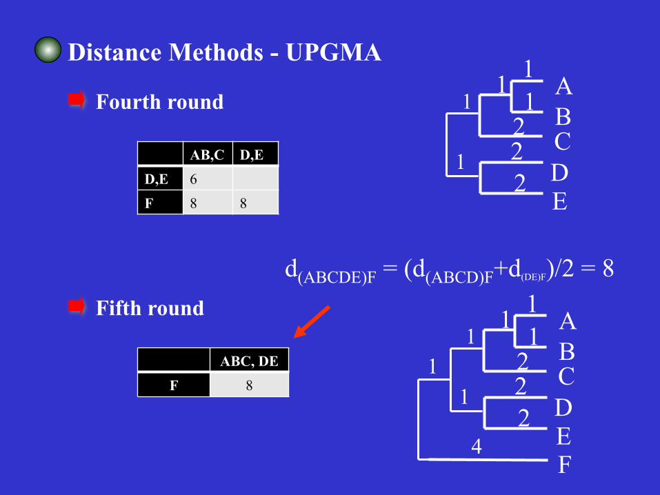
Distance Methods - UPGMA

Fourth round

AB,C D,E D,E 6 F 8 8

Fifth round

ABC, DE F 8

d(ABCDE)F = (d(ABCD)F+d(DE)F)/2 = 8

E

1

1

A B

1 1

C

1 2

D 2 2

E

1

1

A B

1 1

C

1 2

D 2 2

1

4 F

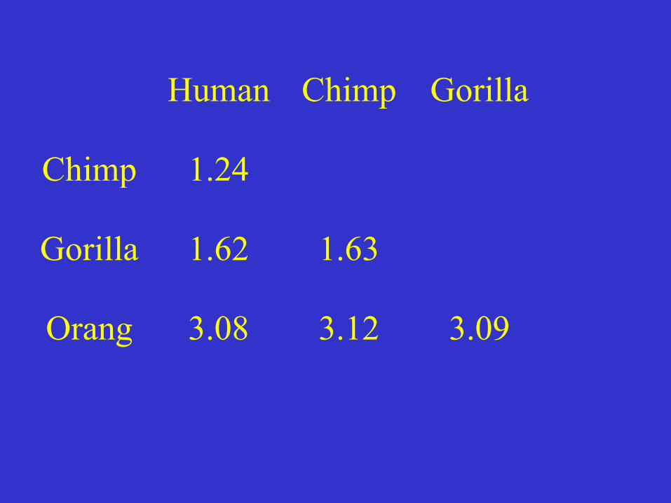
Human Chimp Gorilla

Chimp 1.24

Gorilla 1.62 1.63

Orang 3.08 3.12 3.09

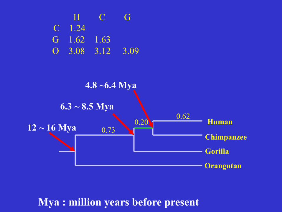
H C G C 1.24 G 1.62 1.63 O 3.08 3.12 3.09

0.62 0.20

0.73 Human

Chimpanzee

Gorilla

Orangutan

12 ~ 16 Mya

6.3 ~ 8.5 Mya

4.8 ~6.4 Mya

Mya : million years before present

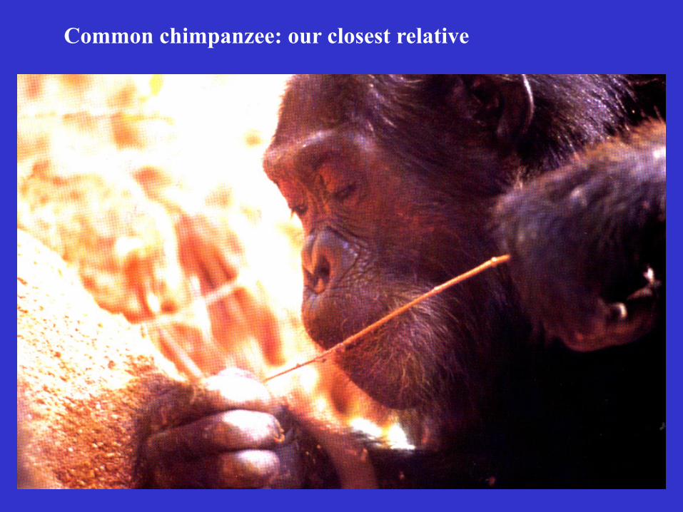
Common chimpanzee: our closest relative

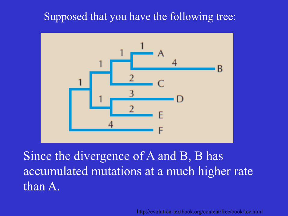
Supposed that you have the following tree:

Since the divergence of A and B, B has accumulated mutations at a much higher rate than A.

http://evolution-textbook.org/content/free/book/toc.html

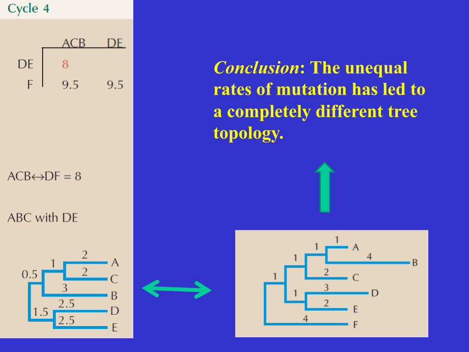
Conclusion: The unequal rates of mutation has led to a completely different tree topology.

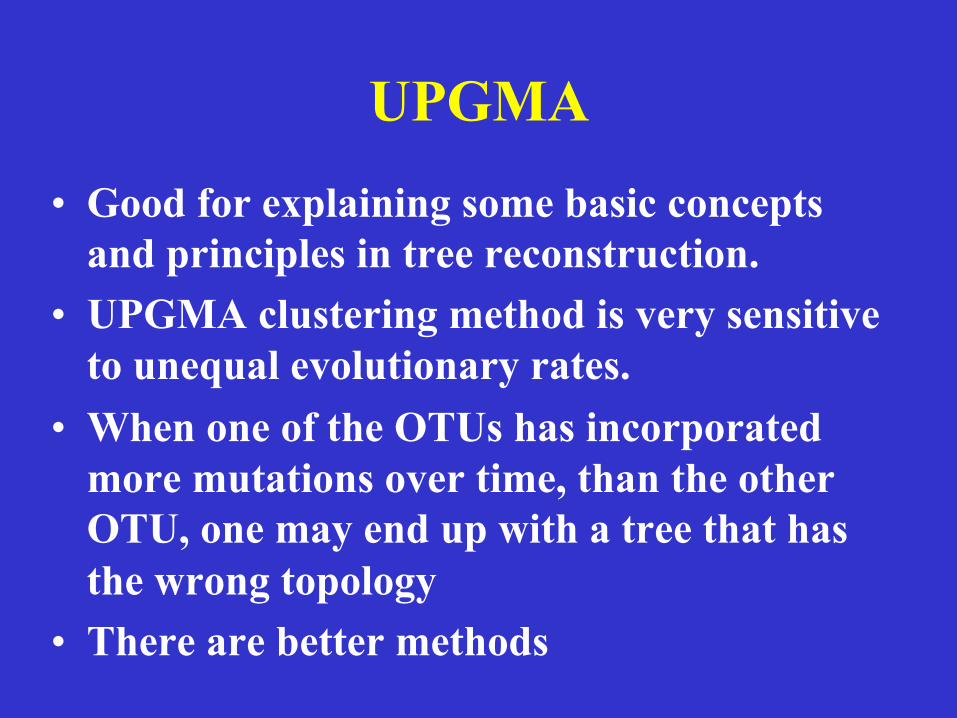
UPGMA •  Good for explaining some basic concepts

and principles in tree reconstruction. •  UPGMA clustering method is very sensitive

to unequal evolutionary rates. •  When one of the OTUs has incorporated

more mutations over time, than the other OTU, one may end up with a tree that has the wrong topology

•  There are better methods

Distance-based method

Neighbors-relation method

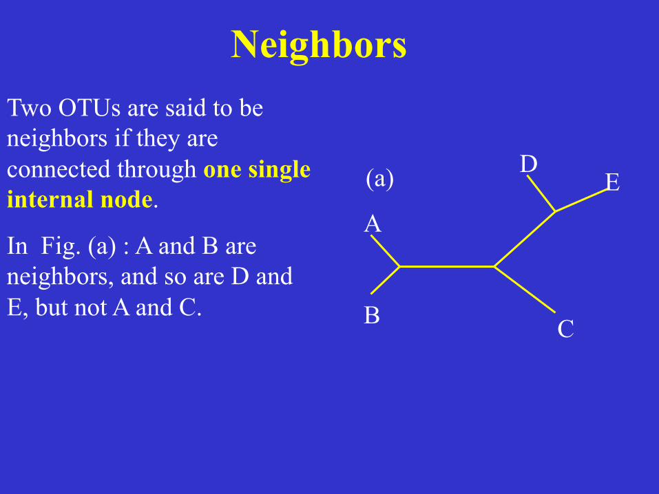
Neighbors Two OTUs are said to be neighbors if they are connected through one single internal node.

In Fig. (a) : A and B are neighbors, and so are D and E, but not A and C.

A

B C

D E(a)

(A B)

C

D E

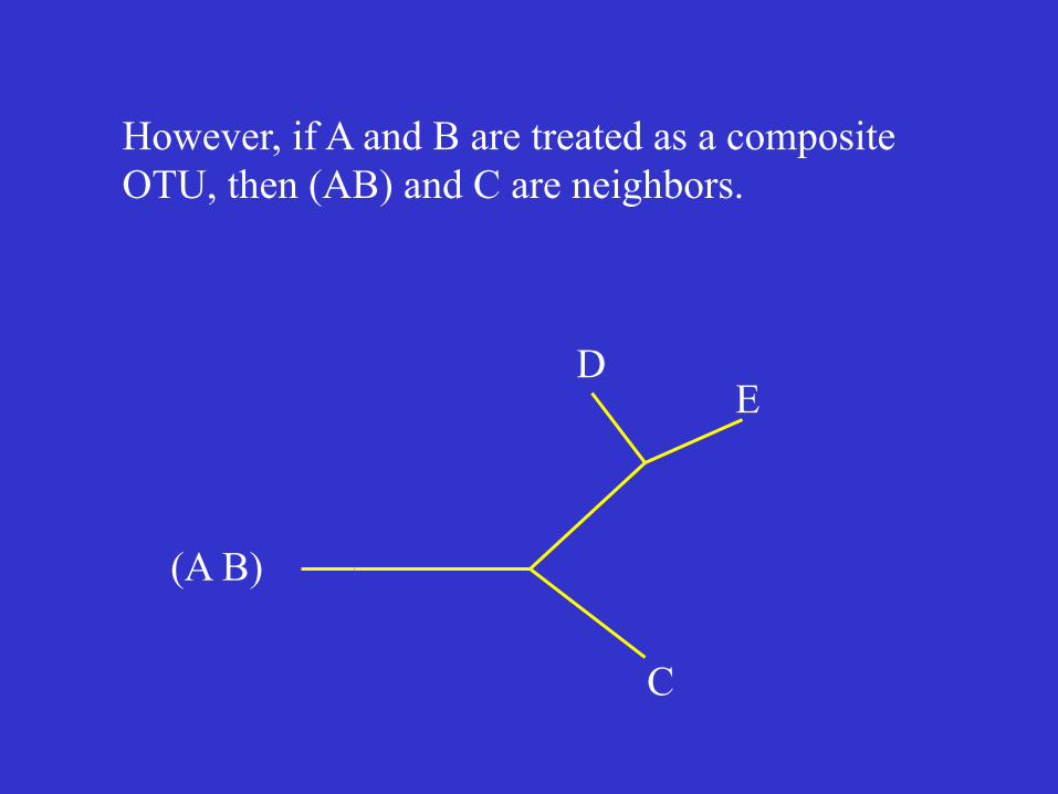
However, if A and B are treated as a composite OTU, then (AB) and C are neighbors.

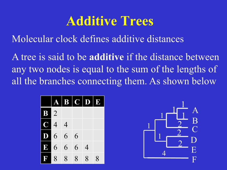
Additive Trees Molecular clock defines additive distances

A tree is said to be additive if the distance between any two nodes is equal to the sum of the lengths of all the branches connecting them. As shown below

A B C D E B 2 C 4 4 D 6 6 6 E 6 6 6 4 F 8 8 8 8 8

E

1

1

A B

1 1

C

1 2

D 2 2

1

4 F

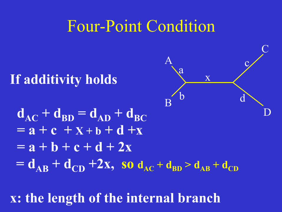
Four-Point Condition

If additivity holds dAC + dBD = dAD + dBC = a + c + X + b + d +x = a + b + c + d + 2x = dAB + dCD +2x, so dAC + dBD > dAB + dCD x: the length of the internal branch

A

B

C

D

x a

b

c

d

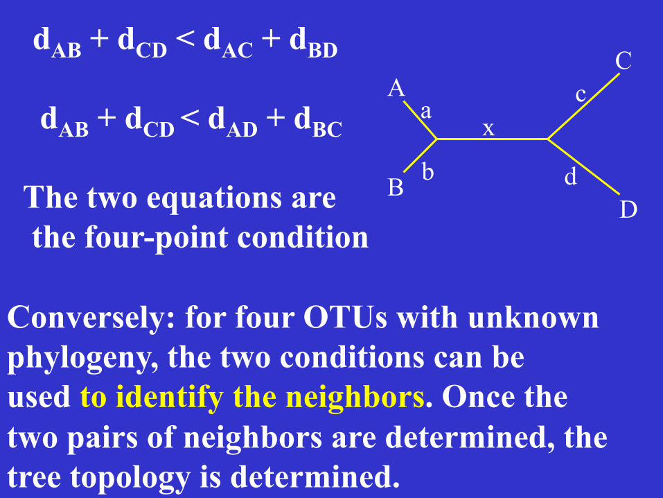
dAB + dCD < dAC + dBD dAB + dCD < dAD + dBC The two equations are the four-point condition Conversely: for four OTUs with unknown phylogeny, the two conditions can be used to identify the neighbors. Once the two pairs of neighbors are determined, the tree topology is determined.

A

B

C

D

x a

b

c

d

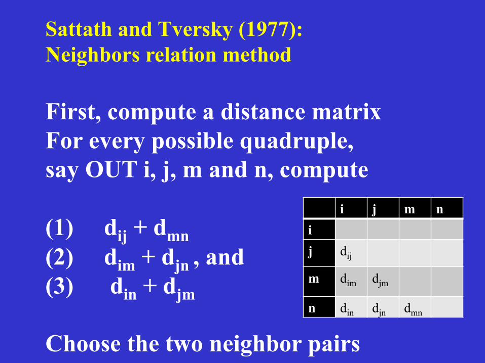
Sattath and Tversky (1977): Neighbors relation method First, compute a distance matrix For every possible quadruple, say OUT i, j, m and n, compute (1)   dij + dmn (2) dim + djn , and (3) din + djm Choose the two neighbor pairs

i j m n i j dij

m dim djm

n din djn dmn

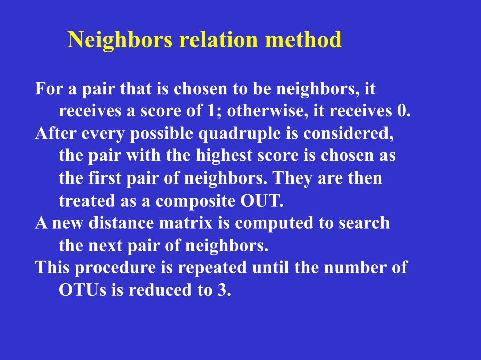
For a pair that is chosen to be neighbors, it receives a score of 1; otherwise, it receives 0.

After every possible quadruple is considered, the pair with the highest score is chosen as the first pair of neighbors. They are then treated as a composite OUT.

A new distance matrix is computed to search the next pair of neighbors.

This procedure is repeated until the number of OTUs is reduced to 3.

Neighbors relation method

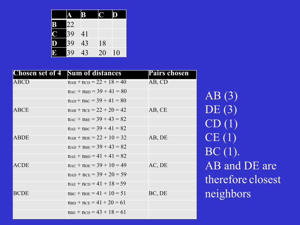
Chosen set of 4 Sum of distances Pairs chosen ABCD nAB + nCD = 22 + 18 = 40 AB, CD

nAC + nBD = 39 + 41 = 80 nAD

+ nBC = 39 + 41 = 80 ABCE nAB + nCE = 22 + 20 = 42 AB, CE

nAC + nBE = 39 + 43 = 82 nAE + nBC = 39 + 41 = 82

ABDE nAB + nDE = 22 + 10 = 32 AB, DE nAD + nBE = 39 + 43 = 82 nAE + nBD = 41 + 41 = 82

ACDE nAC + nDE = 39 + 10 = 49 AC, DE nAD + nCE = 39 + 20 = 59 nAE + nCD = 41 + 18 = 59

BCDE nBC + nDE = 41 + 10 = 51 BC, DE nBD + nCE = 41 + 20 = 61 nBE + nCD = 43 + 18 = 61

A B C D B 22 C 39 41 D 39 43 18 E 39 43 20 10

AB (3) DE (3) CD (1) CE (1) BC (1). AB and DE are therefore closest neighbors

Distance-based method

Neighbor-joining Method

Neighbor-joining Method

Minimum evolution tree: a tree with the smallest sum of branch lengths.

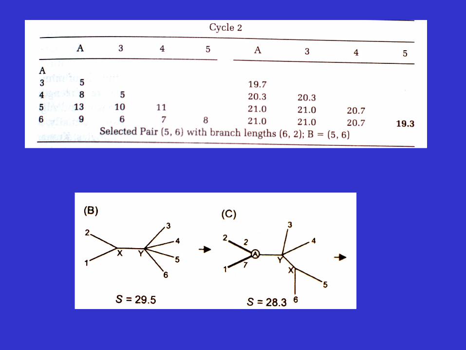
The neighbor-joining method finds neighbors sequentially that may minimize the total length of the tree.

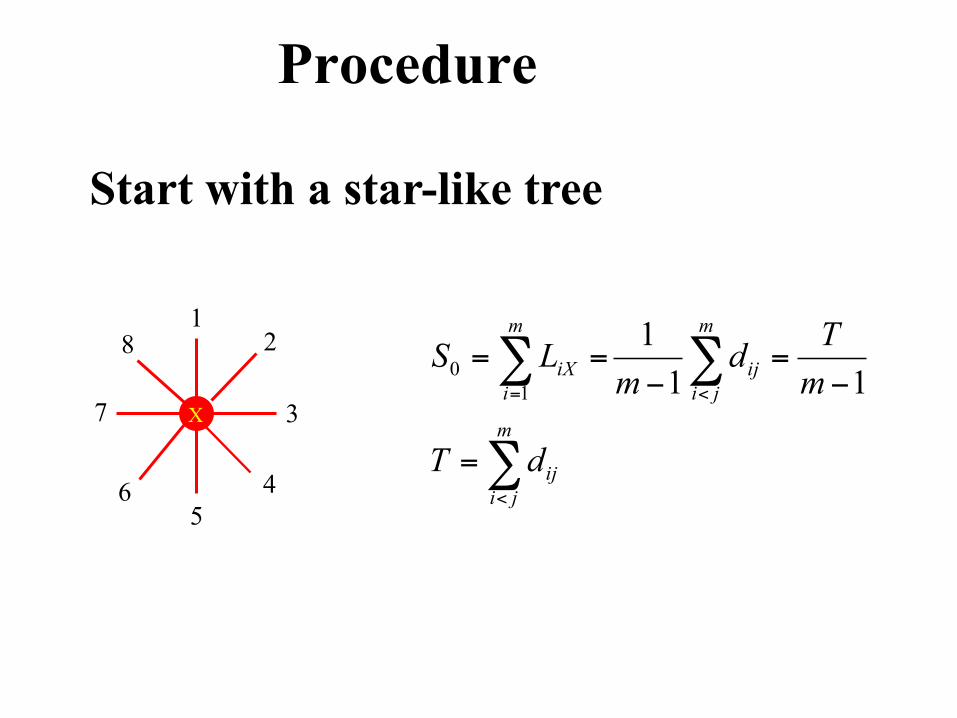
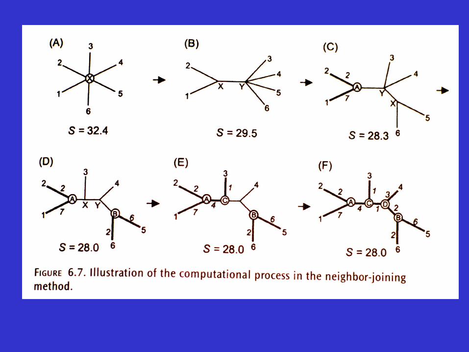
Procedure

Start with a star-like tree

X 7 3

5

1

4

8

6

2

∑

∑∑

<

<=

=

−=

−==

m

jiij

m

jiij

m

iiX

dT

mTd

mLS

111

10

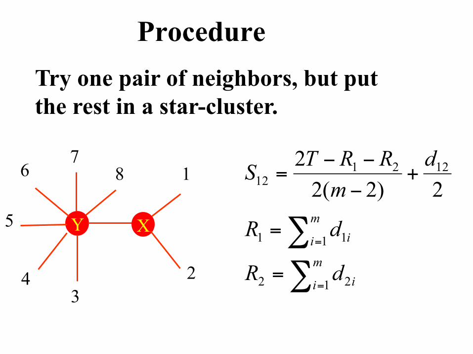
Procedure Try one pair of neighbors, but put the rest in a star-cluster.

∑∑

=

=

=

=

+−

−−=

m

i i

m

i i

dR

dR

dm

RRTS

1 22

1 11

122112 2)2(2

2

Y 5

3

7 6

4

8

2

1

X

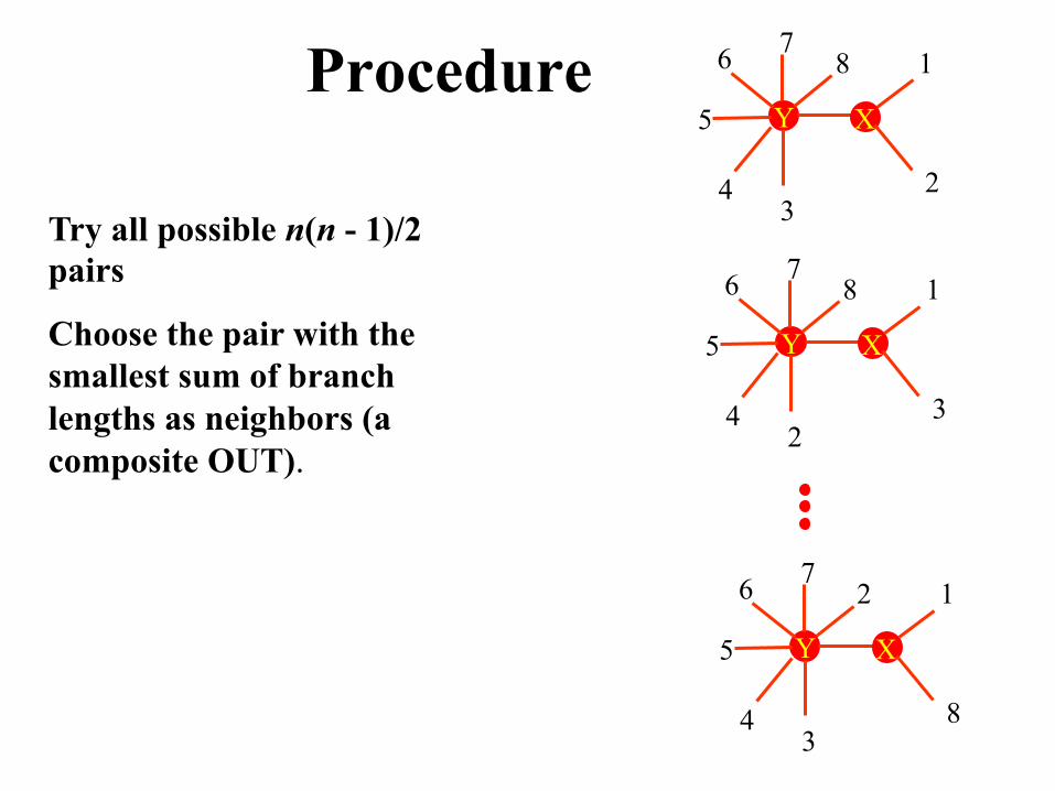
Procedure

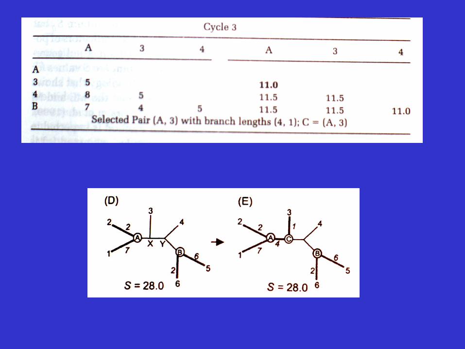
Try all possible n(n - 1)/2 pairs

Choose the pair with the smallest sum of branch lengths as neighbors (a composite OUT).

Y 5

3

7 6

4

8

2

1

X

Y 5

2

7 6

4

8

3

1

X

Y 5

3

7 6

4

2

8

1

X

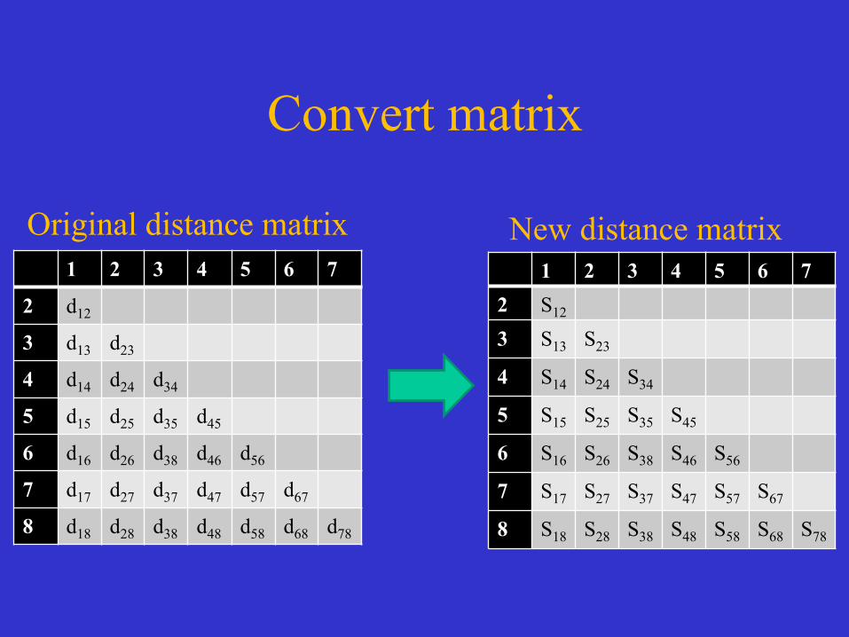
Convert matrix

1 2 3 4 5 6 7

2 d12

3 d13 d23

4 d14 d24 d34

5 d15 d25 d35 d45

6 d16 d26 d38 d46 d56

7 d17 d27 d37 d47 d57 d67

8 d18 d28 d38 d48 d58 d68 d78

Original distance matrix New distance matrix 1 2 3 4 5 6 7

2 S12

3 S13 S23

4 S14 S24 S34

5 S15 S25 S35 S45

6 S16 S26 S38 S46 S56

7 S17 S27 S37 S47 S57 S67

8 S18 S28 S38 S48 S58 S68 S78

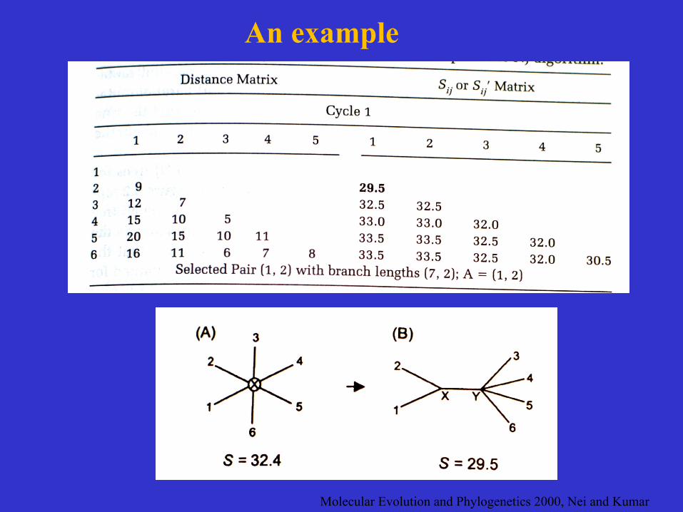
Molecular Evolution and Phylogenetics 2000, Nei and Kumar

An example

Advantages and disadvantages of the neighbor-joining method

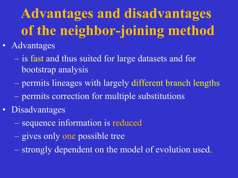
•  Advantages –  is fast and thus suited for large datasets and for

bootstrap analysis –  permits lineages with largely different branch lengths –  permits correction for multiple substitutions

•  Disadvantages –  sequence information is reduced –  gives only one possible tree –  strongly dependent on the model of evolution used.

Character-based method

Maximum Parsimony Method

Maximum Parsimony Method

Uses character state data

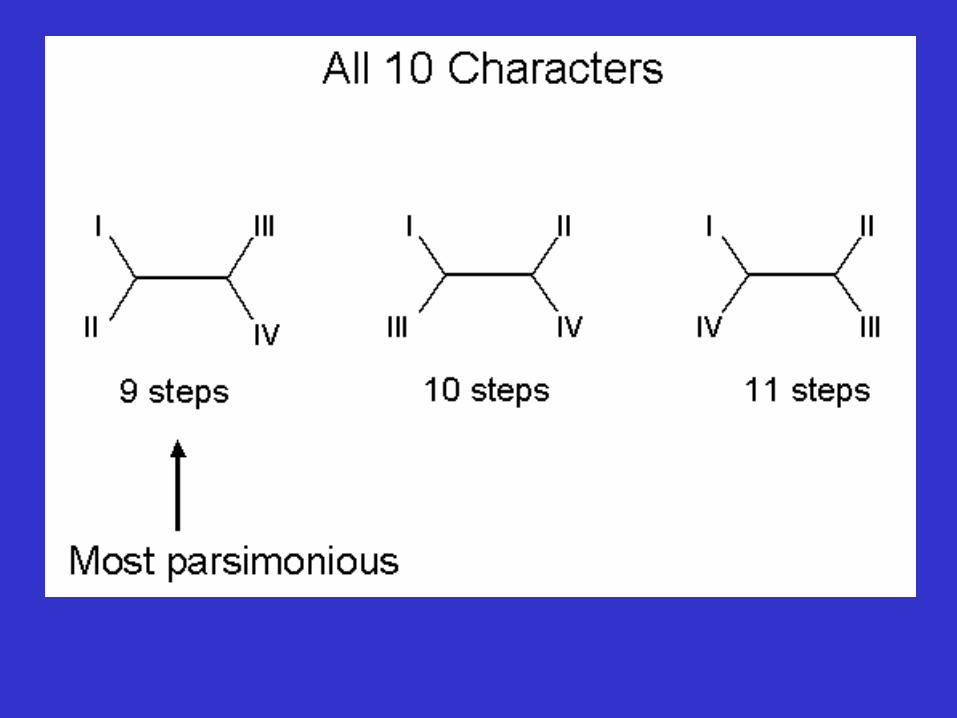
Search for a tree that requires the smallest number of evolutionary changes to explain the data.

A tree thus inferred is called the maximum parsimony tree

Maximum Parsimony Methods •  Using character state data for a given multiple

sequence alignment •  Give a score to a phylogenetic tree •  The score is a measure of the number of

evolutionary changes that would be required to generate the data given that particular tree.

•  Of the possible trees, the one considered most likely to represent the true history of the OTUs is the one with the lowest score (i.e., the one requiring the fewest evolutionary changes). A tree thus inferred is called the maximum parsimony tree

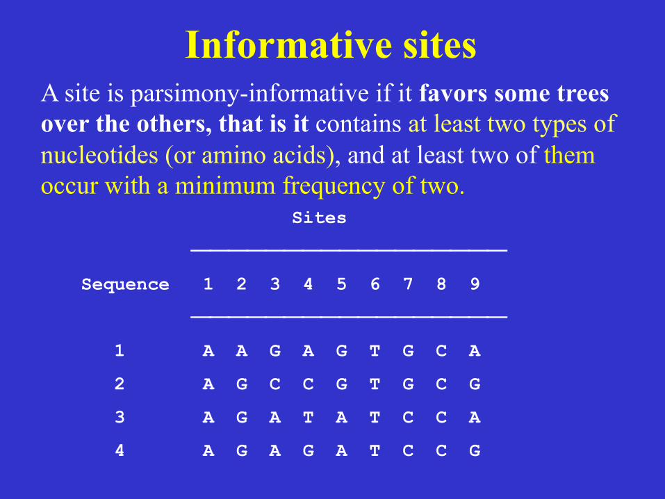
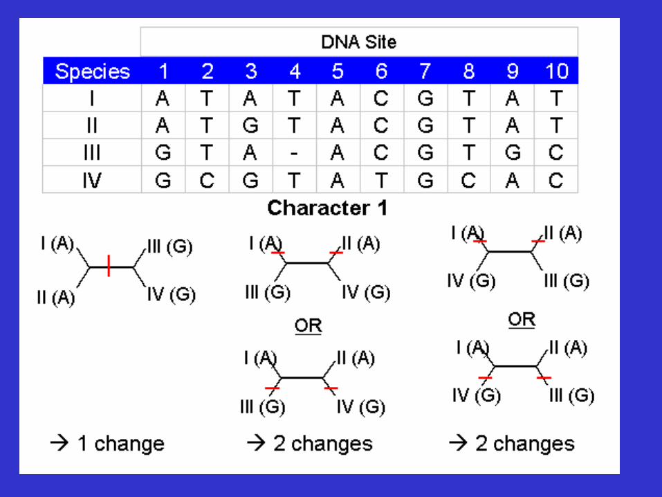
Informative sites A site is parsimony-informative if it favors some trees over the others, that is it contains at least two types of nucleotides (or amino acids), and at least two of them occur with a minimum frequency of two.

Sites

⎯⎯⎯⎯⎯⎯⎯⎯⎯⎯⎯⎯⎯⎯⎯⎯⎯

Sequence 1 2 3 4 5 6 7 8 9

⎯⎯⎯⎯⎯⎯⎯⎯⎯⎯⎯⎯⎯⎯⎯⎯⎯

1 A A G A G T G C A

2 A G C C G T G C G

3 A G A T A T C C A

4 A G A G A T C C G

Sites

⎯⎯⎯⎯⎯⎯⎯⎯⎯⎯⎯⎯⎯⎯⎯⎯⎯

Sequence 1 2 3 4 5 6 7 8 9

⎯⎯⎯⎯⎯⎯⎯⎯⎯⎯⎯⎯⎯⎯⎯⎯⎯

1 A A G A G T G C A

2 A G C C G T G C G

3 A G A T A T C C A

4 A G A G A T C C G

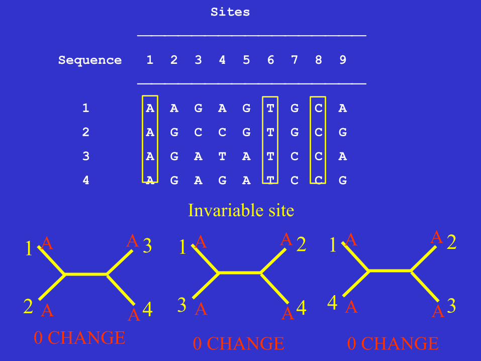
Invariable site

2

1 3

4

A

A

A

A 4

1 2

3

A

A

A

A 3

1 2

4

A

A

A

A 0 CHANGE 0 CHANGE 0 CHANGE

Sites

⎯⎯⎯⎯⎯⎯⎯⎯⎯⎯⎯⎯⎯⎯⎯⎯⎯

Sequence 1 2 3 4 5 6 7 8 9

⎯⎯⎯⎯⎯⎯⎯⎯⎯⎯⎯⎯⎯⎯⎯⎯⎯

1 A A G A G T G C A

2 A G C C G T G C G

3 A G A T A T C C A

4 A G A G A T C C G

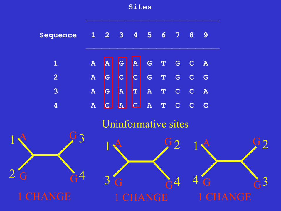
Uninformative sites

2

1 3

4

A

G

G

G 4

1 2

3

A

G

G

G 3

1 2

4

A

G

G

G 1 CHANGE 1 CHANGE 1 CHANGE

Sites

⎯⎯⎯⎯⎯⎯⎯⎯⎯⎯⎯⎯⎯⎯⎯⎯⎯

Sequence 1 2 3 4 5 6 7 8 9

⎯⎯⎯⎯⎯⎯⎯⎯⎯⎯⎯⎯⎯⎯⎯⎯⎯

1 A A G A G T G C A

2 A G C C G T G C G

3 A G A T A T C C A

4 A G A G A T C C G

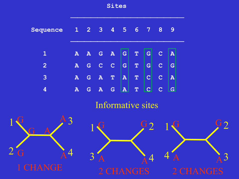
Informative sites

2

1 3

4

G

G

A

A

G A

4

1 2

3

G

A

G

A 3

1 2

4

G

A

G

A 1 CHANGE 2 CHANGES 2 CHANGES

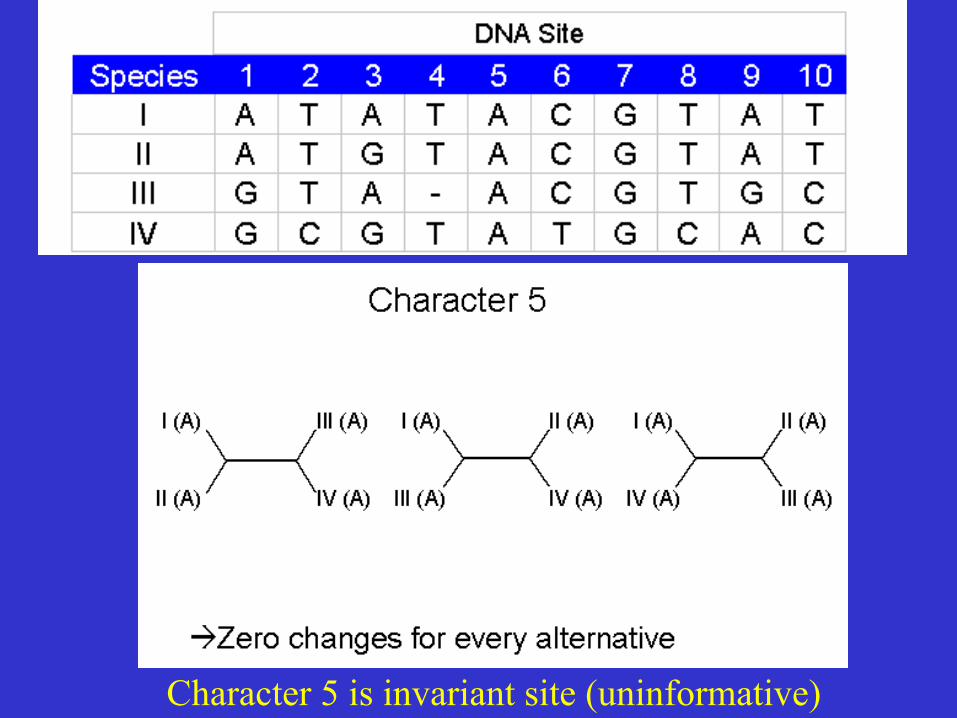
Character 5 is invariant site (uninformative)

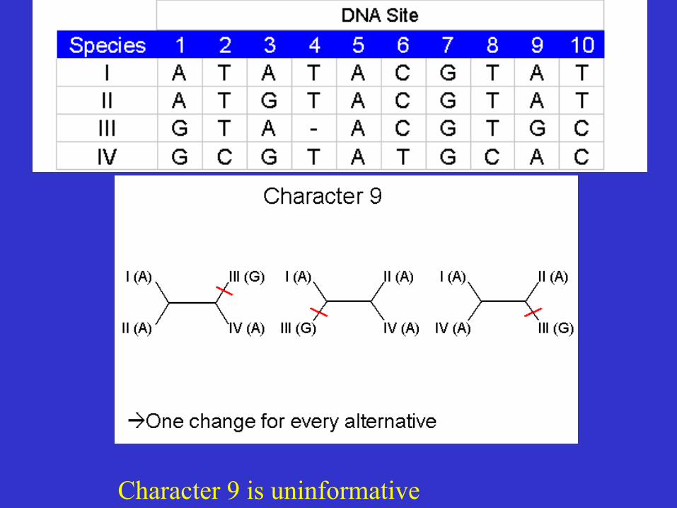
Character 9 is uninformative

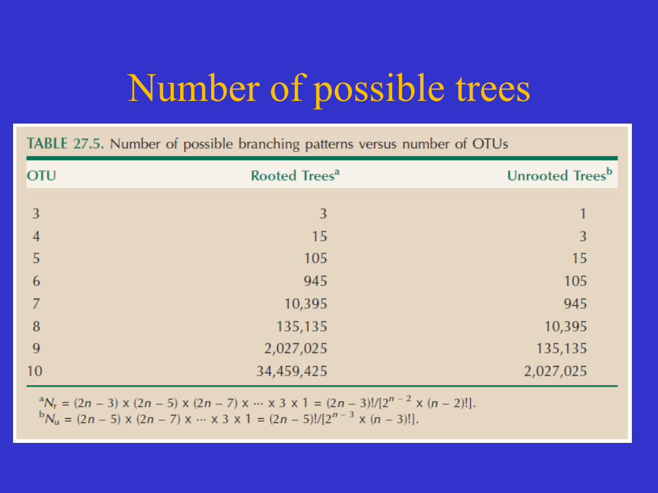
Number of possible trees

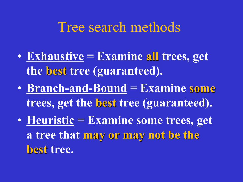
Tree search methods

•  Exhaustive = Examine all trees, get the best tree (guaranteed).

•  Branch-and-Bound = Examine some trees, get the best tree (guaranteed).

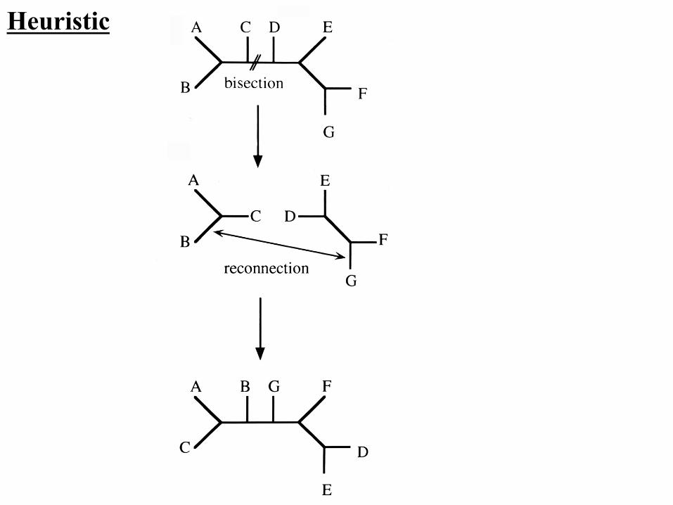
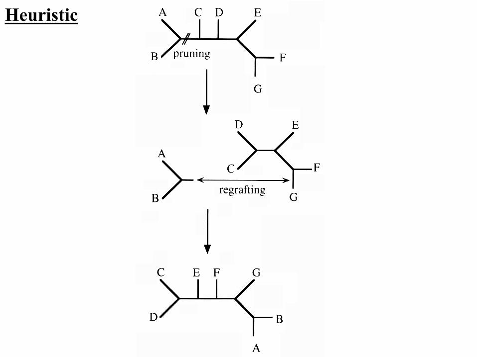
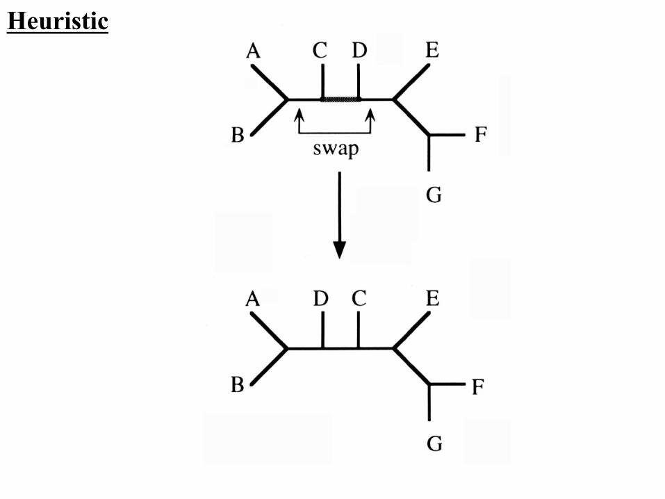
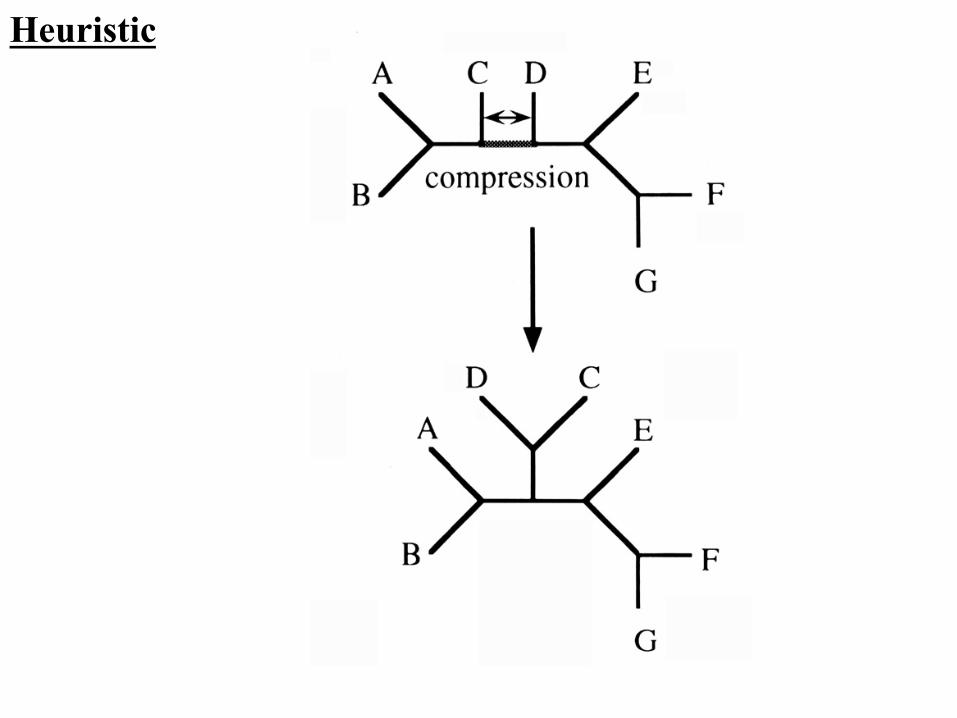
•  Heuristic = Examine some trees, get a tree that may or may not be the best tree.

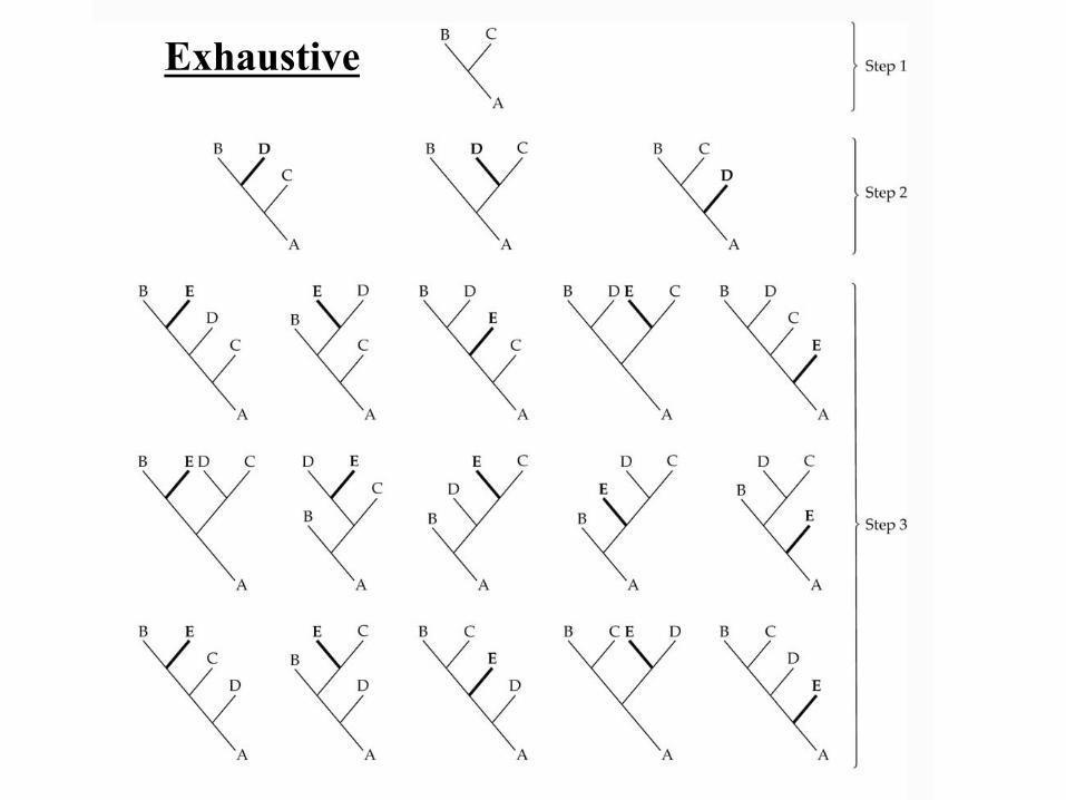
Exhaustive

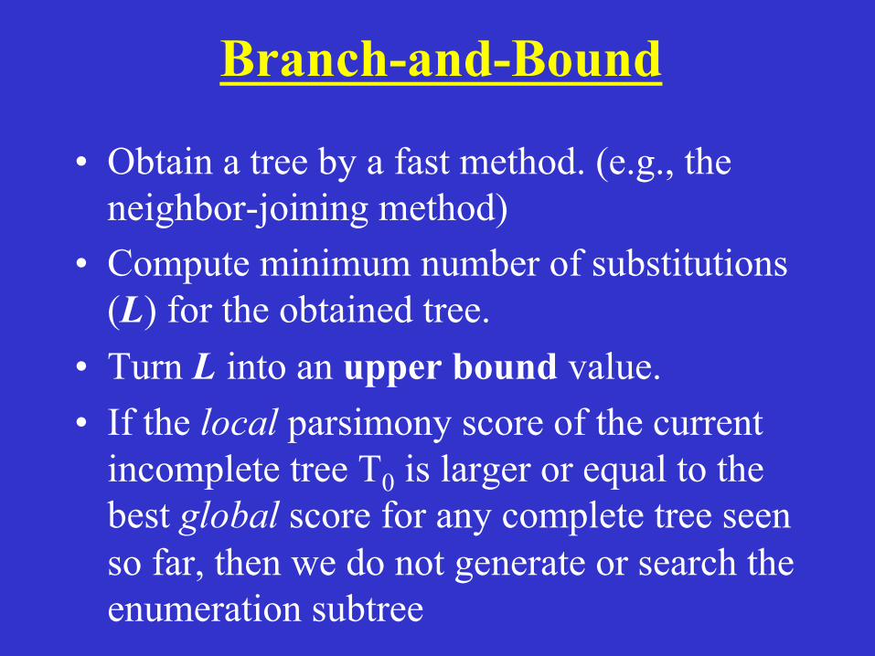
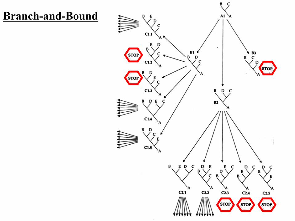
Branch-and-Bound

•  Obtain a tree by a fast method. (e.g., the neighbor-joining method)

•  Compute minimum number of substitutions (L) for the obtained tree.

•  Turn L into an upper bound value. •  If the local parsimony score of the current

incomplete tree T0 is larger or equal to the best global score for any complete tree seen so far, then we do not generate or search the enumeration subtree

Branch-and-Bound

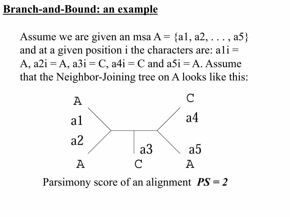
Assume we are given an msa A = {a1, a2, . . . , a5} and at a given position i the characters are: a1i = A, a2i = A, a3i = C, a4i = C and a5i = A. Assume that the Neighbor-Joining tree on A looks like this:

Branch-and-Bound: an example

Parsimony score of an alignment PS = 2

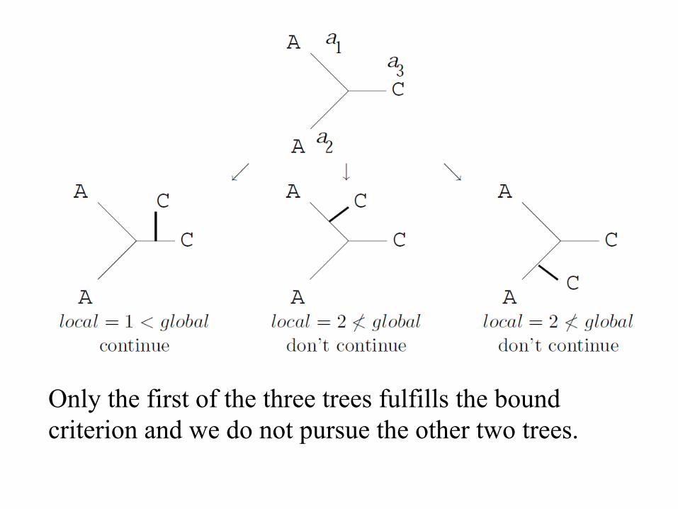
Only the first of the three trees fulfills the bound criterion and we do not pursue the other two trees.

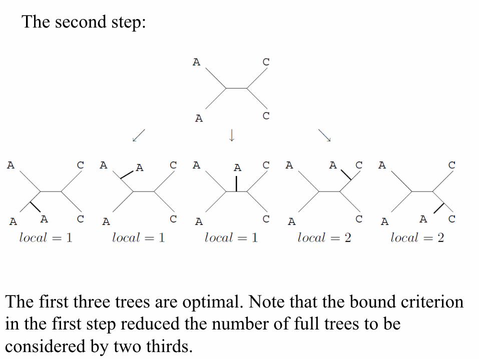
The second step:

The first three trees are optimal. Note that the bound criterion in the first step reduced the number of full trees to be considered by two thirds.

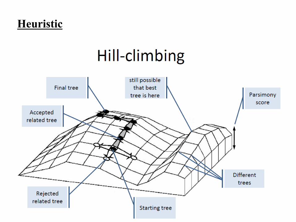
Heuristic

Heuristic

Heuristic

Heuristic

Heuristic

Maximum Likelihood Methods

Well-established approach in statistics

The ML method requires a probabilistic model for the process of nucleotide substitution. That is, we must specify the transition probability from one nucleotide state to another in a time interval in each branch.

Maximum Likelihood Method •  Likelihood provides probabilities of the

sequences given a model of their evolution on a particular tree.

•  The more probable the sequences given the tree, the more the tree is preferred.

•  All possible trees are considered; computationally intense.

•  Because the user can choose a model of evolution, the method can be useful for widely divergent groups or other difficult situations.

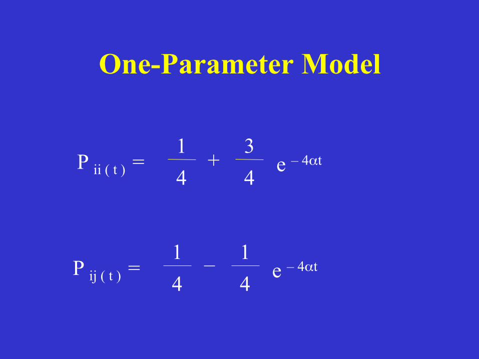
One-Parameter Model

P ii ( t ) = 4 1

4 3

+ e – 4αt

P ij ( t ) = 4 1

4 1 – e – 4αt

Likelihood function

Example:

Four sequences

A constant rate of substitution

x

y

z

t1

t2

t3

t 1 +

t 2+ t 3

t 2+ t 3

4 l

3 k

2 j

1 i

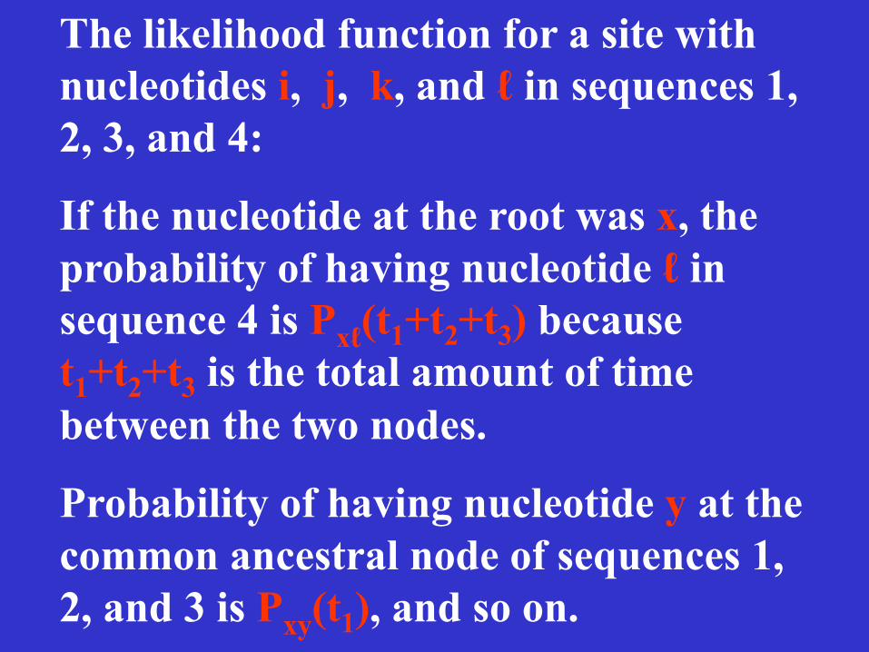
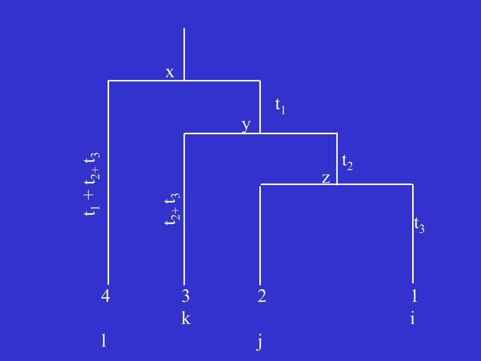
The likelihood function for a site with nucleotides i, j, k, and ℓ in sequences 1, 2, 3, and 4:

If the nucleotide at the root was x, the probability of having nucleotide ℓ in sequence 4 is Pxℓ(t1+t2+t3) because t1+t2+t3 is the total amount of time between the two nodes.

Probability of having nucleotide y at the common ancestral node of sequences 1, 2, and 3 is Pxy(t1), and so on.

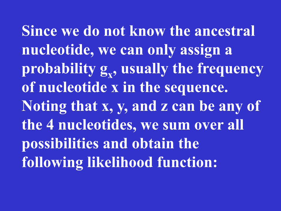
Since we do not know the ancestral nucleotide, we can only assign a probability gx, usually the frequency of nucleotide x in the sequence. Noting that x, y, and z can be any of the 4 nucleotides, we sum over all possibilities and obtain the following likelihood function:

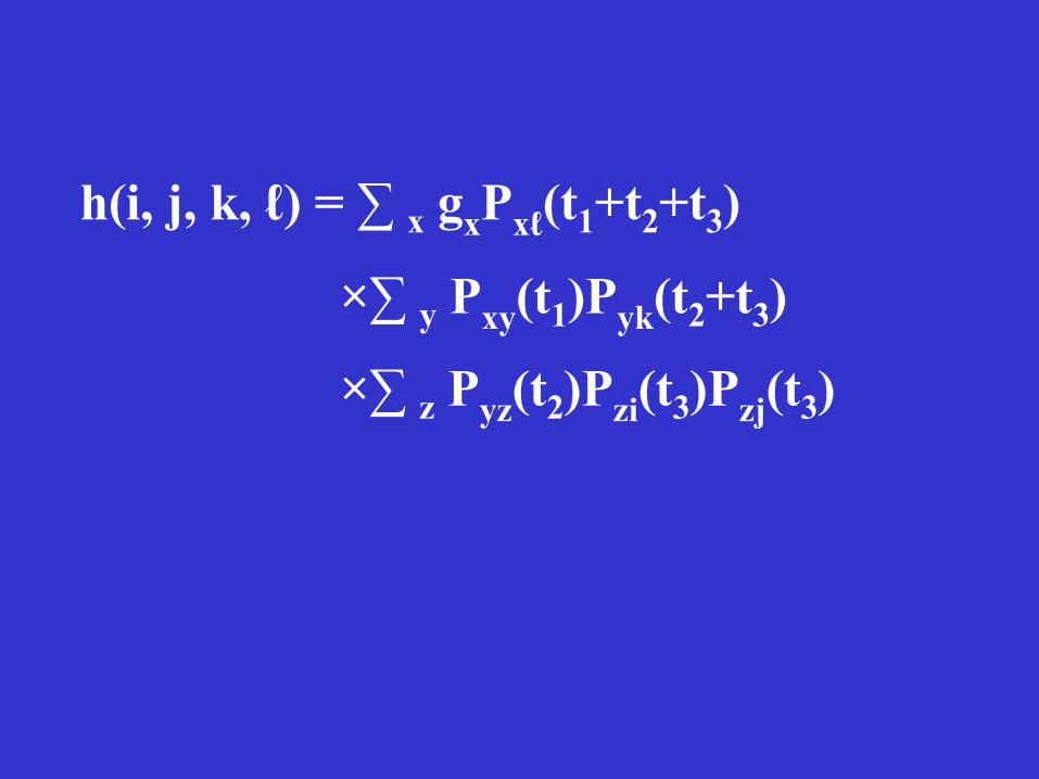
h(i, j, k, ℓ) = ∑ x gxPxℓ(t1+t2+t3)

×∑ y Pxy(t1)Pyk(t2+t3)

×∑ z Pyz(t2)Pzi(t3)Pzj(t3)

The above formula is for a single site. The likelihood for all sites is the product of the likelihoods for individual sites if all the nucleotide sites evolve independently.

For a given set of data, one computes the maximum likelihood value for each tree topology; this procedure is essentially to find the branch lengths that give the largest value for the likelihood function.

Finally, chooses the topology with the highest maximum likelihood value as the best tree, which is called the maximum likelihood tree.

Estimation of Branch Lengths Tree topology: Phylogenetic relationships

Branch lengths: Degree of separation

Topology and branch lengths are estimated at the same time:

UPGMA

Maximum parsimony

Maximum likelihood

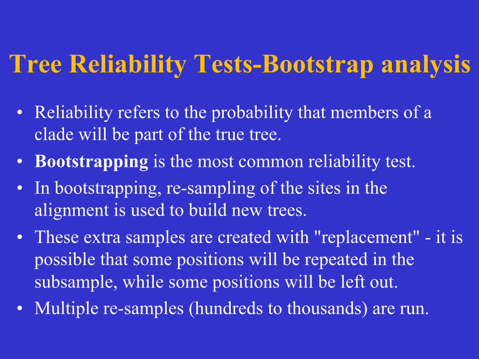
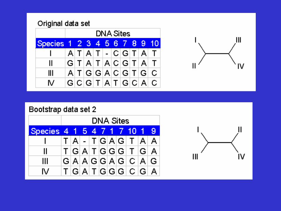
Tree Reliability Tests-Bootstrap analysis

•  Reliability refers to the probability that members of a clade will be part of the true tree.

•  Bootstrapping is the most common reliability test. •  In bootstrapping, re-sampling of the sites in the

alignment is used to build new trees. •  These extra samples are created with "replacement" - it is

possible that some positions will be repeated in the subsample, while some positions will be left out.

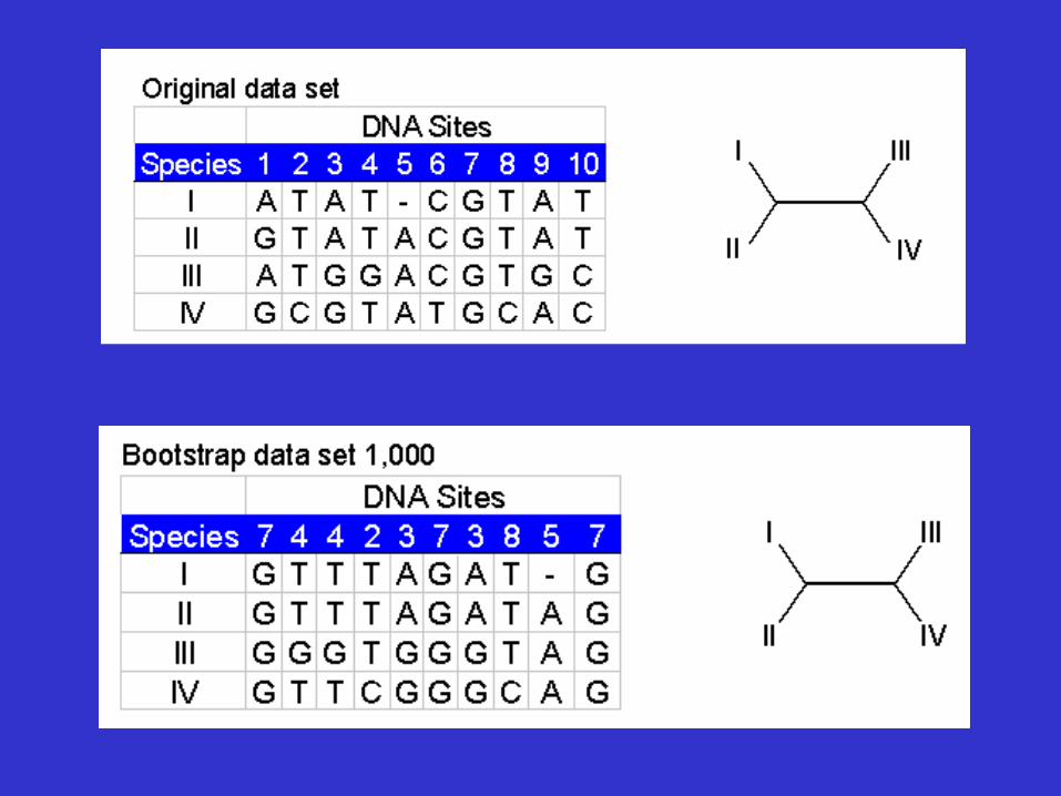
•  Multiple re-samples (hundreds to thousands) are run.

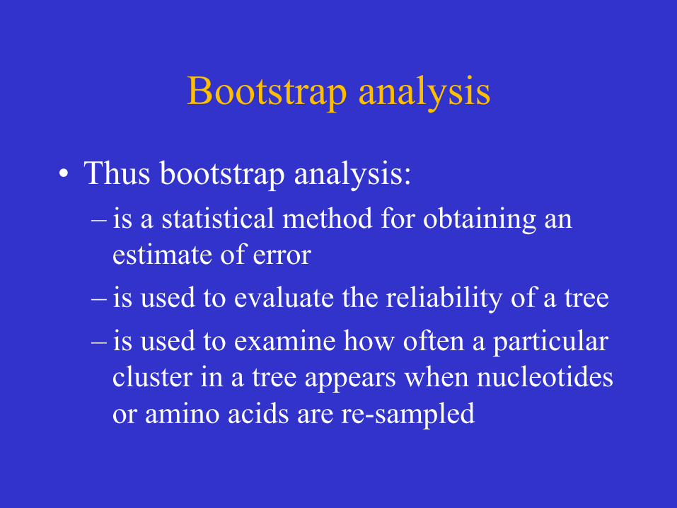
Bootstrap analysis

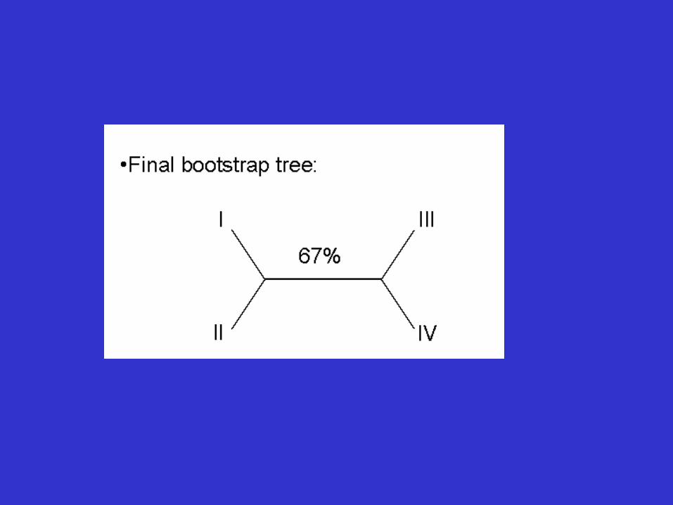
•  Thus bootstrap analysis: – is a statistical method for obtaining an

estimate of error – is used to evaluate the reliability of a tree – is used to examine how often a particular

cluster in a tree appears when nucleotides or amino acids are re-sampled

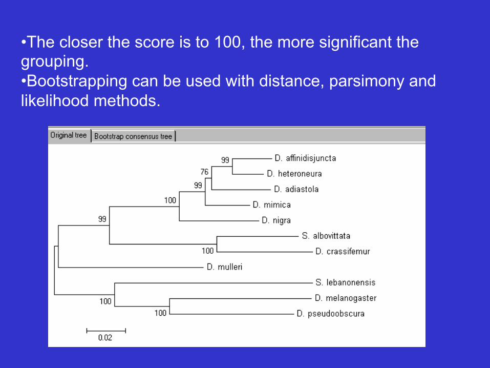
• The closer the score is to 100, the more significant the grouping. • Bootstrapping can be used with distance, parsimony and likelihood methods.

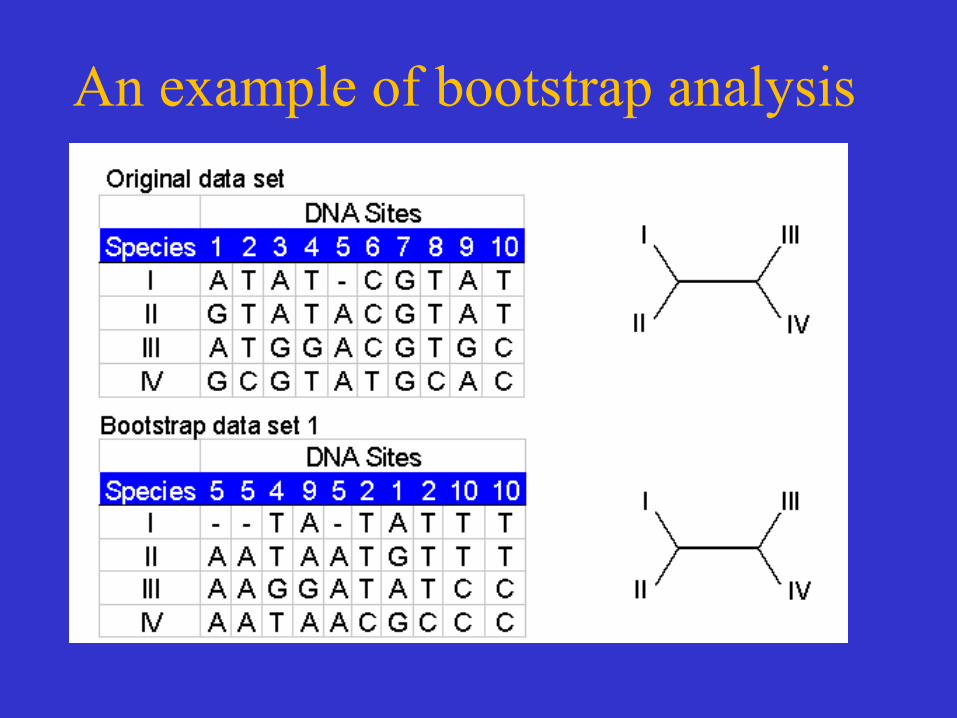
An example of bootstrap analysis

Bootstrap dataset 3 . . . . . . Bootstrap dataset 999