Spectral Analysis
125
Basic Definitions and The Spectral Estimation Problem Lecture 1 Lecture notes to accompany Introduction to Spectral Analysis Slide L1–1 by P. Stoica and R. Moses, Prentice Hall, 1997
description
Spectral Analysis by Petre Stoica
Transcript of Spectral Analysis
Basic Definitions
and
The Spectral Estimation Problem
Lecture 1
Lecture notes to accompany Introduction to Spectral Analysis Slide L1–1by P. Stoica and R. Moses, Prentice Hall, 1997
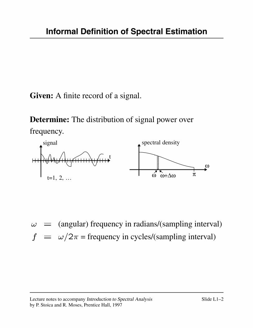
Informal Definition of Spectral Estimation
Given: A finite record of a signal.
Determine: The distribution of signal power over
frequency.
t
signal
t=1, 2, . . . ω ω+∆ωω
π
spectral density
! = (angular) frequency in radians/(sampling interval)
f = !=2� = frequency in cycles/(sampling interval)
Lecture notes to accompany Introduction to Spectral Analysis Slide L1–2by P. Stoica and R. Moses, Prentice Hall, 1997
Applications
Temporal Spectral Analysis
� Vibration monitoring and fault detection
� Hidden periodicity finding
� Speech processing and audio devices
� Medical diagnosis
� Seismology and ground movement study
� Control systems design
� Radar, Sonar
Spatial Spectral Analysis
� Source location using sensor arrays
Lecture notes to accompany Introduction to Spectral Analysis Slide L1–3by P. Stoica and R. Moses, Prentice Hall, 1997
Deterministic Signals
fy(t)g1t=�1 = discrete-time deterministic data
sequence
If:1X
t=�1
jy(t)j2 <1
Then: Y (!) =1X
t=�1
y(t)e�i!t
exists and is called the Discrete-Time Fourier Transform(DTFT)
Lecture notes to accompany Introduction to Spectral Analysis Slide L1–4by P. Stoica and R. Moses, Prentice Hall, 1997
Energy Spectral Density
Parseval's Equality:
1Xt=�1
jy(t)j2 =1
2�
Z ���
S(!)d!
where
S(!)4= jY (!)j2
= Energy Spectral Density
We can write
S(!) =1X
k=�1
�(k)e�i!k
where
�(k) =1X
t=�1
y(t)y�(t� k)
Lecture notes to accompany Introduction to Spectral Analysis Slide L1–5by P. Stoica and R. Moses, Prentice Hall, 1997

Random Signals
Random Signal
t
random signal probabilistic statements about future variations
current observation time
Here:1X
t=�1
jy(t)j2 =1
But: Enjy(t)j2
o<1
E f�g = Expectation over the ensemble of realizations
Enjy(t)j2
o= Average power in y(t)
PSD = (Average) power spectral density
Lecture notes to accompany Introduction to Spectral Analysis Slide L1–6by P. Stoica and R. Moses, Prentice Hall, 1997
First Definition of PSD
�(!) =1X
k=�1
r(k)e�i!k
where r(k) is the autocovariance sequence (ACS)
r(k) = E fy(t)y�(t� k)g
r(k) = r�(�k); r(0) � jr(k)j
Note that
r(k) =1
2�
Z ���
�(!)ei!kd! (Inverse DTFT)
Interpretation:
r(0) = Enjy(t)j2
o=
1
2�
Z ���
�(!)d!
so
�(!)d! = infinitesimal signal power in the band
! � d!2
Lecture notes to accompany Introduction to Spectral Analysis Slide L1–7by P. Stoica and R. Moses, Prentice Hall, 1997
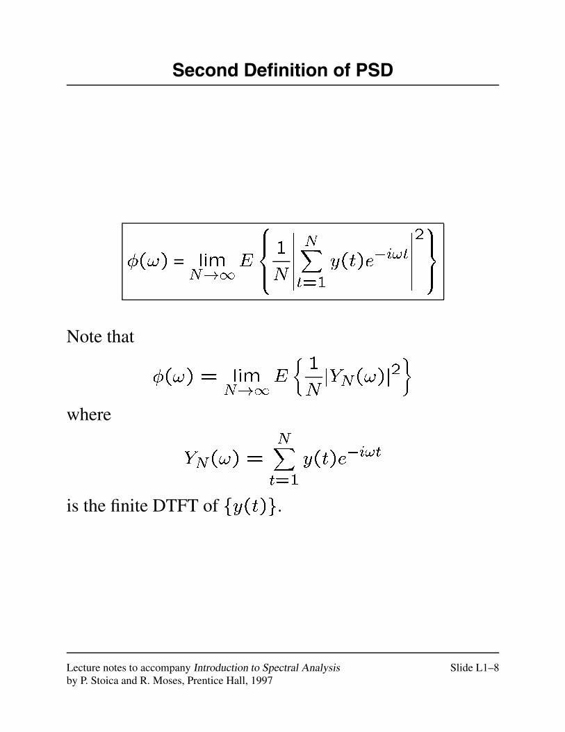
Second Definition of PSD
�(!) = limN!1
E
8><>:1
N
������NXt=1
y(t)e�i!t
������29>=>;
Note that
�(!) = limN!1
E
�1
NjYN(!)j
2�
where
YN(!) =NXt=1
y(t)e�i!t
is the finite DTFT of fy(t)g.
Lecture notes to accompany Introduction to Spectral Analysis Slide L1–8by P. Stoica and R. Moses, Prentice Hall, 1997
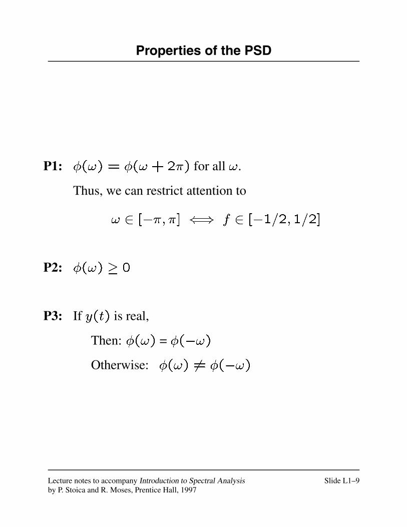
Properties of the PSD
P1: �(!) = �(!+2�) for all !.
Thus, we can restrict attention to
! 2 [��; �] () f 2 [�1=2;1=2]
P2: �(!) � 0
P3: If y(t) is real,
Then: �(!) = �(�!)
Otherwise: �(!) 6= �(�!)
Lecture notes to accompany Introduction to Spectral Analysis Slide L1–9by P. Stoica and R. Moses, Prentice Hall, 1997
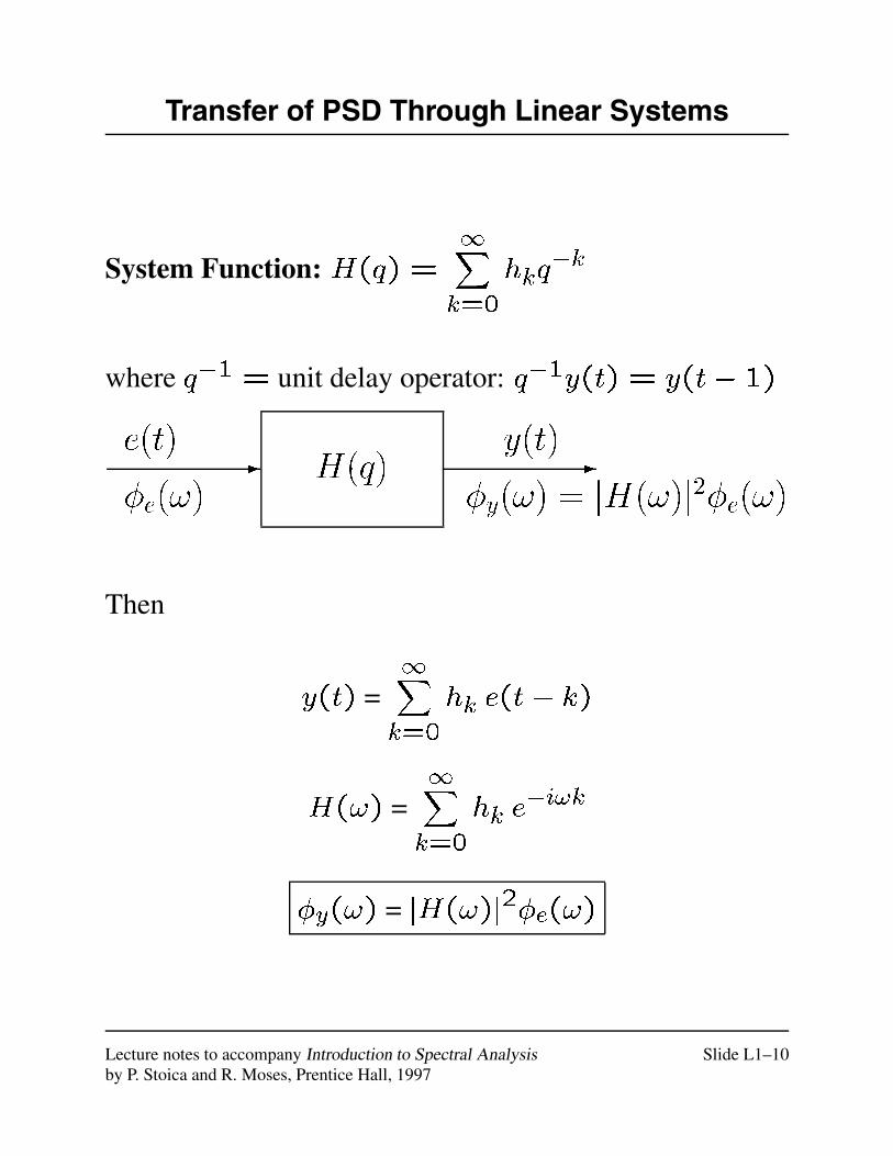
Transfer of PSD Through Linear Systems
System Function: H(q) =1Xk=0
hkq�k
where q�1 = unit delay operator: q�1y(t) = y(t� 1)
e(t)
�e(!)
y(t)
�y(!) = jH(!)j2�e(!)H(q) --
Then
y(t) =1Xk=0
hk e(t� k)
H(!) =1Xk=0
hk e�i!k
�y(!) = jH(!)j2�e(!)
Lecture notes to accompany Introduction to Spectral Analysis Slide L1–10by P. Stoica and R. Moses, Prentice Hall, 1997
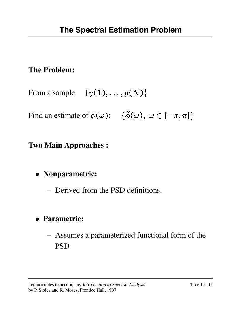
The Spectral Estimation Problem
The Problem:
From a sample fy(1); : : : ; y(N)g
Find an estimate of �(!): f�(!); ! 2 [��; �]g
Two Main Approaches :
� Nonparametric:
– Derived from the PSD definitions.
� Parametric:
– Assumes a parameterized functional form of the
PSD
Lecture notes to accompany Introduction to Spectral Analysis Slide L1–11by P. Stoica and R. Moses, Prentice Hall, 1997
Periodogram
and
Correlogram
Methods
Lecture 2
Lecture notes to accompany Introduction to Spectral Analysis Slide L2–1by P. Stoica and R. Moses, Prentice Hall, 1997
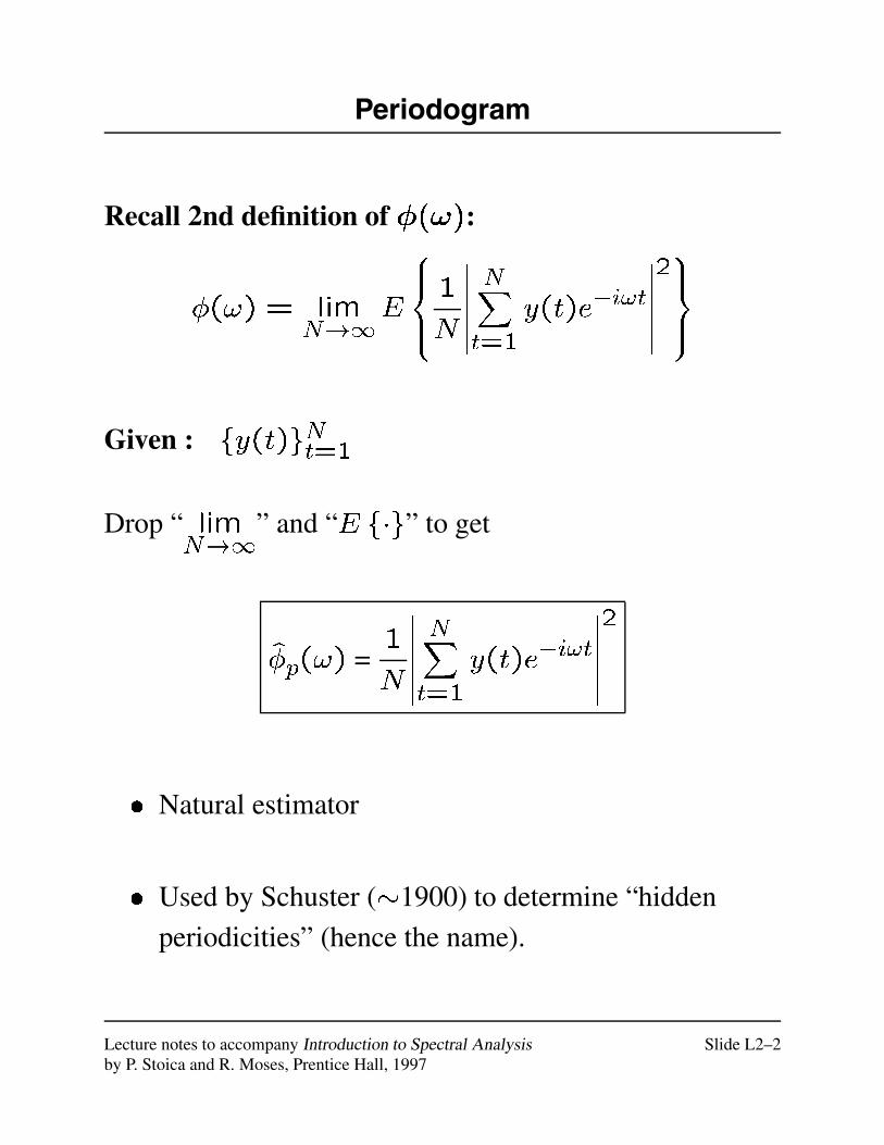
Periodogram
Recall 2nd definition of �(!):
�(!) = limN!1
E
8><>:1
N
������NXt=1
y(t)e�i!t
������29>=>;
Given : fy(t)gNt=1
Drop “ limN!1
” and “E f�g” to get
�p(!) =1
N
������NXt=1
y(t)e�i!t
������2
� Natural estimator
� Used by Schuster (�1900) to determine “hidden
periodicities” (hence the name).
Lecture notes to accompany Introduction to Spectral Analysis Slide L2–2by P. Stoica and R. Moses, Prentice Hall, 1997
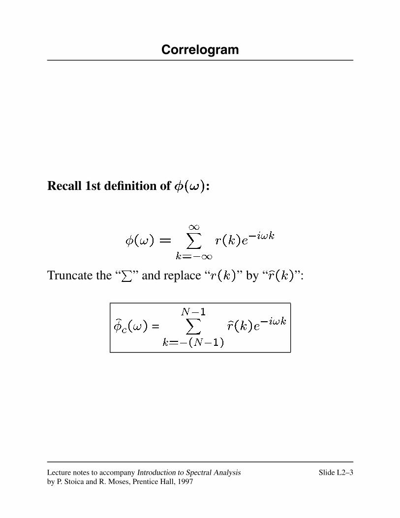
Correlogram
Recall 1st definition of �(!):
�(!) =1X
k=�1
r(k)e�i!k
Truncate the “P
” and replace “r(k)” by “r(k)”:
�c(!) =N�1X
k=�(N�1)
r(k)e�i!k
Lecture notes to accompany Introduction to Spectral Analysis Slide L2–3by P. Stoica and R. Moses, Prentice Hall, 1997
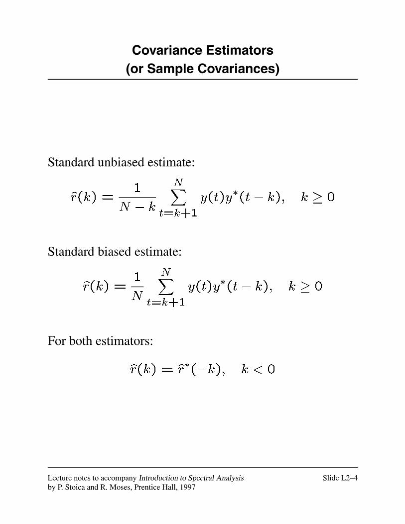
Covariance Estimators(or Sample Covariances)
Standard unbiased estimate:
r(k) =1
N � k
NXt=k+1
y(t)y�(t� k); k � 0
Standard biased estimate:
r(k) =1
N
NXt=k+1
y(t)y�(t� k); k � 0
For both estimators:
r(k) = r�(�k); k < 0
Lecture notes to accompany Introduction to Spectral Analysis Slide L2–4by P. Stoica and R. Moses, Prentice Hall, 1997
Relationship Between �p(!) and �c(!)
If: the biased ACS estimator r(k) is used in �c(!),
Then:
�p(!) =1
N
������NXt=1
y(t)e�i!t
������2
=N�1X
k=�(N�1)
r(k)e�i!k
= �c(!)
�p(!) = �c(!)
Consequence:Both �p(!) and �c(!) can be analyzed simultaneously.
Lecture notes to accompany Introduction to Spectral Analysis Slide L2–5by P. Stoica and R. Moses, Prentice Hall, 1997
Statistical Performance of �p(!) and �c(!)
Summary:
� Both are asymptotically (for large N ) unbiased:
En�p(!)
o! �(!) as N !1
� Both have “large” variance, even for large N .
Thus, �p(!) and �c(!) have poor performance.
Intuitive explanation:
� r(k)� r(k) may be large for large jkj
� Even if the errors fr(k)� r(k)gN�1jkj=0
are small,
there are “so many” that when summed in
[�p(!)� �(!)], the PSD error is large.
Lecture notes to accompany Introduction to Spectral Analysis Slide L2–6by P. Stoica and R. Moses, Prentice Hall, 1997
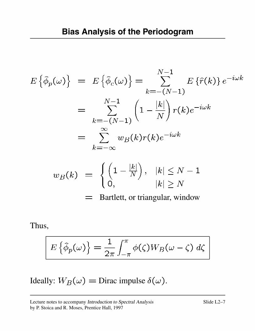
Bias Analysis of the Periodogram
En�p(!)
o= E
n�c(!)
o=
N�1Xk=�(N�1)
E fr(k)g e�i!k
=N�1X
k=�(N�1)
1�jkj
N
!r(k)e�i!k
=1X
k=�1
wB(k)r(k)e�i!k
wB(k) =
8<:�1�
jkjN
�; jkj � N � 1
0; jkj � N
= Bartlett, or triangular, window
Thus,
En�p(!)
o=
1
2�
Z ���
�(�)WB(! � �) d�
Ideally: WB(!) = Dirac impulse �(!).
Lecture notes to accompany Introduction to Spectral Analysis Slide L2–7by P. Stoica and R. Moses, Prentice Hall, 1997
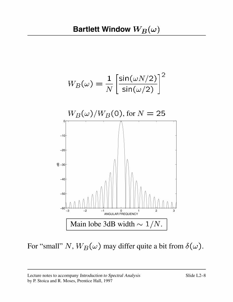
Bartlett Window WB(!)
WB(!) =1
N
"sin(!N=2)
sin(!=2)
#2
WB(!)=WB(0), for N = 25
−3 −2 −1 0 1 2 3−60
−50
−40
−30
−20
−10
0
dB
ANGULAR FREQUENCY
Main lobe 3dB width� 1=N .
For “small” N , WB(!) may differ quite a bit from �(!).
Lecture notes to accompany Introduction to Spectral Analysis Slide L2–8by P. Stoica and R. Moses, Prentice Hall, 1997
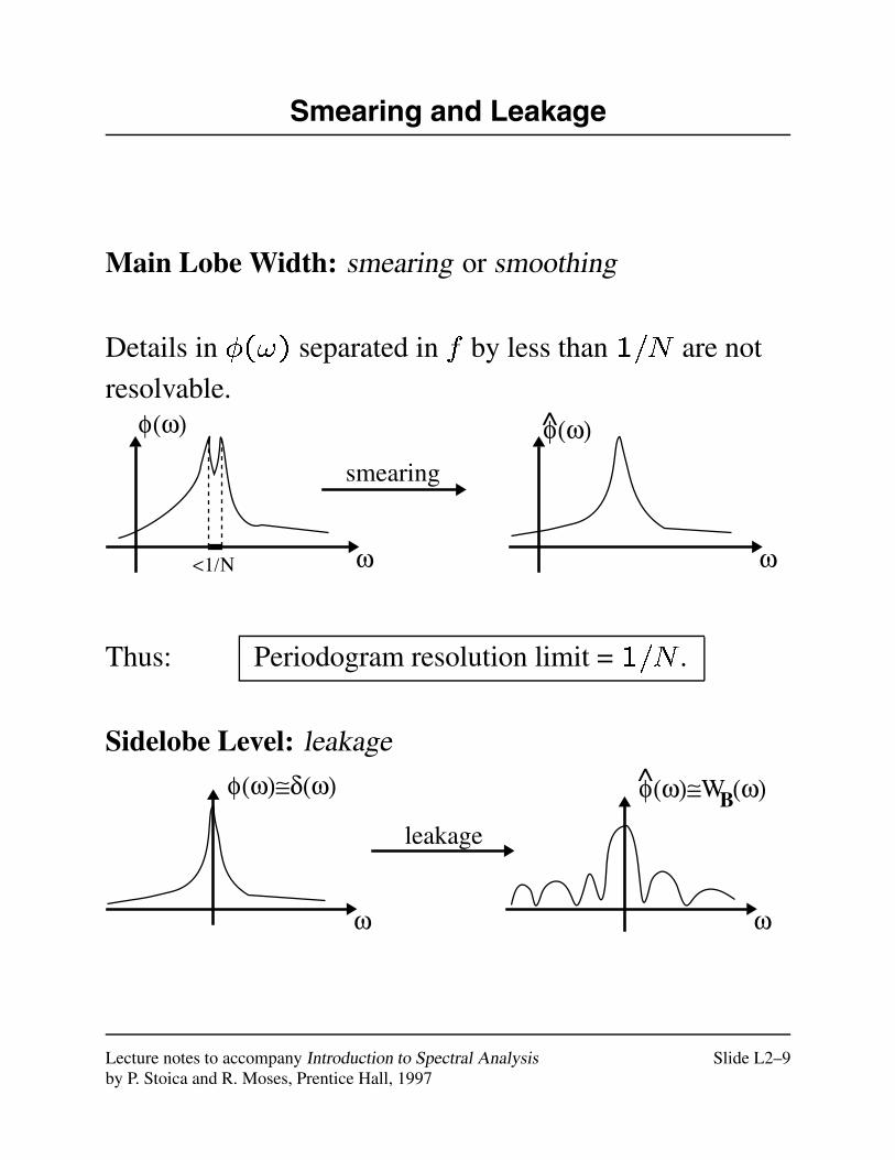
Smearing and Leakage
Main Lobe Width: smearing or smoothing
Details in �(!) separated in f by less than 1=N are not
resolvable.φ(ω)
ω<1/Ν ω
φ(ω)^smearing
Thus: Periodogram resolution limit = 1=N .
Sidelobe Level: leakage
φ(ω)≅δ(ω)
ω ω
φ(ω)≅W (ω)^
leakage
B
Lecture notes to accompany Introduction to Spectral Analysis Slide L2–9by P. Stoica and R. Moses, Prentice Hall, 1997
Periodogram Bias Properties
Summary of Periodogram Bias Properties:
� For “small” N , severe bias
� As N !1, WB(!)! �(!),
so �(!) is asymptotically unbiased.
Lecture notes to accompany Introduction to Spectral Analysis Slide L2–10by P. Stoica and R. Moses, Prentice Hall, 1997

Periodogram Variance
As N !1
Enh�p(!1)� �(!1)
i h�p(!2)� �(!2)
io=
(�2(!1); !1 = !20; !1 6= !2
� Inconsistent estimate
� Erratic behavior
ω
φ(ω)^
1 st. dev = φ(ω) too +-
asymptotic mean = φ(ω)
φ(ω)^
Resolvability properties depend on both bias and variance.
Lecture notes to accompany Introduction to Spectral Analysis Slide L2–11by P. Stoica and R. Moses, Prentice Hall, 1997

Discrete Fourier Transform (DFT)
Finite DTFT: YN(!) =NXt=1
y(t)e�i!t
Let ! = 2�N k and W = e�i
2�N .
Then YN(2�N k) is the Discrete Fourier Transform (DFT):
Y (k) =NXt=1
y(t)W tk; k = 0; : : : ; N � 1
Direct computation of fY (k)gN�1k=0 from fy(t)gNt=1:
O(N2) flops
Lecture notes to accompany Introduction to Spectral Analysis Slide L2–12by P. Stoica and R. Moses, Prentice Hall, 1997
Radix–2 Fast Fourier Transform (FFT)
Assume: N = 2m
Y (k) =
N=2Xt=1
y(t)W tk+NX
t=N=2+1
y(t)W tk
=
N=2Xt=1
[y(t) + y(t+N=2)WNk2 ]W tk
with WNk2 =
�+1; for even k
�1; for odd k
Let ~N = N=2 and ~W =W2 = e�i2�= ~N .
For k = 0;2;4; : : : ; N � 24= 2p:
Y (2p) =
~NXt=1
[y(t) + y(t+ ~N)] ~W tp
For k = 1;3;5; : : : ; N � 1 = 2p+1:
Y (2p+1) =
~NXt=1
f[y(t)� y(t+ ~N)]W tg ~W tp
Each is a ~N = N=2-point DFT computation.
Lecture notes to accompany Introduction to Spectral Analysis Slide L2–13by P. Stoica and R. Moses, Prentice Hall, 1997
FFT Computation Count
Let ck = number of flops for N = 2k point FFT.
Then
ck =2k
2+ 2ck�1
) ck =k2k
2
Thus,
ck =12N log2N
Lecture notes to accompany Introduction to Spectral Analysis Slide L2–14by P. Stoica and R. Moses, Prentice Hall, 1997

Zero Padding
Append the given data by zeros prior to computing DFT
(or FFT):
fy(1); : : : ; y(N);0; : : : 0| {z }N
g
Goals:
� Apply a radix-2 FFT (so N = power of 2)
� Finer sampling of �(!):
�2�
Nk
�N�1k=0
!
�2�
Nk
�N�1k=0
ω
φ(ω)^continuous curve
sampled, N=8
Lecture notes to accompany Introduction to Spectral Analysis Slide L2–15by P. Stoica and R. Moses, Prentice Hall, 1997
Improved Periodogram-Based
Methods
Lecture 3
Lecture notes to accompany Introduction to Spectral Analysis Slide L3–1by P. Stoica and R. Moses, Prentice Hall, 1997
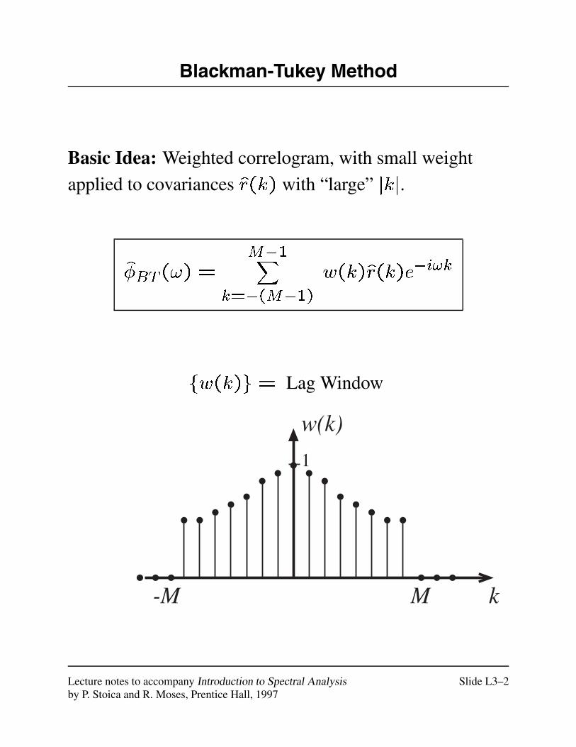
Blackman-Tukey Method
Basic Idea: Weighted correlogram, with small weight
applied to covariances r(k) with “large” jkj.
�BT (!) =M�1X
k=�(M�1)
w(k)r(k)e�i!k
fw(k)g = Lag Window
1
-M M
w(k)
k
Lecture notes to accompany Introduction to Spectral Analysis Slide L3–2by P. Stoica and R. Moses, Prentice Hall, 1997
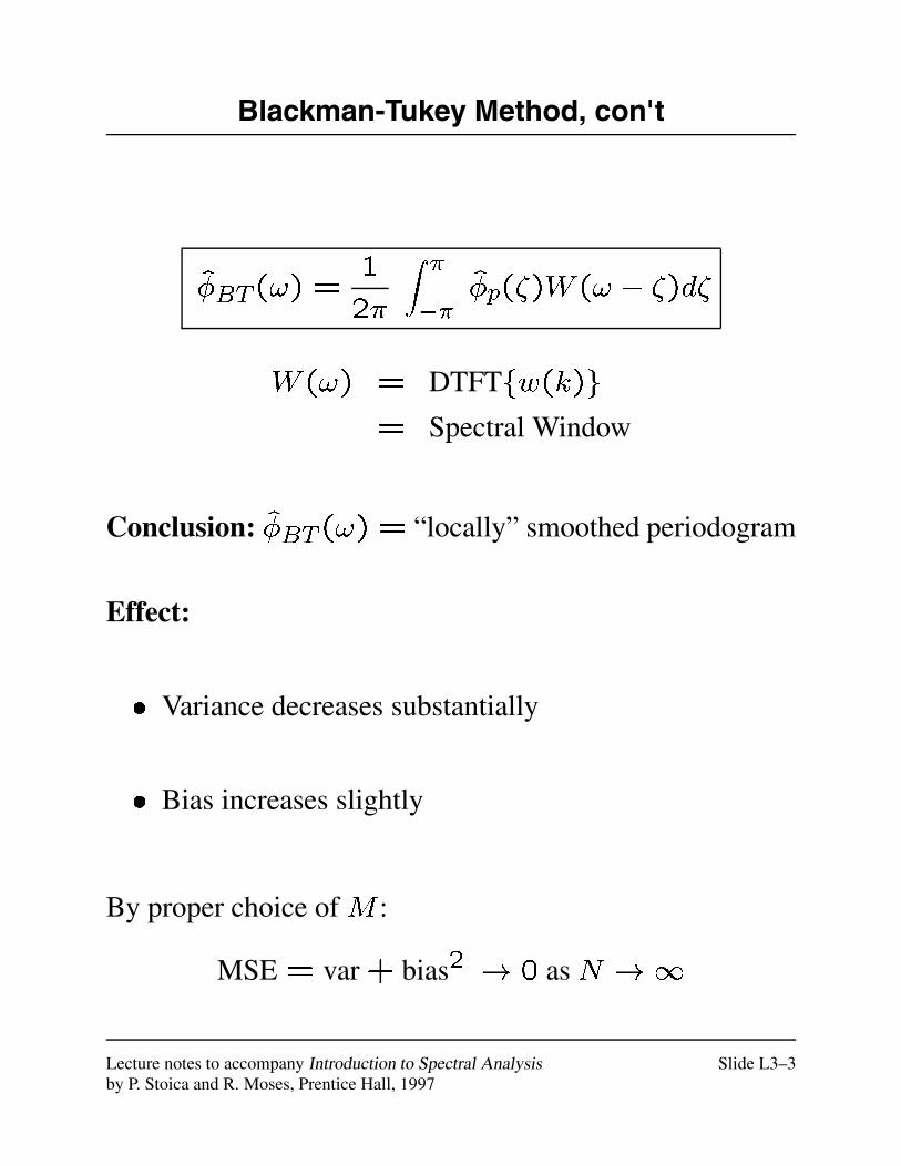
Blackman-Tukey Method, con't
�BT (!) =1
2�
Z ���
�p(�)W(! � �)d�
W(!) = DTFTfw(k)g
= Spectral Window
Conclusion: �BT (!) = “locally” smoothed periodogram
Effect:
� Variance decreases substantially
� Bias increases slightly
By proper choice of M :
MSE = var + bias2 ! 0 as N !1
Lecture notes to accompany Introduction to Spectral Analysis Slide L3–3by P. Stoica and R. Moses, Prentice Hall, 1997
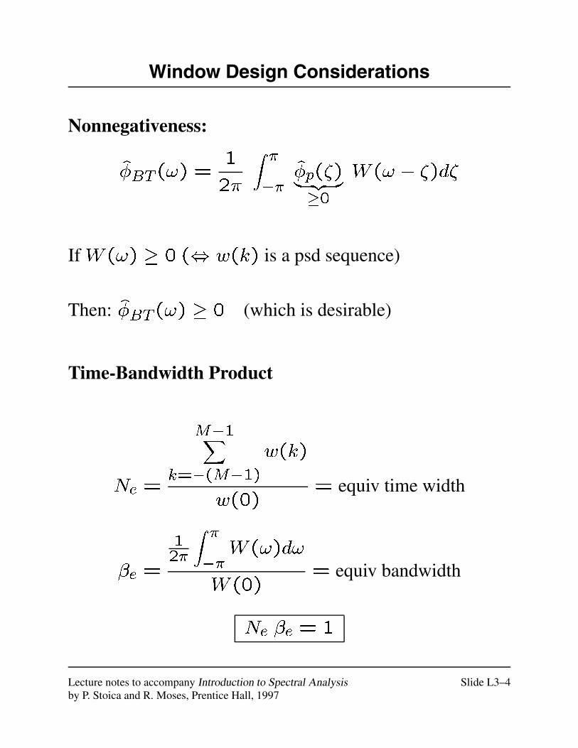
Window Design Considerations
Nonnegativeness:
�BT (!) =1
2�
Z ���
�p(�)| {z }�0
W(! � �)d�
If W(!) � 0 (, w(k) is a psd sequence)
Then: �BT (!) � 0 (which is desirable)
Time-Bandwidth Product
Ne =
M�1Xk=�(M�1)
w(k)
w(0)= equiv time width
�e =
12�
Z ���
W(!)d!
W(0)= equiv bandwidth
Ne �e = 1
Lecture notes to accompany Introduction to Spectral Analysis Slide L3–4by P. Stoica and R. Moses, Prentice Hall, 1997
Window Design, con't
� �e = 1=Ne = 0(1=M)
is the BT resolution threshold.
� As M increases, bias decreases and variance
increases.
) Choose M as a tradeoff between variance and
bias.
� Once M is given, Ne (and hence �e) is essentially
fixed.
) Choose window shape to compromise between
smearing (main lobe width) and leakage (sidelobe
level).
The energy in the main lobe and in the sidelobes
cannot be reduced simultaneously, once M is given.
Lecture notes to accompany Introduction to Spectral Analysis Slide L3–5by P. Stoica and R. Moses, Prentice Hall, 1997
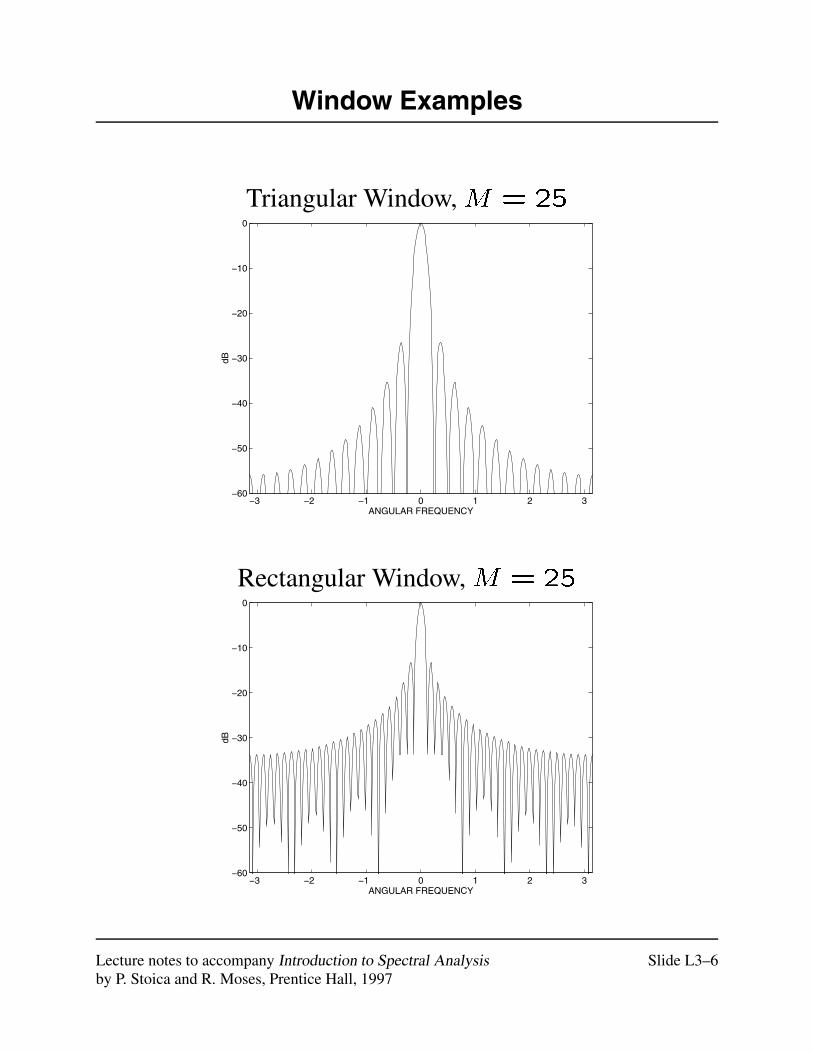
Window Examples
Triangular Window, M = 25
−3 −2 −1 0 1 2 3−60
−50
−40
−30
−20
−10
0dB
ANGULAR FREQUENCY
Rectangular Window, M = 25
−3 −2 −1 0 1 2 3−60
−50
−40
−30
−20
−10
0
dB
ANGULAR FREQUENCY
Lecture notes to accompany Introduction to Spectral Analysis Slide L3–6by P. Stoica and R. Moses, Prentice Hall, 1997
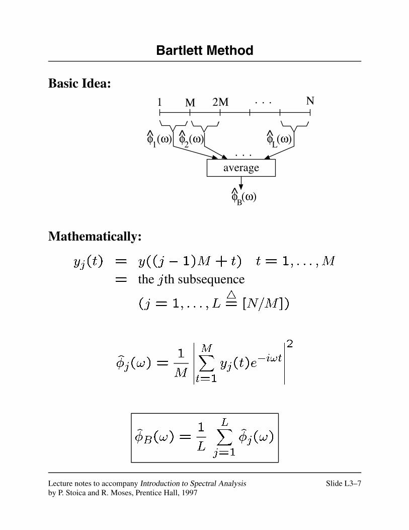
Bartlett Method
Basic Idea:1 Μ 2Μ Ν. . .
average. . .
φ (ω)1
φ (ω)2
φ (ω)L
φ (ω)B
Mathematically:
yj(t) = y((j � 1)M + t) t = 1; : : : ;M
= the jth subsequence
(j = 1; : : : ; L4= [N=M ])
�j(!) =1
M
������MXt=1
yj(t)e�i!t
������2
�B(!) =1
L
LXj=1
�j(!)
Lecture notes to accompany Introduction to Spectral Analysis Slide L3–7by P. Stoica and R. Moses, Prentice Hall, 1997
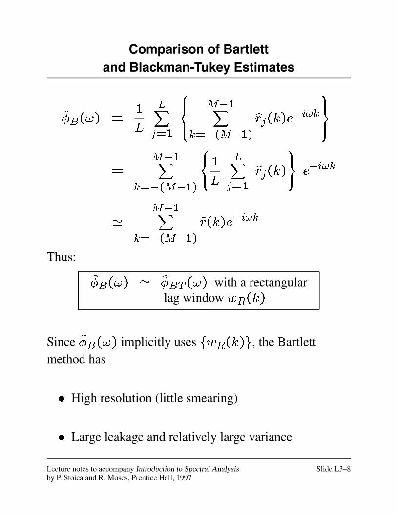
Comparison of Bartlettand Blackman-Tukey Estimates
�B(!) =1
L
LXj=1
8><>:
M�1Xk=�(M�1)
rj(k)e�i!k
9>=>;
=M�1X
k=�(M�1)
8<:1L
LXj=1
rj(k)
9=; e�i!k
'M�1X
k=�(M�1)
r(k)e�i!k
Thus:
�B(!) ' �BT (!) with a rectangularlag window wR(k)
Since �B(!) implicitly uses fwR(k)g, the Bartlettmethod has
� High resolution (little smearing)
� Large leakage and relatively large variance
Lecture notes to accompany Introduction to Spectral Analysis Slide L3–8by P. Stoica and R. Moses, Prentice Hall, 1997
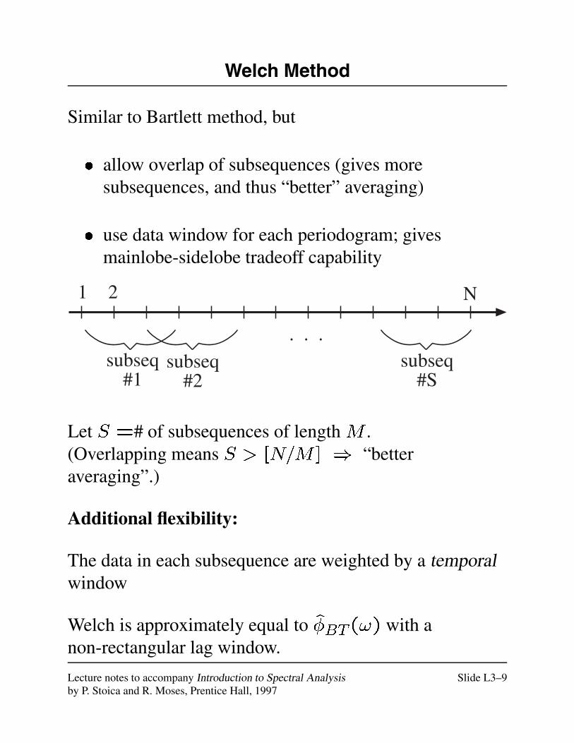
Welch Method
Similar to Bartlett method, but
� allow overlap of subsequences (gives moresubsequences, and thus “better” averaging)
� use data window for each periodogram; givesmainlobe-sidelobe tradeoff capability
1 2 N
subseq#1
. . .
subseq#2
subseq#S
Let S =# of subsequences of length M .(Overlapping means S > [N=M ] ) “betteraveraging”.)
Additional flexibility:
The data in each subsequence are weighted by a temporalwindow
Welch is approximately equal to �BT (!) with anon-rectangular lag window.
Lecture notes to accompany Introduction to Spectral Analysis Slide L3–9by P. Stoica and R. Moses, Prentice Hall, 1997

Daniell Method
By a previous result, for N � 1,
f�p(!j)g are (nearly) uncorrelated random variables for
�!j =
2�
Nj
�N�1j=0
Idea: “Local averaging” of (2J +1) samples in the
frequency domain should reduce the variance by about
(2J +1).
�D(!k) =1
2J +1
k+JXj=k�J
�p (!j)
Lecture notes to accompany Introduction to Spectral Analysis Slide L3–10by P. Stoica and R. Moses, Prentice Hall, 1997
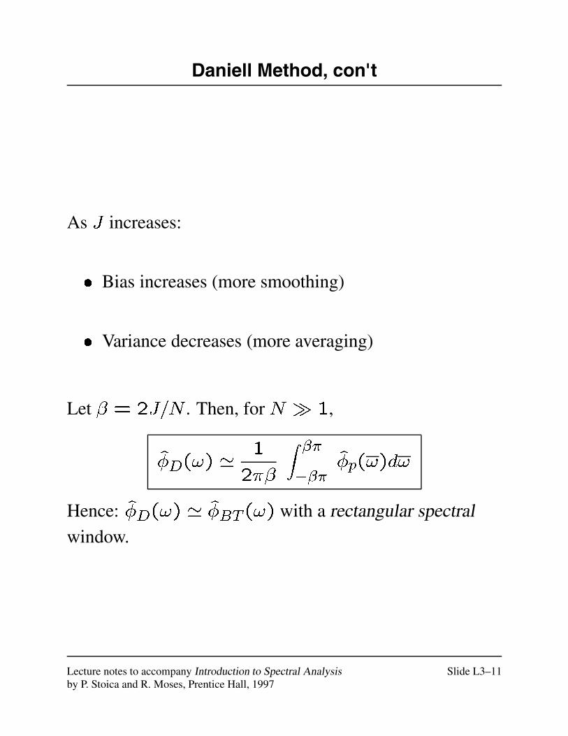
Daniell Method, con't
As J increases:
� Bias increases (more smoothing)
� Variance decreases (more averaging)
Let � = 2J=N . Then, for N � 1,
�D(!) '1
2��
Z �����
�p(!)d!
Hence: �D(!) ' �BT (!) with a rectangular spectralwindow.
Lecture notes to accompany Introduction to Spectral Analysis Slide L3–11by P. Stoica and R. Moses, Prentice Hall, 1997
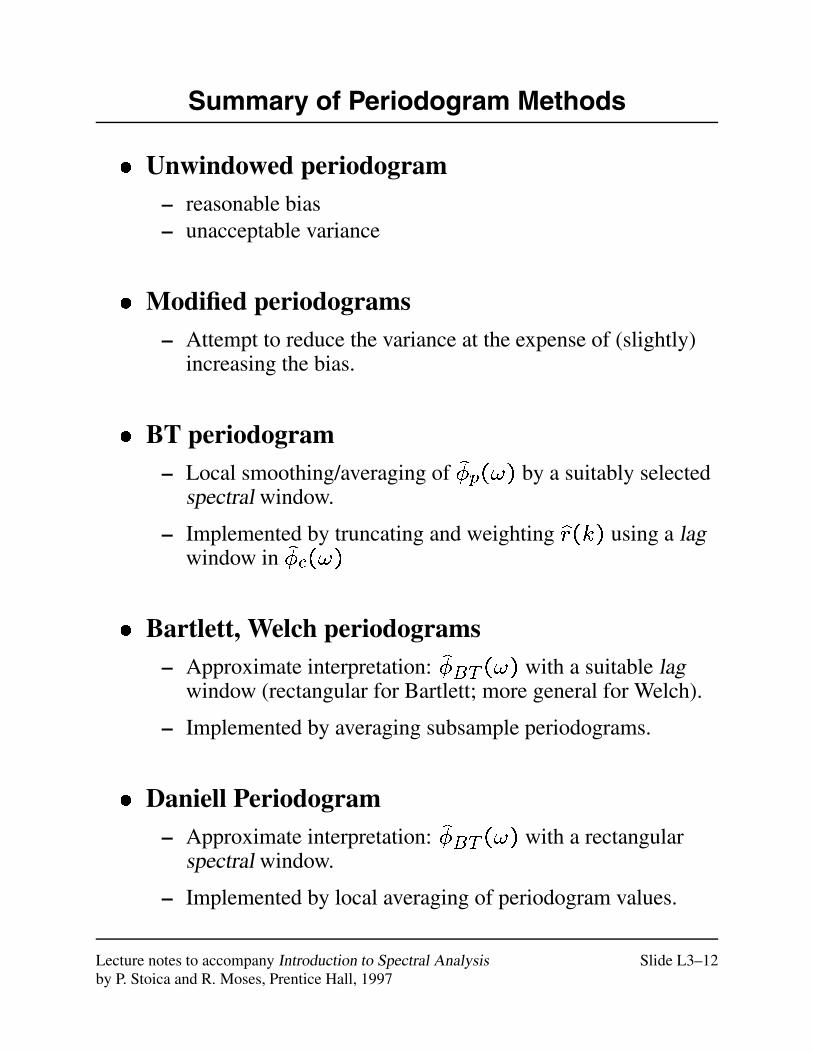
Summary of Periodogram Methods
� Unwindowed periodogram– reasonable bias– unacceptable variance
� Modified periodograms– Attempt to reduce the variance at the expense of (slightly)
increasing the bias.
� BT periodogram– Local smoothing/averaging of �p(!) by a suitably selected
spectral window.
– Implemented by truncating and weighting r(k) using a lagwindow in �c(!)
� Bartlett, Welch periodograms– Approximate interpretation: �BT (!) with a suitable lag
window (rectangular for Bartlett; more general for Welch).
– Implemented by averaging subsample periodograms.
� Daniell Periodogram– Approximate interpretation: �BT (!) with a rectangular
spectral window.
– Implemented by local averaging of periodogram values.
Lecture notes to accompany Introduction to Spectral Analysis Slide L3–12by P. Stoica and R. Moses, Prentice Hall, 1997
Parametric Methods
for
Rational Spectra
Lecture 4
Lecture notes to accompany Introduction to Spectral Analysis Slide L4–1by P. Stoica and R. Moses, Prentice Hall, 1997
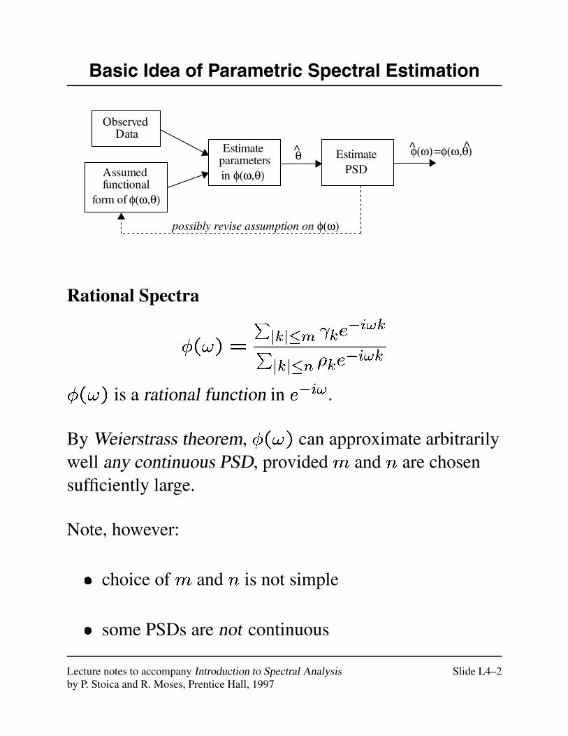
Basic Idea of Parametric Spectral Estimation
Observed Data
Assumed functional
form of φ(ω,θ)
Estimate parametersin φ(ω,θ)
Estimate PSD
φ(ω) =φ(ω,θ)^ ^θ
possibly revise assumption on φ(ω)
Rational Spectra
�(!) =
Pjkj�m ke
�i!kPjkj�n �ke
�i!k
�(!) is a rational function in e�i!.
By Weierstrass theorem, �(!) can approximate arbitrarilywell any continuous PSD, provided m and n are chosensufficiently large.
Note, however:
� choice of m and n is not simple
� some PSDs are not continuous
Lecture notes to accompany Introduction to Spectral Analysis Slide L4–2by P. Stoica and R. Moses, Prentice Hall, 1997
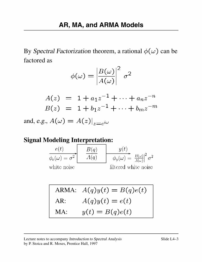
AR, MA, and ARMA Models
By Spectral Factorization theorem, a rational �(!) can be
factored as
�(!) =
�����B(!)A(!)
�����2
�2
A(z) = 1+ a1z�1+ � � �+ anz
�n
B(z) = 1+ b1z�1+ � � �+ bmz
�m
and, e.g., A(!) = A(z)jz=ei!
Signal Modeling Interpretation:e(t)
�e(!) = �2
white noise
y(t)
�y(!) =����
B(!)A(!)
����
2�2
B(q)
A(q)
�ltered white noise
--
ARMA: A(q)y(t) = B(q)e(t)
AR: A(q)y(t) = e(t)
MA: y(t) = B(q)e(t)
Lecture notes to accompany Introduction to Spectral Analysis Slide L4–3by P. Stoica and R. Moses, Prentice Hall, 1997
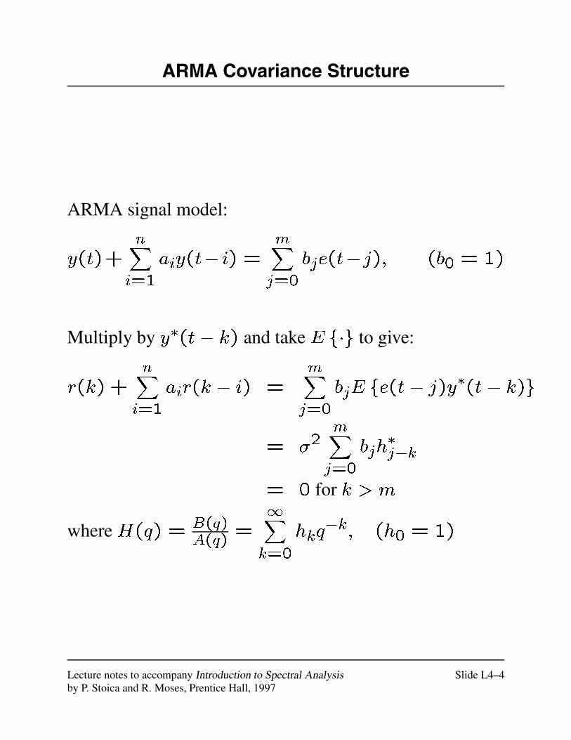
ARMA Covariance Structure
ARMA signal model:
y(t)+nXi=1
aiy(t� i) =mXj=0
bje(t�j); (b0 = 1)
Multiply by y�(t� k) and take E f�g to give:
r(k) +nXi=1
air(k � i) =mXj=0
bjE fe(t� j)y�(t� k)g
= �2mXj=0
bjh�j�k
= 0 for k > m
where H(q) = B(q)A(q)
=1Xk=0
hkq�k; (h0 = 1)
Lecture notes to accompany Introduction to Spectral Analysis Slide L4–4by P. Stoica and R. Moses, Prentice Hall, 1997
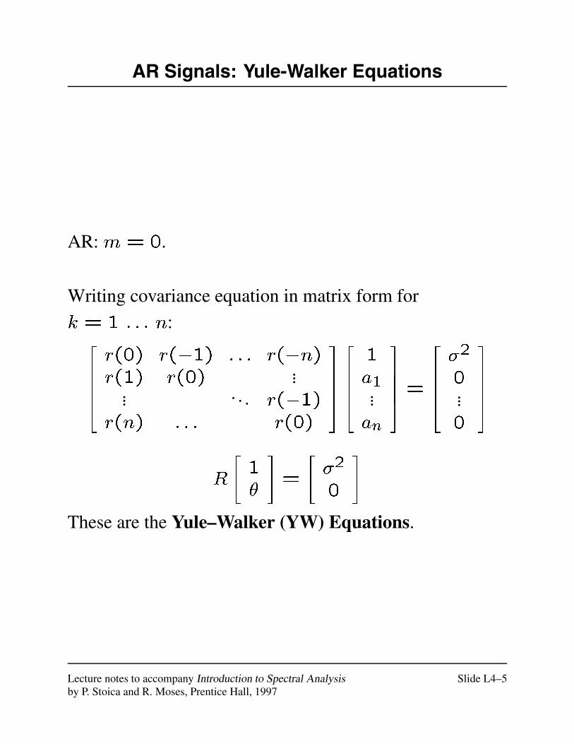
AR Signals: Yule-Walker Equations
AR: m = 0.
Writing covariance equation in matrix form for
k = 1 : : : n:26664r(0) r(�1) : : : r(�n)r(1) r(0) ...
... . . . r(�1)r(n) : : : r(0)
3777526664
1a1...an
37775=
26664�2
0...0
37775
R
"1�
#=
"�2
0
#
These are the Yule–Walker (YW) Equations.
Lecture notes to accompany Introduction to Spectral Analysis Slide L4–5by P. Stoica and R. Moses, Prentice Hall, 1997

AR Spectral Estimation: YW Method
Yule-Walker Method:
Replace r(k) by r(k) and solve for faig and �2:26664r(0) r(�1) : : : r(�n)r(1) r(0) ...
... . . . r(�1)r(n) : : : r(0)
3777526664
1a1...an
37775=
26664�2
0...0
37775
Then the PSD estimate is
�(!) =�2
jA(!)j2
Lecture notes to accompany Introduction to Spectral Analysis Slide L4–6by P. Stoica and R. Moses, Prentice Hall, 1997
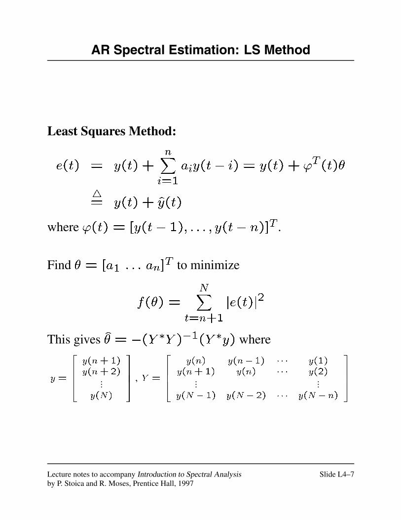
AR Spectral Estimation: LS Method
Least Squares Method:
e(t) = y(t) +nXi=1
aiy(t� i) = y(t) + 'T (t)�
4= y(t) + y(t)
where '(t) = [y(t� 1); : : : ; y(t� n)]T .
Find � = [a1 : : : an]T to minimize
f(�) =NX
t=n+1
je(t)j2
This gives � = �(Y �Y )�1(Y �y) where
y =
264
y(n+1)y(n+2)
...y(N)
375 ; Y =
264
y(n) y(n� 1) � � � y(1)y(n+1) y(n) � � � y(2)
......
y(N � 1) y(N � 2) � � � y(N � n)
375
Lecture notes to accompany Introduction to Spectral Analysis Slide L4–7by P. Stoica and R. Moses, Prentice Hall, 1997
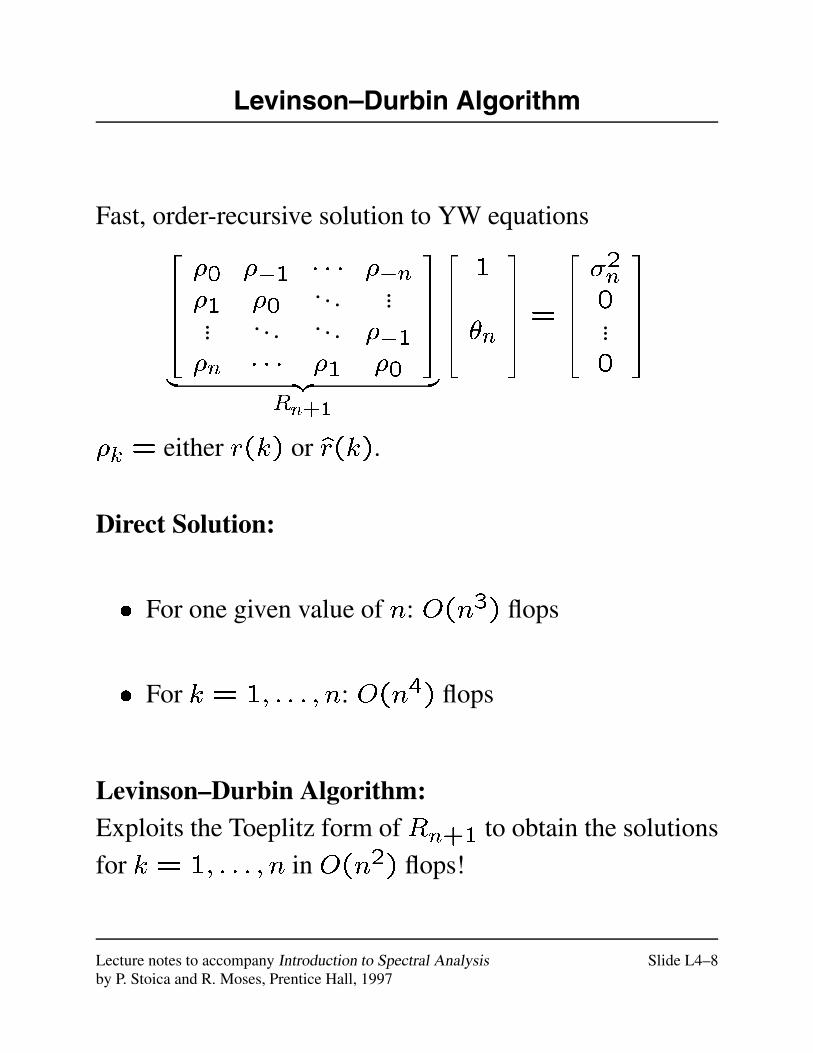
Levinson–Durbin Algorithm
Fast, order-recursive solution to YW equations26664�0 ��1 � � � ��n�1 �0
. . . ...... . . . . . . ��1�n � � � �1 �0
37775
| {z }Rn+1
266641
�n
37775=
26664�2n0...0
37775
�k = either r(k) or r(k).
Direct Solution:
� For one given value of n: O(n3) flops
� For k = 1; : : : ; n: O(n4) flops
Levinson–Durbin Algorithm:Exploits the Toeplitz form of Rn+1 to obtain the solutions
for k = 1; : : : ; n in O(n2) flops!
Lecture notes to accompany Introduction to Spectral Analysis Slide L4–8by P. Stoica and R. Moses, Prentice Hall, 1997
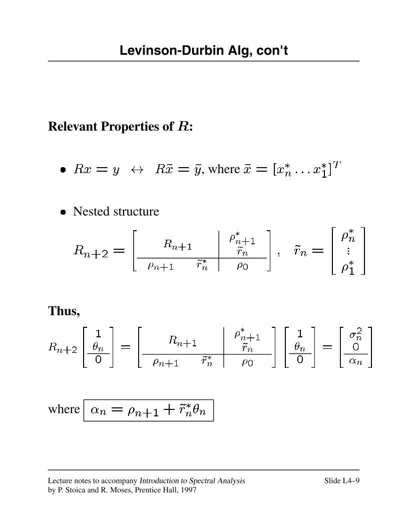
Levinson-Durbin Alg, con't
Relevant Properties ofR:
� Rx = y $ R~x = ~y, where ~x = [x�n : : : x�1]T
� Nested structure
Rn+2 =
24 Rn+1
��n+1~rn
�n+1 ~r�n �0
35 ; ~rn =
264 �
�n...��1
375
Thus,
Rn+2
24 1�n0
35=
24 Rn+1
��n+1~rn
�n+1 ~r�n �0
3524 1�n0
35=
24 �2n
0�n
35
where �n = �n+1+~r�n�n
Lecture notes to accompany Introduction to Spectral Analysis Slide L4–9by P. Stoica and R. Moses, Prentice Hall, 1997
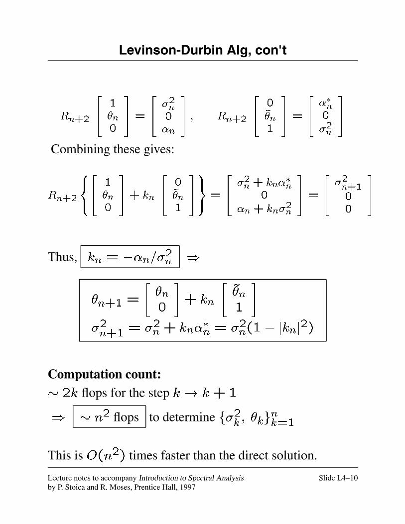
Levinson-Durbin Alg, con't
Rn+2
24 1�n0
35 =
24 �2n
0�n
35 ; Rn+2
24 0~�n1
35=
24 ��n
0
�2n
35
Combining these gives:
Rn+2
8<:24 1�n0
35+ kn
24 0~�n1
359=;=
24 �2n + kn��n
0
�n+ kn�2n
35=
24 �2
n+100
35
Thus, kn = ��n=�2n )
�n+1 =
"�n0
#+ kn
"~�n1
#
�2n+1 = �2n+ kn��n = �2n(1� jknj2)
Computation count:� 2k flops for the step k ! k+1
) � n2 flops to determine f�2k ; �kgnk=1
This is O(n2) times faster than the direct solution.
Lecture notes to accompany Introduction to Spectral Analysis Slide L4–10by P. Stoica and R. Moses, Prentice Hall, 1997
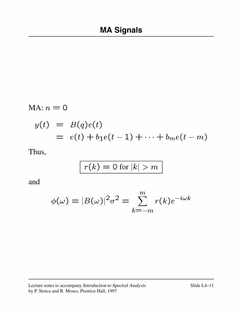
MA Signals
MA: n= 0
y(t) = B(q)e(t)
= e(t) + b1e(t� 1) + � � �+ bme(t�m)
Thus,
r(k) = 0 for jkj > m
and
�(!) = jB(!)j2�2 =mX
k=�m
r(k)e�i!k
Lecture notes to accompany Introduction to Spectral Analysis Slide L4–11by P. Stoica and R. Moses, Prentice Hall, 1997
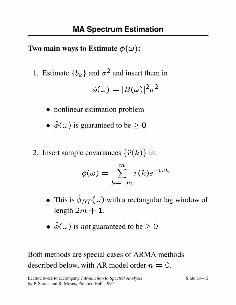
MA Spectrum Estimation
Two main ways to Estimate �(!):
1. Estimate fbkg and �2 and insert them in
�(!) = jB(!)j2�2
� nonlinear estimation problem
� �(!) is guaranteed to be� 0
2. Insert sample covariances fr(k)g in:
�(!) =mX
k=�m
r(k)e�i!k
� This is �BT (!) with a rectangular lag window of
length 2m+1.
� �(!) is not guaranteed to be� 0
Both methods are special cases of ARMA methods
described below, with AR model order n = 0.
Lecture notes to accompany Introduction to Spectral Analysis Slide L4–12by P. Stoica and R. Moses, Prentice Hall, 1997
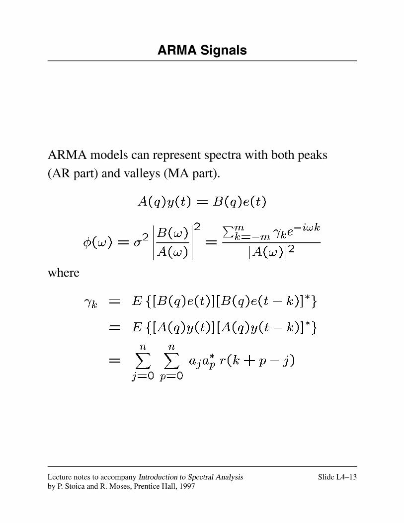
ARMA Signals
ARMA models can represent spectra with both peaks
(AR part) and valleys (MA part).
A(q)y(t) = B(q)e(t)
�(!) = �2�����B(!)A(!)
�����2
=
Pmk=�m ke
�i!k
jA(!)j2
where
k = E f[B(q)e(t)][B(q)e(t � k)]�g
= E f[A(q)y(t)][A(q)y(t � k)]�g
=nX
j=0
nXp=0
aja�p r(k+ p� j)
Lecture notes to accompany Introduction to Spectral Analysis Slide L4–13by P. Stoica and R. Moses, Prentice Hall, 1997
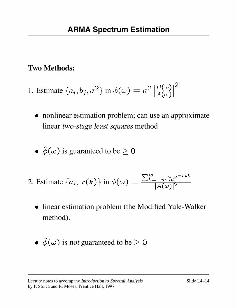
ARMA Spectrum Estimation
Two Methods:
1. Estimate fai; bj; �2g in �(!) = �2���B(!)A(!)
���2
� nonlinear estimation problem; can use an approximate
linear two-stage least squares method
� �(!) is guaranteed to be� 0
2. Estimate fai; r(k)g in �(!) =Pm
k=�m ke�i!k
jA(!)j2
� linear estimation problem (the Modified Yule-Walker
method).
� �(!) is not guaranteed to be� 0
Lecture notes to accompany Introduction to Spectral Analysis Slide L4–14by P. Stoica and R. Moses, Prentice Hall, 1997
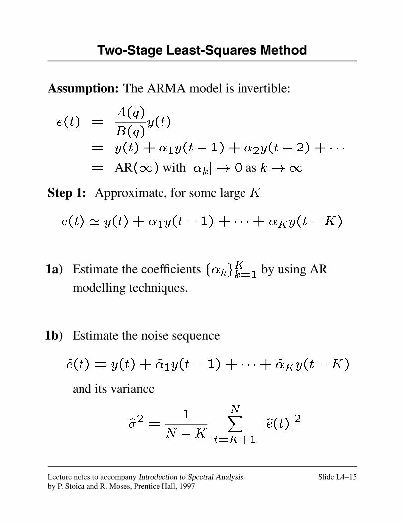
Two-Stage Least-Squares Method
Assumption: The ARMA model is invertible:
e(t) =A(q)
B(q)y(t)
= y(t) + �1y(t� 1) + �2y(t� 2) + � � �
= AR(1) with j�kj ! 0 as k !1
Step 1: Approximate, for some large K
e(t) ' y(t) + �1y(t� 1) + � � �+ �Ky(t�K)
1a) Estimate the coefficients f�kgKk=1 by using AR
modelling techniques.
1b) Estimate the noise sequence
e(t) = y(t) + �1y(t� 1) + � � �+ �Ky(t�K)
and its variance
�2 =1
N �K
NXt=K+1
je(t)j2
Lecture notes to accompany Introduction to Spectral Analysis Slide L4–15by P. Stoica and R. Moses, Prentice Hall, 1997
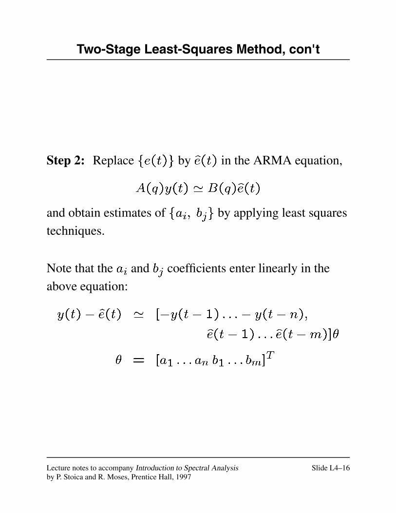
Two-Stage Least-Squares Method, con't
Step 2: Replace fe(t)g by e(t) in the ARMA equation,
A(q)y(t) ' B(q)e(t)
and obtain estimates of fai; bjg by applying least squares
techniques.
Note that the ai and bj coefficients enter linearly in the
above equation:
y(t)� e(t) ' [�y(t� 1) : : :� y(t� n);
e(t� 1) : : : e(t�m)]�
� = [a1 : : : an b1 : : : bm]T
Lecture notes to accompany Introduction to Spectral Analysis Slide L4–16by P. Stoica and R. Moses, Prentice Hall, 1997
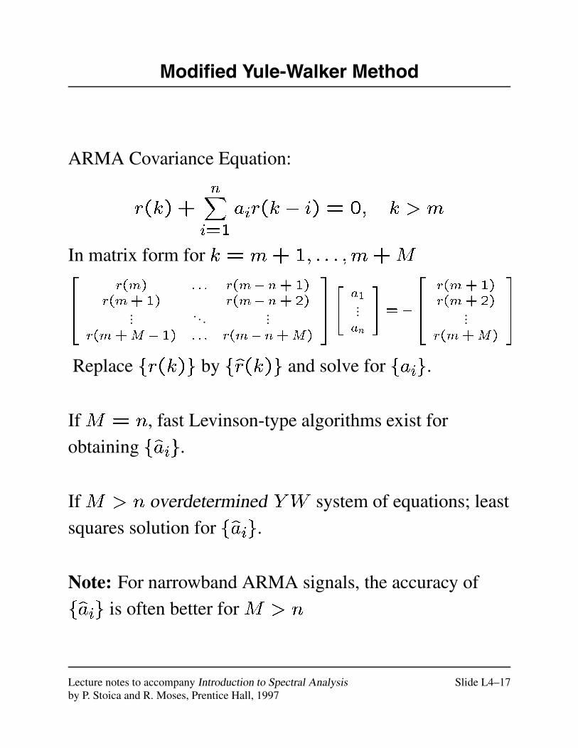
Modified Yule-Walker Method
ARMA Covariance Equation:
r(k) +nXi=1
air(k � i) = 0; k > m
In matrix form for k = m+1; : : : ;m+M264
r(m) : : : r(m� n+1)r(m+1) r(m� n+2)
... . . . ...r(m+M � 1) : : : r(m� n+M)
375"
a1...an
#= �
264
r(m+1)r(m+2)
...r(m+M)
375
Replace fr(k)g by fr(k)g and solve for faig.
If M = n, fast Levinson-type algorithms exist for
obtaining faig.
If M > n overdetermined YW system of equations; least
squares solution for faig.
Note: For narrowband ARMA signals, the accuracy of
faig is often better for M > n
Lecture notes to accompany Introduction to Spectral Analysis Slide L4–17by P. Stoica and R. Moses, Prentice Hall, 1997

Su
mm
ary
of
Par
amet
ric
Met
ho
ds
for
Rat
ion
alS
pec
tra
Com
puta
tiona
lG
uara
ntee
Met
hod
Bur
den
Acc
urac
y
^ �(!)�
0
?U
sefo
rA
R:Y
Wor
LS
low
med
ium
Yes
Spec
tra
with
(nar
row
)pe
aks
but
nova
lley
MA
:BT
low
low
-med
ium
No
Bro
adba
ndsp
ectr
apo
ssib
lyw
ithva
lleys
butn
ope
aks
AR
MA
:MY
Wlo
w-m
ediu
mm
ediu
mN
oSp
ectr
aw
ithbo
thpe
aks
and
(not
too
deep
)va
lleys
AR
MA
:2-S
tage
LS
med
ium
-hig
hm
ediu
m-h
igh
Yes
As
abov
e
Lec
ture
note
sto
acco
mpa
nyIn
trod
uctio
nto
Spec
tral
Ana
lysi
sSl
ide
L4–
18by
P.St
oica
and
R.M
oses
,Pre
ntic
eH
all,
1997
Parametric Methods
for
Line Spectra — Part 1
Lecture 5
Lecture notes to accompany Introduction to Spectral Analysis Slide L5–1by P. Stoica and R. Moses, Prentice Hall, 1997
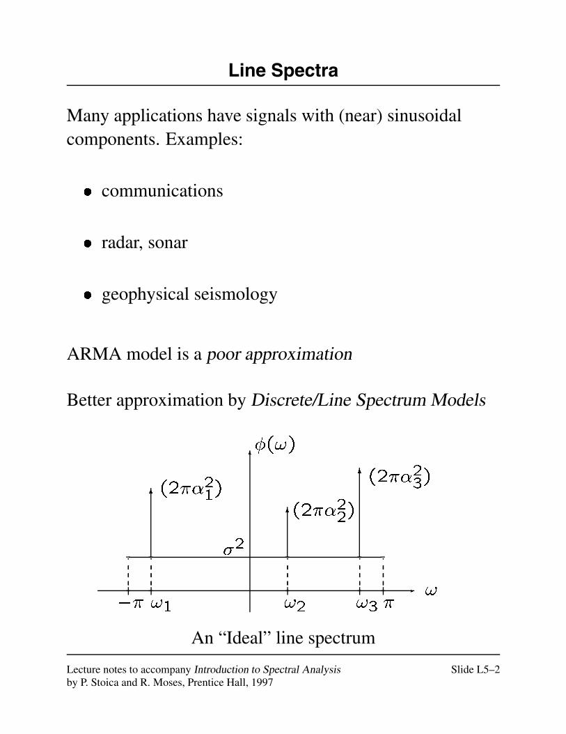
Line Spectra
Many applications have signals with (near) sinusoidalcomponents. Examples:
� communications
� radar, sonar
� geophysical seismology
ARMA model is a poor approximation
Better approximation by Discrete/Line Spectrum Models
-
6
6
6
6
�2
�� �!1 !2 !3
(2��21)(2��22)
(2��23)
!
�(!)
An “Ideal” line spectrum
Lecture notes to accompany Introduction to Spectral Analysis Slide L5–2by P. Stoica and R. Moses, Prentice Hall, 1997
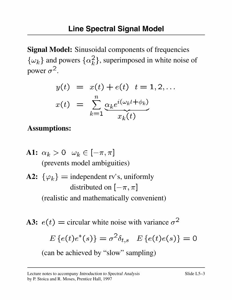
Line Spectral Signal Model
Signal Model: Sinusoidal components of frequencies
f!kg and powers f�2kg, superimposed in white noise of
power �2.
y(t) = x(t) + e(t) t = 1;2; : : :
x(t) =nX
k=1
�kei(!kt+�k)| {z }xk(t)
Assumptions:
A1: �k > 0 !k 2 [��; �]
(prevents model ambiguities)
A2: f'kg= independent rv's, uniformly
distributed on [��; �]
(realistic and mathematically convenient)
A3: e(t) = circular white noise with variance �2
E fe(t)e�(s)g = �2�t;s E fe(t)e(s)g = 0
(can be achieved by “slow” sampling)
Lecture notes to accompany Introduction to Spectral Analysis Slide L5–3by P. Stoica and R. Moses, Prentice Hall, 1997
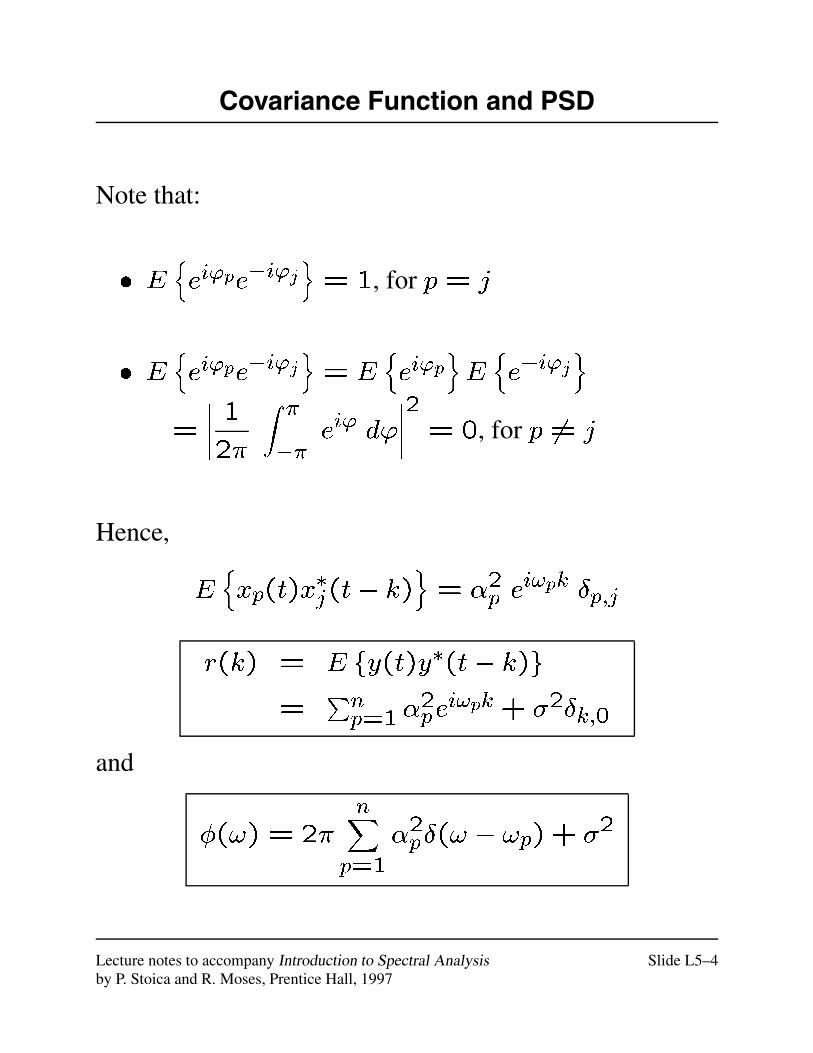
Covariance Function and PSD
Note that:
� Enei'pe�i'j
o= 1, for p = j
� Enei'pe�i'j
o= E
nei'p
oEne�i'j
o=
���� 12�Z ���
ei' d'
����2 = 0, for p 6= j
Hence,
Enxp(t)x
�j(t� k)
o= �2p e
i!pk �p;j
r(k) = E fy(t)y�(t� k)g
=Pnp=1�
2pei!pk+ �2�k;0
and
�(!) = 2�nX
p=1
�2p�(! � !p) + �2
Lecture notes to accompany Introduction to Spectral Analysis Slide L5–4by P. Stoica and R. Moses, Prentice Hall, 1997

Parameter Estimation
Estimate either:
� f!k; �k; 'kgnk=1; �
2 (Signal Model)
� f!k; �2kgnk=1; �
2 (PSD Model)
Major Estimation Problem: f!kg
Once f!kg are determined:
� f�2kg can be obtained by a least squares method from
r(k) =nX
p=1
�2pei!pk + residuals
OR:
� Both f�kg and f'kg can be derived by a leastsquares method from
y(t) =nX
k=1
�kei!kt + residuals
with �k = �kei'k .
Lecture notes to accompany Introduction to Spectral Analysis Slide L5–5by P. Stoica and R. Moses, Prentice Hall, 1997
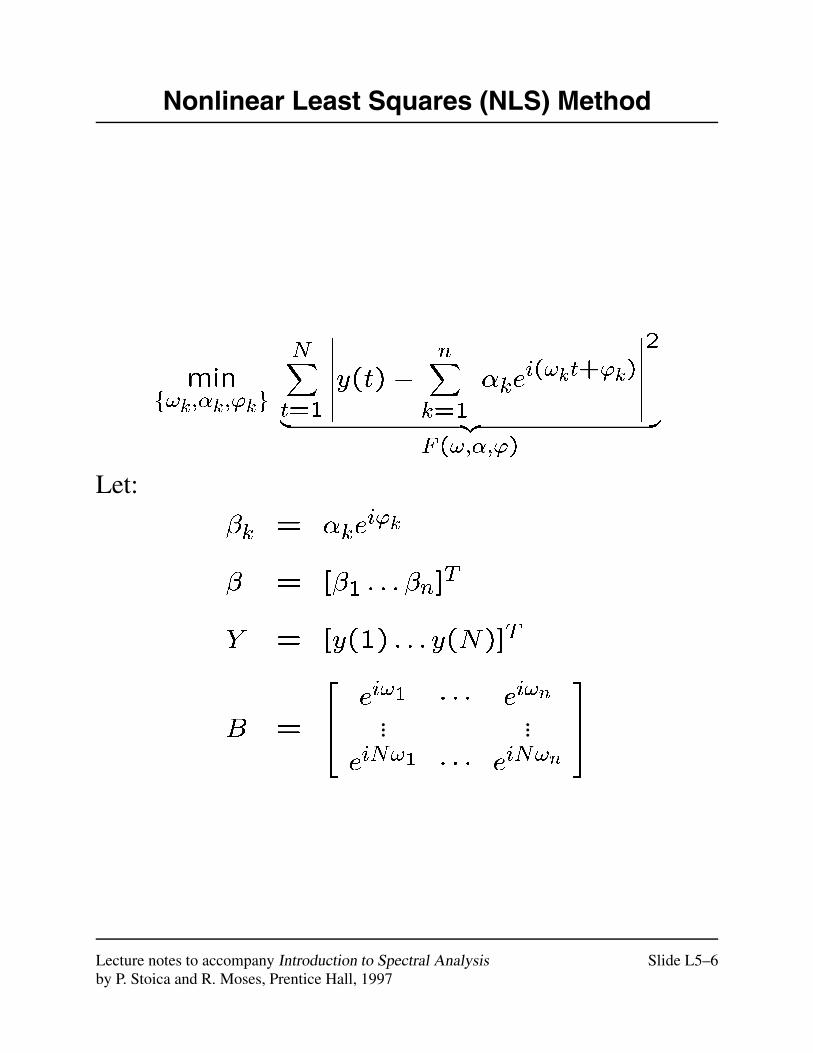
Nonlinear Least Squares (NLS) Method
minf!k;�k;'kg
NXt=1
������y(t)�nX
k=1
�kei(!kt+'k)
������2
| {z }F(!;�;')
Let:
�k = �kei'k
� = [�1 : : : �n]T
Y = [y(1) : : : y(N)]T
B =
264 ei!1 � � � ei!n
... ...eiN!1 � � � eiN!n
375
Lecture notes to accompany Introduction to Spectral Analysis Slide L5–6by P. Stoica and R. Moses, Prentice Hall, 1997
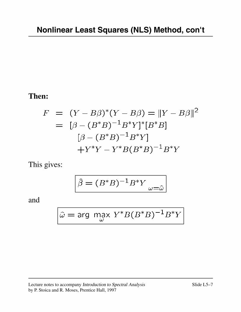
Nonlinear Least Squares (NLS) Method, con't
Then:
F = (Y �B�)�(Y �B�) = kY �B�k2
= [� � (B�B)�1B�Y ]�[B�B]
[� � (B�B)�1B�Y ]
+Y �Y � Y �B(B�B)�1B�Y
This gives:
� = (B�B)�1B�Y���!=!
and
! = arg max!
Y �B(B�B)�1B�Y
Lecture notes to accompany Introduction to Spectral Analysis Slide L5–7by P. Stoica and R. Moses, Prentice Hall, 1997
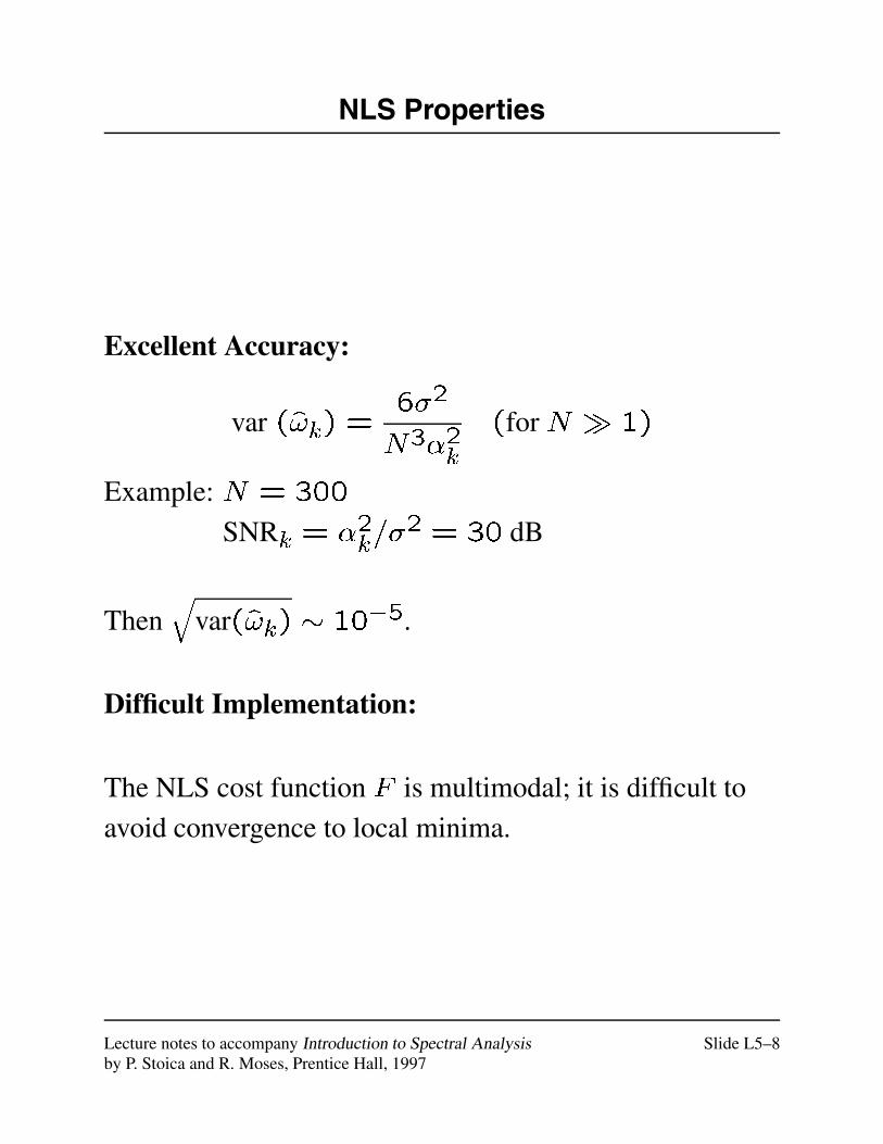
NLS Properties
Excellent Accuracy:
var (!k) =6�2
N3�2k(for N � 1)
Example: N = 300
SNRk = �2k=�2 = 30 dB
Thenq
var(!k) � 10�5.
Difficult Implementation:
The NLS cost function F is multimodal; it is difficult to
avoid convergence to local minima.
Lecture notes to accompany Introduction to Spectral Analysis Slide L5–8by P. Stoica and R. Moses, Prentice Hall, 1997
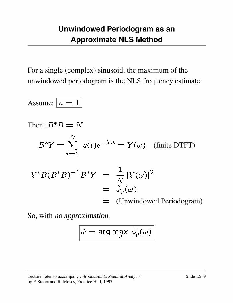
Unwindowed Periodogram as anApproximate NLS Method
For a single (complex) sinusoid, the maximum of the
unwindowed periodogram is the NLS frequency estimate:
Assume: n = 1
Then: B�B = N
B�Y =NXt=1
y(t)e�i!t = Y (!) (finite DTFT)
Y �B(B�B)�1B�Y =1
NjY (!)j2
= �p(!)
= (Unwindowed Periodogram)
So, with no approximation,
! = argmax!
�p(!)
Lecture notes to accompany Introduction to Spectral Analysis Slide L5–9by P. Stoica and R. Moses, Prentice Hall, 1997
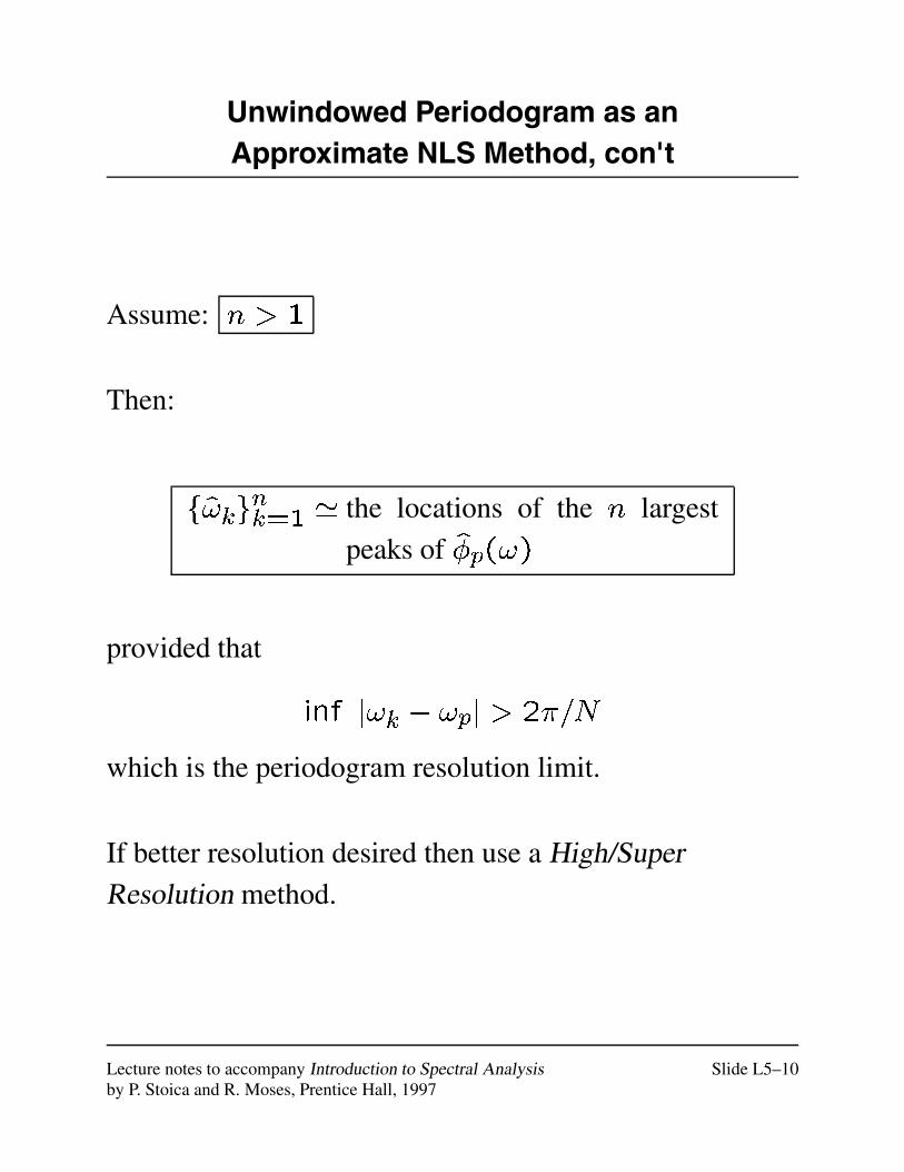
Unwindowed Periodogram as anApproximate NLS Method, con't
Assume: n > 1
Then:
f!kgnk=1 ' the locations of the n largest
peaks of �p(!)
provided that
inf j!k � !pj > 2�=N
which is the periodogram resolution limit.
If better resolution desired then use a High/SuperResolution method.
Lecture notes to accompany Introduction to Spectral Analysis Slide L5–10by P. Stoica and R. Moses, Prentice Hall, 1997
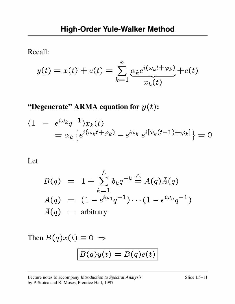
High-Order Yule-Walker Method
Recall:
y(t) = x(t) + e(t) =nX
k=1
�kei(!kt+'k)| {z }xk(t)
+e(t)
“Degenerate” ARMA equation for y(t):
(1 � ei!kq�1)xk(t)
= �knei(!kt+'k) � ei!k ei[!k(t�1)+'k]
o= 0
Let
B(q) = 1+LX
k=1
bkq�k 4= A(q) �A(q)
A(q) = (1� ei!1q�1) � � � (1� ei!nq�1)
�A(q) = arbitrary
Then B(q)x(t) � 0 )
B(q)y(t) = B(q)e(t)
Lecture notes to accompany Introduction to Spectral Analysis Slide L5–11by P. Stoica and R. Moses, Prentice Hall, 1997
High-Order Yule-Walker Method, con't
Estimation Procedure:
� Estimate fbigLi=1 using an ARMA MYW technique
� Roots of B(q) give f!kgnk=1, along with L� n
“spurious” roots.
Lecture notes to accompany Introduction to Spectral Analysis Slide L5–12by P. Stoica and R. Moses, Prentice Hall, 1997

High-Order and Overdetermined YW Equations
ARMA covariance:
r(k) +LXi=1
bir(k � i) = 0; k > L
In matrix form for k = L+1; : : : ; L+M
26664
r(L) : : : r(1)r(L+1) : : : r(2)
... ...r(L+M � 1) : : : r(M)
37775
| {z }4=
b = �
26664r(L+1)r(L+2)
...r(L+M)
37775
| {z }4=�
This is a high-order (if L > n) and overdetermined
(if M > L) system of YW equations.
Lecture notes to accompany Introduction to Spectral Analysis Slide L5–13by P. Stoica and R. Moses, Prentice Hall, 1997
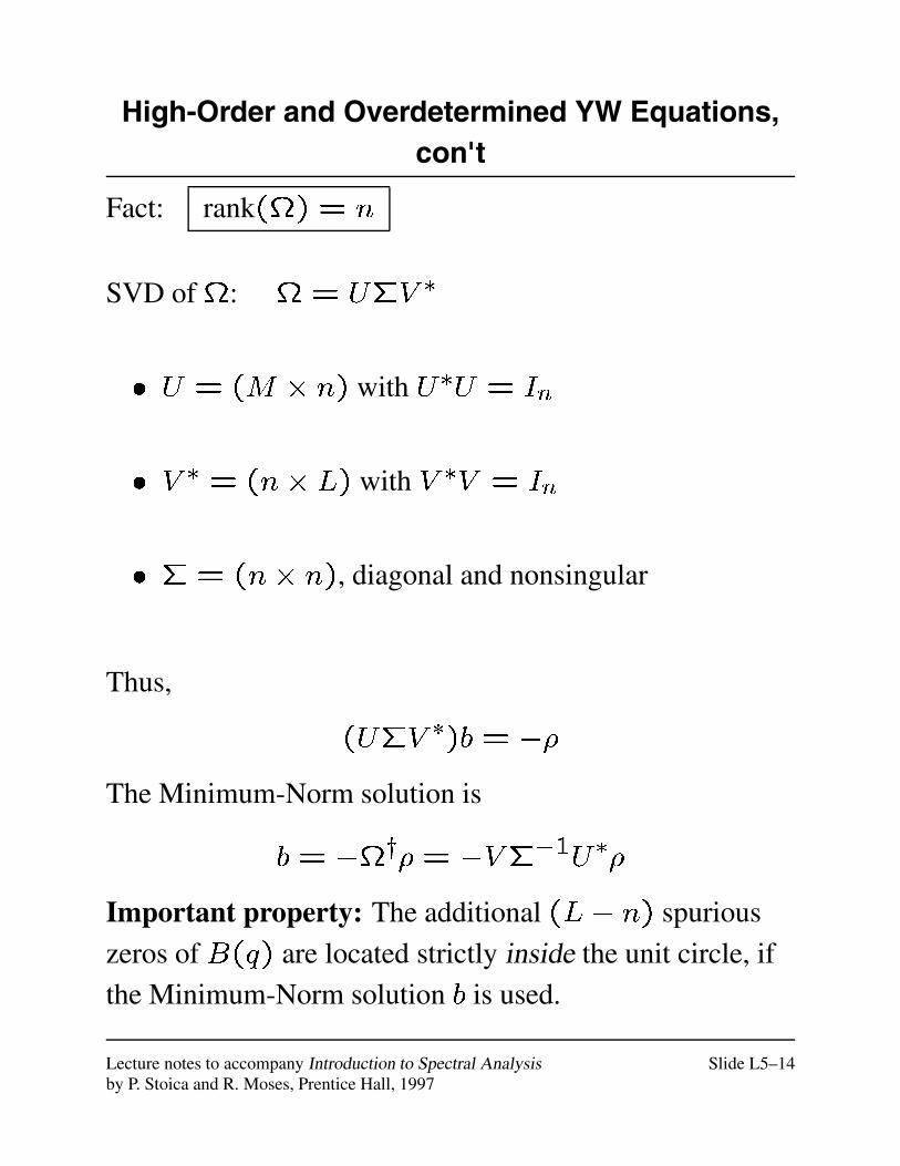
High-Order and Overdetermined YW Equations,con't
Fact: rank() = n
SVD of : = U�V �
� U = (M � n) with U�U = In
� V � = (n� L) with V �V = In
� � = (n� n), diagonal and nonsingular
Thus,
(U�V �)b = ��
The Minimum-Norm solution is
b = �y�= �V��1U��
Important property: The additional (L� n) spurious
zeros of B(q) are located strictly inside the unit circle, if
the Minimum-Norm solution b is used.
Lecture notes to accompany Introduction to Spectral Analysis Slide L5–14by P. Stoica and R. Moses, Prentice Hall, 1997
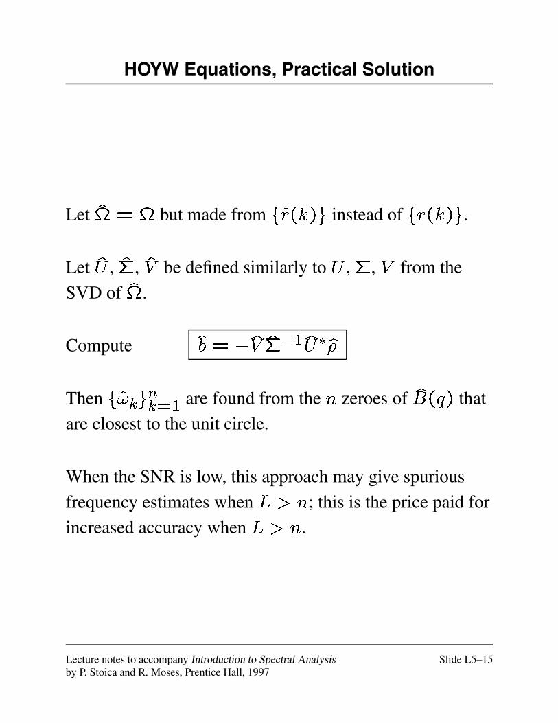
HOYW Equations, Practical Solution
Let = but made from fr(k)g instead of fr(k)g.
Let U , �, V be defined similarly to U , �, V from the
SVD of .
Compute b = �V ��1U��
Then f!kgnk=1 are found from the n zeroes of B(q) that
are closest to the unit circle.
When the SNR is low, this approach may give spurious
frequency estimates when L > n; this is the price paid for
increased accuracy when L > n.
Lecture notes to accompany Introduction to Spectral Analysis Slide L5–15by P. Stoica and R. Moses, Prentice Hall, 1997
Parametric Methods
for
Line Spectra — Part 2
Lecture 6
Lecture notes to accompany Introduction to Spectral Analysis Slide L6–1by P. Stoica and R. Moses, Prentice Hall, 1997
The Covariance Matrix Equation
Let:
a(!) = [1 e�i! : : : e�i(m�1)!]T
A = [a(!1) : : : a(!n)] (m� n)
Note: rank(A) = n (for m � n )
Define
~y(t)4=
26664
y(t)y(t� 1)
...y(t�m+1)
37775 = A~x(t) + ~e(t)
where
~x(t) = [x1(t) : : : xn(t)]T
~e(t) = [e(t) : : : e(t�m+1)]T
Then
R4= E f~y(t)~y�(t)g = APA�+ �2I
with
P = E f~x(t)~x�(t)g =
264 �
21 0
. . .0 �2n
375
Lecture notes to accompany Introduction to Spectral Analysis Slide L6–2by P. Stoica and R. Moses, Prentice Hall, 1997
Eigendecomposition of R and Its Properties
R = APA�+ �2I (m > n)
Let:
�1 � �2 � : : : � �m: eigenvalues of R
fs1; : : : sng: orthonormal eigenvectors associated
with f�1; : : : ; �ng
fg1; : : : ; gm�ng: orthonormal eigenvectors associated
with f�n+1; : : : ; �mg
S = [s1 : : : sn] (m� n)
G = [g1 : : : gm�n] (m� (m� n))
Thus,
R = [S G]
264 �1 . . .
�m
375"S�
G�
#
Lecture notes to accompany Introduction to Spectral Analysis Slide L6–3by P. Stoica and R. Moses, Prentice Hall, 1997
Eigendecomposition of R and Its Properties,con't
As rank(APA�) = n:
�k > �2 k = 1; : : : ; n
�k = �2 k = n+1; : : : ;m
��=
264 �1 � �
2 0. . .
0 �n � �2
375 = nonsingular
Note:
RS = APA�S+ �2S = S
264 �1 0
. . .0 �n
375
S = A(PA�S�� �1)
4= AC
with jCj 6= 0 (since rank(S) = rank(A) = n).
Therefore, since S�G= 0,
A�G = 0
Lecture notes to accompany Introduction to Spectral Analysis Slide L6–4by P. Stoica and R. Moses, Prentice Hall, 1997
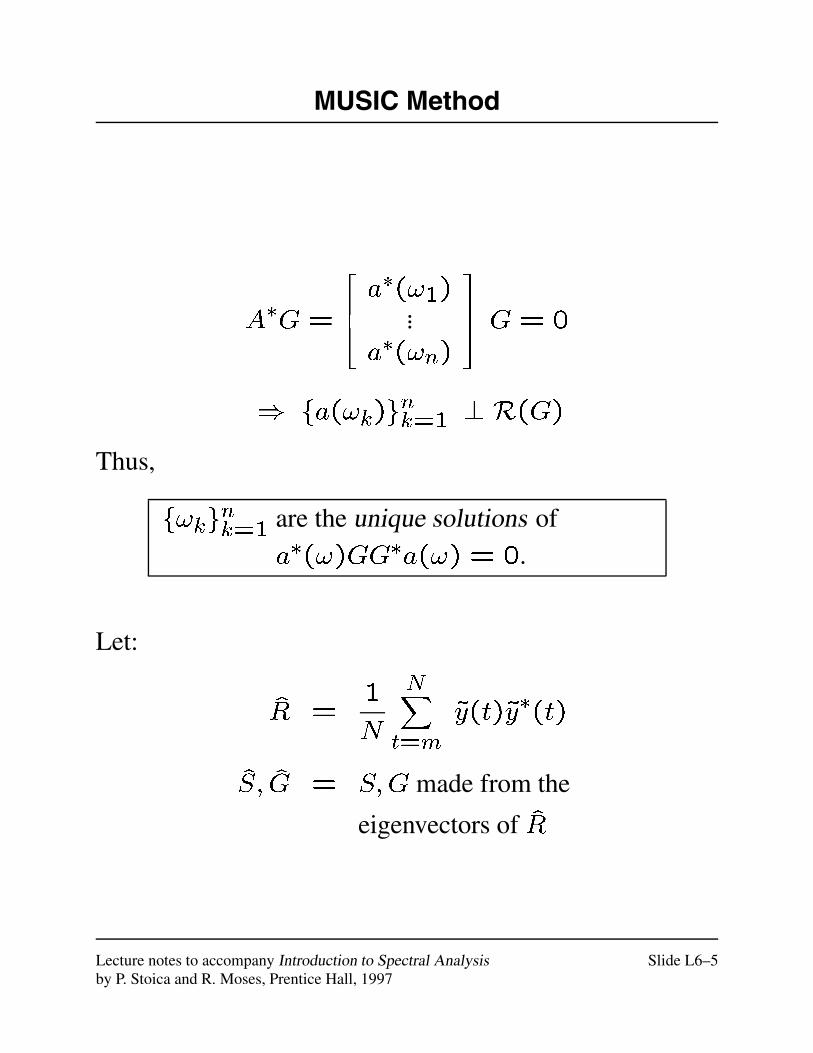
MUSIC Method
A�G=
264 a
�(!1)...
a�(!n)
375 G = 0
) fa(!k)gnk=1 ? R(G)
Thus,
f!kgnk=1 are the unique solutions of
a�(!)GG�a(!) = 0.
Let:
R =1
N
NXt=m
~y(t)~y�(t)
S; G = S;G made from the
eigenvectors of R
Lecture notes to accompany Introduction to Spectral Analysis Slide L6–5by P. Stoica and R. Moses, Prentice Hall, 1997
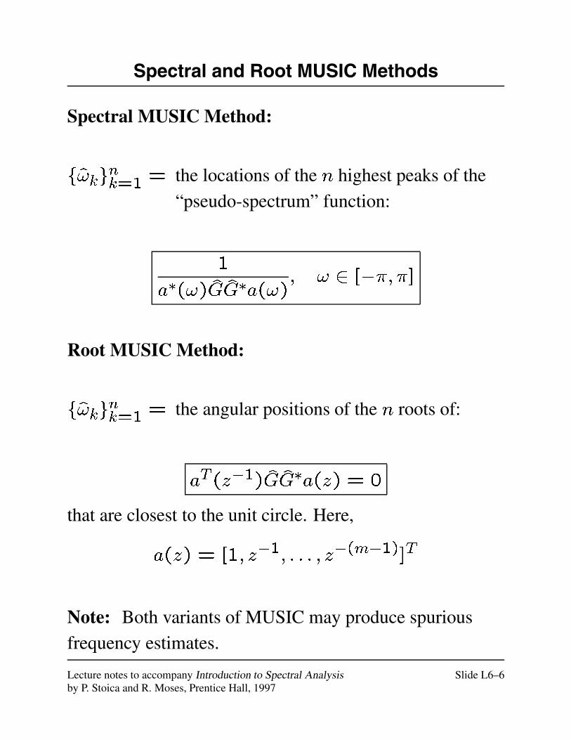
Spectral and Root MUSIC Methods
Spectral MUSIC Method:
f!kgnk=1 = the locations of the n highest peaks of the
“pseudo-spectrum” function:
1
a�(!)GG�a(!); ! 2 [��; �]
Root MUSIC Method:
f!kgnk=1 = the angular positions of the n roots of:
aT (z�1)GG�a(z) = 0
that are closest to the unit circle. Here,
a(z) = [1; z�1; : : : ; z�(m�1)]T
Note: Both variants of MUSIC may produce spuriousfrequency estimates.
Lecture notes to accompany Introduction to Spectral Analysis Slide L6–6by P. Stoica and R. Moses, Prentice Hall, 1997
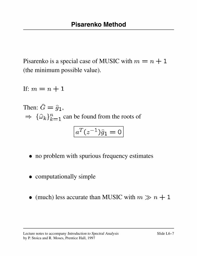
Pisarenko Method
Pisarenko is a special case of MUSIC with m = n+1
(the minimum possible value).
If: m = n+1
Then: G = g1,
) f!kgnk=1 can be found from the roots of
aT (z�1)g1 = 0
� no problem with spurious frequency estimates
� computationally simple
� (much) less accurate than MUSIC with m� n+1
Lecture notes to accompany Introduction to Spectral Analysis Slide L6–7by P. Stoica and R. Moses, Prentice Hall, 1997
Min-Norm Method
Goals: Reduce computational burden, and reduce risk of
false frequency estimates.
Uses m� n (as in MUSIC), but only one vector in
R(G) (as in Pisarenko).
Let "1g
#= the vector in R(G), with first element equal
to one, that has minimum Euclidean norm.
Lecture notes to accompany Introduction to Spectral Analysis Slide L6–8by P. Stoica and R. Moses, Prentice Hall, 1997
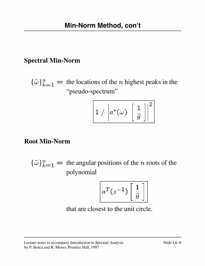
Min-Norm Method, con't
Spectral Min-Norm
f!gnk=1 = the locations of the n highest peaks in the
“pseudo-spectrum”
1 =
�����a�(!)"1g
#�����2
Root Min-Norm
f!gnk=1 = the angular positions of the n roots of the
polynomial
aT (z�1)
"1g
#
that are closest to the unit circle.
Lecture notes to accompany Introduction to Spectral Analysis Slide L6–9by P. Stoica and R. Moses, Prentice Hall, 1997
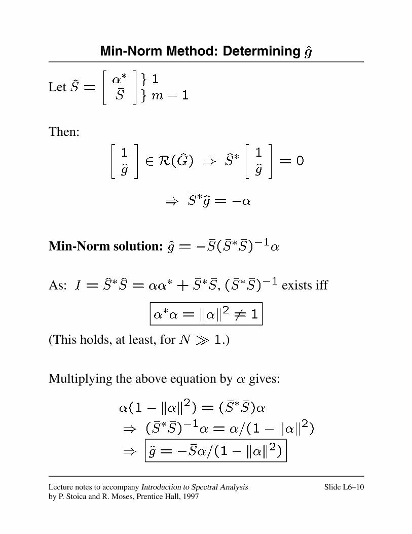
Min-Norm Method: Determining g
Let S =
"��
�S
#g 1g m� 1
Then: "1g
#2 R(G) ) S�
"1g
#= 0
) �S�g = ��
Min-Norm solution: g = ��S(�S��S)�1�
As: I = S�S = ���+ �S��S, (�S��S)�1 exists iff
��� = k�k2 6= 1
(This holds, at least, for N � 1.)
Multiplying the above equation by � gives:
�(1� k�k2) = (�S��S)�
) (�S��S)�1� = �=(1� k�k2)
) g = ��S�=(1� k�k2)
Lecture notes to accompany Introduction to Spectral Analysis Slide L6–10by P. Stoica and R. Moses, Prentice Hall, 1997
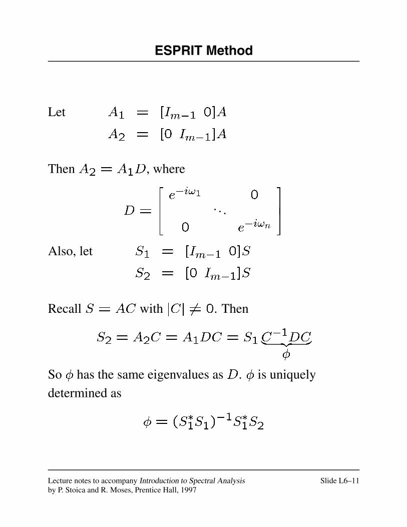
ESPRIT Method
Let A1 = [Im�1 0]A
A2 = [0 Im�1]A
Then A2 = A1D, where
D =
264 e
�i!1 0. . .
0 e�i!n
375
Also, let S1 = [Im�1 0]S
S2 = [0 Im�1]S
Recall S = AC with jCj 6= 0. Then
S2 = A2C = A1DC = S1C�1DC| {z }�
So � has the same eigenvalues as D. � is uniquely
determined as
� = (S�1S1)�1S�1S2
Lecture notes to accompany Introduction to Spectral Analysis Slide L6–11by P. Stoica and R. Moses, Prentice Hall, 1997
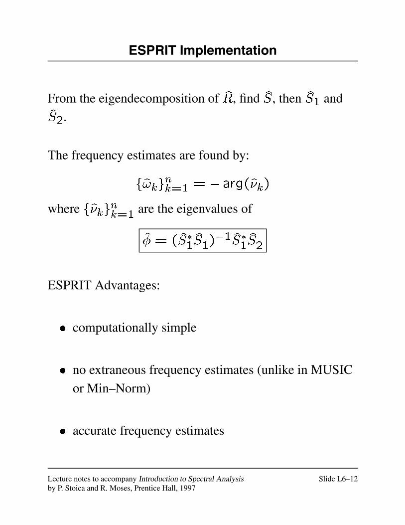
ESPRIT Implementation
From the eigendecomposition of R, find S, then S1 and
S2.
The frequency estimates are found by:
f!kgnk=1 = �arg(�k)
where f�kgnk=1 are the eigenvalues of
� = (S�1S1)�1S�1S2
ESPRIT Advantages:
� computationally simple
� no extraneous frequency estimates (unlike in MUSIC
or Min–Norm)
� accurate frequency estimates
Lecture notes to accompany Introduction to Spectral Analysis Slide L6–12by P. Stoica and R. Moses, Prentice Hall, 1997
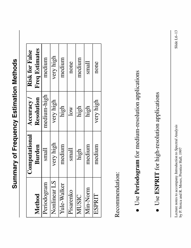
Su
mm
ary
of
Fre
qu
ency
Est
imat
ion
Met
ho
ds
Com
puta
tion
alA
ccur
acy
/R
isk
for
Fal
seM
etho
dB
urde
nR
esol
utio
nF
req
Est
imat
esPe
riod
ogra
msm
all
med
ium
-hig
hm
ediu
mN
onlin
ear
LS
very
high
very
high
very
high
Yul
e-W
alke
rm
ediu
mhi
ghm
ediu
mPi
sare
nko
smal
llo
wno
neM
USI
Chi
ghhi
ghm
ediu
mM
in-N
orm
med
ium
high
smal
lE
SPR
ITm
ediu
mve
ryhi
ghno
ne
Rec
omm
enda
tion:
�
Use
Per
iodo
gram
for
med
ium
-res
olut
ion
appl
icat
ions
�
Use
ESP
RIT
for
high
-res
olut
ion
appl
icat
ions
Lec
ture
note
sto
acco
mpa
nyIn
trod
uctio
nto
Spec
tral
Ana
lysi
sSl
ide
L6–
13by
P.St
oica
and
R.M
oses
,Pre
ntic
eH
all,
1997
Filter Bank Methods
Lecture 7
Lecture notes to accompany Introduction to Spectral Analysis Slide L7–1by P. Stoica and R. Moses, Prentice Hall, 1997
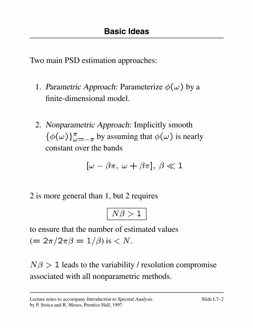
Basic Ideas
Two main PSD estimation approaches:
1. Parametric Approach: Parameterize �(!) by a
finite-dimensional model.
2. Nonparametric Approach: Implicitly smooth
f�(!)g�!=�� by assuming that �(!) is nearly
constant over the bands
[! � ��; !+ ��]; � � 1
2 is more general than 1, but 2 requires
N� > 1
to ensure that the number of estimated values
(= 2�=2�� = 1=�) is < N .
N� > 1 leads to the variability / resolution compromise
associated with all nonparametric methods.
Lecture notes to accompany Introduction to Spectral Analysis Slide L7–2by P. Stoica and R. Moses, Prentice Hall, 1997
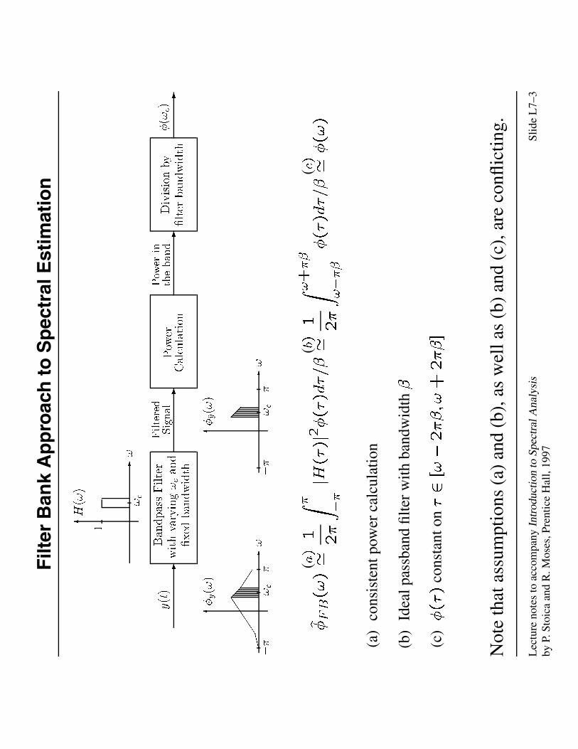
Filt
erB
ank
Ap
pro
ach
toS
pec
tral
Est
imat
ion
-
-
-
-
Divisionby
�lterbandwidth
Power
Calculation
BandpassFilter
withvarying!c
and
�xedbandwidth
^ �(!c)
Powerin
theband
Filtered
Signal
y(t)
-
6
�
�
!c
�
!
�y(!)
��
����
-
6
�
�
!c
�
!
�~y(!)
@ @
-
61
!c
!
H(!)
^ �FB(!)
(a)'
1 2�
Z � ��
jH(�)j2�(�)d�=�
(b)'
1 2�
Z !+��
!���
�(�)d�=�
(c)'�(!)
(a)
cons
iste
ntpo
wer
calc
ulat
ion
(b)
Idea
lpas
sban
dfil
ter
with
band
wid
th�
(c)
�(�)
cons
tant
on
�2[!�2��;!+2��]
Not
eth
atas
sum
ptio
ns(a
)an
d(b
),as
wel
las
(b)
and
(c),
are
confl
ictin
g.
Lec
ture
note
sto
acco
mpa
nyIn
trod
uctio
nto
Spec
tral
Ana
lysi
sSl
ide
L7–
3by
P.St
oica
and
R.M
oses
,Pre
ntic
eH
all,
1997
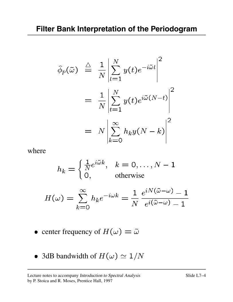
Filter Bank Interpretation of the Periodogram
�p(~!)4=
1
N
������NXt=1
y(t)e�i~!t
������2
=1
N
������NXt=1
y(t)ei~!(N�t)
������2
= N
������1Xk=0
hky(N � k)
������2
where
hk =
(1N e
i~!k; k = 0; : : : ; N � 1
0; otherwise
H(!) =1Xk=0
hke�i!k =
1
N
eiN(~!�!) � 1
ei(~!�!) � 1
� center frequency of H(!) = ~!
� 3dB bandwidth of H(!) ' 1=N
Lecture notes to accompany Introduction to Spectral Analysis Slide L7–4by P. Stoica and R. Moses, Prentice Hall, 1997
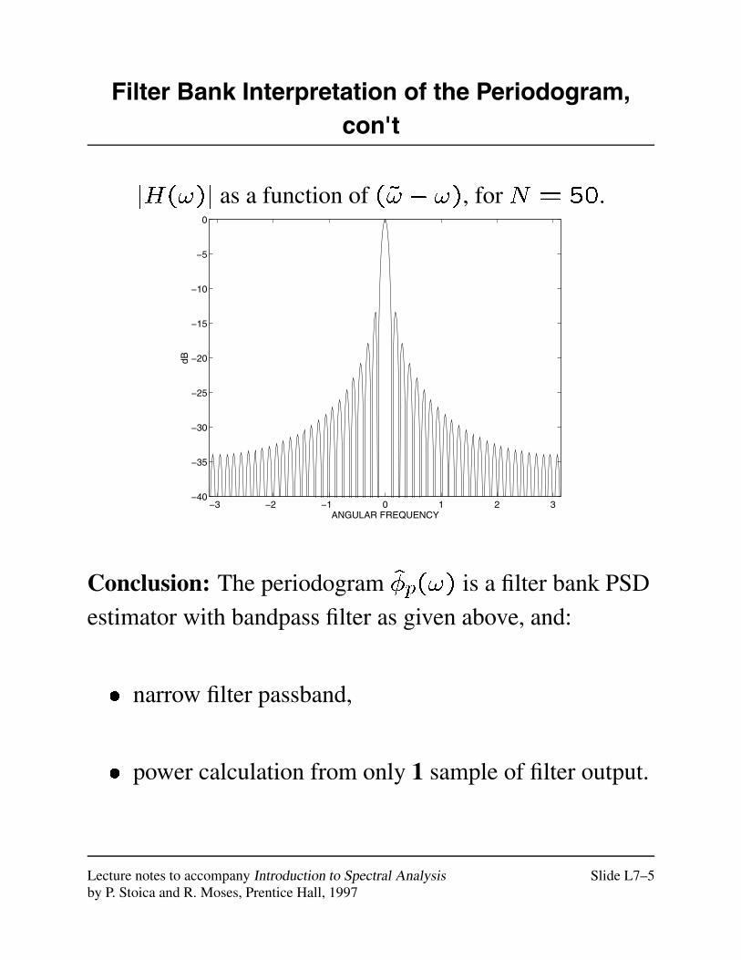
Filter Bank Interpretation of the Periodogram,con't
jH(!)j as a function of (~! � !), for N = 50.
−3 −2 −1 0 1 2 3−40
−35
−30
−25
−20
−15
−10
−5
0
dB
ANGULAR FREQUENCY
Conclusion: The periodogram �p(!) is a filter bank PSD
estimator with bandpass filter as given above, and:
� narrow filter passband,
� power calculation from only 1 sample of filter output.
Lecture notes to accompany Introduction to Spectral Analysis Slide L7–5by P. Stoica and R. Moses, Prentice Hall, 1997

Possible Improvements to the Filter BankApproach
1. Split the available sample, and bandpass filter each
subsample.
� more data points for the power calculation stage.
This approach leads to Bartlett and Welch methods.
2. Use several bandpass filters on the whole sample.
Each filter covers a small band centered on ~!.
� provides several samples for power calculation.
This “multiwindow approach” is similar to the
Daniell method.
Both approaches compromise bias for variance, and in fact
are quite related to each other: splitting the data sample
can be interpreted as a special form of windowing or
filtering.
Lecture notes to accompany Introduction to Spectral Analysis Slide L7–6by P. Stoica and R. Moses, Prentice Hall, 1997
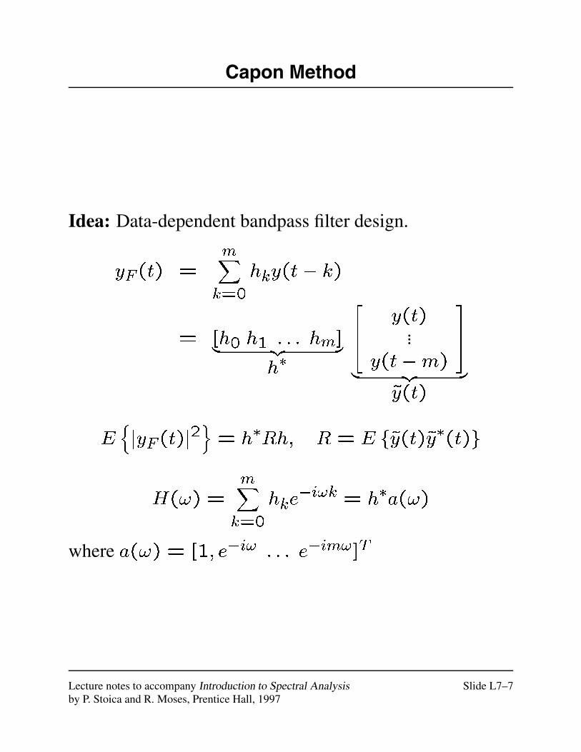
Capon Method
Idea: Data-dependent bandpass filter design.
yF(t) =mXk=0
hky(t� k)
= [h0 h1 : : : hm]| {z }h�
264 y(t)
...y(t�m)
375
| {z }~y(t)
EnjyF(t)j
2o= h�Rh; R = E f~y(t)~y�(t)g
H(!) =mXk=0
hke�i!k = h�a(!)
where a(!) = [1; e�i! : : : e�im!]T
Lecture notes to accompany Introduction to Spectral Analysis Slide L7–7by P. Stoica and R. Moses, Prentice Hall, 1997
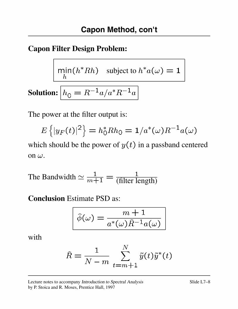
Capon Method, con't
Capon Filter Design Problem:
minh(h�Rh) subject to h�a(!) = 1
Solution: h0 = R�1a=a�R�1a
The power at the filter output is:
EnjyF(t)j
2o= h�0Rh0 = 1=a�(!)R�1a(!)
which should be the power of y(t) in a passband centeredon !.
The Bandwidth' 1m+1 =
1(filter length)
Conclusion Estimate PSD as:
�(!) =m+1
a�(!)R�1a(!)
with
R =1
N �m
NXt=m+1
~y(t)~y�(t)
Lecture notes to accompany Introduction to Spectral Analysis Slide L7–8by P. Stoica and R. Moses, Prentice Hall, 1997
Capon Properties
� m is the user parameter that controls the compromise
between bias and variance:
– as m increases, bias decreases and variance
increases.
� Capon uses one bandpass filter only, but it splits the
N -data point sample into (N �m) subsequences of
length m with maximum overlap.
Lecture notes to accompany Introduction to Spectral Analysis Slide L7–9by P. Stoica and R. Moses, Prentice Hall, 1997
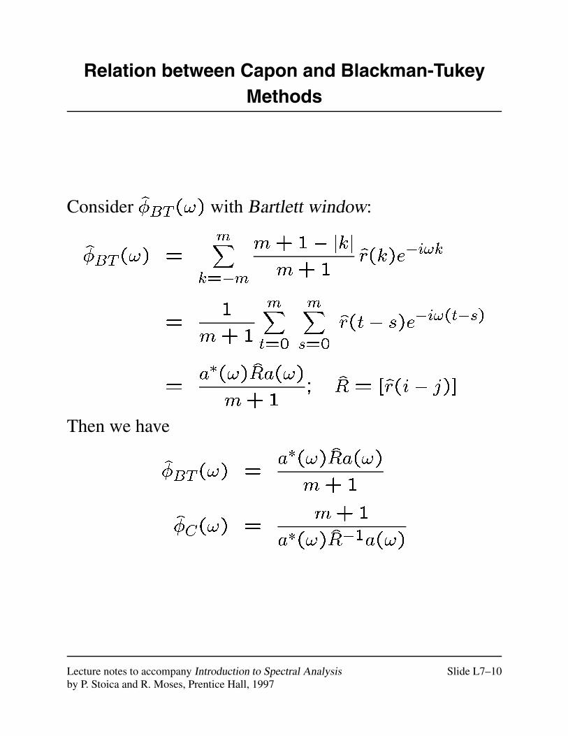
Relation between Capon and Blackman-TukeyMethods
Consider �BT (!) with Bartlett window:
�BT (!) =mX
k=�m
m+1� jkj
m+1r(k)e�i!k
=1
m+1
mXt=0
mXs=0
r(t� s)e�i!(t�s)
=a�(!)Ra(!)
m+1; R = [r(i� j)]
Then we have
�BT (!) =a�(!)Ra(!)
m+1
�C(!) =m+1
a�(!)R�1a(!)
Lecture notes to accompany Introduction to Spectral Analysis Slide L7–10by P. Stoica and R. Moses, Prentice Hall, 1997
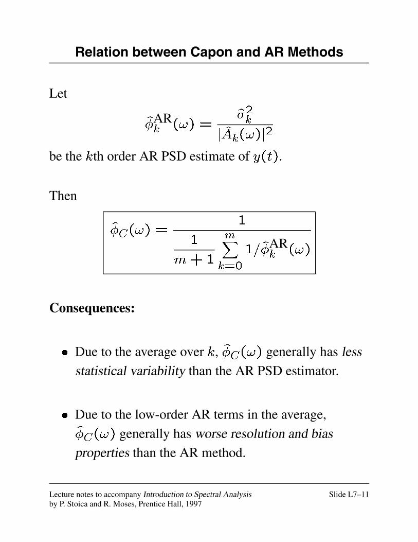
Relation between Capon and AR Methods
Let
�ARk (!) =
�2kjAk(!)j
2
be the kth order AR PSD estimate of y(t).
Then
�C(!) =1
1
m+1
mXk=0
1=�ARk (!)
Consequences:
� Due to the average over k, �C(!) generally has lessstatistical variability than the AR PSD estimator.
� Due to the low-order AR terms in the average,
�C(!) generally has worse resolution and biasproperties than the AR method.
Lecture notes to accompany Introduction to Spectral Analysis Slide L7–11by P. Stoica and R. Moses, Prentice Hall, 1997
Spatial Methods — Part 1
Lecture 8
Lecture notes to accompany Introduction to Spectral Analysis Slide L8–1by P. Stoica and R. Moses, Prentice Hall, 1997
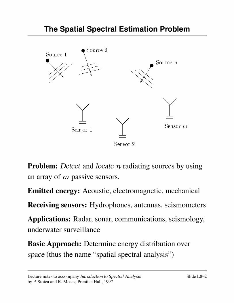
The Spatial Spectral Estimation Problem
Source n
Source 2Source 1
�
BBBBBN
@@@@R
v
v
v
Sensor 1
@@ ��
@@ ��
@@ ��
Sensor 2
Sensor m
ccccc
cccc
ccc
������������,
,,
,,
,,,
,,
,,
Problem: Detect and locate n radiating sources by using
an array of m passive sensors.
Emitted energy: Acoustic, electromagnetic, mechanical
Receiving sensors: Hydrophones, antennas, seismometers
Applications: Radar, sonar, communications, seismology,
underwater surveillance
Basic Approach: Determine energy distribution over
space (thus the name “spatial spectral analysis”)
Lecture notes to accompany Introduction to Spectral Analysis Slide L8–2by P. Stoica and R. Moses, Prentice Hall, 1997
Simplifying Assumptions
� Far-field sources in the same plane as the array of
sensors
� Non-dispersive wave propagation
Hence: The waves are planar and the only location
parameter is direction of arrival (DOA)(or angle of arrival, AOA).
� The number of sources n is known. (We do not treat
the detection problem)
� The sensors are linear dynamic elements with knowntransfer characteristics and known locations
(That is, the array is calibrated.)
Lecture notes to accompany Introduction to Spectral Analysis Slide L8–3by P. Stoica and R. Moses, Prentice Hall, 1997

Array Model — Single Emitter Case
x(t) = the signal waveform as measured at a referencepoint (e.g., at the “first” sensor)
�k = the delay between the reference point and thekth sensor
hk(t) = the impulse response (weighting function) ofsensor k
�ek(t) = “noise” at the kth sensor (e.g., thermal noise insensor electronics; background noise, etc.)
Note: t 2 R (continuous-time signals).
Then the output of sensor k is
�yk(t) = hk(t) � x(t� �k) + �ek(t)
(� = convolution operator).
Basic Problem: Estimate the time delays f�kg with hk(t)known but x(t) unknown.
This is a time-delay estimation problem in the unknowninput case.
Lecture notes to accompany Introduction to Spectral Analysis Slide L8–4by P. Stoica and R. Moses, Prentice Hall, 1997
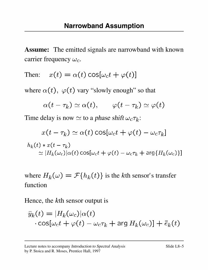
Narrowband Assumption
Assume: The emitted signals are narrowband with known
carrier frequency !c.
Then: x(t) = �(t) cos[!ct+ '(t)]
where �(t); '(t) vary “slowly enough” so that
�(t� �k) ' �(t); '(t� �k) ' '(t)
Time delay is now' to a phase shift !c�k:
x(t� �k) ' �(t) cos[!ct+ '(t)� !c�k]
hk(t) � x(t� �k)
' jHk(!c)j�(t) cos[!ct+ '(t)� !c�k +argfHk(!c)g]
where Hk(!) = Ffhk(t)g is the kth sensor's transfer
function
Hence, the kth sensor output is
�yk(t) = jHk(!c)j�(t)
� cos[!ct+ '(t)� !c�k+ argHk(!c)] + �ek(t)
Lecture notes to accompany Introduction to Spectral Analysis Slide L8–5by P. Stoica and R. Moses, Prentice Hall, 1997
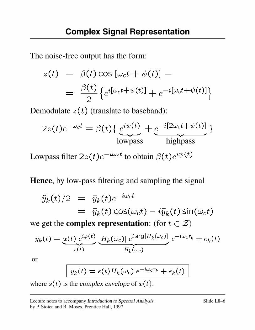
Complex Signal Representation
The noise-free output has the form:
z(t) = �(t) cos [!ct+ (t)] =
=�(t)
2
nei[!ct+ (t)]+ e�i[!ct+ (t)]
oDemodulate z(t) (translate to baseband):
2z(t)e�!ct = �(t)f ei (t)| {z }lowpass
+ e�i[2!ct+ (t)]| {z }highpass
g
Lowpass filter 2z(t)e�i!ct to obtain �(t)ei (t)
Hence, by low-pass filtering and sampling the signal
~yk(t)=2 = �yk(t)e�i!ct
= �yk(t) cos(!ct)� i�yk(t) sin(!ct)
we get the complex representation: (for t 2 Z)
yk(t) = �(t) ei'(t)| {z }s(t)
jHk(!c)j eiarg[Hk(!c)]| {z }
Hk(!c)
e�i!c�k + ek(t)
or
yk(t) = s(t)Hk(!c) e�i!c�k + ek(t)
where s(t) is the complex envelope of x(t).
Lecture notes to accompany Introduction to Spectral Analysis Slide L8–6by P. Stoica and R. Moses, Prentice Hall, 1997
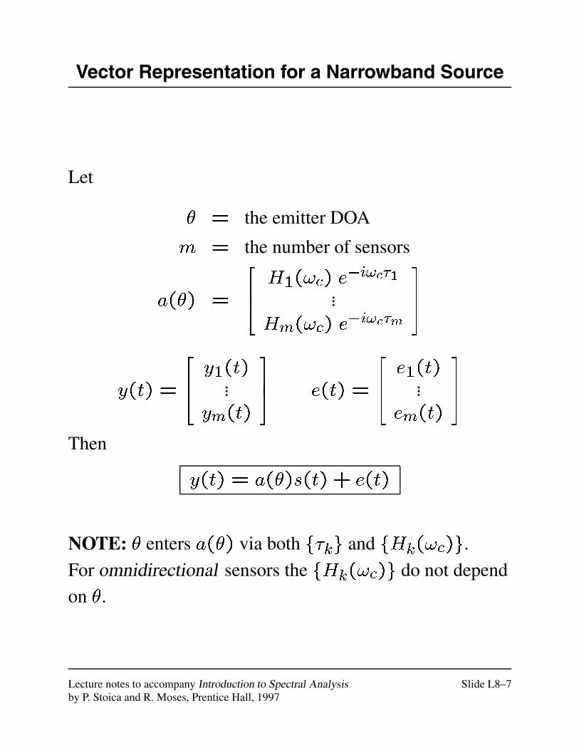
Vector Representation for a Narrowband Source
Let
� = the emitter DOA
m = the number of sensors
a(�) =
264 H1(!c) e
�i!c�1...
Hm(!c) e�i!c�m
375
y(t) =
264 y1(t)
...ym(t)
375 e(t) =
264 e1(t)
...em(t)
375
Then
y(t) = a(�)s(t) + e(t)
NOTE: � enters a(�) via both f�kg and fHk(!c)g.
For omnidirectional sensors the fHk(!c)g do not depend
on �.
Lecture notes to accompany Introduction to Spectral Analysis Slide L8–7by P. Stoica and R. Moses, Prentice Hall, 1997
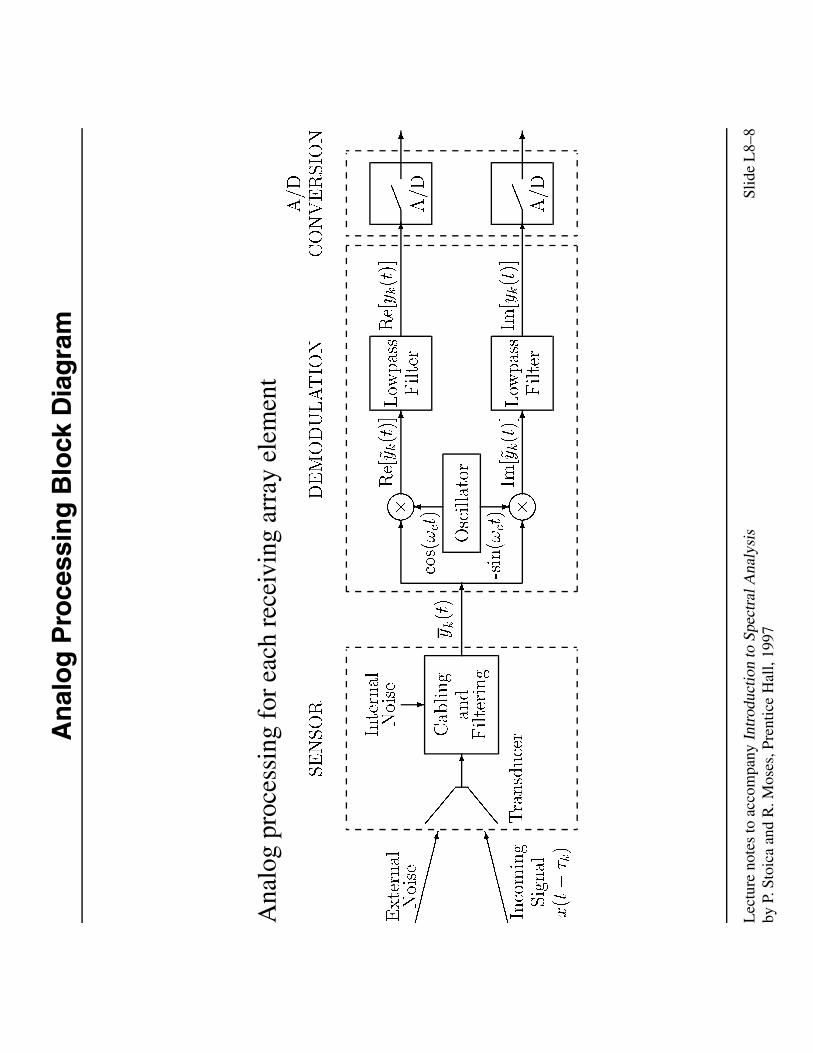
An
alo
gP
roce
ssin
gB
lock
Dia
gra
m
Ana
log
proc
essi
ngfo
rea
chre
ceiv
ing
arra
yel
emen
t
XXXXXXXz
�������:
External
Noise
Incoming
Signal
x(t�
�k)
SENSOR
,,,
lll
-
Cabling
and
Filtering
?
Internal
Noise
Transducer
-
yk(t)
DEMODULATION
��
��
��
����
Oscillator
Lowpass
Filter
Lowpass
Filter
- -
6 ?
-sin(!ct)
cos(!ct)
- -
Im[yk(t)]
Re[yk(t)]
- -
Im[~yk(t)]
Re[~y k(t)]
A/D
CONVERSION
!!
!!
- -
A/D
A/D
Lec
ture
note
sto
acco
mpa
nyIn
trod
uctio
nto
Spec
tral
Ana
lysi
sSl
ide
L8–
8by
P.St
oica
and
R.M
oses
,Pre
ntic
eH
all,
1997
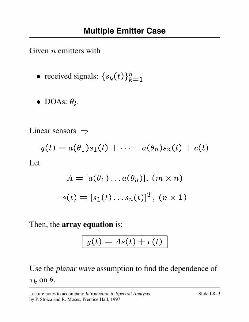
Multiple Emitter Case
Given n emitters with
� received signals: fsk(t)gnk=1
� DOAs: �k
Linear sensors )
y(t) = a(�1)s1(t) + � � �+ a(�n)sn(t) + e(t)
Let
A = [a(�1) : : : a(�n)]; (m� n)
s(t) = [s1(t) : : : sn(t)]T ; (n� 1)
Then, the array equation is:
y(t) = As(t) + e(t)
Use the planar wave assumption to find the dependence of�k on �.
Lecture notes to accompany Introduction to Spectral Analysis Slide L8–9by P. Stoica and R. Moses, Prentice Hall, 1997
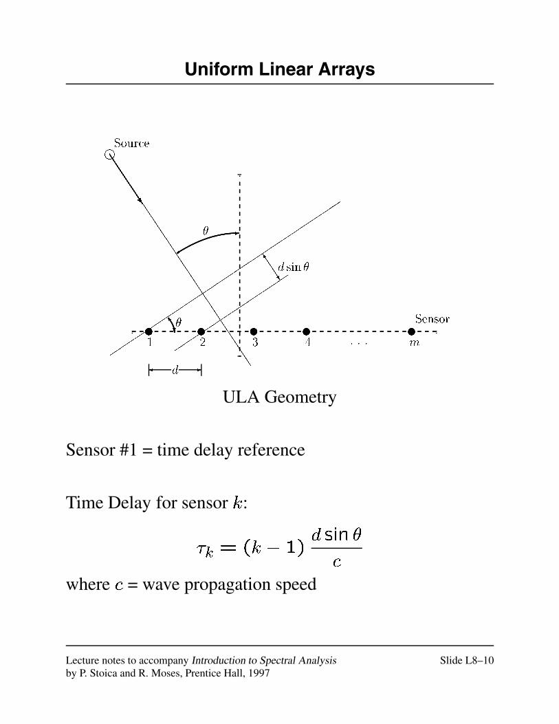
Uniform Linear Arrays
�����������������������
Source
-
+
�
?]�
p p p
Sensor
m4321
d sin �JJJJ]
d -�
�����������
JJJJJJJJJJJJJJJJJJJJJ
JJJJJ
h
v v v v v
ULA Geometry
Sensor #1 = time delay reference
Time Delay for sensor k:
�k = (k � 1)d sin �
c
where c = wave propagation speed
Lecture notes to accompany Introduction to Spectral Analysis Slide L8–10by P. Stoica and R. Moses, Prentice Hall, 1997
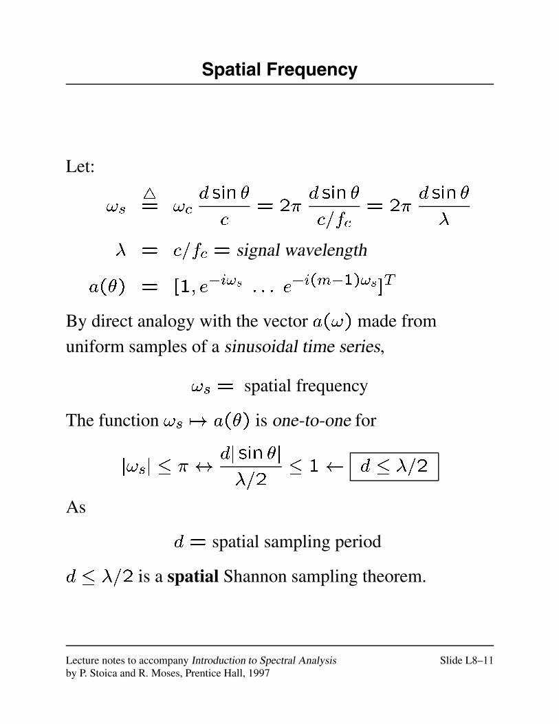
Spatial Frequency
Let:
!s4= !c
d sin �
c= 2�
d sin �
c=fc= 2�
d sin �
�
� = c=fc = signal wavelength
a(�) = [1; e�i!s : : : e�i(m�1)!s]T
By direct analogy with the vector a(!) made from
uniform samples of a sinusoidal time series,
!s = spatial frequency
The function !s 7! a(�) is one-to-one for
j!sj � � $dj sin �j
�=2� 1 d � �=2
As
d = spatial sampling period
d � �=2 is a spatial Shannon sampling theorem.
Lecture notes to accompany Introduction to Spectral Analysis Slide L8–11by P. Stoica and R. Moses, Prentice Hall, 1997
Spatial Methods — Part 2
Lecture 9
Lecture notes to accompany Introduction to Spectral Analysis Slide L9–1by P. Stoica and R. Moses, Prentice Hall, 1997
Spatial Filtering
Spatial filtering useful for
� DOA discrimination (similar to frequency
discrimination of time-series filtering)
� Nonparametric DOA estimation
There is a strong analogy between temporal filtering and
spatial filtering.
Lecture notes to accompany Introduction to Spectral Analysis Slide L9–2by P. Stoica and R. Moses, Prentice Hall, 1997
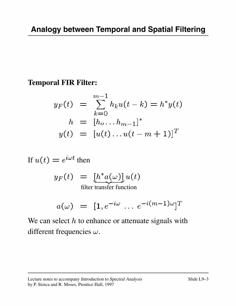
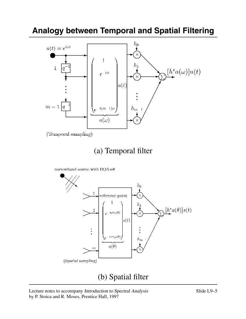
Analogy between Temporal and Spatial Filtering
Temporal FIR Filter:
yF(t) =m�1Xk=0
hku(t� k) = h�y(t)
h = [ho : : : hm�1]�
y(t) = [u(t) : : : u(t�m+1)]T
If u(t) = ei!t then
yF(t) = [h�a(!)]| {z }filter transfer function
u(t)
a(!) = [1; e�i! : : : e�i(m�1)!]T
We can select h to enhance or attenuate signals with
different frequencies !.
Lecture notes to accompany Introduction to Spectral Analysis Slide L9–3by P. Stoica and R. Moses, Prentice Hall, 1997
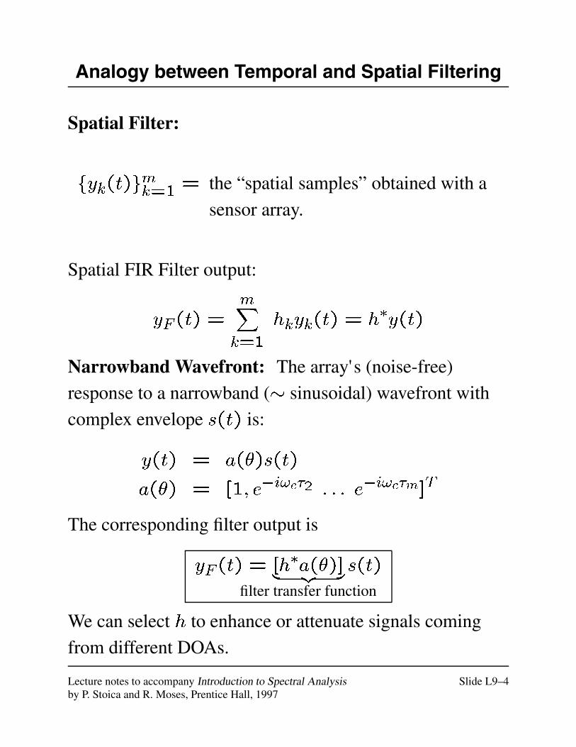
Analogy between Temporal and Spatial Filtering
Spatial Filter:
fyk(t)gmk=1 = the “spatial samples” obtained with a
sensor array.
Spatial FIR Filter output:
yF(t) =mXk=1
hkyk(t) = h�y(t)
Narrowband Wavefront: The array's (noise-free)
response to a narrowband (� sinusoidal) wavefront with
complex envelope s(t) is:
y(t) = a(�)s(t)
a(�) = [1; e�i!c�2 : : : e�i!c�m]T
The corresponding filter output is
yF(t) = [h�a(�)]| {z }filter transfer function
s(t)
We can select h to enhance or attenuate signals coming
from different DOAs.
Lecture notes to accompany Introduction to Spectral Analysis Slide L9–4by P. Stoica and R. Moses, Prentice Hall, 1997
Analogy between Temporal and Spatial Filtering
(Temporal sampling)
z
-
qqq
?
?
?
����������
-
-
-
-
� ��
� ��
� ��
� ��
@@@@@R
-
?
?
qqq
-s
-
?
s
�
�
�
P
u(t) = ei!t
q�1
q�1
1
m� 1
0BBBBBBBBBBBBBB@
1
e�i!
...
e�i(m�1)!
1CCCCCCCCCCCCCCA
| {z }a(!)
u(t)
h0
h1
hm�1
[h�a(!)]u(t)
(a) Temporal filter
ZZZZZ~
��
��
�����
���
narrowband source with DOA=�
(Spatial sampling)
�
�
�
P
z
-
qqq
?
?
?
����������
@@@@@R-
-
-
-
� ��
� ��
� ��
� ��
-!!aa
-!!aa
-!!aa
qqq
reference point1
2
m
0BBBBBBBBBBB@
1
e�i!�2(�)
...
e�i!�m(�)
1CCCCCCCCCCCA
| {z }a(�)
s(t)
h0
h1
hm�1
[h�a(�)]s(t)
(b) Spatial filter
Lecture notes to accompany Introduction to Spectral Analysis Slide L9–5by P. Stoica and R. Moses, Prentice Hall, 1997
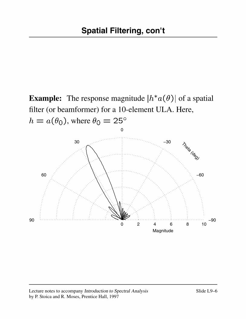
Spatial Filtering, con't
Example: The response magnitude jh�a(�)j of a spatial
filter (or beamformer) for a 10-element ULA. Here,
h = a(�0), where �0 = 25�
2 4 6 8 100
Magnitude
Theta (deg)
−90
−60
−30
0
30
60
90
Lecture notes to accompany Introduction to Spectral Analysis Slide L9–6by P. Stoica and R. Moses, Prentice Hall, 1997
Spatial Filtering Uses
Spatial Filters can be used
� To pass the signal of interest only, hence filtering out
interferences located outside the filter's beam (but
possibly having the same temporal characteristics as
the signal).
� To locate an emitter in the field of view, by sweeping
the filter through the DOA range of interest
(“goniometer”).
Lecture notes to accompany Introduction to Spectral Analysis Slide L9–7by P. Stoica and R. Moses, Prentice Hall, 1997
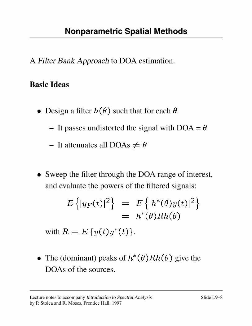
Nonparametric Spatial Methods
A Filter Bank Approach to DOA estimation.
Basic Ideas
� Design a filter h(�) such that for each �
– It passes undistorted the signal with DOA = �
– It attenuates all DOAs 6= �
� Sweep the filter through the DOA range of interest,
and evaluate the powers of the filtered signals:
EnjyF(t)j
2o
= Enjh�(�)y(t)j2
o= h�(�)Rh(�)
with R = E fy(t)y�(t)g.
� The (dominant) peaks of h�(�)Rh(�) give the
DOAs of the sources.
Lecture notes to accompany Introduction to Spectral Analysis Slide L9–8by P. Stoica and R. Moses, Prentice Hall, 1997
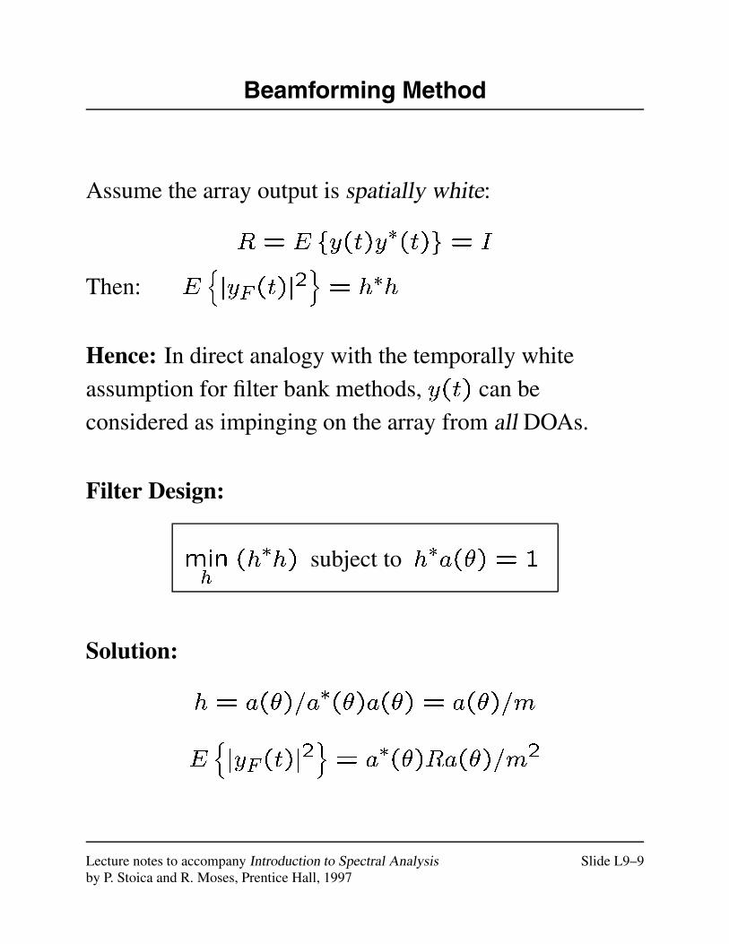
Beamforming Method
Assume the array output is spatially white:
R = E fy(t)y�(t)g = I
Then: EnjyF(t)j
2o= h�h
Hence: In direct analogy with the temporally white
assumption for filter bank methods, y(t) can be
considered as impinging on the array from all DOAs.
Filter Design:
minh
(h�h) subject to h�a(�) = 1
Solution:
h = a(�)=a�(�)a(�) = a(�)=m
EnjyF(t)j
2o= a�(�)Ra(�)=m2
Lecture notes to accompany Introduction to Spectral Analysis Slide L9–9by P. Stoica and R. Moses, Prentice Hall, 1997
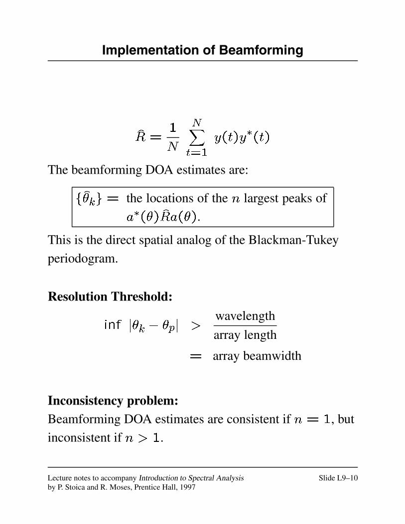
Implementation of Beamforming
R =1
N
NXt=1
y(t)y�(t)
The beamforming DOA estimates are:
f�kg= the locations of the n largest peaks of
a�(�)Ra(�).
This is the direct spatial analog of the Blackman-Tukey
periodogram.
Resolution Threshold:
inf j�k � �pj >wavelength
array length
= array beamwidth
Inconsistency problem:Beamforming DOA estimates are consistent if n= 1, but
inconsistent if n > 1.
Lecture notes to accompany Introduction to Spectral Analysis Slide L9–10by P. Stoica and R. Moses, Prentice Hall, 1997
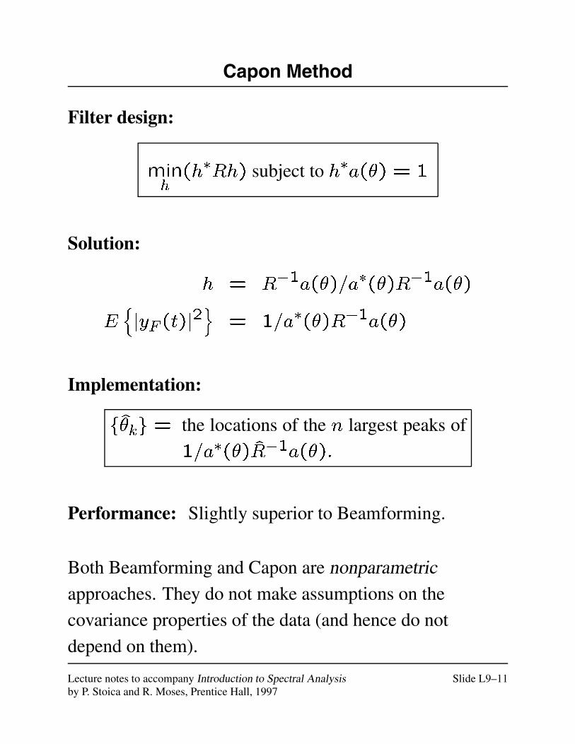
Capon Method
Filter design:
minh(h�Rh) subject to h�a(�) = 1
Solution:
h = R�1a(�)=a�(�)R�1a(�)
EnjyF(t)j
2o
= 1=a�(�)R�1a(�)
Implementation:
f�kg = the locations of the n largest peaks of
1=a�(�)R�1a(�):
Performance: Slightly superior to Beamforming.
Both Beamforming and Capon are nonparametricapproaches. They do not make assumptions on the
covariance properties of the data (and hence do not
depend on them).
Lecture notes to accompany Introduction to Spectral Analysis Slide L9–11by P. Stoica and R. Moses, Prentice Hall, 1997
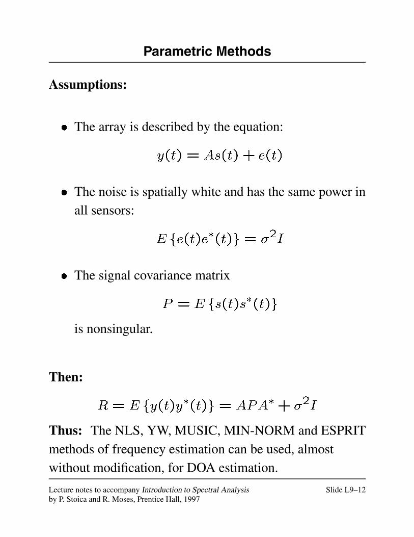
Parametric Methods
Assumptions:
� The array is described by the equation:
y(t) = As(t) + e(t)
� The noise is spatially white and has the same power inall sensors:
E fe(t)e�(t)g = �2I
� The signal covariance matrix
P = E fs(t)s�(t)g
is nonsingular.
Then:
R = E fy(t)y�(t)g = APA�+ �2I
Thus: The NLS, YW, MUSIC, MIN-NORM and ESPRITmethods of frequency estimation can be used, almostwithout modification, for DOA estimation.
Lecture notes to accompany Introduction to Spectral Analysis Slide L9–12by P. Stoica and R. Moses, Prentice Hall, 1997

Nonlinear Least Squares Method
minf�kg; fs(t)g
1
N
NXt=1
ky(t)�As(t)k2
| {z }f(�;s)
Minimizing f over s gives
s(t) = (A�A)�1A�y(t); t = 1; : : : ; N
Then
f(�; s) =1
N
NXt=1
k [I �A(A�A)�1A�]y(t)k2
=1
N
NXt=1
y�(t)[I �A(A�A)�1A�]y(t)
= trf[I �A(A�A)�1A�]Rg
Thus, f�kg= argmaxf�kg
trf[A(A�A)�1A�]Rg
For N = 1, this is precisely the form of the NLS method
of frequency estimation.
Lecture notes to accompany Introduction to Spectral Analysis Slide L9–13by P. Stoica and R. Moses, Prentice Hall, 1997
Nonlinear Least Squares Method
Properties of NLS:
� Performance: high
� Computational complexity: high
� Main drawback: need for multidimensional search.
Lecture notes to accompany Introduction to Spectral Analysis Slide L9–14by P. Stoica and R. Moses, Prentice Hall, 1997

Yule-Walker Method
y(t) =
"�y(t)~y(t)
#=
"�A~A
#s(t) +
"�e(t)~e(t)
#
Assume: E f�e(t)~e�(t)g = 0
Then:
�4= E f�y(t)~y�(t)g = �AP ~A� (M � L)
Also assume:
� M > n; L > n () m =M + L > 2n)
� rank( �A) = rank( ~A) = n
Then: rank(�) = n, and the SVD of � is
� = [U1|{z}n
U2|{z}M�n
]
"�n�n 00 0
# "V �1V �2
#g ng L�n
Properties: ~A�V2 = 0 V1 2 R( ~A)
Lecture notes to accompany Introduction to Spectral Analysis Slide L9–15by P. Stoica and R. Moses, Prentice Hall, 1997
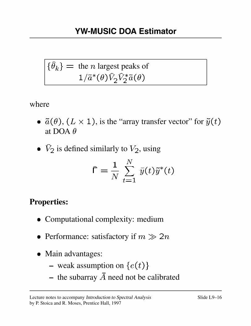
YW-MUSIC DOA Estimator
f�kg= the n largest peaks of
1=~a�(�)V2V�2~a(�)
where
� ~a(�), (L� 1), is the “array transfer vector” for ~y(t)at DOA �
� V2 is defined similarly to V2, using
� =1
N
NXt=1
�y(t)~y�(t)
Properties:
� Computational complexity: medium
� Performance: satisfactory if m� 2n
� Main advantages:
– weak assumption on fe(t)g
– the subarray �A need not be calibrated
Lecture notes to accompany Introduction to Spectral Analysis Slide L9–16by P. Stoica and R. Moses, Prentice Hall, 1997
MUSIC and Min-Norm Methods
Both MUSIC and Min-Norm methods for frequency
estimation apply with only minor modifications to the
DOA estimation problem.
� Spectral forms of MUSIC and Min-Norm can be used
for arbitrary arrays
� Root forms can be used only with ULAs
� MUSIC and Min-Norm break down if the source
signals are coherent; that is, if
rank(P) = rank(E fs(t)s�(t)g) < n
Modifications that apply in the coherent case exist.
Lecture notes to accompany Introduction to Spectral Analysis Slide L9–17by P. Stoica and R. Moses, Prentice Hall, 1997

ESPRIT Method
Assumption: The array is made from two identicalsubarrays separated by a known displacement vector.
Let
�m = # sensors in each subarray
A1 = [I�m 0]A (transfer matrix of subarray 1)
A2 = [0 I�m]A (transfer matrix of subarray 2)
Then A2 = A1D, where
D =
264 e
�i!c�(�1) 0. . .
0 e�i!c�(�n)
375
�(�) = the time delay from subarray 1 to
subarray 2 for a signal with DOA = �:
�(�) = d sin(�)=c
where d is the subarray separation and � is measured from
the perpendicular to the subarray displacement vector.
Lecture notes to accompany Introduction to Spectral Analysis Slide L9–18by P. Stoica and R. Moses, Prentice Hall, 1997
ESPRIT Method, con't
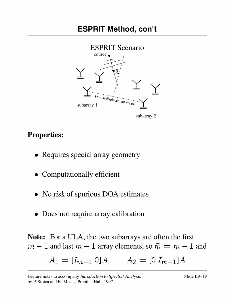
ESPRIT Scenario
subarray 1
subarray 2
source
θ
known displacement vector
Properties:
� Requires special array geometry
� Computationally efficient
� No risk of spurious DOA estimates
� Does not require array calibration
Note: For a ULA, the two subarrays are often the firstm�1 and last m�1 array elements, so �m = m�1 and
A1 = [Im�1 0]A; A2 = [0 Im�1]A
Lecture notes to accompany Introduction to Spectral Analysis Slide L9–19by P. Stoica and R. Moses, Prentice Hall, 1997