PHY331 Magnetism

Lecture 7

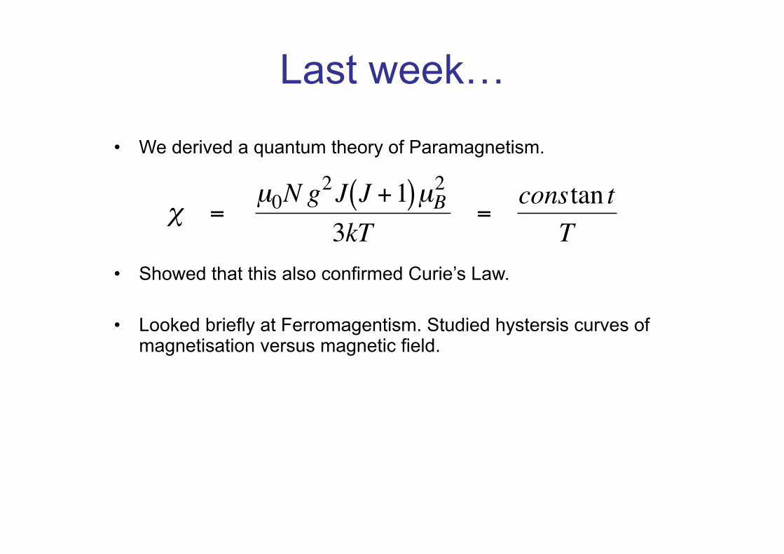
Last week…

•  We derived a quantum theory of Paramagnetism.

•  Showed that this also confirmed Curie’s Law.

•  Looked briefly at Ferromagentism. Studied hystersis curves of magnetisation versus magnetic field. €

χ =µ0N g

2J J +1( )µB2

3kT=

constan tT

This week…

•  Hysteresis curves •  The domain theory of Ferromagnetism. •  Motion of domain walls. •  Stabilization of domain walls and domain wall

thickness. •  Paramagnets vs ferromagnets.

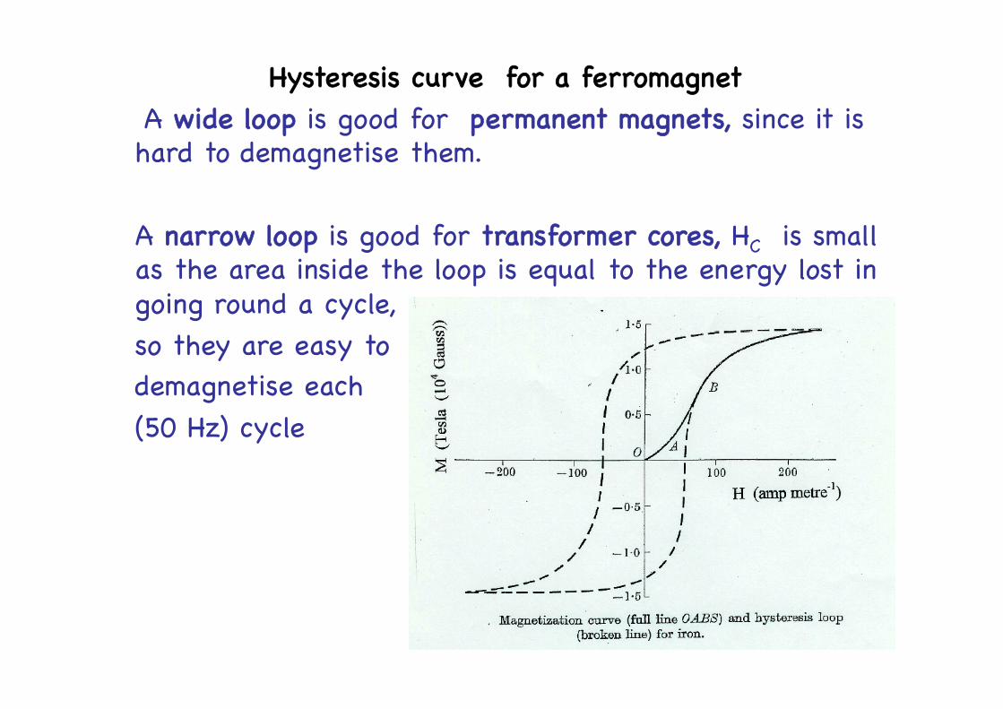
Hysteresis curve for a ferromagnet �" A wide loop is good for permanent magnets, since it is

hard to demagnetise them.�" �" A narrow loop is good for transformer cores, HC is small

as the area inside the loop is equal to the energy lost in going round a cycle, �

" so they are easy to �" demagnetise each �" (50 Hz) cycle

The domain theory of ferromagnetism

•  In a paramagnet, the increasing magnetisation M is due to the increasing alignment of the magnetic dipoles (in the - µ.B ≈ kT magnetic versus thermal “competition”)

•  For a ferromagnet, extremely large values of M can be created by the application of very small applied fields H

•  To produce such large M values by direct alignment of the magnetic moments would require applied fields about 1000 times greater

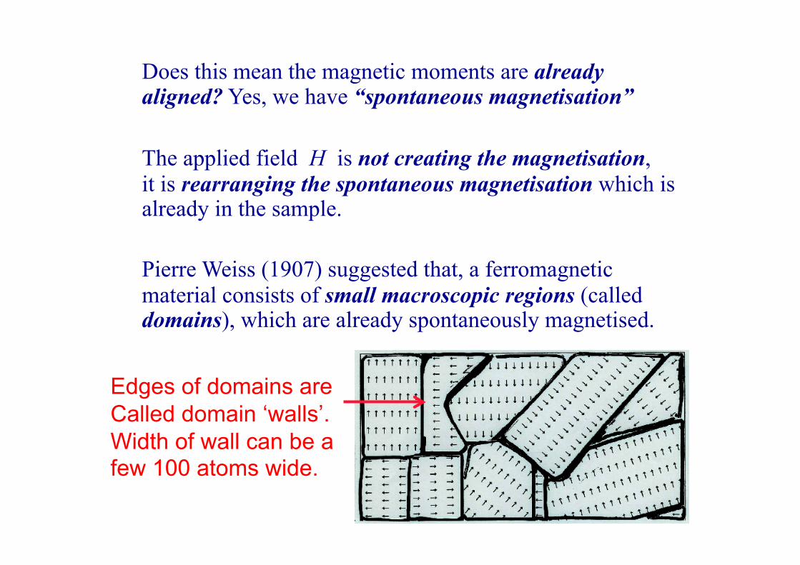
Does this mean the magnetic moments are already aligned? Yes, we have “spontaneous magnetisation”

The applied field H is not creating the magnetisation,

it is rearranging the spontaneous magnetisation which is already in the sample.

Pierre Weiss (1907) suggested that, a ferromagnetic

material consists of small macroscopic regions (called domains), which are already spontaneously magnetised.

Edges of domains are Called domain ‘walls’. Width of wall can be a few 100 atoms wide.

The magnitude of the magnetism M of a sample, is equal to the vector sum of the magnetisation

of the domains

The regions of spontaneous magnetisation obviously already exist and the external field H produces an overall magnetisation M by altering their distribution (size and distribution).

This model gives a qualitative description of the characteristic shape of the M v. H magnetisation curve

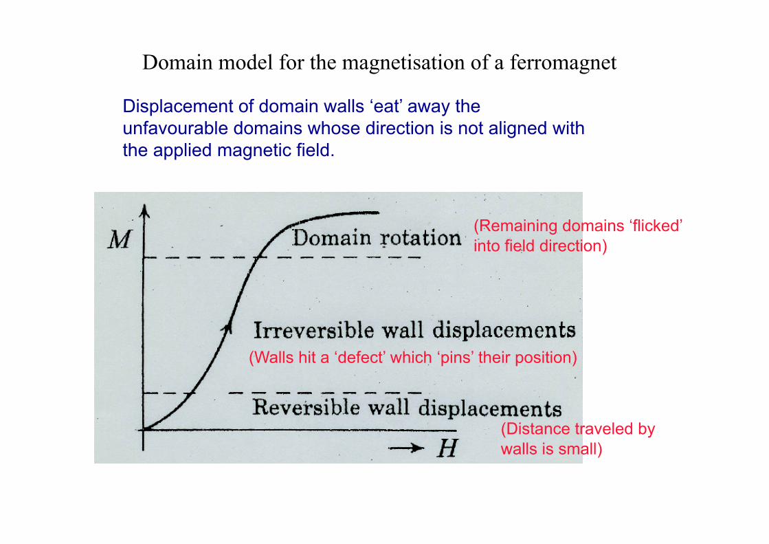
Domain model for the magnetisation of a ferromagnet

(Walls hit a ‘defect’ which ‘pins’ their position)

(Distance traveled by walls is small)

Displacement of domain walls ‘eat’ away the unfavourable domains whose direction is not aligned with the applied magnetic field.

(Remaining domains ‘flicked’ into field direction)

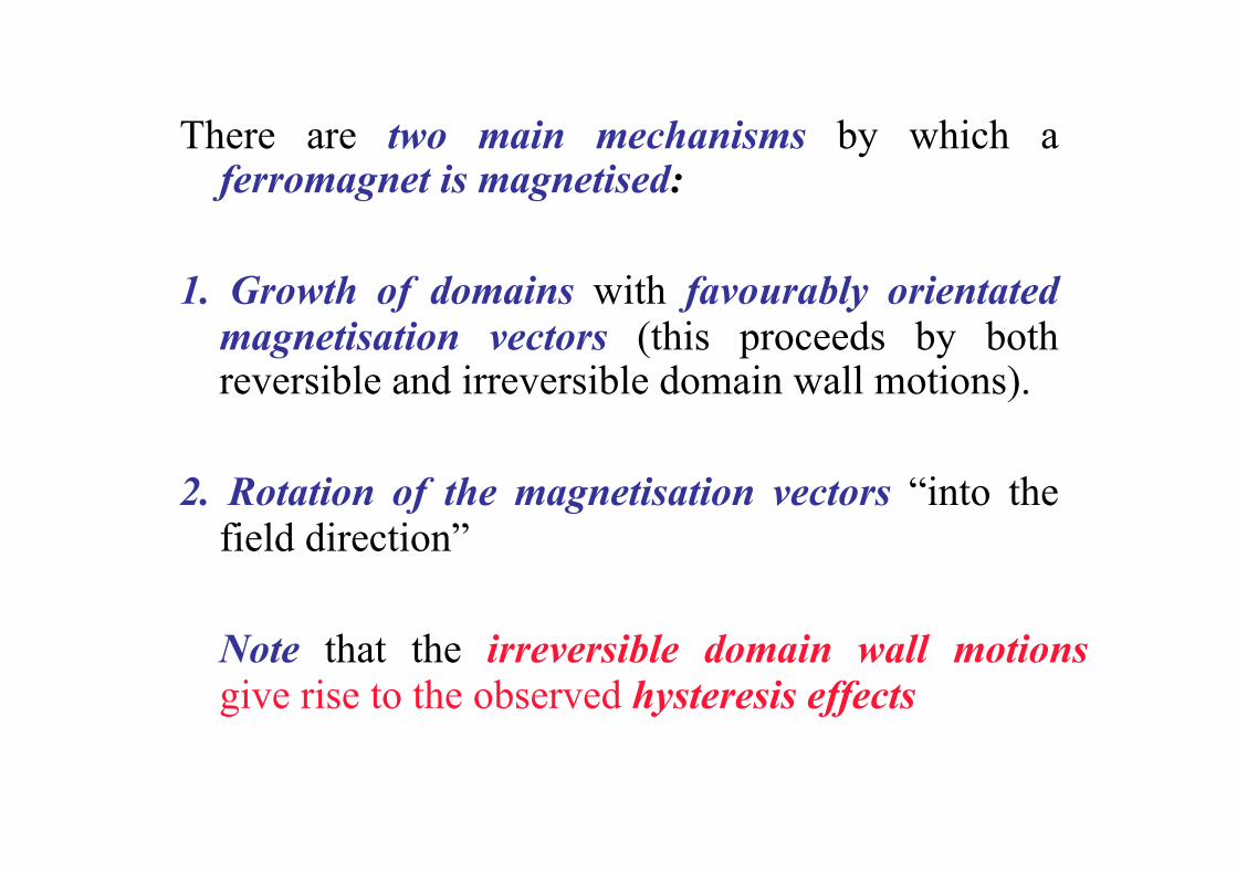
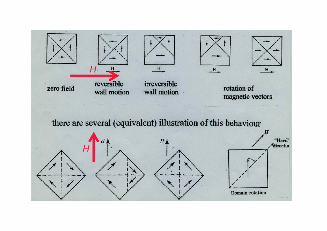
There are two main mechanisms by which a ferromagnet is magnetised:

1. Growth of domains with favourably orientated magnetisation vectors (this proceeds by both reversible and irreversible domain wall motions).

2. Rotation of the magnetisation vectors “into the field direction”

Note that the irreversible domain wall motions give rise to the observed hysteresis effects

H

H

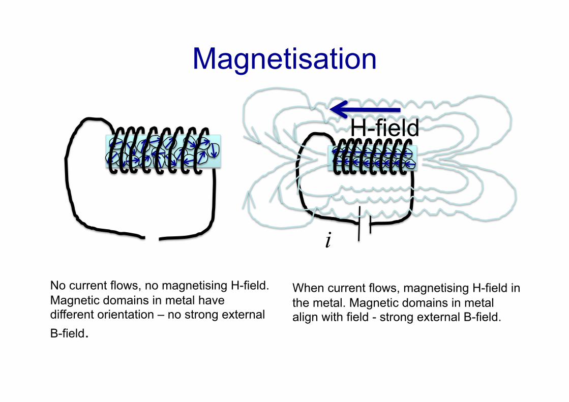
Magnetisation

No current flows, no magnetising H-field. Magnetic domains in metal have different orientation – no strong external B-field.

i

H-field

When current flows, magnetising H-field in the metal. Magnetic domains in metal align with field - strong external B-field.

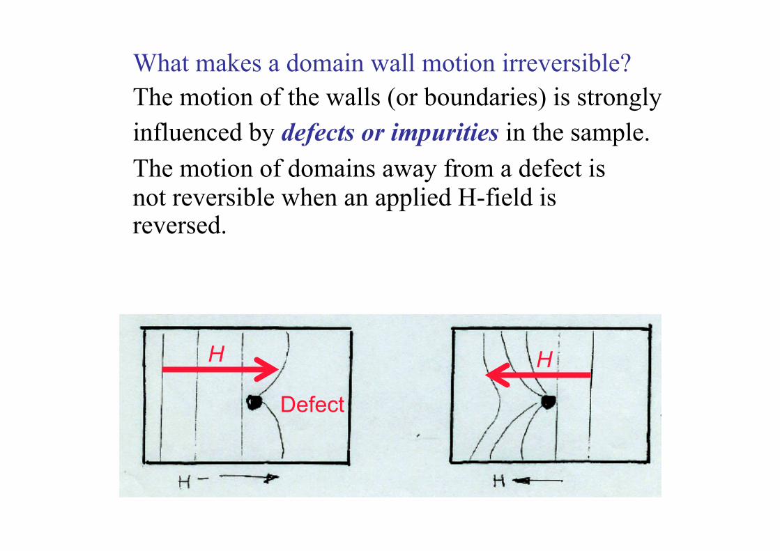
What makes a domain wall motion irreversible? The motion of the walls (or boundaries) is strongly influenced by defects or impurities in the sample. The motion of domains away from a defect is

not reversible when an applied H-field is reversed.

Defect

H H

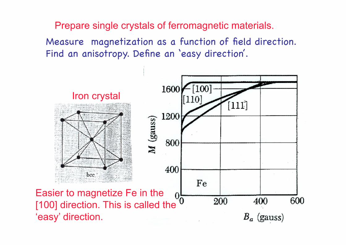
Prepare single crystals of ferromagnetic materials. Measure magnetization as a function of field direction.�Find an anisotropy. Define an ‘easy direction’.

Iron crystal

Easier to magnetize Fe in the [100] direction. This is called the ‘easy’ direction.

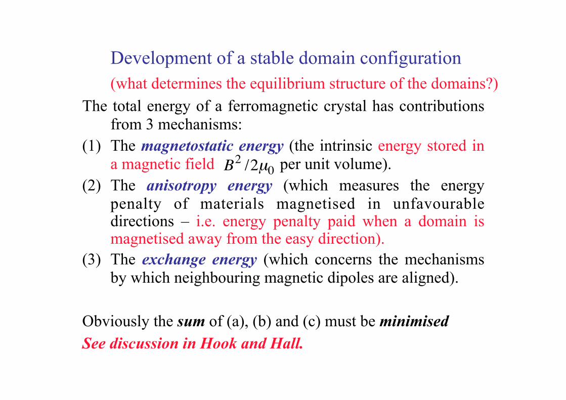
Development of a stable domain configuration (what determines the equilibrium structure of the domains?) The total energy of a ferromagnetic crystal has contributions

from 3 mechanisms: (1)  The magnetostatic energy (the intrinsic energy stored in

a magnetic field per unit volume). (2)  The anisotropy energy (which measures the energy

penalty of materials magnetised in unfavourable directions – i.e. energy penalty paid when a domain is magnetised away from the easy direction).

(3)  The exchange energy (which concerns the mechanisms by which neighbouring magnetic dipoles are aligned).

Obviously the sum of (a), (b) and (c) must be minimised See discussion in Hook and Hall.

€

B2 /2µ0

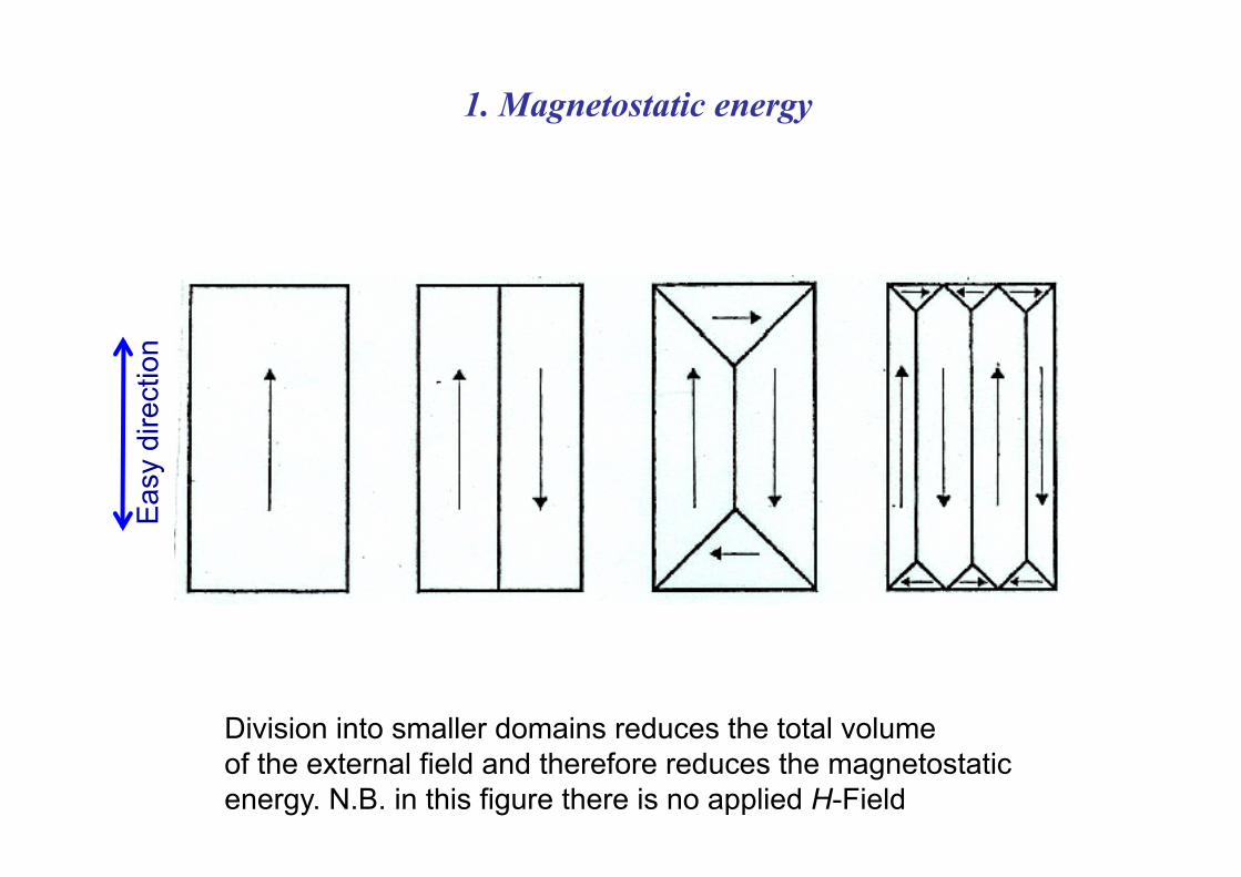
1. Magnetostatic energy

Division into smaller domains reduces the total volume of the external field and therefore reduces the magnetostatic energy. N.B. in this figure there is no applied H-Field

Eas

y di

rect

ion

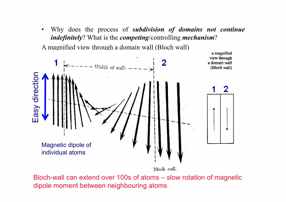
•  Why does the process of subdivision of domains not continue indefinitely? What is the competing/controlling mechanism?

A magnified view through a domain wall (Bloch wall)

Bloch-wall can extend over 100s of atoms – slow rotation of magnetic dipole moment between neighbouring atoms

Magnetic dipole of individual atoms

Eas

y di

rect

ion

‘Slow’ rotation of magnetic dipole across the wall occurs as large energy cost in having neighbouring atoms with different dipole orientation (exchange energy).

Within the domain wall, the majority of the magnetic dipole moments may be pointing out of the easy direction. This will then contribute to the anisotropy energy.

As domains get smaller, magnetostatic energy reduces,

however have more atoms found in the domain walls, and so the anisotropy energy grows.

Resulting balance between anisotropy, exchange and magnetostaic energies determine overall structure of domains and leads to establishment of an equilibrium structure.

What causes the alignment between neighbouring Magnetic dipole moments?

Several mechanisms have been proposed, including a quantum mechanical one based on the exchange of electrons between neighbouring atoms.

This is why the third contribution to the

magnetic energy. It has the generic name of “exchange energy”.

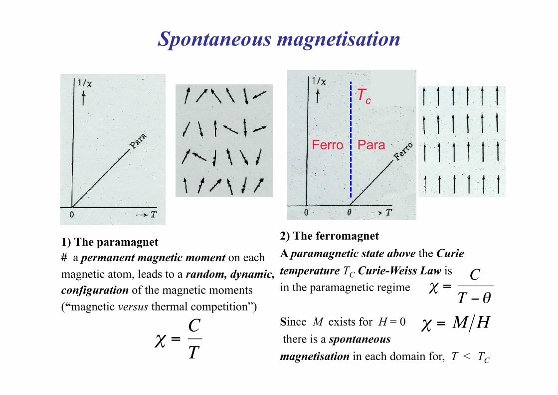
Spontaneous magnetisation

€

χ =CT

1) The paramagnet # a permanent magnetic moment on each magnetic atom, leads to a random, dynamic, configuration of the magnetic moments (“magnetic versus thermal competition”)

2) The ferromagnet A paramagnetic state above the Curie temperature TC Curie-Weiss Law is in the paramagnetic regime

Since M exists for H = 0 there is a spontaneous magnetisation in each domain for, T < TC

€

χ =C

T −θ

€

χ = M H

Ferro Para

Tc

Heating past Tc

•  If heat permanent magnet past Tc and then cool – ‘destroy’ domain structure. On cooling, have a random equilibrium structure of domains with no net magnetization.

•  Therefore heating a permanent magnet above Tc turns it back to a regular ferromagnetic solid.

Summary

•  Discussed domain theory of Ferromagnetism. •  Saw there is a motion of domain walls with

applied magnetic field. •  Stabilization of domain walls due to

competition between magnetostatic energy, anisptropy energy and exchange energy (see next week).

•  Forms domains having finite wall thickness.