MSE307 Engineering Alloys 2014-15 L7: Mechanical Behaviour of α + β Ti Alloys

D. Dyea

aRm G03b, Department of Materials, Imperial College London, London SW7 2AZ, UK. david.dye@imperial.ac.uk

In this lecture we examine microstructure - propertyrelationships and consider the mechanical behaviour of ti-tanium alloys, and begin a discussion that will span intolecture 7 on fatigue behaviour.

We have said previously that in titanium alloys, the keyis that on cooling from the β, there is little intragranularnucleation of α and so we see colonies of Widmanstatten αform. If we want a bimodal or equiaxed microstructure, wethen deform these plates high in the α+β phase field, andthen recrystallise them, also high in the α+ β phase field.This isn’t true recrystallisation where new grains nucleateand grow, rather it is the breakup and globularisation ofthe plates that already exist.

We’ve also looked and the α/β orientation relationshipand habit plane, and concluded that there are 12 variantsof α that can form from the β (6 distinct). Examining thehabit plane, we further found that there was was was oneprism slip system that could, relatively easily, be transmit-ted through an α/β colony structure, but that the othertwo easy slips would be restricted by the microstructure.

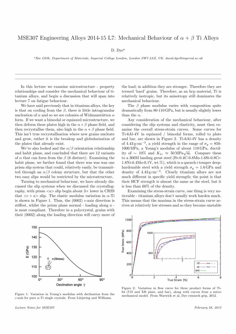
Turning to mechanical behaviour, we have already dis-cussed the slip systems when we discussed the crystallog-raphy, with prism <a> slip begin about 3× lower in CRSSthat <c + a> slip. The elastic modulus variation in α-Tiis shown in Figure 1. Thus, the (0002) c-axis direction isstiffest, whilst the prism plane normal - loading along a -is most compliant. Therefore in a polycrystal, grains withtheir (0002) along the loading direction will carry more of

Figure 1: Variation in Young’s modulus with declination from thec-axis for pure α-Ti single crystals. From Lutjering and Williams.

the load; in addition they are stronger. Therefore they aretermed ‘hard’ grains. Therefore, as an hcp material, Ti isrelatively isotropic, but its anisotropy still dominates themechanical behaviour.

The β phase modulus varies with composition quitedramatically from 80-110 GPa, but is usually slightly lowerthan the α.

Any consideration of the mechanical behaviour, afterconsidering the slip systems and elasticity, must then ex-amine the overall stress-strain curves. Some curves forTi-6Al-4V in equiaxed / bimodal forms, rolled to plateand bar, are shown in Figure 2. Ti-6Al-4V has a densityof 4.43 g cm−3, a yield strength in the range of σy = 850-1000 MPa, a Young’s modulus of about 110 GPa, ductil-ity of ∼ 10% and K1c ≈ 50 MPa

√m. Compare these

to a 300M landing great steel (Fe-0.4C-0.8Mn-1.6Si-0.8Cr-1.8Ni-0.4Mo-0.1V, wt.%), which is a quench+temper deep-hardenable steel with a yield strength σy = 1.6 GPa anddensity of 4.43 g cm−3. Clearly titanium alloys are notmuch different in specific yield strength; the point is thattheir HCF strength is almost the same as the steel, but itis less than 60% of the density.

Examining the stress-strain curve, one thing is very no-ticeable - titanium alloys don’t usually work harden much.This means that the maxima in the stress-strain curve ar-rives at relatively low stresses and so they become unstable

Figure 2: Variation in flow curve for three product forms of Ti-64 (UD and XR plate, and bar), along with curves from a micromechanical model. From Warwick et al, Dye research grip, 2012.

Lecture Notes for MSE307 February 28, 2015

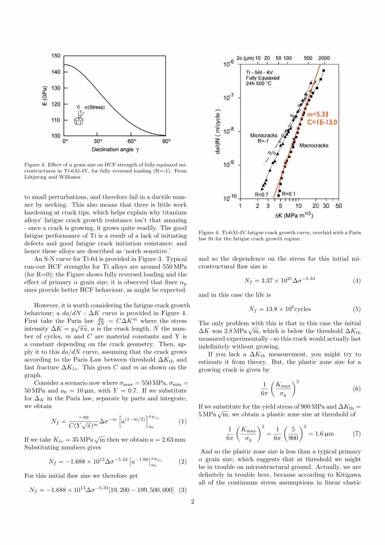
Figure 3: Effect of α grain size on HCF strength of fully equiaxed mi-crostructures in Ti-6Al-4V, for fully reversed loading (R=-1). FromLutjering and Williams.

to small perturbations, and therefore fail in a ductile man-ner by necking. This also means that there is little workhardening at crack tips, which helps explain why titaniumalloys’ fatigue crack growth resistance isn’t that amazing- once a crack is growing, it grows quite readily. The goodfatigue performance of Ti is a result of a lack of initiatingdefects and good fatigue crack initiation resistance; andhence these alloys are described as ‘notch sensitive.’

An S-N curve for Ti-64 is provided in Figure 3. Typicalrun-out HCF strengths for Ti alloys are around 550 MPa(for R=0); the Figure shows fully reversed loading and theeffect of primary α grain size; it is observed that finer αp

sizes provide better HCF behaviour, as might be expected.

However, it is worth considering the fatigue crack growthbehaviour; a da/dN - ∆K curve is provided in Figure 4.First take the Paris law da

dN = C∆Km where the stressintensity ∆K = y

√πa, a is the crack length, N the num-

ber of cycles, m and C are material constants and Y isa constant depending on the crack geometry. Then, ap-ply it to this da/dN curve, assuming that the crack growsaccording to the Paris Law between threshold ∆Kth andfast fracture ∆K1c. This gives C and m as shown on thegraph.

Consider a scenario now where σmax = 550 MPa, σmin =50 MPa and a0 = 10µm, with Y = 0.7. If we substitutefor ∆K in the Paris law, separate by parts and integrate,we obtain

Nf =−m

C(Y√π)m

∆σ−m[a(1−m/2)

]aK1c

a0

(1)

If we take K1c = 35 MPa√

m then we obtain a = 2.63 mm.Substituting numbers gives

Nf = −1.688× 1013∆σ−5.33[a−1.66

]aK1c

a0(2)

For this initial flaw size we therefore get

Nf = −1.688× 1013∆σ−5.33[19, 200− 199, 500, 000] (3)

Figure 4: Ti-6Al-4V fatigue crack growth curve, overlaid with a Parislaw fit for the fatigue crack growth regime.

and so the dependence on the stress for this initial mi-crostructural flaw size is

Nf = 3.37× 1021∆σ−5.33 (4)

and in this case the life is

Nf = 13.8× 106cycles (5)

The only problem with this is that in this case the initial∆K was 2.8 MPa

√m, which is below the threshold ∆Kth

measured experimentally - so this crack would actually lastindefinitely without growing.

If you lack a ∆Kth measurement, you might try toestimate it from theory. But, the plastic zone size for agrowing crack is given by

1

6π

(Kmax

σy

)2

(6)

If we substitute for the yield stress of 900 MPa and ∆Kth =5 MPa

√m, we obtain a plastic zone size at threshold of

1

6π

(Kmax

σy

)2

=1

6π

(5

900

)2

= 1.6µm (7)

And so the plastic zone size is less than a typical primaryα grain size, which suggests that at threshold we mightbe in trouble on microstructural ground. Actually, we aredefinitely in trouble here, because according to Kitigawaall of the continuum stress assumptions in linear elastic

2

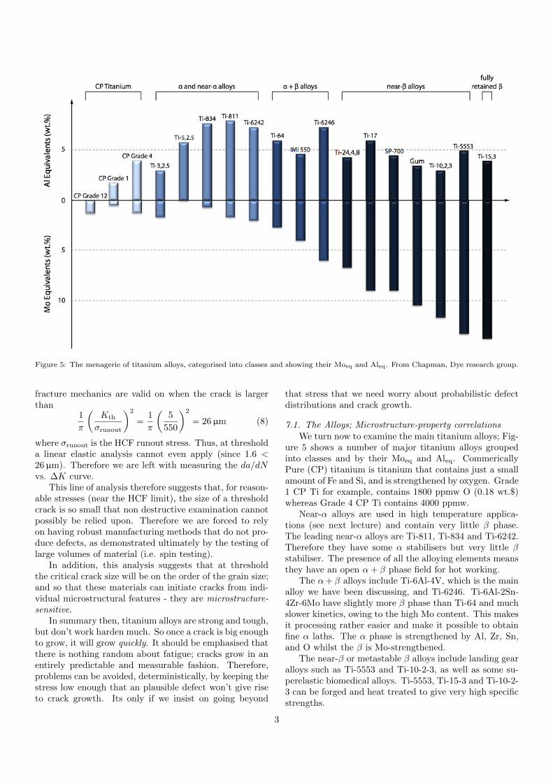
Figure 5: The menagerie of titanium alloys, categorised into classes and showing their Moeq and Aleq. From Chapman, Dye research group.

fracture mechanics are valid on when the crack is largerthan

1

π

(Kth

σrunout

)2

=1

π

(5

550

)2

= 26µm (8)

where σrunout is the HCF runout stress. Thus, at thresholda linear elastic analysis cannot even apply (since 1.6 <26µm). Therefore we are left with measuring the da/dNvs. ∆K curve.

This line of analysis therefore suggests that, for reason-able stresses (near the HCF limit), the size of a thresholdcrack is so small that non destructive examination cannotpossibly be relied upon. Therefore we are forced to relyon having robust manufacturing methods that do not pro-duce defects, as demonstrated ultimately by the testing oflarge volumes of material (i.e. spin testing).

In addition, this analysis suggests that at thresholdthe critical crack size will be on the order of the grain size;and so that these materials can initiate cracks from indi-vidual microstructural features - they are microstructure-sensitive.

In summary then, titanium alloys are strong and tough,but don’t work harden much. So once a crack is big enoughto grow, it will grow quickly. It should be emphasised thatthere is nothing random about fatigue; cracks grow in anentirely predictable and measurable fashion. Therefore,problems can be avoided, deterministically, by keeping thestress low enough that an plausible defect won’t give riseto crack growth. Its only if we insist on going beyond

that stress that we need worry about probabilistic defectdistributions and crack growth.

7.1. The Alloys; Microstructure-property correlationsWe turn now to examine the main titanium alloys; Fig-

ure 5 shows a number of major titanium alloys groupedinto classes and by their Moeq and Aleq. CommericallyPure (CP) titanium is titanium that contains just a smallamount of Fe and Si, and is strengthened by oxygen. Grade1 CP Ti for example, contains 1800 ppmw O (0.18 wt.$)whereas Grade 4 CP Ti contains 4000 ppmw.

Near-α alloys are used in high temperature applica-tions (see next lecture) and contain very little β phase.The leading near-α alloys are Ti-811, Ti-834 and Ti-6242.Therefore they have some α stabilisers but very little βstabiliser. The presence of all the alloying elements meansthey have an open α+ β phase field for hot working.

The α+ β alloys include Ti-6Al-4V, which is the mainalloy we have been discussing, and Ti-6246. Ti-6Al-2Sn-4Zr-6Mo have slightly more β phase than Ti-64 and muchslower kinetics, owing to the high Mo content. This makesit processing rather easier and make it possible to obtainfine α laths. The α phase is strengthened by Al, Zr, Sn,and O whilst the β is Mo-strengthened.

The near-β or metastable β alloys include landing gearalloys such as Ti-5553 and Ti-10-2-3, as well as some su-perelastic biomedical alloys. Ti-5553, Ti-15-3 and Ti-10-2-3 can be forged and heat treated to give very high specificstrengths.

3

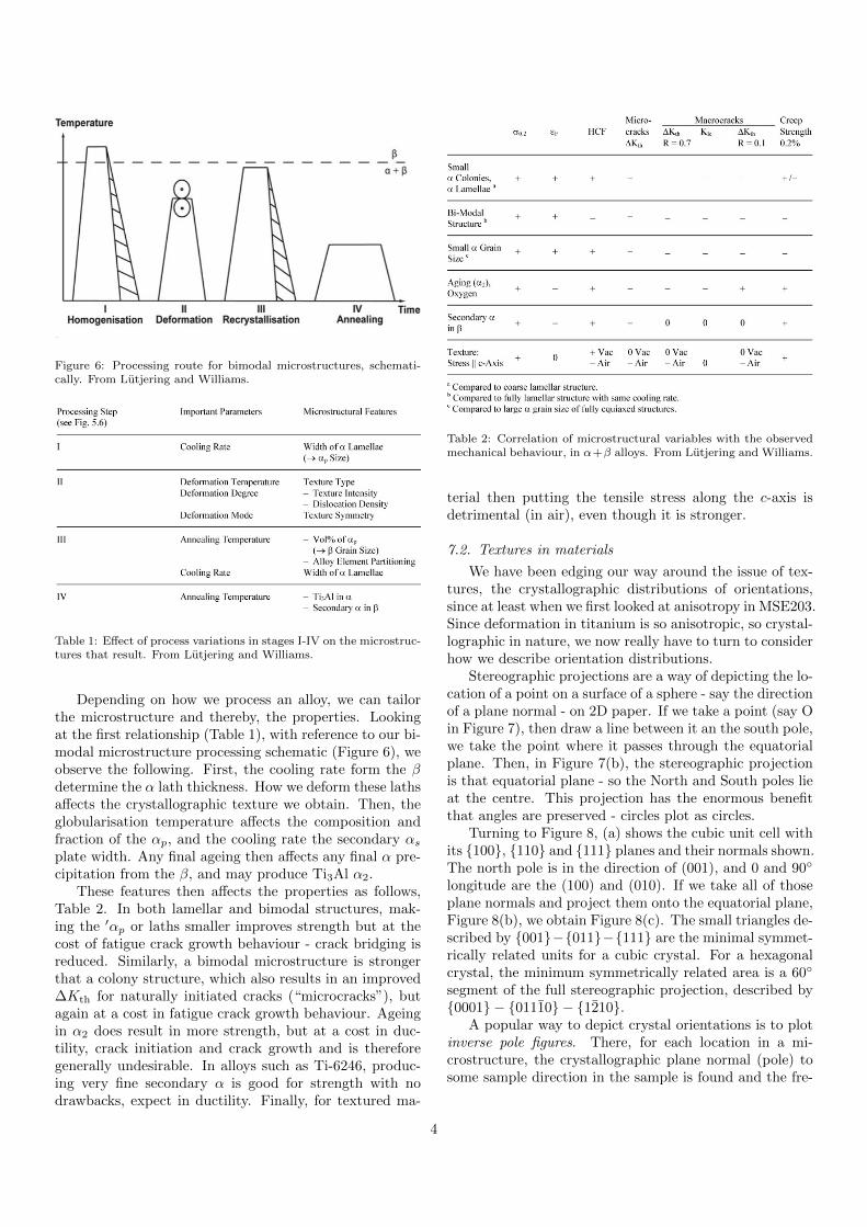
Figure 6: Processing route for bimodal microstructures, schemati-cally. From Lutjering and Williams.

Table 1: Effect of process variations in stages I-IV on the microstruc-tures that result. From Lutjering and Williams.

Depending on how we process an alloy, we can tailorthe microstructure and thereby, the properties. Lookingat the first relationship (Table 1), with reference to our bi-modal microstructure processing schematic (Figure 6), weobserve the following. First, the cooling rate form the βdetermine the α lath thickness. How we deform these lathsaffects the crystallographic texture we obtain. Then, theglobularisation temperature affects the composition andfraction of the αp, and the cooling rate the secondary αs

plate width. Any final ageing then affects any final α pre-cipitation from the β, and may produce Ti3Al α2.

These features then affects the properties as follows,Table 2. In both lamellar and bimodal structures, mak-ing the ′αp or laths smaller improves strength but at thecost of fatigue crack growth behaviour - crack bridging isreduced. Similarly, a bimodal microstructure is strongerthat a colony structure, which also results in an improved∆Kth for naturally initiated cracks (“microcracks”), butagain at a cost in fatigue crack growth behaviour. Ageingin α2 does result in more strength, but at a cost in duc-tility, crack initiation and crack growth and is thereforegenerally undesirable. In alloys such as Ti-6246, produc-ing very fine secondary α is good for strength with nodrawbacks, expect in ductility. Finally, for textured ma-

Table 2: Correlation of microstructural variables with the observedmechanical behaviour, in α+β alloys. From Lutjering and Williams.

terial then putting the tensile stress along the c-axis isdetrimental (in air), even though it is stronger.

7.2. Textures in materials

We have been edging our way around the issue of tex-tures, the crystallographic distributions of orientations,since at least when we first looked at anisotropy in MSE203.Since deformation in titanium is so anisotropic, so crystal-lographic in nature, we now really have to turn to considerhow we describe orientation distributions.

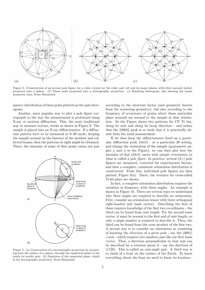
Stereographic projections are a way of depicting the lo-cation of a point on a surface of a sphere - say the directionof a plane normal - on 2D paper. If we take a point (say Oin Figure 7), then draw a line between it an the south pole,we take the point where it passes through the equatorialplane. Then, in Figure 7(b), the stereographic projectionis that equatorial plane - so the North and South poles lieat the centre. This projection has the enormous benefitthat angles are preserved - circles plot as circles.

Turning to Figure 8, (a) shows the cubic unit cell withits {100}, {110} and {111} planes and their normals shown.The north pole is in the direction of (001), and 0 and 90◦

longitude are the (100) and (010). If we take all of thoseplane normals and project them onto the equatorial plane,Figure 8(b), we obtain Figure 8(c). The small triangles de-scribed by {001}−{011}−{111} are the minimal symmet-rically related units for a cubic crystal. For a hexagonalcrystal, the minimum symmetrically related area is a 60◦

segment of the full stereographic projection, described by{0001} − {01110} − {1210}.

A popular way to depict crystal orientations is to plotinverse pole figures. There, for each location in a mi-crostructure, the crystallographic plane normal (pole) tosome sample direction in the sample is found and the fre-

4

(a) (b) (c)

Figure 8: (Construction of an inverse pole figure, for a cubic crystal (a) the cubic unit cell and its major planes, with their normals (poles)projected onto a sphere. (b) Those poles projected onto a stereographic projection. (c) Resulting stereogram, also showing the majorsymmetry axes. From Hammond.

quency distribution of these poles plotted on the unit stere-ogram.

Another, more popular way to plot a pole figure cor-responds to the way the measurement is performed usingX-ray or neutron diffraction. This, the most traditionalway to measure texture, works as shown in Figure 9. Thesample is placed into an X-ray diffractometer. If a diffrac-tion pattern were to be measured in θ–2θ mode, keepingthe sample normal on the bisector of the incident and col-lected beams, then the patterns at right might be obtained.There, the intensity of some of thee peaks varies not just

Figure 7: (a) Construction of a stereographic projection by project-ing from the surface of a sphere, through the equatorial plane to thesouth (or north) pole. (b) Depiction of the equatorial plane, whichis the stereographic projection. From Hammond

according to the structure factor (and geometric factorsfrom the scattering geometry), but also according to thefrequency of occurrence of grains where those particularplane normals are normal to the sample in that orienta-tion. So the Figure shows two patterns for CP Ti bar,along its axis and along its hoop direction - and noticethat the {0002} peak is so weak that it is practically ab-sent form the axial measurement.

If we then keep the diffractometer fixed on a partic-ular diffraction peak {hkil} - at a particular 2θ setting,and change the orientation of the sample (goniometer an-gles χ and φ in the Figure), we can then plot how theintensity of that {hkil} varies with sample orientation, inwhat is called a pole figure. In practice, several (3+) polefigures are measured, corrected for experimental factors,and then a complete, consistent orientation distribution isconstructed. From this, individual pole figures are thenplotted, Figure 9(a). There, the textures for cross-rolledTi-64 plate are shown.

In fact, a complete orientation distribution requires thevariation in frequency with three angles. An example isshown in Figure 10. There are several ways to understandwhy three angles are required to describe an orientation.First, consider an orientation tensor with three orthogonalright-handed unit basis vectors. Describing the first ofthese requires knowledge of the first two co-ordinates - thethird can be found from unit length. For the second basisvector, it must be normal to the first and of unit length, soonly a single number is required to describe it. Then, thethird can be found form the cross product of the first two.A second way is to consider an orientation as consistingof knowing the direction of a given pole - say the (0001)c-axis - which requires two numbers just iike our first basisvector. Then, a direction perpendicular to that axis canbe described by a rotation about it - say the direction of(1120). This is called an axis-angle pair. A third way isto think of a boat on the surface of the Earth. To knoweverything about the boat we need to know its location -

5

Figure 9: (left) Example of two pole figures, for the {0002} and {1010}, measured for cross-rolled Ti-6-4 plate using lab. X-ray diffraction(Warwick, red=most intense, green = 1× random, blue=least intense). (middle) setup of a pole figure measurement on an X-ray diffractometer,from Hammond. (right) diffraction patterns for two directions in CP Ti bar material (Warwick).

latitude and longitude - and its direction - the way it ispointing.

Therefore, a single pole figure can’t describe an orien-tation distribution fully - it only describes the frequencyfor the particular plane normal measured. Thus, severalpole figures are measured and combined mathematically toget the complete orientation distribution. But, for mosthuman purposes it is easier to examine pole figures whenwe are thinking about textures, because we can readilyrelate them to directions in crystals.

The Bunge description of orientations uses three Eulerangles, Figure 11. The first, ψ1, describes a rotation aboutZ, rotatingX and Y as shown. Then, we rotate by φ aboutthe new (dotted) X-axis, which rotate Z to Z ′. The final,third, rotation is also about Z ′, by an angle ψ2, to obtainthe final X ′ and Y ′ axes (leaving Z ′ alone).

Figure 10: Example of a complete orientation distribution function(ODF), in β annealed Ti-6Al-4V plate (Warwick). A pole figure onlyshows frequency vs two angles, whereas the full ODF requires threeangles, produced by combining 3 or more pole figures.

A second way to measure textures is in the SEM. There,if we tilt the sample by 70◦ to the incident beam and ex-amine the electron scattering at 90◦ to the incident beam,we observe channelling patterns. These Kikuchi bands,which intersects at poles, correspond to electrons chan-nelling down the planes of the crystal. These bands canbe fitted to a model of the crystal structure and the (com-plete) crystal orientation obtained. We can then find thedirection of the crystallographic plane normal to a par-ticular sample direction - the location in the inverse polefigure (IPF) - and assign a colour according to that IPF.Then , we can plot the spatial variation in these colours,obtaining an ‘orientation-coloured microstructural map,’Figure 12. Often, the IPF is with respect to the sample

Figure 11: Rotation of a set of orthonormal basis vectors (XYZ, red)by a set of Bunge Euler angles (ψ1 about Z, then φ about X, then ψ2

about Z′) to a new orientation. From Warwick, PhD thesis, ImperialCollege, 2012.

6

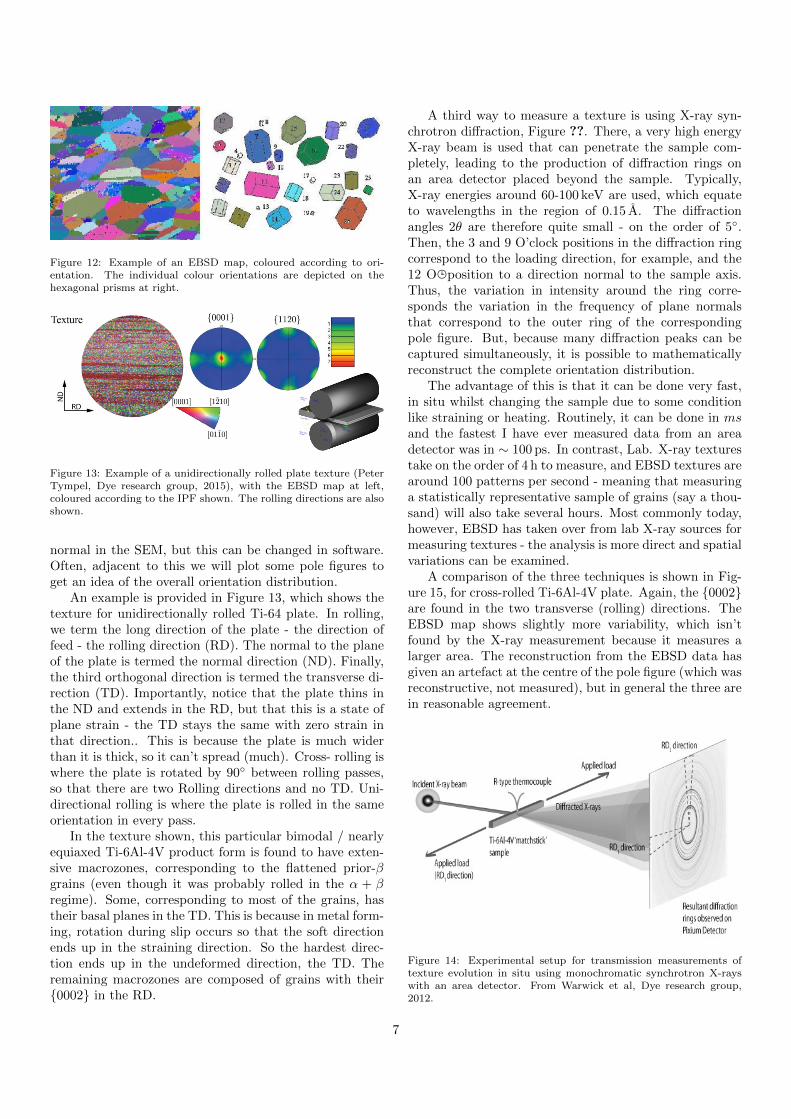
Figure 12: Example of an EBSD map, coloured according to ori-entation. The individual colour orientations are depicted on thehexagonal prisms at right.

Figure 13: Example of a unidirectionally rolled plate texture (PeterTympel, Dye research group, 2015), with the EBSD map at left,coloured according to the IPF shown. The rolling directions are alsoshown.

normal in the SEM, but this can be changed in software.Often, adjacent to this we will plot some pole figures toget an idea of the overall orientation distribution.

An example is provided in Figure 13, which shows thetexture for unidirectionally rolled Ti-64 plate. In rolling,we term the long direction of the plate - the direction offeed - the rolling direction (RD). The normal to the planeof the plate is termed the normal direction (ND). Finally,the third orthogonal direction is termed the transverse di-rection (TD). Importantly, notice that the plate thins inthe ND and extends in the RD, but that this is a state ofplane strain - the TD stays the same with zero strain inthat direction.. This is because the plate is much widerthan it is thick, so it can’t spread (much). Cross- rolling iswhere the plate is rotated by 90◦ between rolling passes,so that there are two Rolling directions and no TD. Uni-directional rolling is where the plate is rolled in the sameorientation in every pass.

In the texture shown, this particular bimodal / nearlyequiaxed Ti-6Al-4V product form is found to have exten-sive macrozones, corresponding to the flattened prior-βgrains (even though it was probably rolled in the α + βregime). Some, corresponding to most of the grains, hastheir basal planes in the TD. This is because in metal form-ing, rotation during slip occurs so that the soft directionends up in the straining direction. So the hardest direc-tion ends up in the undeformed direction, the TD. Theremaining macrozones are composed of grains with their{0002} in the RD.

A third way to measure a texture is using X-ray syn-chrotron diffraction, Figure ??. There, a very high energyX-ray beam is used that can penetrate the sample com-pletely, leading to the production of diffraction rings onan area detector placed beyond the sample. Typically,X-ray energies around 60-100 keV are used, which equateto wavelengths in the region of 0.15 A. The diffractionangles 2θ are therefore quite small - on the order of 5◦.Then, the 3 and 9 O’clock positions in the diffraction ringcorrespond to the loading direction, for example, and the12 O�position to a direction normal to the sample axis.Thus, the variation in intensity around the ring corre-sponds the variation in the frequency of plane normalsthat correspond to the outer ring of the correspondingpole figure. But, because many diffraction peaks can becaptured simultaneously, it is possible to mathematicallyreconstruct the complete orientation distribution.

The advantage of this is that it can be done very fast,in situ whilst changing the sample due to some conditionlike straining or heating. Routinely, it can be done in msand the fastest I have ever measured data from an areadetector was in ∼ 100 ps. In contrast, Lab. X-ray texturestake on the order of 4 h to measure, and EBSD textures arearound 100 patterns per second - meaning that measuringa statistically representative sample of grains (say a thou-sand) will also take several hours. Most commonly today,however, EBSD has taken over from lab X-ray sources formeasuring textures - the analysis is more direct and spatialvariations can be examined.

A comparison of the three techniques is shown in Fig-ure 15, for cross-rolled Ti-6Al-4V plate. Again, the {0002}are found in the two transverse (rolling) directions. TheEBSD map shows slightly more variability, which isn’tfound by the X-ray measurement because it measures alarger area. The reconstruction from the EBSD data hasgiven an artefact at the centre of the pole figure (which wasreconstructive, not measured), but in general the three arein reasonable agreement.

Figure 14: Experimental setup for transmission measurements oftexture evolution in situ using monochromatic synchrotron X-rayswith an area detector. From Warwick et al, Dye research group,2012.

7

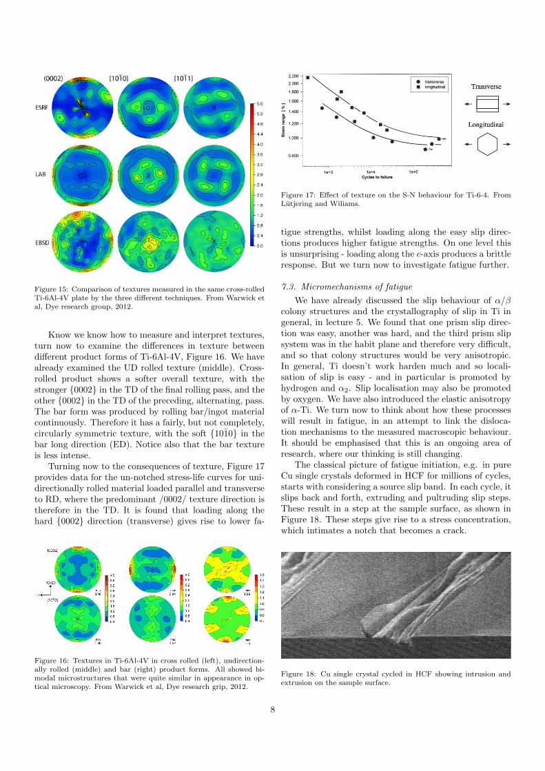
Figure 15: Comparison of textures measured in the same cross-rolledTi-6Al-4V plate by the three different techniques. From Warwick etal, Dye research group, 2012.

Know we know how to measure and interpret textures,turn now to examine the differences in texture betweendifferent product forms of Ti-6Al-4V, Figure 16. We havealready examined the UD rolled texture (middle). Cross-rolled product shows a softer overall texture, with thestronger {0002} in the TD of the final rolling pass, and theother {0002} in the TD of the preceding, alternating, pass.The bar form was produced by rolling bar/ingot materialcontinuously. Therefore it has a fairly, but not completely,circularly symmetric texture, with the soft {1010} in thebar long direction (ED). Notice also that the bar textureis less intense.

Turning now to the consequences of texture, Figure 17provides data for the un-notched stress-life curves for uni-directionally rolled material loaded parallel and transverseto RD, where the predominant /0002/ texture direction istherefore in the TD. It is found that loading along thehard {0002} direction (transverse) gives rise to lower fa-

Figure 16: Textures in Ti-6Al-4V in cross rolled (left), undirection-ally rolled (middle) and bar (right) product forms. All showed bi-modal microstructures that were quite similar in appearance in op-tical microscopy. From Warwick et al, Dye research grip, 2012.

Figure 17: Effect of texture on the S-N behaviour for Ti-6-4. FromLutjering and Wiliams.

tigue strengths, whilst loading along the easy slip direc-tions produces higher fatigue strengths. On one level thisis unsurprising - loading along the c-axis produces a brittleresponse. But we turn now to investigate fatigue further.

7.3. Micromechanisms of fatigue

We have already discussed the slip behaviour of α/βcolony structures and the crystallography of slip in Ti ingeneral, in lecture 5. We found that one prism slip direc-tion was easy, another was hard, and the third prism slipsystem was in the habit plane and therefore very difficult,and so that colony structures would be very anisotropic.In general, Ti doesn’t work harden much and so locali-sation of slip is easy - and in particular is promoted byhydrogen and α2. Slip localisation may also be promotedby oxygen. We have also introduced the elastic anisotropyof α-Ti. We turn now to think about how these processeswill result in fatigue, in an attempt to link the disloca-tion mechanisms to the measured macroscopic behaviour.It should be emphasised that this is an ongoing area ofresearch, where our thinking is still changing.

The classical picture of fatigue initiation, e.g. in pureCu single crystals deformed in HCF for millions of cycles,starts with considering a source slip band. In each cycle, itslips back and forth, extruding and pultruding slip steps.These result in a step at the sample surface, as shown inFigure 18. These steps give rise to a stress concentration,which intimates a notch that becomes a crack.

Figure 18: Cu single crystal cycled in HCF showing intrusion andextrusion on the sample surface.

8

Cold dwell fatigue is a particular phenomenon of in-terest in the titanium industry. In this phenomenon, 10×reductions in cyclic life are observed when a load hold ofseveral minutes is introduced at the peak load during afatigue cycle at ambient temperature.

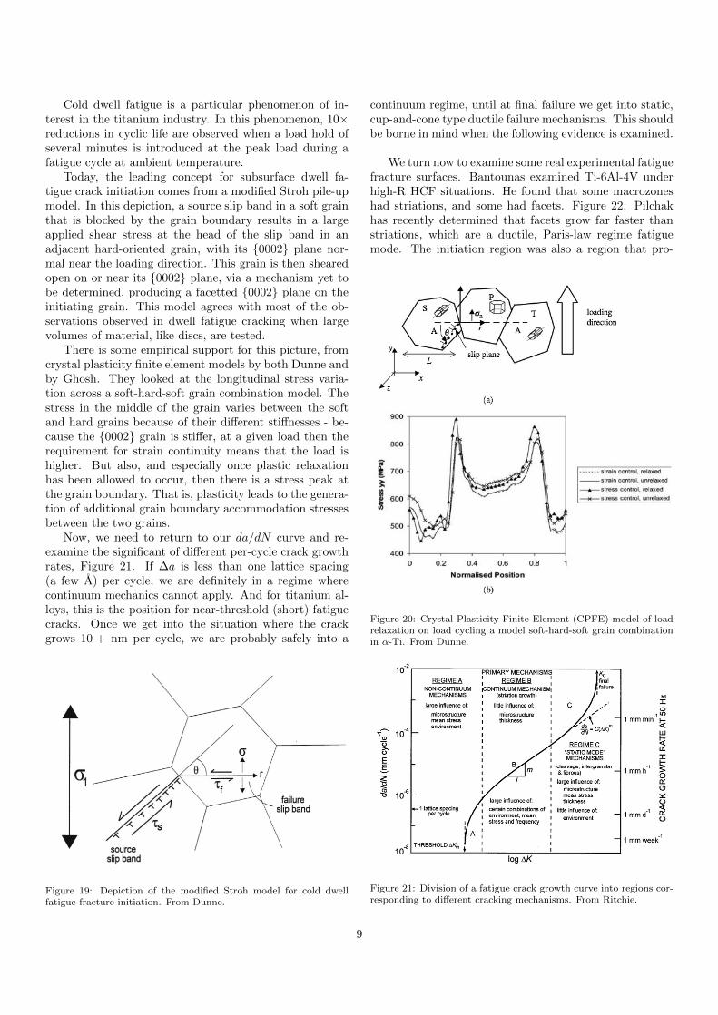
Today, the leading concept for subsurface dwell fa-tigue crack initiation comes from a modified Stroh pile-upmodel. In this depiction, a source slip band in a soft grainthat is blocked by the grain boundary results in a largeapplied shear stress at the head of the slip band in anadjacent hard-oriented grain, with its {0002} plane nor-mal near the loading direction. This grain is then shearedopen on or near its {0002} plane, via a mechanism yet tobe determined, producing a facetted {0002} plane on theinitiating grain. This model agrees with most of the ob-servations observed in dwell fatigue cracking when largevolumes of material, like discs, are tested.

There is some empirical support for this picture, fromcrystal plasticity finite element models by both Dunne andby Ghosh. They looked at the longitudinal stress varia-tion across a soft-hard-soft grain combination model. Thestress in the middle of the grain varies between the softand hard grains because of their different stiffnesses - be-cause the {0002} grain is stiffer, at a given load then therequirement for strain continuity means that the load ishigher. But also, and especially once plastic relaxationhas been allowed to occur, then there is a stress peak atthe grain boundary. That is, plasticity leads to the genera-tion of additional grain boundary accommodation stressesbetween the two grains.

Now, we need to return to our da/dN curve and re-examine the significant of different per-cycle crack growthrates, Figure 21. If ∆a is less than one lattice spacing(a few A) per cycle, we are definitely in a regime wherecontinuum mechanics cannot apply. And for titanium al-loys, this is the position for near-threshold (short) fatiguecracks. Once we get into the situation where the crackgrows 10 + nm per cycle, we are probably safely into a

Figure 19: Depiction of the modified Stroh model for cold dwellfatigue fracture initiation. From Dunne.

continuum regime, until at final failure we get into static,cup-and-cone type ductile failure mechanisms. This shouldbe borne in mind when the following evidence is examined.

We turn now to examine some real experimental fatiguefracture surfaces. Bantounas examined Ti-6Al-4V underhigh-R HCF situations. He found that some macrozoneshad striations, and some had facets. Figure 22. Pilchakhas recently determined that facets grow far faster thanstriations, which are a ductile, Paris-law regime fatiguemode. The initiation region was also a region that pro-

Figure 20: Crystal Plasticity Finite Element (CPFE) model of loadrelaxation on load cycling a model soft-hard-soft grain combinationin α-Ti. From Dunne.

Figure 21: Division of a fatigue crack growth curve into regions cor-responding to different cracking mechanisms. From Ritchie.

9

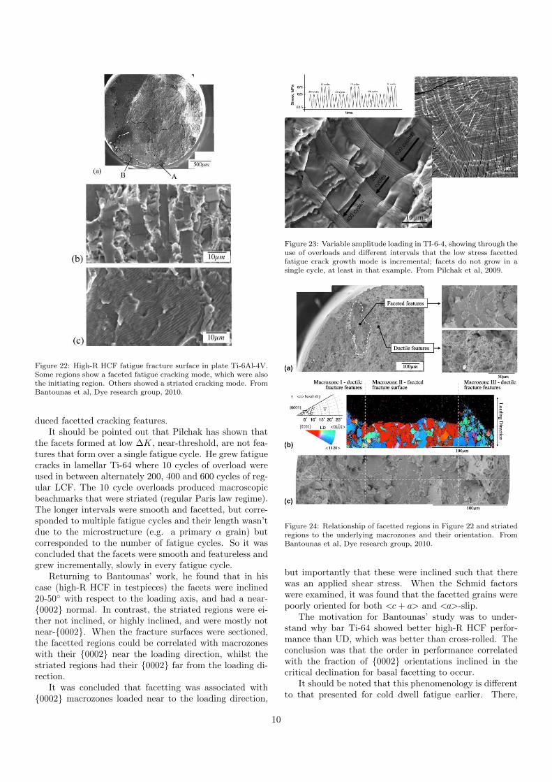
Figure 22: High-R HCF fatigue fracture surface in plate Ti-6Al-4V.Some regions show a faceted fatigue cracking mode, which were alsothe initiating region. Others showed a striated cracking mode. FromBantounas et al, Dye research group, 2010.

duced facetted cracking features.It should be pointed out that Pilchak has shown that

the facets formed at low ∆K, near-threshold, are not fea-tures that form over a single fatigue cycle. He grew fatiguecracks in lamellar Ti-64 where 10 cycles of overload wereused in between alternately 200, 400 and 600 cycles of reg-ular LCF. The 10 cycle overloads produced macroscopicbeachmarks that were striated (regular Paris law regime).The longer intervals were smooth and facetted, but corre-sponded to multiple fatigue cycles and their length wasn’tdue to the microstructure (e.g. a primary α grain) butcorresponded to the number of fatigue cycles. So it wasconcluded that the facets were smooth and featureless andgrew incrementally, slowly in every fatigue cycle.

Returning to Bantounas’ work, he found that in hiscase (high-R HCF in testpieces) the facets were inclined20-50◦ with respect to the loading axis, and had a near-{0002} normal. In contrast, the striated regions were ei-ther not inclined, or highly inclined, and were mostly notnear-{0002}. When the fracture surfaces were sectioned,the facetted regions could be correlated with macrozoneswith their {0002} near the loading direction, whilst thestriated regions had their {0002} far from the loading di-rection.

It was concluded that facetting was associated with{0002} macrozones loaded near to the loading direction,

Figure 23: Variable amplitude loading in TI-6-4, showing through theuse of overloads and different intervals that the low stress facettedfatigue crack growth mode is incremental; facets do not grow in asingle cycle, at least in that example. From Pilchak et al, 2009.

Figure 24: Relationship of facetted regions in Figure 22 and striatedregions to the underlying macrozones and their orientation. FromBantounas et al, Dye research group, 2010.

but importantly that these were inclined such that therewas an applied shear stress. When the Schmid factorswere examined, it was found that the facetted grains werepoorly oriented for both <c+ a> and <a>-slip.

The motivation for Bantounas’ study was to under-stand why bar Ti-64 showed better high-R HCF perfor-mance than UD, which was better than cross-rolled. Theconclusion was that the order in performance correlatedwith the fraction of {0002} orientations inclined in thecritical declination for basal facetting to occur.

It should be noted that this phenomenology is differentto that presented for cold dwell fatigue earlier. There,

10

the dwell facets usually have their plane normal along theloading direction, whilst for high-R HCF they are inclined.But, in both cases the facets are smooth and near-{0002}.Clearly, a key part of texture engineering titanium is toavoid having {0002} plane normals in vulnerable directionsthat result in facetting.

7.4. Summary

We have started to examine mechanical properties oftitanium alloys, starting with the stress-strain curves andthen looking at both S-N and fatigue crack growth curves.We have met the alloys and classified them into groups.Then, we have discussed textures, and that has lead us intothe beginnings of a discussion about fatigue micromecha-nisms, which we will pick up in the next lecture.

Thus far, we have noted that the fatigue in a verycrystallographic way, with the macrozones observed trans-lating into the fracture surfaces we see. We have alsoseen that facet formation is an important part of the phe-nomenology, that these are usually near-{0002} and thatthey are not N = 1 features. We have also begun to thinkabout how such facets might form.

— END OF LECTURE —

11