Phase and Group Delays - Signal and Image Processing...
47
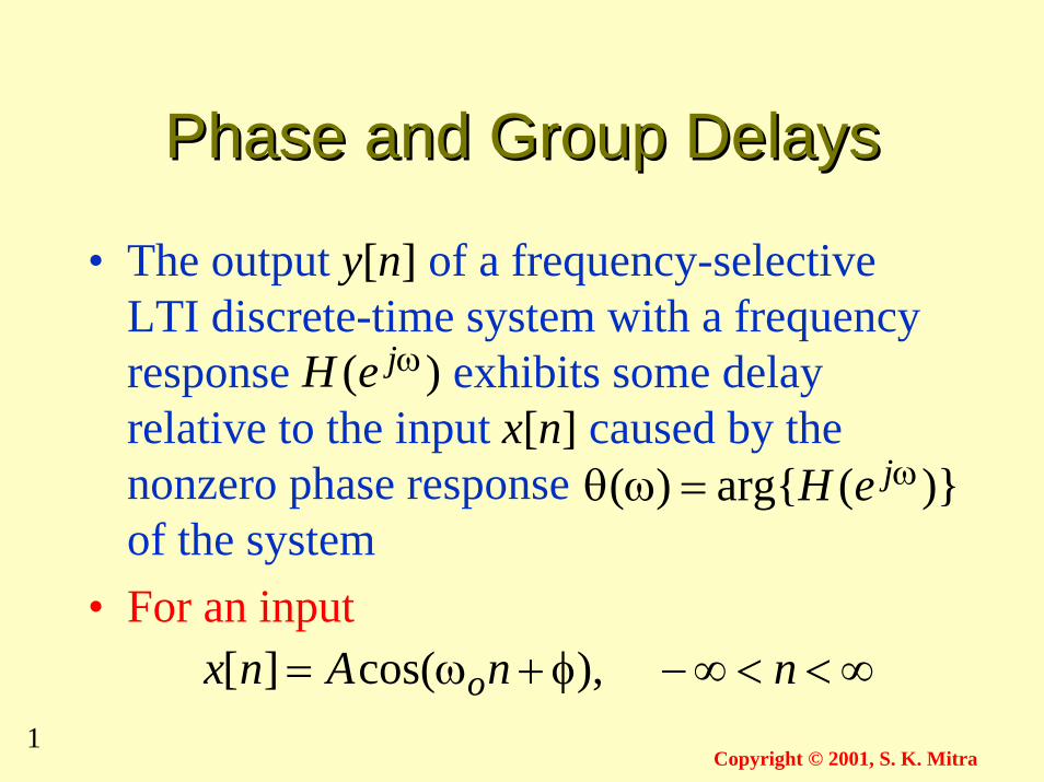
1 Copyright © 2001, S. K. Mitra Phase and Group Delays Phase and Group Delays • The output y[n] of a frequency-selective LTI discrete-time system with a frequency response exhibits some delay relative to the input x[n] caused by the nonzero phase response of the system • For an input ) ( ω j e H )} ( arg{ ) ( ω = ω θ j e H ∞ < < ∞ − φ + ω = n n A n x o ), cos( ] [
-
Upload
truongcong -
Category
Documents
-
view
214 -
download
0
Transcript of Phase and Group Delays - Signal and Image Processing...
1Copyright © 2001, S. K. Mitra
Phase and Group DelaysPhase and Group Delays
• The output y[n] of a frequency-selectiveLTI discrete-time system with a frequencyresponse exhibits some delayrelative to the input x[n] caused by thenonzero phase responseof the system
• For an input
)( ωjeH
)}(arg{)( ω=ωθ jeH
∞<<∞−φ+ω= nnAnx o ),cos(][
2Copyright © 2001, S. K. Mitra
Phase and Group DelaysPhase and Group Delays
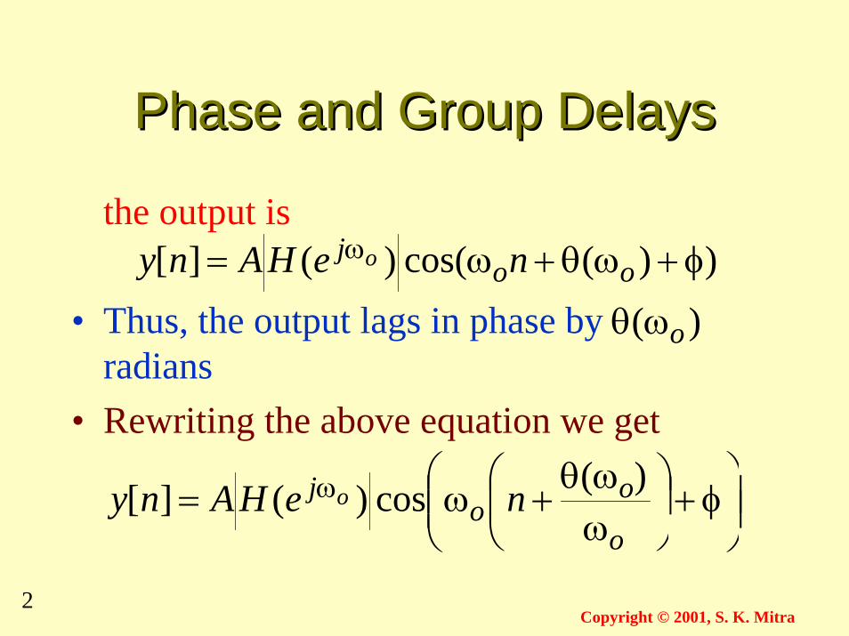
the output is
• Thus, the output lags in phase byradians
• Rewriting the above equation we get
))(cos()(][ φ+ωθ+ω= ωoo
j neHAny o
)( oωθ
φ+
ωωθ+ω= ω
o
oo
j neHAny o)(cos)(][
3Copyright © 2001, S. K. Mitra
Phase and Group DelaysPhase and Group Delays
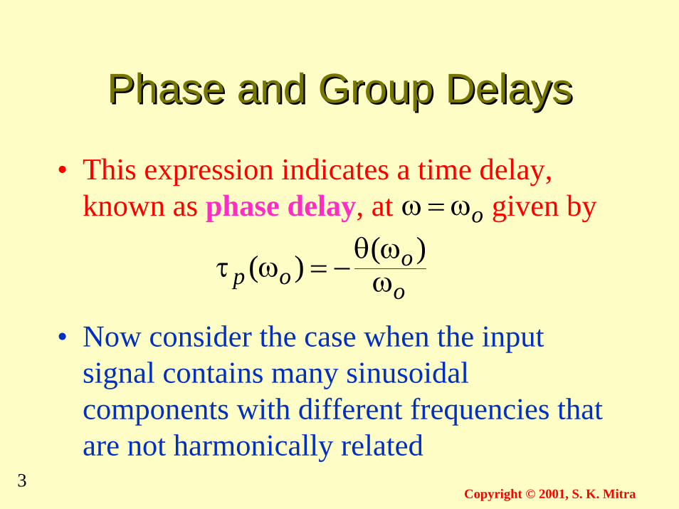
• This expression indicates a time delay,known as phase delay, at given by
• Now consider the case when the inputsignal contains many sinusoidalcomponents with different frequencies thatare not harmonically related
oω=ω
oo
op ωωθ
−=ωτ)()(
4Copyright © 2001, S. K. Mitra
Phase and Group DelaysPhase and Group Delays
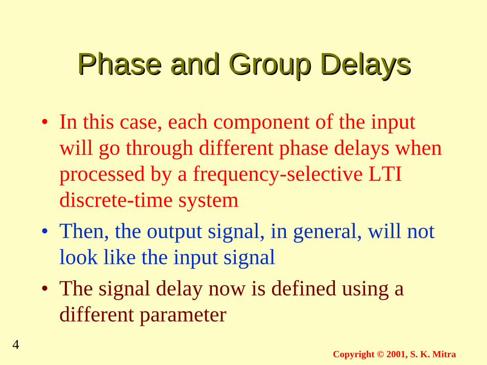
• In this case, each component of the inputwill go through different phase delays whenprocessed by a frequency-selective LTIdiscrete-time system
• Then, the output signal, in general, will notlook like the input signal
• The signal delay now is defined using adifferent parameter
5Copyright © 2001, S. K. Mitra
Phase and Group DelaysPhase and Group Delays
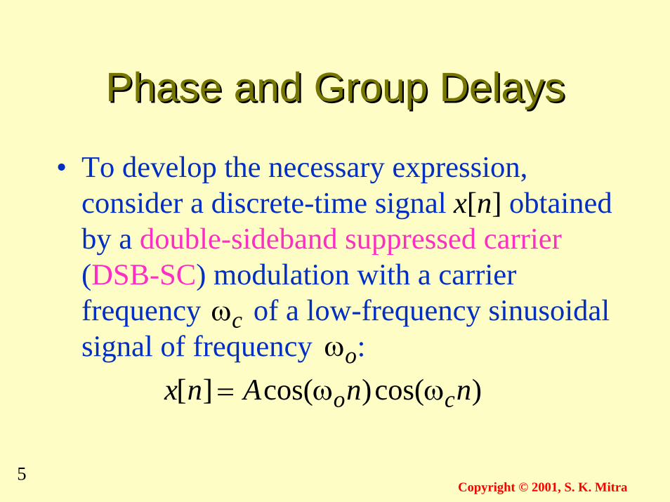
• To develop the necessary expression,consider a discrete-time signal x[n] obtainedby a double-sideband suppressed carrier(DSB-SC) modulation with a carrierfrequency of a low-frequency sinusoidalsignal of frequency :oω
cω
)cos()cos(][ nnAnx co ωω=
6Copyright © 2001, S. K. Mitra
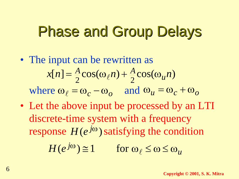
Phase and Group DelaysPhase and Group Delays
• The input can be rewritten as
where and• Let the above input be processed by an LTI
discrete-time system with a frequencyresponse satisfying the condition
)cos()cos(][22
nnnx uAA ω+ω= l
oc ω−ω=ωl ocu ω+ω=ω
)( ωjeH
ujeH ω≤ω≤ω≅ω
lfor1)(
7Copyright © 2001, S. K. Mitra
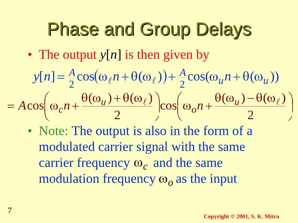
Phase and Group DelaysPhase and Group Delays• The output y[n] is then given by
• Note: The output is also in the form of amodulated carrier signal with the samecarrier frequency and the samemodulation frequency as the input
( ) ))(cos()(cos][22 uuAA nnny ωθ+ω+ωθ+ω= ll
ωθ−ωθ+ω
ωθ+ωθ+ω=
2)()(cos
2)()(cos ll u
ou
c nnA
cωoω
8Copyright © 2001, S. K. Mitra
Phase and Group DelaysPhase and Group Delays
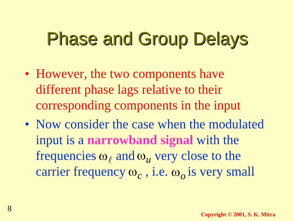
• However, the two components havedifferent phase lags relative to theircorresponding components in the input
• Now consider the case when the modulatedinput is a narrowband signal with thefrequencies and very close to thecarrier frequency , i.e. is very small
lω uωcω oω
9Copyright © 2001, S. K. Mitra
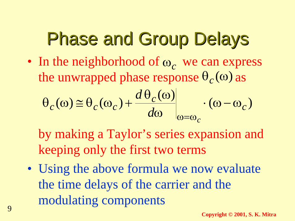
Phase and Group DelaysPhase and Group Delays• In the neighborhood of we can express
the unwrapped phase response as
by making a Taylor’s series expansion andkeeping only the first two terms
• Using the above formula we now evaluatethe time delays of the carrier and themodulating components
cω)(ωθc
)()()()( cc
cccc
dd ω−ω⋅
ωωθ+ωθ≅ωθ
ω=ω
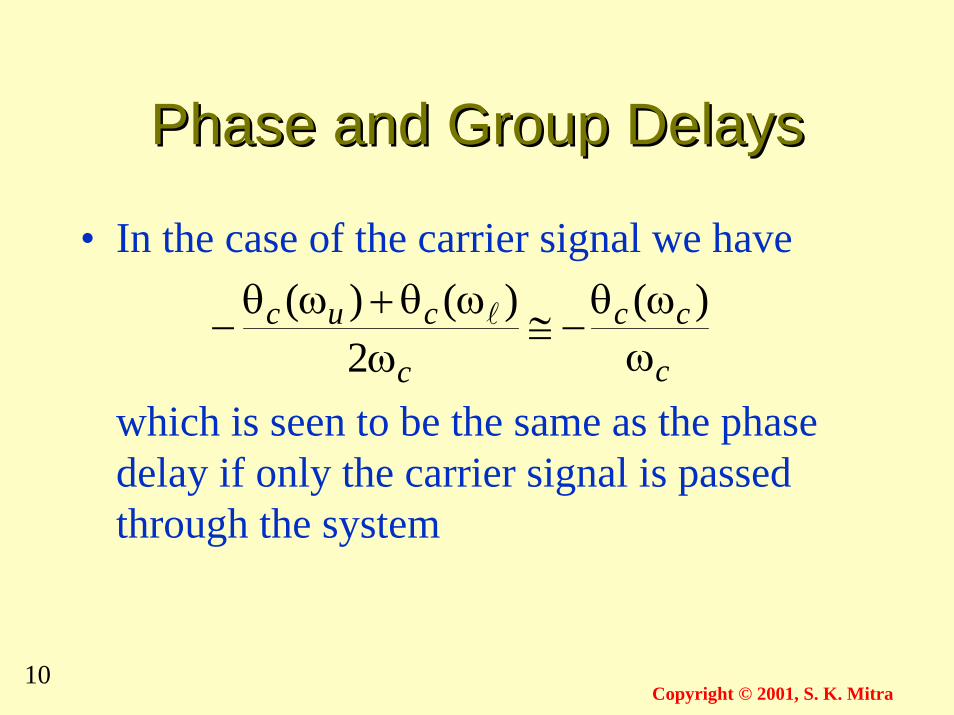
10Copyright © 2001, S. K. Mitra
Phase and Group DelaysPhase and Group Delays
• In the case of the carrier signal we have
which is seen to be the same as the phasedelay if only the carrier signal is passedthrough the system
c
cc
c
cucωωθ
−≅ω
ωθ+ωθ−
)(2
)()( l
11Copyright © 2001, S. K. Mitra
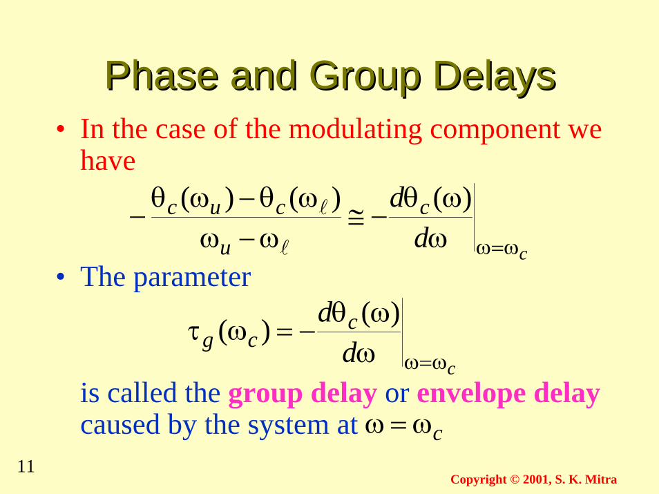
Phase and Group DelaysPhase and Group Delays• In the case of the modulating component we
have
• The parameter
is called the group delay or envelope delaycaused by the system at
cd
d c
u
cuc
ω=ωωωθ−≅
ω−ωωθ−ωθ− )()()(
l
l
cd
d ccg
ω=ωωωθ−=ωτ )()(
cω=ω
12Copyright © 2001, S. K. Mitra
Phase and Group DelaysPhase and Group Delays
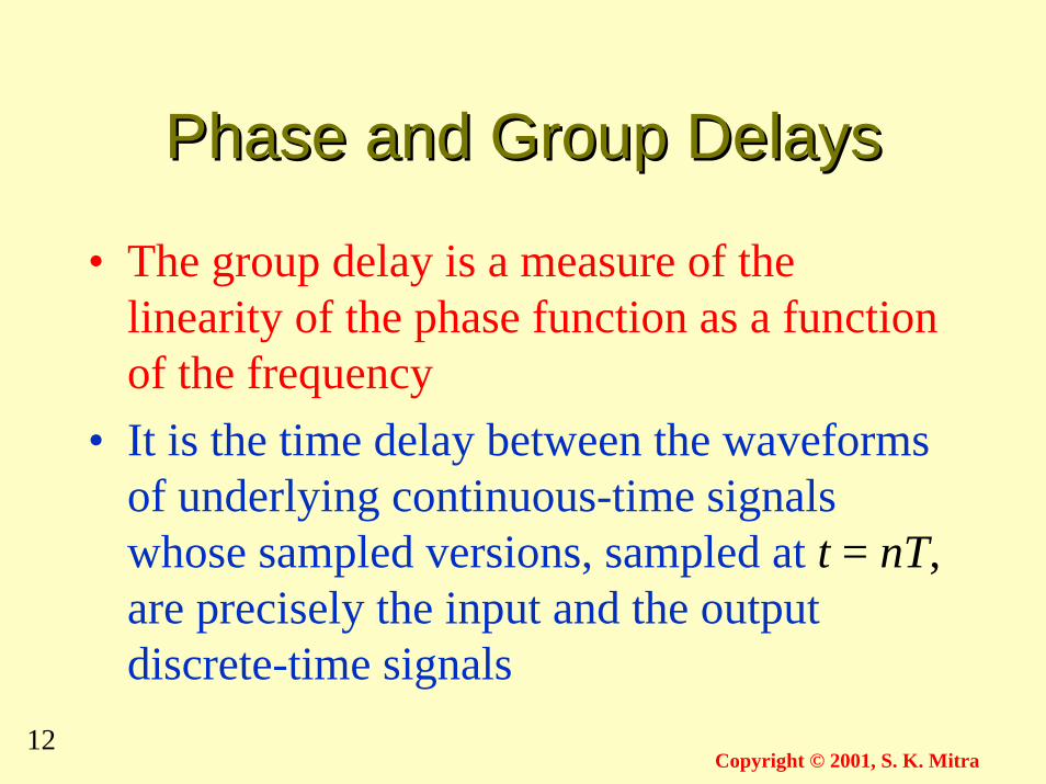
• The group delay is a measure of thelinearity of the phase function as a functionof the frequency
• It is the time delay between the waveformsof underlying continuous-time signalswhose sampled versions, sampled at t = nT,are precisely the input and the outputdiscrete-time signals
13Copyright © 2001, S. K. Mitra
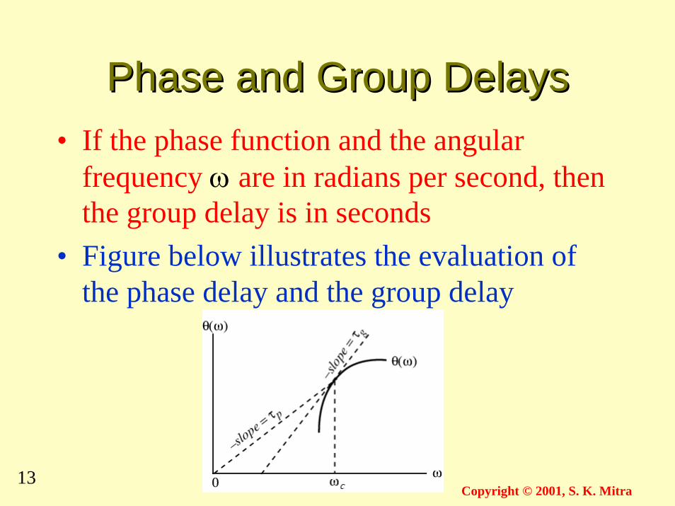
Phase and Group DelaysPhase and Group Delays• If the phase function and the angular
frequency ω are in radians per second, thenthe group delay is in seconds
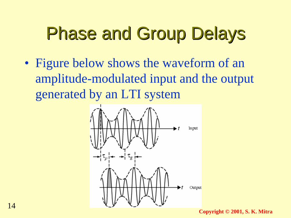
• Figure below illustrates the evaluation ofthe phase delay and the group delay
14Copyright © 2001, S. K. Mitra
Phase and Group DelaysPhase and Group Delays• Figure below shows the waveform of an
amplitude-modulated input and the outputgenerated by an LTI system
15Copyright © 2001, S. K. Mitra
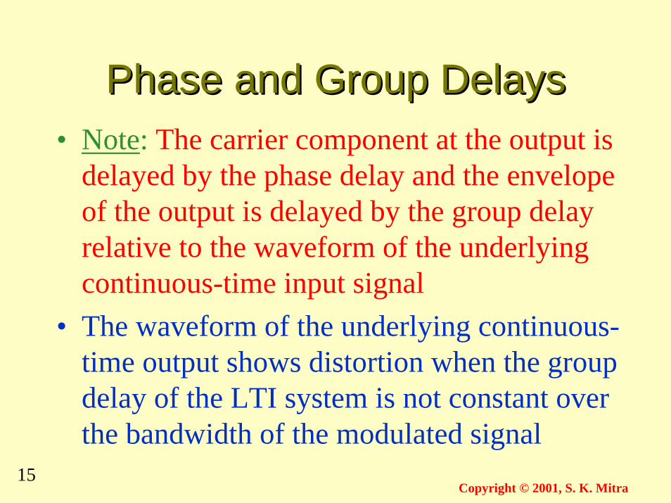
Phase and Group DelaysPhase and Group Delays• Note: The carrier component at the output is
delayed by the phase delay and the envelopeof the output is delayed by the group delayrelative to the waveform of the underlyingcontinuous-time input signal
• The waveform of the underlying continuous-time output shows distortion when the groupdelay of the LTI system is not constant overthe bandwidth of the modulated signal
16Copyright © 2001, S. K. Mitra
Phase and Group DelaysPhase and Group Delays
• If the distortion is unacceptable, a delayequalizer is usually cascaded with the LTIsystem so that the overall group delay of thecascade is approximately linear over the bandof interest
• To keep the magnitude response of the parentLTI system unchanged the equalizer musthave a constant magnitude response at allfrequencies
17Copyright © 2001, S. K. Mitra
Phase and Group DelaysPhase and Group Delays
• Example - The phase function of the FIRfilteris
• Hence its group delay is given byverifying the result obtained earlier bysimulation
][][][][ 21 −+−+= nxnxnxny αβαω−=ωθ )(
1)( =ωτg
18Copyright © 2001, S. K. Mitra
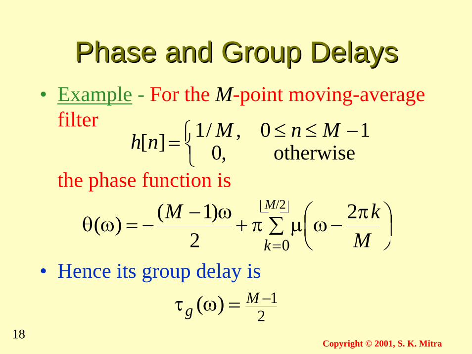
Phase and Group DelaysPhase and Group Delays• Example - For the M-point moving-average
filter
the phase function is
• Hence its group delay is
=][nh otherwise0
101,
,/ −≤≤ MnM
∑
π
−ωµπ+ω−
−=ωθ=0
22
)1()(k M
kM M/2
21)( −=ωτ M
g
19Copyright © 2001, S. K. Mitra
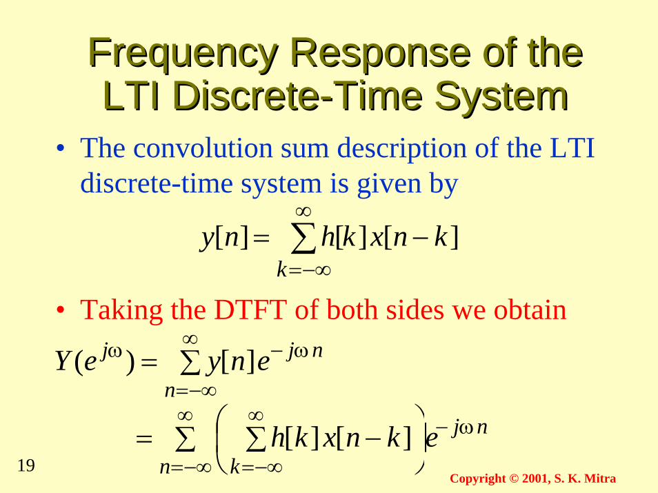
Frequency Response of theFrequency Response of theLTI Discrete-Time SystemLTI Discrete-Time System
• The convolution sum description of the LTIdiscrete-time system is given by
• Taking the DTFT of both sides we obtain
][][][ knxkhnyk
−= ∑∞
−∞=
nj
n
j enyeY ω−∞
−∞=
ω ∑= ][)(
nj
n keknxkh ω−∞
−∞=
∞
−∞=∑
∑ −= ][][
20Copyright © 2001, S. K. Mitra
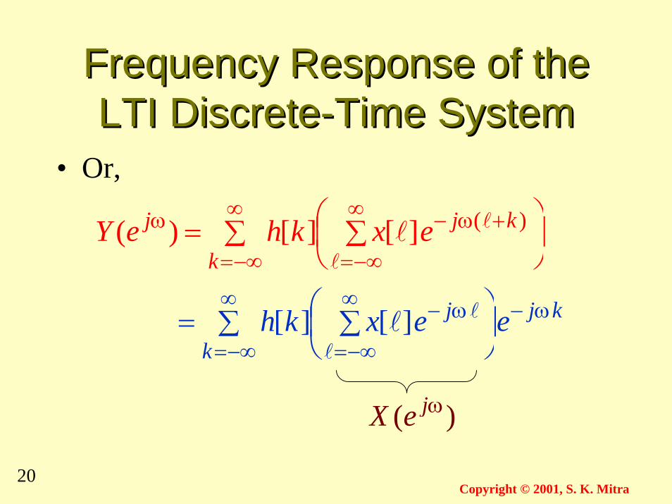
Frequency Response of theFrequency Response of theLTI Discrete-Time SystemLTI Discrete-Time System
• Or,
∑
∑=
∞
−∞=
∞
−∞=
+ω−ω
k
kjj exkheYl
ll )(][][)(
kj
k
j eexkh ω−∞
−∞=
∞
−∞=
ω−∑
∑=l
ll][][
)( ωjeX
21Copyright © 2001, S. K. Mitra
Frequency Response of theFrequency Response of theLTI Discrete-Time SystemLTI Discrete-Time System
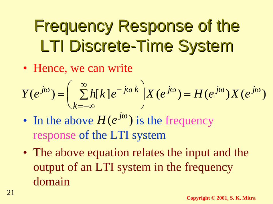
• Hence, we can write
• In the above is the frequencyresponse of the LTI system
• The above equation relates the input and theoutput of an LTI system in the frequencydomain
)()()(][)( ωωω∞
−∞=
ω−ω =
∑= jjj
k
kjj eXeHeXekheY
)( ωjeH
22Copyright © 2001, S. K. Mitra
Frequency Response of theFrequency Response of theLTI Discrete-Time SystemLTI Discrete-Time System
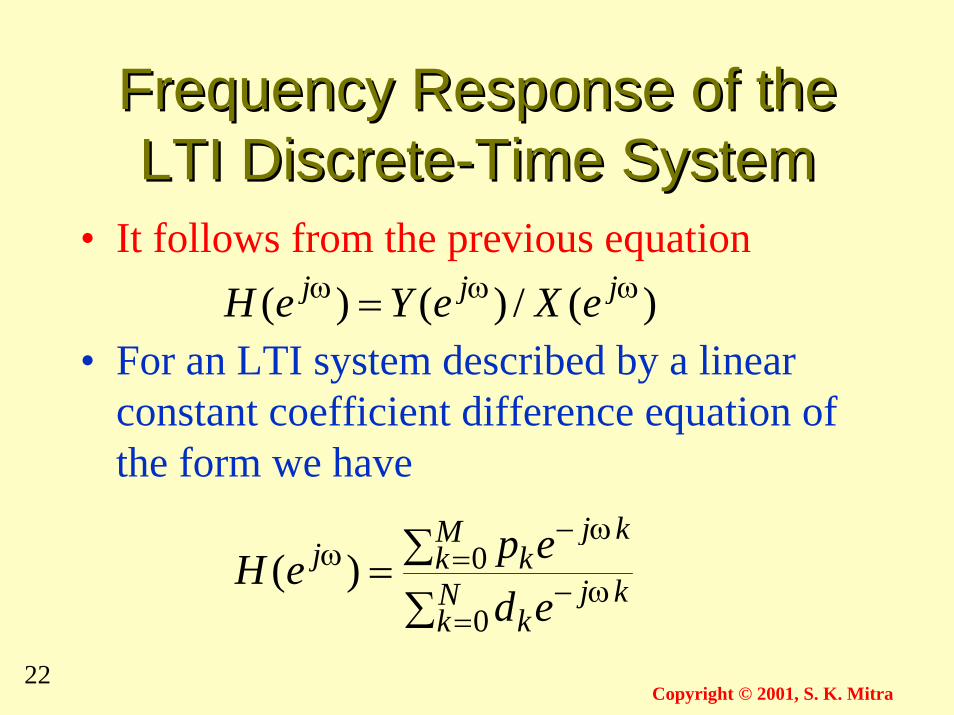
• It follows from the previous equation
• For an LTI system described by a linearconstant coefficient difference equation ofthe form we have
)(/)()( ωωω = jjj eXeYeH
∑∑=
=ω−
=ω−
ωNk
kjk
Mk
kjkj
edepeH
0
0)(
23Copyright © 2001, S. K. Mitra
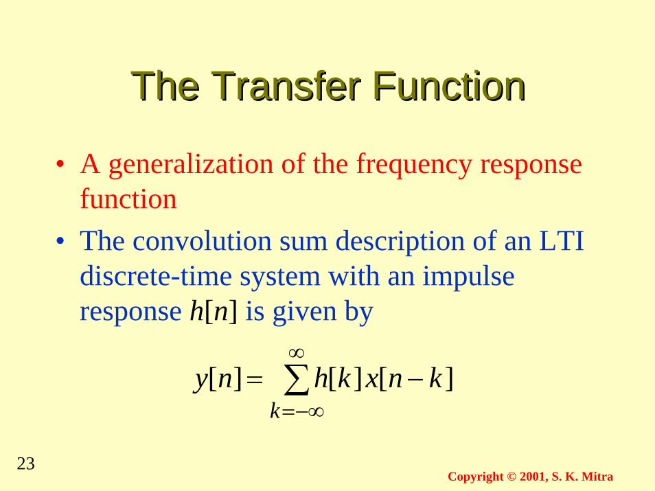
The Transfer FunctionThe Transfer Function
• A generalization of the frequency responsefunction
• The convolution sum description of an LTIdiscrete-time system with an impulseresponse h[n] is given by
∑∞
−∞=−=
kknxkhny ][][][
24Copyright © 2001, S. K. Mitra
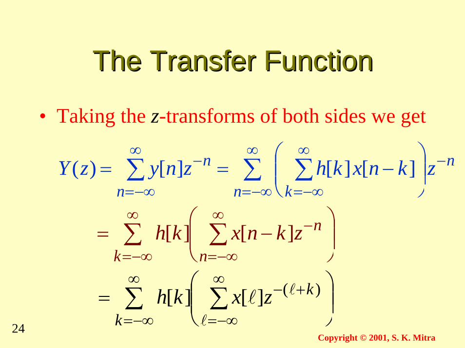
The Transfer FunctionThe Transfer Function
• Taking the z-transforms of both sides we get
n
n kn
n zknxkhznyzY −∞
−∞=
∞
−∞=
∞
−∞=
− ∑ ∑∑
−== ][][][)(
∑ ∑∞
−∞=
∞
−∞=
−
−=
k n
nzknxkh ][][
∑ ∑∞
−∞=
∞
−∞=
+−
=
k
kzxkhl
ll )(][][
25Copyright © 2001, S. K. Mitra
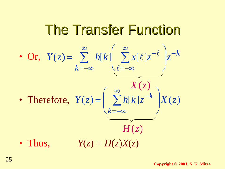
The Transfer FunctionThe Transfer Function
• Or,
• Therefore,
• Thus, Y(z) = H(z)X(z)
k
kzzxkhzY −
∞
−∞=
∞
−∞=
−∑ ∑
=
l
ll][][)(
)(zX)(][)( zXzkhzY
k
k
= ∑
∞
−∞=
−
)(zH
26Copyright © 2001, S. K. Mitra
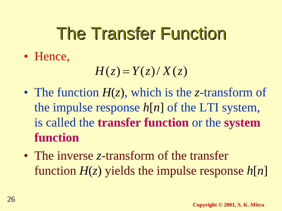
The Transfer FunctionThe Transfer Function• Hence,
• The function H(z), which is the z-transform ofthe impulse response h[n] of the LTI system,is called the transfer function or the systemfunction
• The inverse z-transform of the transferfunction H(z) yields the impulse response h[n]
)(/)()( zXzYzH =
27Copyright © 2001, S. K. Mitra
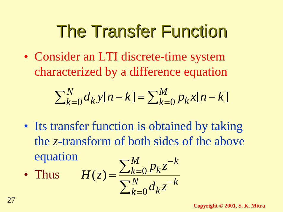
The Transfer FunctionThe Transfer Function• Consider an LTI discrete-time system
characterized by a difference equation
• Its transfer function is obtained by takingthe z-transform of both sides of the aboveequation
• Thus
∑∑ == −=− Mk k
Nk k knxpknyd 00 ][][
∑∑
=−
=−
= Nk
kk
Mk
kk
zd
zpzH
0
0)(
28Copyright © 2001, S. K. Mitra
The Transfer FunctionThe Transfer Function
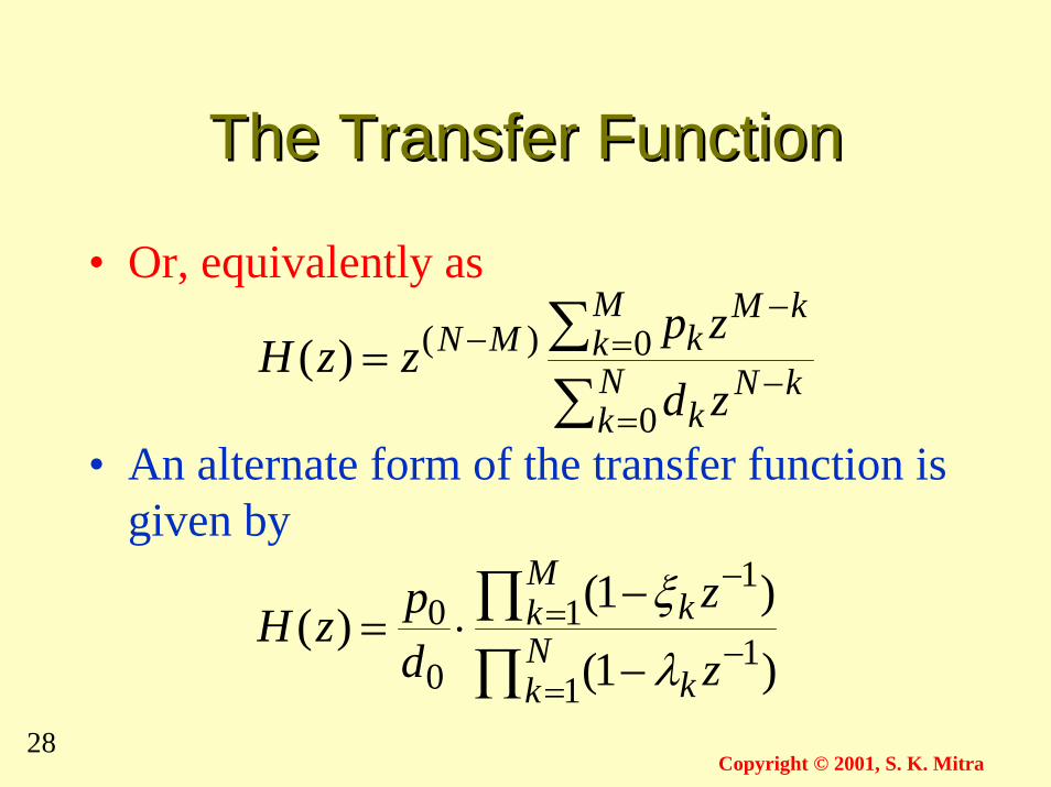
• Or, equivalently as
• An alternate form of the transfer function isgiven by
∑∑
=−
=−
−= Nk
kNk
Mk
kMkMN
zd
zpzzH
0
0)()(
∏∏
=−
=−
−
−⋅= N
k k
Mk k
z
zdpzH
11
11
0
0
1
1
)(
)()(
λ
ξ
29Copyright © 2001, S. K. Mitra
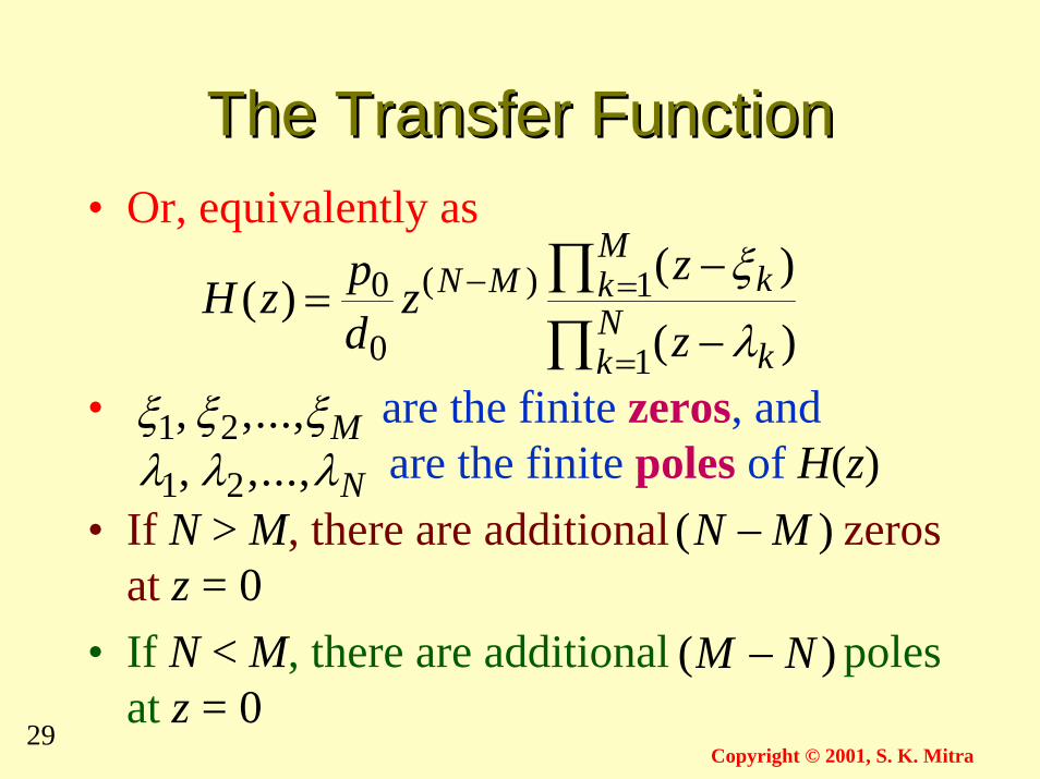
The Transfer FunctionThe Transfer Function• Or, equivalently as
• are the finite zeros, and are the finite poles of H(z)
• If N > M, there are additional zerosat z = 0
• If N < M, there are additional polesat z = 0
Mξξξ ,...,, 21Nλλλ ,...,, 21
)( MN −
)( NM −
∏∏
=
=−
−
−= N
k k
Mk kMN
z
zz
dpzH
1
1
0
0
)(
)()( )(
λ
ξ
30Copyright © 2001, S. K. Mitra
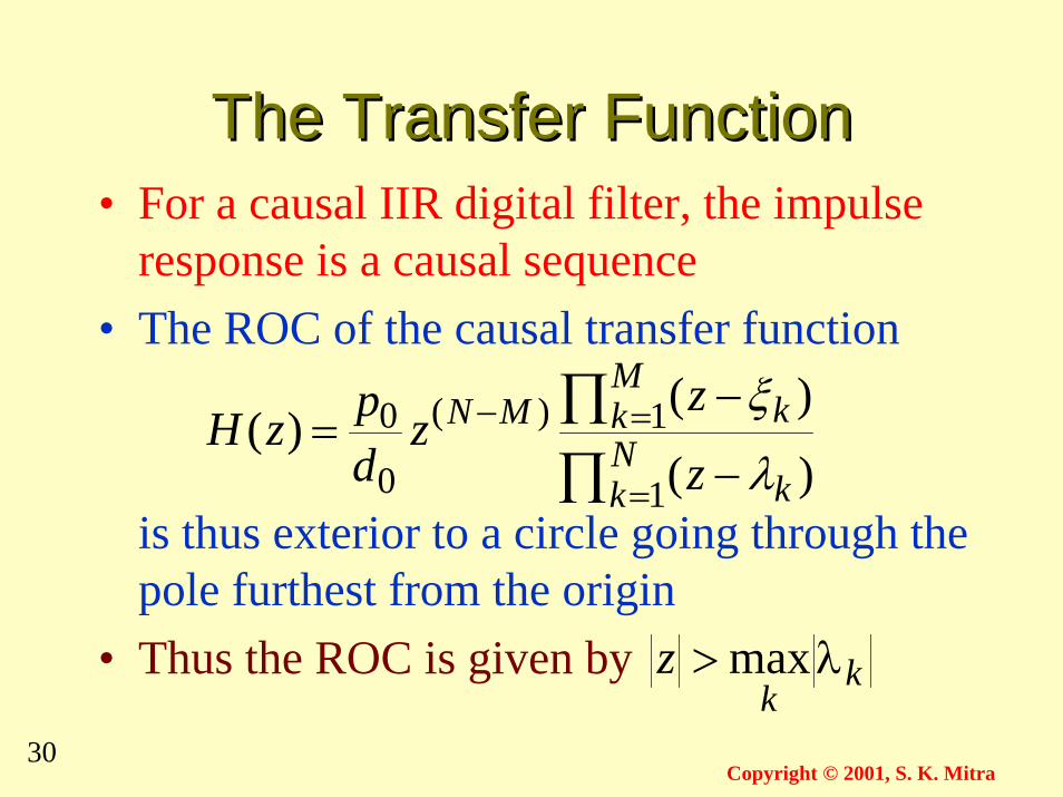
The Transfer FunctionThe Transfer Function• For a causal IIR digital filter, the impulse
response is a causal sequence• The ROC of the causal transfer function
is thus exterior to a circle going through thepole furthest from the origin
• Thus the ROC is given by
∏∏
=
=−
−
−= N
k k
Mk kMN
z
zz
dpzH
1
1
0
0
)(
)()( )(
λ
ξ
kk
z λ> max
31Copyright © 2001, S. K. Mitra
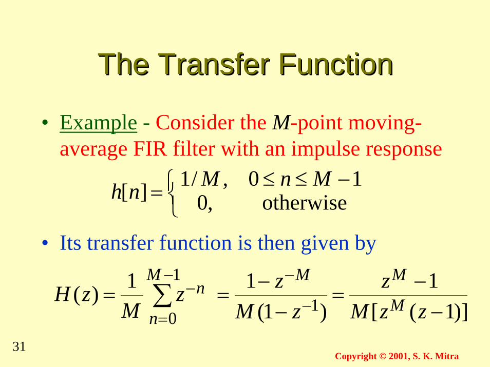
The Transfer FunctionThe Transfer Function
• Example - Consider the M-point moving-average FIR filter with an impulse response
• Its transfer function is then given by=][nh otherwise,0
10,/1 −≤≤ MnM
∑−
=
−=1
0
1)(M
n
nzM
zH)]1([
1)1(
11 −
−=−
−= −
−
zzMz
zMz
M
MM
32Copyright © 2001, S. K. Mitra
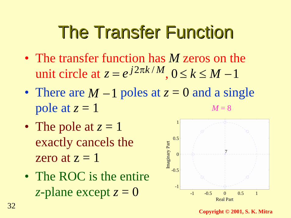
The Transfer FunctionThe Transfer Function• The transfer function has M zeros on the
unit circle at ,• There are poles at z = 0 and a single
pole at z = 1• The pole at z = 1
exactly cancels thezero at z = 1
• The ROC is the entirez-plane except z = 0
Mkjez /2π= 10 −≤≤ Mk
-1 -0.5 0 0.5 1
-1
-0.5
0
0.5
1
Real Part
Imag
inar
y P
art
7
M = 8
1−M
33Copyright © 2001, S. K. Mitra
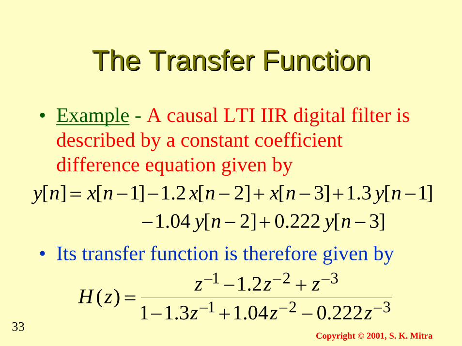
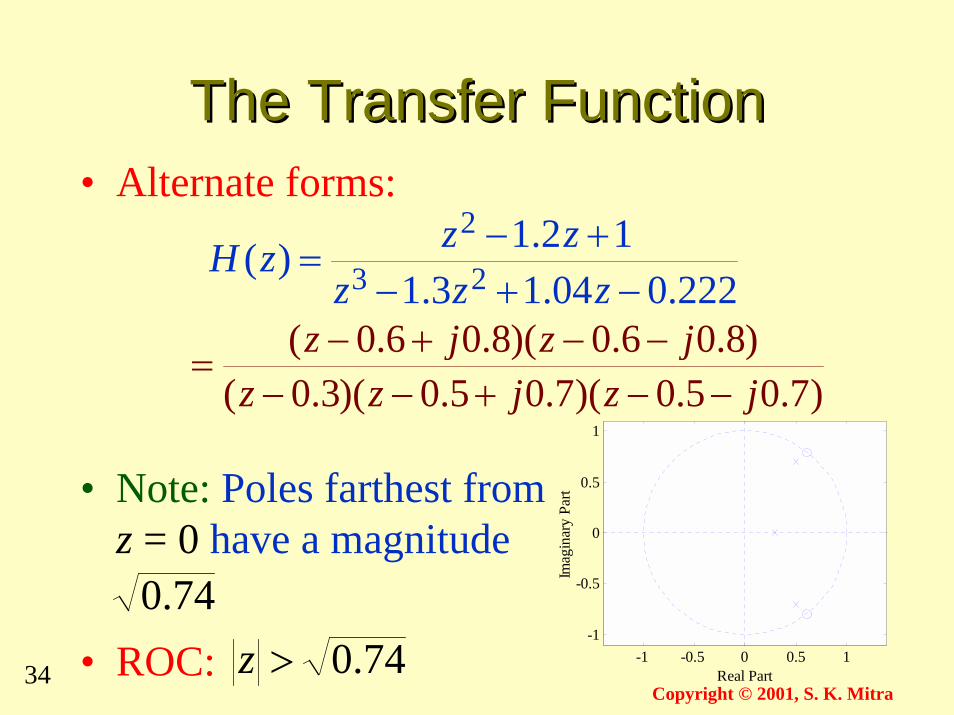
The Transfer FunctionThe Transfer Function
• Example - A causal LTI IIR digital filter isdescribed by a constant coefficientdifference equation given by
• Its transfer function is therefore given by
]1[3.1]3[]2[2.1]1[][ −+−+−−−= nynxnxnxny]3[222.0]2[04.1 −+−− nyny
321
321
222.004.13.112.1)( −−−
−−−
−+−+−=
zzzzzzzH
34Copyright © 2001, S. K. Mitra
The Transfer FunctionThe Transfer Function• Alternate forms:
• Note: Poles farthest fromz = 0 have a magnitude
• ROC:
222.004.13.112.1)( 23
2
−+−+−=zzz
zzzH
)7.05.0)(7.05.0)(3.0()8.06.0)(8.06.0(jzjzz
jzjz−−+−−
−−+−=
-1 -0.5 0 0.5 1
-1
-0.5
0
0.5
1
Real Part
Imag
inar
y P
art
74.0>z74.0
35Copyright © 2001, S. K. Mitra
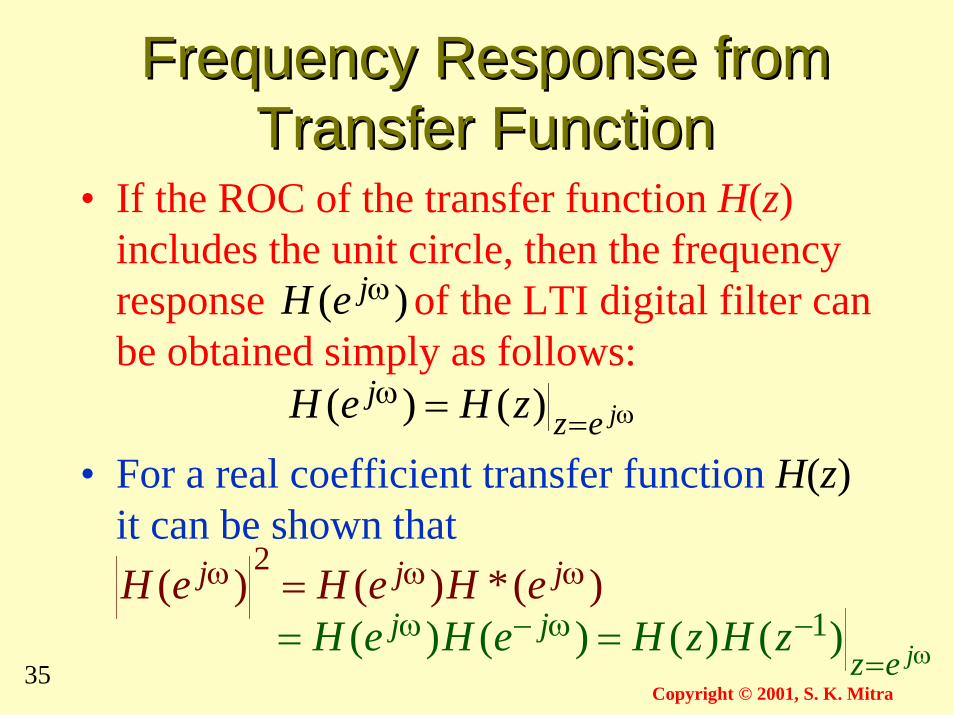
Frequency Response fromFrequency Response fromTransfer FunctionTransfer Function
• If the ROC of the transfer function H(z)includes the unit circle, then the frequencyresponse of the LTI digital filter canbe obtained simply as follows:
• For a real coefficient transfer function H(z)it can be shown that
ω=ω = jez
j zHeH )()(
)( ωjeH
)(*)()(2 ωωω = jjj eHeHeH
ω=−ω−ω == jez
jj zHzHeHeH )()()()( 1
36Copyright © 2001, S. K. Mitra
Frequency Response fromFrequency Response fromTransfer FunctionTransfer Function
• For a stable rational transfer function in theform
the factored form of the frequency responseis given by
∏∏
=
=−
−
−= N
k k
Mk kMN
z
zz
dpzH
1
1
0
0
)(
)()( )(
λ
ξ
∏∏
=ω
=ω
−ωω
λ−
ξ−= N
k kj
Mk k
jMNjj
e
ee
dpeH
1
1)(
0
0
)(
)()(
37Copyright © 2001, S. K. Mitra
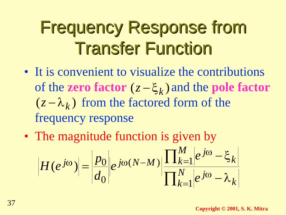
Frequency Response fromFrequency Response fromTransfer FunctionTransfer Function
• It is convenient to visualize the contributionsof the zero factor and the pole factor
from the factored form of thefrequency response
• The magnitude function is given by
)( kz ξ−)( kz λ−
∏∏
=ω
=ω
−ωω
λ−
ξ−= N
k kj
Mk k
jMNjj
e
ee
dpeH
1
1)(
0
0)(
38Copyright © 2001, S. K. Mitra
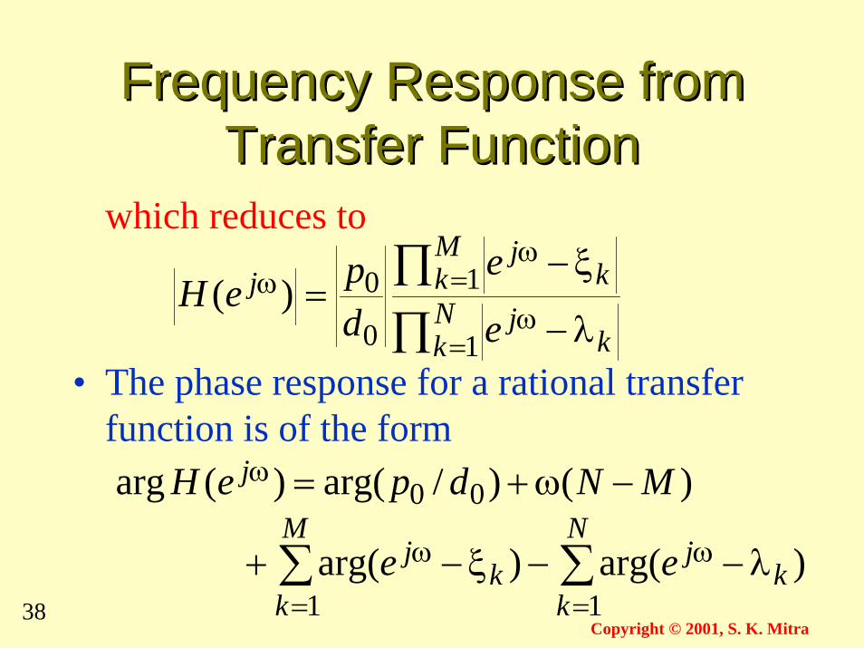
Frequency Response fromFrequency Response fromTransfer FunctionTransfer Function
which reduces to
• The phase response for a rational transferfunction is of the form
∏∏
=ω
=ω
ω
λ−
ξ−= N
k kj
Mk k
jj
e
edpeH
1
1
0
0)(
)()/arg()(arg 00 MNdpeH j −ω+=ω
∑∑=
ω
=
ω λ−−ξ−+N
kk
jM
kk
j ee11
)arg()arg(
39Copyright © 2001, S. K. Mitra
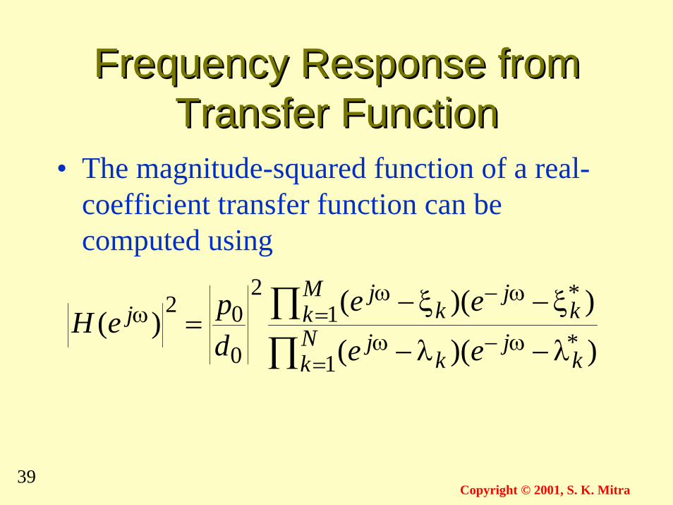
Frequency Response fromFrequency Response fromTransfer FunctionTransfer Function
• The magnitude-squared function of a real-coefficient transfer function can becomputed using
∏∏
=ω−ω
=ω−ω
ω
λ−λ−
ξ−ξ−= N
k kj
kj
Mk k
jk
jj
ee
eedpeH
1*
1*2
0
02
))((
))(()(
40Copyright © 2001, S. K. Mitra
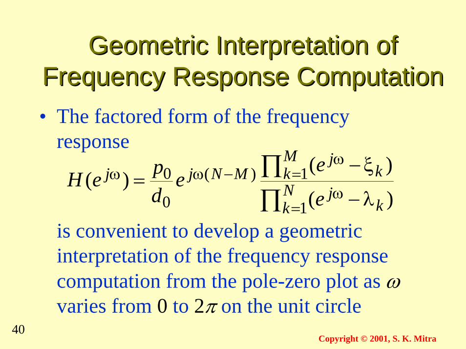
Geometric Interpretation ofGeometric Interpretation ofFrequency Response ComputationFrequency Response Computation• The factored form of the frequency
response
is convenient to develop a geometricinterpretation of the frequency responsecomputation from the pole-zero plot as ωvaries from 0 to 2π on the unit circle
∏∏
=ω
=ω
−ωω
λ−
ξ−= N
k kj
Mk k
jMNjj
e
ee
dpeH
1
1)(
0
0
)(
)()(
41Copyright © 2001, S. K. Mitra
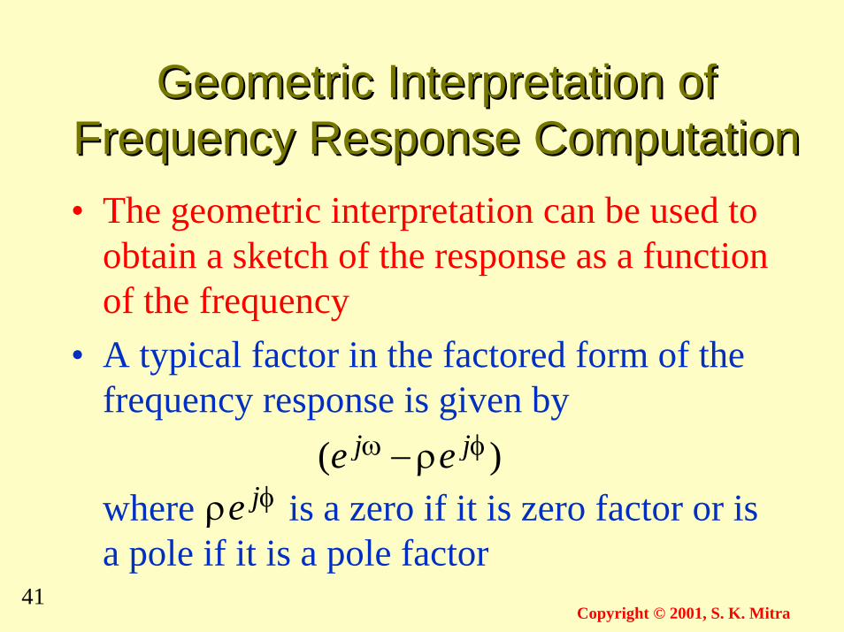
Geometric Interpretation ofGeometric Interpretation ofFrequency Response ComputationFrequency Response Computation• The geometric interpretation can be used to
obtain a sketch of the response as a functionof the frequency
• A typical factor in the factored form of thefrequency response is given by
where is a zero if it is zero factor or isa pole if it is a pole factor
)( φω ρ− jj eeφρ je
42Copyright © 2001, S. K. Mitra
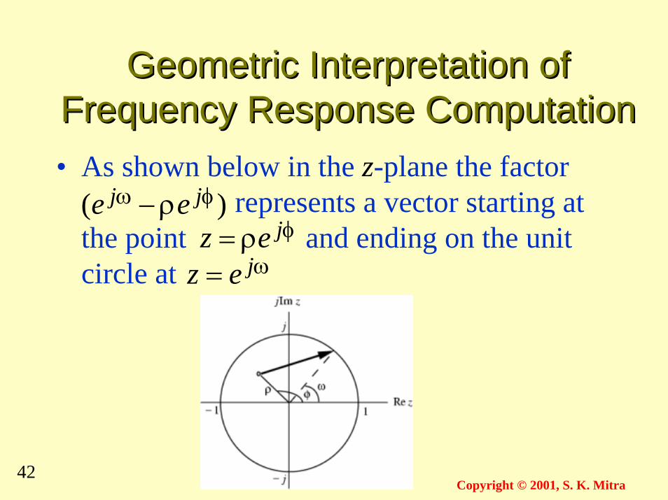
Geometric Interpretation ofGeometric Interpretation ofFrequency Response ComputationFrequency Response Computation• As shown below in the z-plane the factor
represents a vector starting atthe point and ending on the unitcircle at
φρ= jezω= jez
)( φω ρ− jj ee
43Copyright © 2001, S. K. Mitra
Geometric Interpretation ofGeometric Interpretation ofFrequency Response ComputationFrequency Response Computation
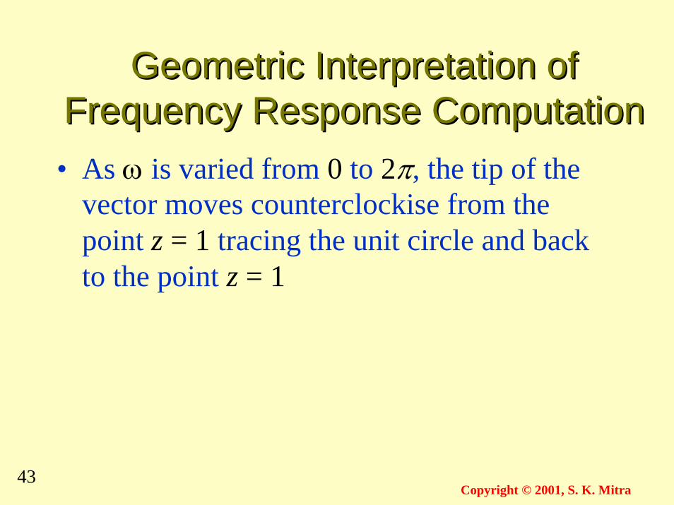
• As ω is varied from 0 to 2π, the tip of thevector moves counterclockise from thepoint z = 1 tracing the unit circle and backto the point z = 1
44Copyright © 2001, S. K. Mitra
Geometric Interpretation ofGeometric Interpretation ofFrequency Response ComputationFrequency Response Computation• As indicated by
the magnitude response at aspecific value of ω is given by the productof the magnitudes of all zero vectorsdivided by the product of the magnitudes ofall pole vectors
∏∏
=ω
=ω
ω
λ−
ξ−= N
k kj
Mk k
jj
e
edpeH
1
1
0
0)(
|)(| ωjeH
45Copyright © 2001, S. K. Mitra
Geometric Interpretation ofGeometric Interpretation ofFrequency Response ComputationFrequency Response Computation
• Likewise, from
we observe that the phase responseat a specific value of ω is obtained byadding the phase of the term and thelinear-phase term to the sum ofthe angles of the zero vectors minus theangles of the pole vectors
00 dp /)( MN −ω
)()/arg()(arg 00 MNdpeH j −ω+=ω
∑ λ−−∑ ξ−+ =ω
=ω N
k kjM
k kj ee 11 )arg()arg(
46Copyright © 2001, S. K. Mitra
Geometric Interpretation ofGeometric Interpretation ofFrequency Response ComputationFrequency Response Computation• Thus, an approximate plot of the magnitude
and phase responses of the transfer functionof an LTI digital filter can be developed byexamining the pole and zero locations
• Now, a zero (pole) vector has the smallestmagnitude when ω = φ
47Copyright © 2001, S. K. Mitra
Geometric Interpretation ofGeometric Interpretation ofFrequency Response ComputationFrequency Response Computation
• To highly attenuate signal components in aspecified frequency range, we need to placezeros very close to or on the unit circle inthis range
• Likewise, to highly emphasize signalcomponents in a specified frequency range,we need to place poles very close to or onthe unit circle in this range