Perceptron Homework - axon.cs.byu.edu

CS 478 - Perceptrons 1

Perceptron Homework

l  Assume a 3 input perceptron plus bias (it outputs 1 if net > 0, else 0) l  Assume a learning rate c of 1 and initial weights all 1: Δwi = c(t – z) xi l  Show weights after each pattern for just one epoch l  Training set 1 0 1 -> 0

1 1 0 -> 0 1 0 1 -> 1 0 1 1 -> 1

Pattern Target Weight Vector Net Output ΔW 1 0 1 1 0 1 1 1 1 3 1 -1 0 -1 -1 1 1 0 1 0 0 1 0 0 1 1 -1-1 0 -1 1 0 1 1 1 -1 0 0 -1 -2 0 1 0 1 1 0 1 1 1 1 0 0 1 0 1 1 0 0 0 0

0 0 1 0

Quadric Machine Homework l  Assume a 2 input perceptron expanded to be a quadric perceptron (it outputs 1 if

net > 0, else 0). Note that with binary inputs of -1, 1, that x2 and y2 would always be 1 and thus do not add info and are not needed (they would just act like to more bias weights)

l  Assume a learning rate c of .4 and initial weights all 0: Δwi = c(t – z) xi l  Show weights after each pattern for one epoch with the following non-linearly

separable training set. l  Has it learned to solve the problem after just one epoch? l  Which of the quadric features are actually needed to solve this training set?

CS 478 - Regression 2

x y Target

-1 -1 0

-1 1 1

1 -1 1

1 1 0

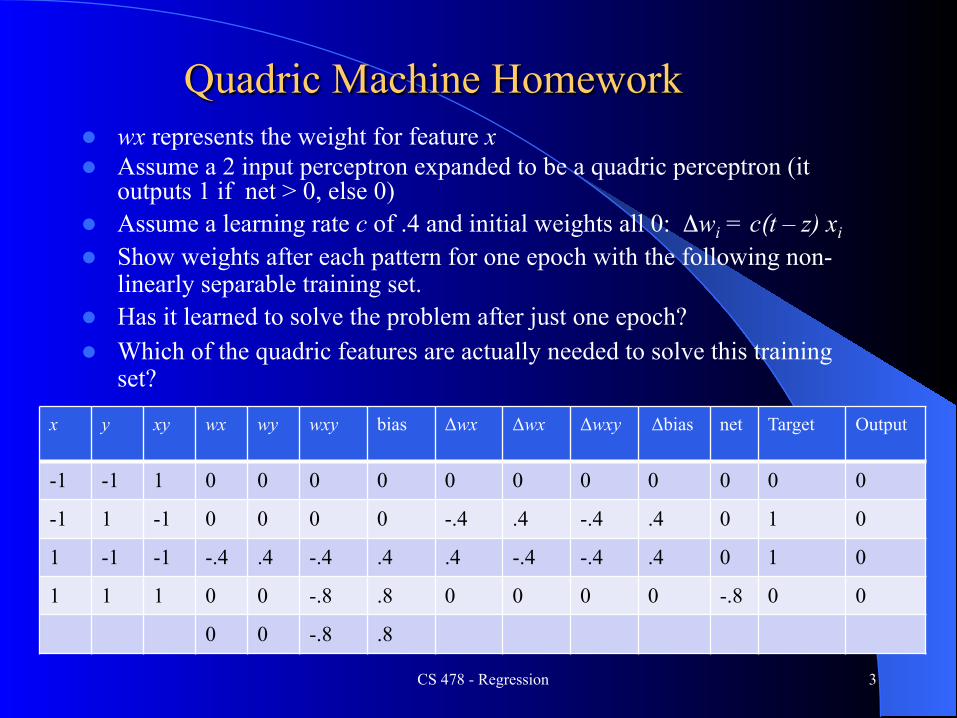
Quadric Machine Homework l  wx represents the weight for feature x l  Assume a 2 input perceptron expanded to be a quadric perceptron (it

outputs 1 if net > 0, else 0) l  Assume a learning rate c of .4 and initial weights all 0: Δwi = c(t – z) xi l  Show weights after each pattern for one epoch with the following non-

linearly separable training set. l  Has it learned to solve the problem after just one epoch? l  Which of the quadric features are actually needed to solve this training

set?


x y xy wx wy wxy bias Δwx Δwx

Δwxy

Δbias net Target Output

-1 -1 1 0 0 0 0 0 0 0 0 0 0 0

-1 1 -1 0 0 0 0 -.4 .4 -.4 .4 0 1 0

1 -1 -1 -.4 .4 -.4 .4 .4 -.4 -.4 .4 0 1 0

1 1 1 0 0 -.8 .8 0 0 0 0 -.8 0 0

0 0 -.8 .8

Quadric Machine Homework l  wx represents the weight for feature x l  Assume a 2 input perceptron expanded to be a quadric perceptron (it

outputs 1 if net > 0, else 0) l  Assume a learning rate c of .4 and initial weights all 0: Δwi = c(t – z) xi l  Show weights after each pattern for one epoch with the following non-

linearly separable training set. l  Has it learned to solve the problem after just one epoch? - Yes l  Which of the quadric features are actually needed to solve this training

set? – Really only needs feature xy.


x y xy wx wy wxy bias Δwx Δwx

Δwxy

Δbias net Target Output

-1 -1 1 0 0 0 0 0 0 0 0 0 0 0

-1 1 -1 0 0 0 0 -.4 .4 -.4 .4 0 1 0

1 -1 -1 -.4 .4 -.4 .4 .4 -.4 -.4 .4 0 1 0

1 1 1 0 0 -.8 .8 0 0 0 0 -.8 0 0

0 0 -.8 .8

Linear Regression Homework

l  Assume we start with all weights as 0 (don’t forget the bias)

l  What are the new weights after one iteration through the following training set using the delta rule with a learning rate of .2

CS 478 - Homework 5

x y Target

.3 .8 .7

-.3 1.6 -.1

.9 0 1.3

Linear Regression Homework

l  Assume we start with all weights as 0 (don’t forget the bias) l  What are the new weights after one iteration through the

following training set using the delta rule with a learning rate c = .2

CS 478 - Homework 6

x y Target

Net

w1 w2 Bias

0 0 0

.3 .8 .7 0 .042 .112 .140

-.3 1.6 -.1 .307 .066 -.018 .059

.9 0 1.3 .118 .279 -.018 .295

0 + .2(.7 – 0).3 = .042

Δwi = c(t − net)xi

Logistic Regression Homework

l  You don’t actually have to come up with the weights for this one, though you could quickly by using the closed form linear regression approach

l  Sketch each step you would need to learn the weights for the following data set using logistic regression

l  Sketch how you would generalize the probability of a heart attack given a new input heart rate of 60

CS 478 - Homework 7

Heart Rate Heart Attack

50 Y

50 N

50 N

50 N

70 N

70 Y

90 Y

90 Y

90 N

90 Y

90 Y

Logistic Regression Homework

1.  Calculate probabilities or odds for each input value 2.  Calculate the log odds 3.  Do linear regression on these 3 points to get the logit line 4.  To find the probability of a heart attack given a new input heart

rate of 60, just calculate p = elogit(60)/(1+elogit(60)) where logit(60) is the value on the logit line for 60

CS 478 - Homework 8

Heart Rate Heart Attack

50 Y

50 N

50 N

50 N

70 N

70 Y

90 Y

90 Y

90 N

90 Y

90 Y

Heart Rate Heart Attacks

Total Patients

Probability: # attacks/Total Patients

Odds: p/(1-p) = # attacks/ # not

Log Odds: ln(Odds)

50 1 4 .25 .33 -1.11 70 1 2 .5 1 0 90 4 5 .8 4 1.39

CS 478 – Backpropagation 9

BP-1) A 2-2-1 backpropagation model has initial weights as shown. Work through one cycle of learning for the f ollowing pattern(s). Assume 0 momentum and a learning constant of 1. Round calculations to 3 significant digits to the right of the decimal. Give values for all nodes and links for activation, output, error signal, weight delta, and final weights. Nodes 4, 5 , 6, and 7 are just input nodes and do not have a sigmoidal output. For each node calculate the following (show necessary equati on for each). Hint: Calculate bottom-top-bottom. a = o =

= w =

w =

1

2 3

7

+1

4

+1

65

a) All weights initially 1.0 Training Patterns 1) 0 0 -> 1 2) 0 1 -> 0


BP-1) net2 = wi xi = (1*0 + 1*0 + 1*1) = 1 net3 = 1 o2 = 1/(1+e-net) = 1/(1+e-1) = 1/(1+.368) = .731 o3 = .731 o4 = 1 net1 = (1*.731 + 1*.731 + 1) = 2.462 o1 = 1/(1+e-2.462)= .921

1 = (t1 - o1) o1 (1 - o1) = (1 - .921) .921 (1 - .921) = .00575 w21 = j oi = 1 o2 = 1 * .00575 * .731 = .00420 w31 = 1 * .00575 * .731 = .00420 w41 = 1 * .00575 * 1 = .00575 2 = oj (1 - oj) k wjk = o2 (1 - o2) 1 w21 =

. 7 3 1 ( 1 - .731) (.00575 * 1) = .00113 3 = .00113 w52 = j oi = 2 o5 = 1 * .00113 * 0 = 0 w62 = 0 w72 = 1 * .00113 * 1 = .00113 w53 = 0 w63 = 0 w73 = 1 * .00113 * 1 = .00113

1

2 3

7

+1

4

+1

65


Second pass for 0 1 -> 0 Modified Weights: w21 = 1.0042 w31 = 1.0042 w41 = 1.00575 w52 = 1 w62 = 1 w72 = 1.00113 w53 = 1 w63 = 1 w73 = 1.00113 net2 = wi xi = (1*0 + 1*1 + 1*1.00113) = 2.00113 net3 = 2.00113 o2 = 1/(1+e-net) = 1/(1+e-2.00113) = .881 o3 = .881 o4 = 1 net1 = (1.0042*.881 + 1.0042*.881 + 1.00575*1) = 2.775 o1 = 1/(1+e-2.775)= .941 1 = (t1 - o1) o1 (1 - o1) = (0 - .941) .941 (1 - .941) = -.0522 w21 = j oi = 1 o2 = 1 * -.0522 * .881 = -.0460 w31 = 1 * -.0522 * .881 = -.0460 w41 = 1 * -.0522 * 1 = -.0522 2 = oj (1 - oj) k wjk = o2 (1 - o2) 1 w21 =

. 8 8 1 ( 1 - .881) (-.0522 * 1.0042) = -.00547 3 = -.00547 w52 = j oi = 2 o5 = 1 * -.00547* 0 = 0 w62 = 1 * (-.00547) * 1 = -.00547 w72 = 1 * (-.00547) * 1 = -.00547 w53 = 0 w63 = -.00547 w73 = 1 * (-.00547) * 1 = -.00547

w21 = 1.0042 - .0460 = .958 w31 = 1.0042 - .0460 = .958 w41 = 1.00575 - .0522 = .954 w52 = 1 + 0 = 1 w62 = 1 - .00547 = .995 w72 = 1.00113 - .00547 = .996 w53 = 1 + 0 = 1 w63 = 1 - .00547 = .995 w73 = 1.00113 - .00547 = .996

PCA Homework

CS 478 - Homework 12

Original Data

x y

p1 .2 -.3

p2 -1.1 2

p3 1 -2.2

p4 .5 -1

p5 -.6 1

mean 0 -.1

Terms

m 5 Number of instances in data set

n 2 Number of input features

p 1 Final number of principal components chosen

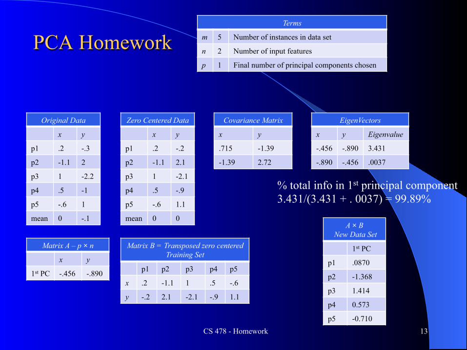
•  Use PCA on the given data set to get a transformed data set with just one feature (the first principal component (PC)). Show your work along the way.

•  Show what % of the total information is contained in the 1st PC.

•  Do not use a PCA package to do it. You need to go through the steps yourself, or program it yourself.

•  You may use a spreadsheet, Matlab, etc. to do the arithmetic for you.

•  You may use any web tool or Matlab to calculate the eigenvectors from the covariance matrix.

PCA Homework


Original Data

x y

p1 .2 -.3

p2 -1.1 2

p3 1 -2.2

p4 .5 -1

p5 -.6 1

mean 0 -.1

Zero Centered Data

x y

p1 .2 -.2

p2 -1.1 2.1

p3 1 -2.1

p4 .5 -.9

p5 -.6 1.1

mean 0 0

Covariance Matrix

x y

.715 -1.39

-1.39 2.72

EigenVectors

x y Eigenvalue

-.456 -.890 3.431

-.890 -.456 .0037

% total info in 1st principal component 3.431/(3.431 + . 0037) = 99.89%

Matrix A – p × n

x y

1st PC -.456 -.890

Terms

m 5 Number of instances in data set

n 2 Number of input features

p 1 Final number of principal components chosen

Matrix B = Transposed zero centered Training Set

p1 p2 p3 p4 p5

x .2 -1.1 1 .5 -.6

y -.2 2.1 -2.1 -.9 1.1

A × B New Data Set

1st PC

p1 .0870

p2 -1.368

p3 1.414

p4 0.573

p5 -0.710

Decision Tree Homework

l  Info(S) = - 2/9·log22/9 - 4/9·log24/9 -3/9·log23/9 = 1.53 –  Not necessary unless you want to calculate information gain

l  Starting with all instances, calculate gain for each attribute l  Let’s do Meat: l  InfoMeat(S) = 4/9·(-2/4log22/4 - 2/4·log22/4 - 0·log20/4) + 5/9·(-0/5·log20/5 - 2/5·log22/5 - 3/5·log23/5) = .98

–  Information Gain is 1.53 - .98 = .55 l  Finish this level, find best attribute and split, and then find the

best attribute for at least the left most node at the next level –  Assume sub-nodes are sorted alphabetically left to right by attribute

CS 478 - Decision Trees 14

Meat N,Y

Crust D,S,T

Veg N,Y

Quality B,G,Gr

Y Thin N Great

N Deep N Bad

N Stuffed Y Good

Y Stuffed Y Great

Y Deep N Good

Y Deep Y Great

N Thin Y Good

Y Deep N Good

N Thin N Bad

Info(S) = − pii=1

|C|

∑ log2(pi )

InfoA (S) =| Sj || S |

Info(Sj )i= j

|A|

∑ = −| Sj || S |

⋅ pii=1

|C|

∑ log2(pi )j=1

|A|

∑


l  InfoMeat(S) = 4/9·(-2/4log22/4 - 2/4·log22/4 - 0·log20/4) + 5/9·(-0/5·log20/5 - 2/5·log22/5 - 3/5·log23/5) = .98 l  InfoCrust(S) = 4/9·(-1/4log21/4 - 2/4·log22/4 - 1/4·log21/4) + 2/9·(-0/2·log20/2 - 1/2·log21/2 - 1/2·log21/2) + 3/9·(-1/3·log21/3 - 1/3·log21/3 - 1/3·log21/3) = 1.41 l  InfoVeg(S) = 5/9·(-2/5log22/5 - 2/5·log22/5 - 1/5·log21/5) + 4/9·(-0/4·log20/4 - 2/4·log22/4 - 2/4·log22/4) = 1.29 l  Attribute with least remaining info is Meat


MeatN,Y

Crust D,S,T

VegN,Y

Quality B,G,Gr

Y Thin N Great

N Deep N Bad

N Stuffed Y Good

Y Stuffed Y Great

Y Deep N Good

Y Deep Y Great

N Thin Y Good

Y Deep N Good

N Thin N Bad

Info(S) = − pii=1

|C|

∑ log2(pi )


Info(Sj )i= j

|A|

∑ = −| Sj || S |

⋅ pii=1

|C|

∑ log2(pi )j=1

|A|

∑


l  Left most node will be Meat = N containing 4 instances l  InfoCrust(S) = 1/4·(-1/1log21/1 - 0/1·log20/1 - 0/1·log20/1) + 1/4·(-0/1·log20/1 - 1/1·log21/1 - 0/1·log20/1) + 2/4·(-1/2·log21/2 - 1/2·log21/2 - 0/2·log20/2) = .5 l  InfoVeg(S) = 2/4·(-2/2log22/2 - 0/2·log20/2 - 0/2·log20/2) + 2/4·(-0/2·log20/2 - 2/2·log22/2 - 0/2·log20/2) = 0 l  Attribute with least remaining info is Veg which will split

into two pure nodes


MeatN,Y

Crust D,S,T

VegN,Y

Quality B,G,Gr

N Deep N Bad

N Stuffed Y Good

N Thin Y Good

N Thin N Bad Info(S) = − pii=1

|C|

∑ log2(pi )


Info(Sj )i= j

|A|

∑ = −| Sj || S |

⋅ pii=1

|C|

∑ log2(pi )j=1

|A|

∑

k-Nearest Neighbor Homework

l  Assume the following training set. l  Assume a new point (.5, .2)

–  For nearest neighbor distance use Manhattan distance –  What would the output be for 3-nn with no distance weighting?

Show work and vote. –  What would the output be for 3-nn with distance weighting? Show

work and vote.


x y Target

.3 .8 A

-.3 1.6 B

.9 0 B

1 1 A

k-Nearest Neighbor Homework

l  Assume the following training set. l  Assume a new point (.5, .2)

–  For nearest neighbor distance use Manhattan distance –  What would the output be for 3-nn with no distance weighting?– A

wins with vote 2/3 –  What would the output be for 3-nn with distance weighting? A has

vote 1/.82 + 1/1.32 = 2.15, B wins with vote 1/.42 = 6.25


x y distance Target

.3 .8 .2 + .6 = .8 A

-.3 1.6 .8 + 1.4 = 2.2 B

.9 .0 .4 + .2 = .6 B

1 1 .5 + .8 = 1.3 A

RBF Homework l  Assume you have an RBF with

–  Two inputs –  Three output classes A, B, and C (linear units) –  Three prototype nodes at (0,0), (.5,1) and (1,.5) –  The radial basis function of the prototype nodes is

l  max(0, 1 – Manhattan distance between the prototype node and the instance)

–  Assume no bias and initial weights of .6 into output node A, -.4 into output node B, and 0 into output node C

–  Assume top layer training is the delta rule with LR = .1

l  Assume we input the single instance .6 .8 –  Which class would be the winner? –  What would the weights be updated to if it were a training instance

of .6 .8 with target class B?


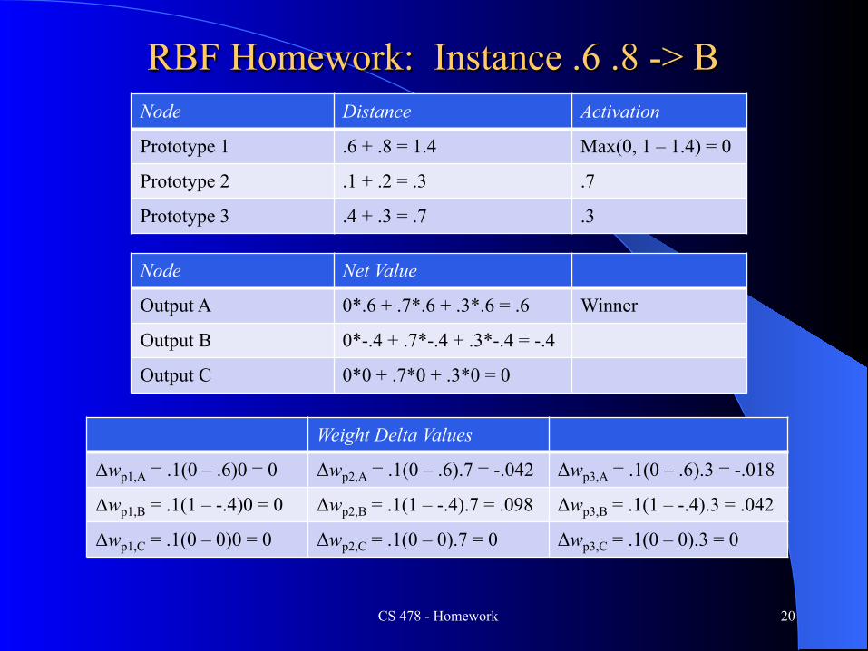
RBF Homework: Instance .6 .8 -> B


Node Distance Activation

Prototype 1 .6 + .8 = 1.4 Max(0, 1 – 1.4) = 0

Prototype 2 .1 + .2 = .3 .7

Prototype 3 .4 + .3 = .7 .3

Node Net Value

Output A 0*.6 + .7*.6 + .3*.6 = .6 Winner

Output B 0*-.4 + .7*-.4 + .3*-.4 = -.4

Output C 0*0 + .7*0 + .3*0 = 0

Weight Delta Values

Δwp1,A = .1(0 – .6)0 = 0 Δwp2,A = .1(0 – .6).7 = -.042 Δwp3,A = .1(0 – .6).3 = -.018

Δwp1,B = .1(1 – -.4)0 = 0 Δwp2,B = .1(1 – -.4).7 = .098 Δwp3,B = .1(1 – -.4).3 = .042

Δwp1,C = .1(0 – 0)0 = 0 Δwp2,C = .1(0 – 0).7 = 0 Δwp3,C = .1(0 – 0).3 = 0

Size (B, S)

Color (R,G,B)

Output (P,N)

B R P

S B P

S B N

B R N

B B P

B G N

S B P

CS 478 - Bayesian Learning 21 €

vNB = argmaxv j ∈V

P(v j ) P(ai | v j )i∏

For the given training set: 1.  Create a table of the statistics

needed to do Naïve Bayes 2.  What would be the output for a

new instance which is Small and Blue?

3.  What is the Naïve Bayes value and the normalized probability for each output class (P or N) for this case of Small and Blue?

Naïve Bayes Homework

HAC Homework

l  For the data set below show all iterations (from 5 clusters until 1 cluster remaining) for HAC single link. Show work. Use Manhattan distance. In case of ties go with the cluster containing the least alphabetical instance. Show the dendrogram for the HAC case, including properly labeled distances on the vertical-axis of the dendrogram.

CS 478 - Clustering 23

Pattern x y

a .8 .7

b -.1 .2

c .9 .8

d 0 .2

e .2 .1

HAC Homework


Pattern x y

a .8 .7

b -.1 .2

c .9 .8

d 0 .2

e .2 .1

a b c d e

a 0 1.4 .2 1.3 1.2

b 0 1.6 .1 .4

c 0 1.5 1.4

d 0 .3

e 0

Closest clusters distance

1 5 separate clusters 0 2 b and d .1

3 a and c .2

4 {b,d} and e .3 5 {b,d,e} and {a,c} 1.2

Distance Matrix

k-means Homework

l  For the data below, show the centroid values and which instances are closest to each centroid after centroid calculation for two iterations of k-means using Manhattan distance

l  By 2 iterations I mean 2 centroid changes after the initial centroids

l  Assume k = 2 and that the first two instances are the initial centroids


Pattern x y

a .9 .8

b .2 .2

c .7 .6

d -.1 -.6

e .5 .5

k-means Homework

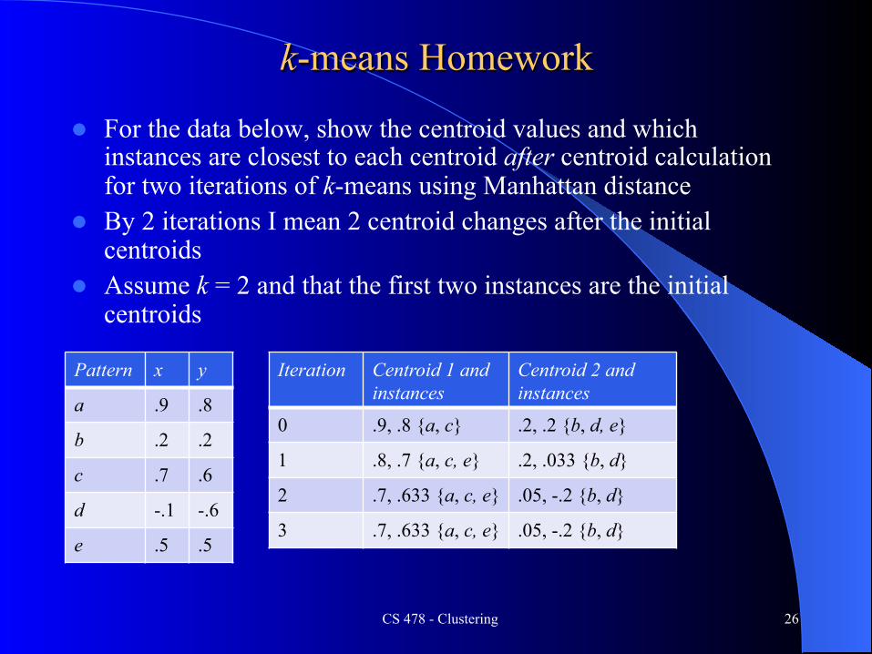
l  For the data below, show the centroid values and which instances are closest to each centroid after centroid calculation for two iterations of k-means using Manhattan distance

l  By 2 iterations I mean 2 centroid changes after the initial centroids

l  Assume k = 2 and that the first two instances are the initial centroids


Pattern x y

a .9 .8

b .2 .2

c .7 .6

d -.1 -.6

e .5 .5

Iteration Centroid 1 and instances

Centroid 2 and instances

0 .9, .8 {a, c} .2, .2 {b, d, e}

1 .8, .7 {a, c, e} .2, .033 {b, d}

2 .7, .633 {a, c, e} .05, -.2 {b, d}

3 .7, .633 {a, c, e} .05, -.2 {b, d}

Perceptron Homework - axon.cs.byu.edu

Documents

Transcript of Perceptron Homework - axon.cs.byu.edu