Multilayer Perceptron and Deep Learning - uni-goettingen.de · Supervised learning Multilayer...
69
Supervised learning Multilayer Perceptron and Deep Learning Some slides are adopted from Honglak Lee, Geoffrey Hinton, Yann LeCun and Marc'Aurelio Ranzato
Transcript of Multilayer Perceptron and Deep Learning - uni-goettingen.de · Supervised learning Multilayer...
Supervised learning
Multilayer Perceptron and
Deep Learning
Some slides are adopted from Honglak Lee, Geoffrey Hinton, Yann LeCun and Marc'Aurelio Ranzato
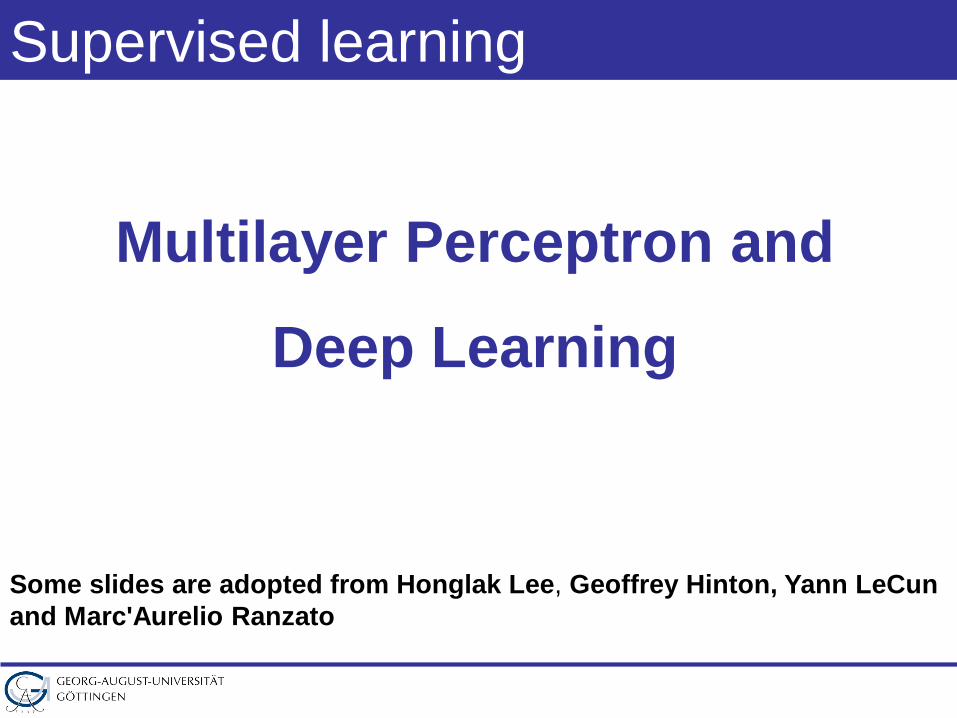
Threshold Logic Unit (TLU)
u2 Σ
u1
un
...
w1
w2
wna=Σi=1
n wi ui
v
inputsweights
activation output
θ
1 if a ≥ θv=
0 if a < θ{
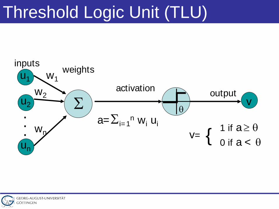
Example: Logical AND and OR
u1 u2 a v0 0 0 00 1 1 01 0 1 01 1 2 1
u1
u2
10
0 0
w1=1w2=1θ=1.5
u1
u2
11
0 1
w1=1w2=1θ=0.5
u1 u2 a v0 0 0 00 1 1 11 0 1 11 1 2 1
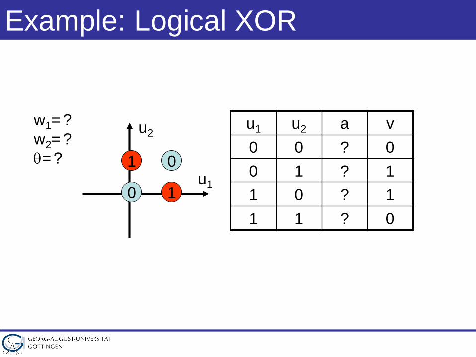
Example: Logical XOR
u1
u2
01
0 1
u1 u2 a v0 0 ? 00 1 ? 11 0 ? 11 1 ? 0
w1=?w2=?θ=?
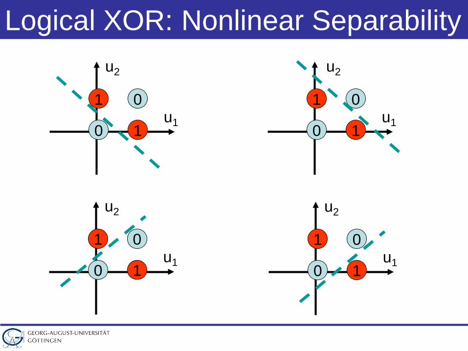
Logical XOR: Nonlinear Separability
u1
u2
01
0 1u1
u2
01
0 1
u1
u2
01
0 1u1
u2
01
0 1
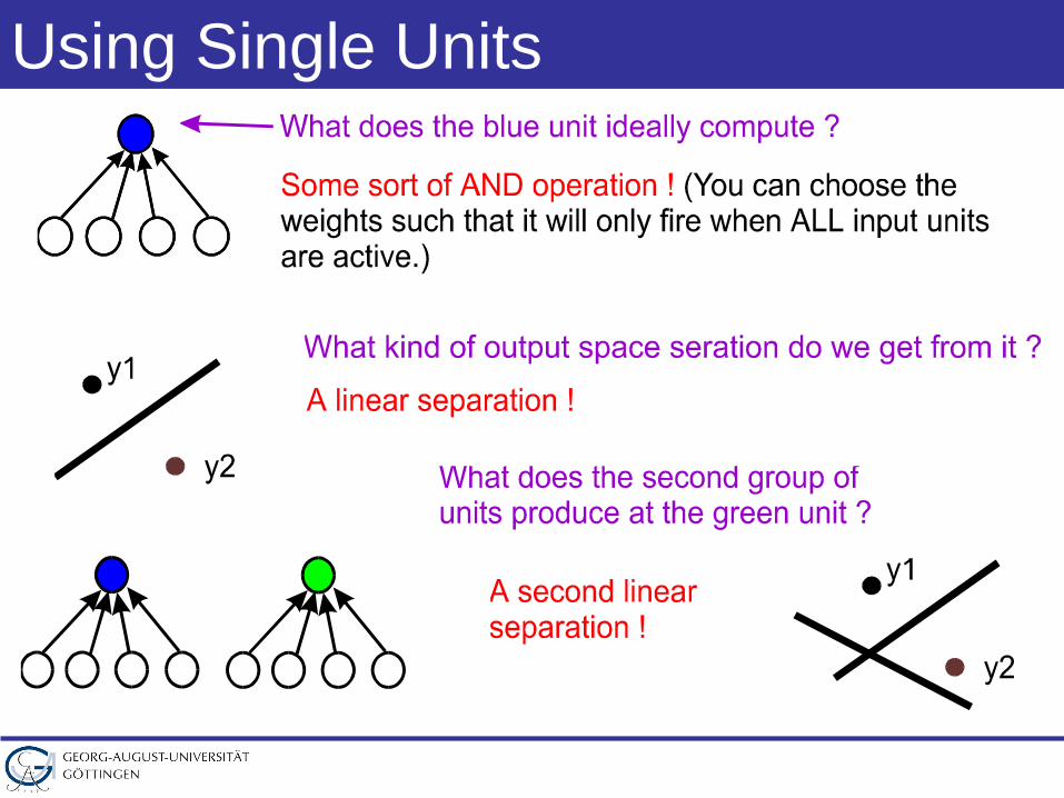
Using Single Units
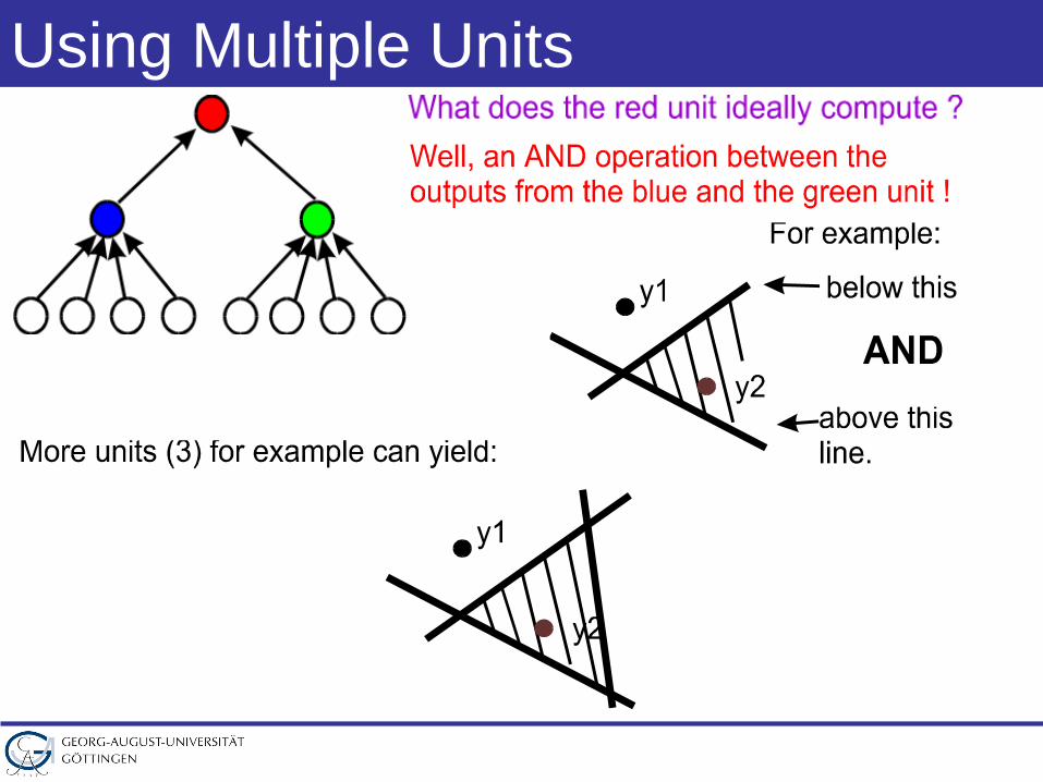
Using Multiple Units
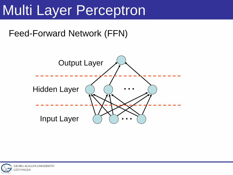
Multi Layer Perceptron
…
…
Feed-Forward Network (FFN)
Output Layer
Hidden Layer
Input Layer
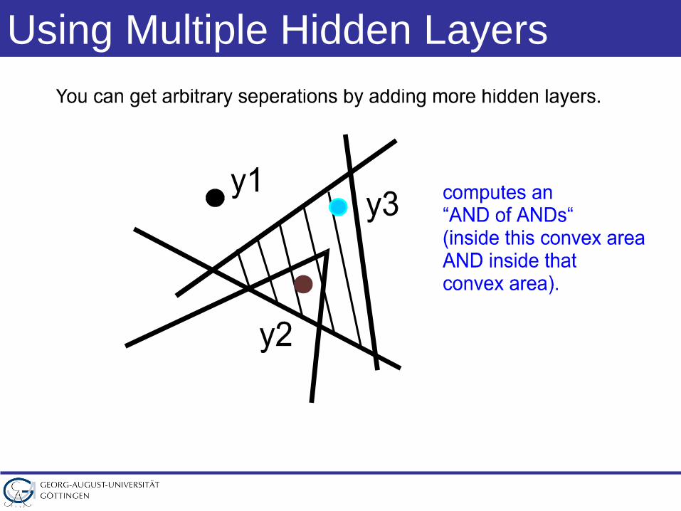
Using Multiple Hidden Layers
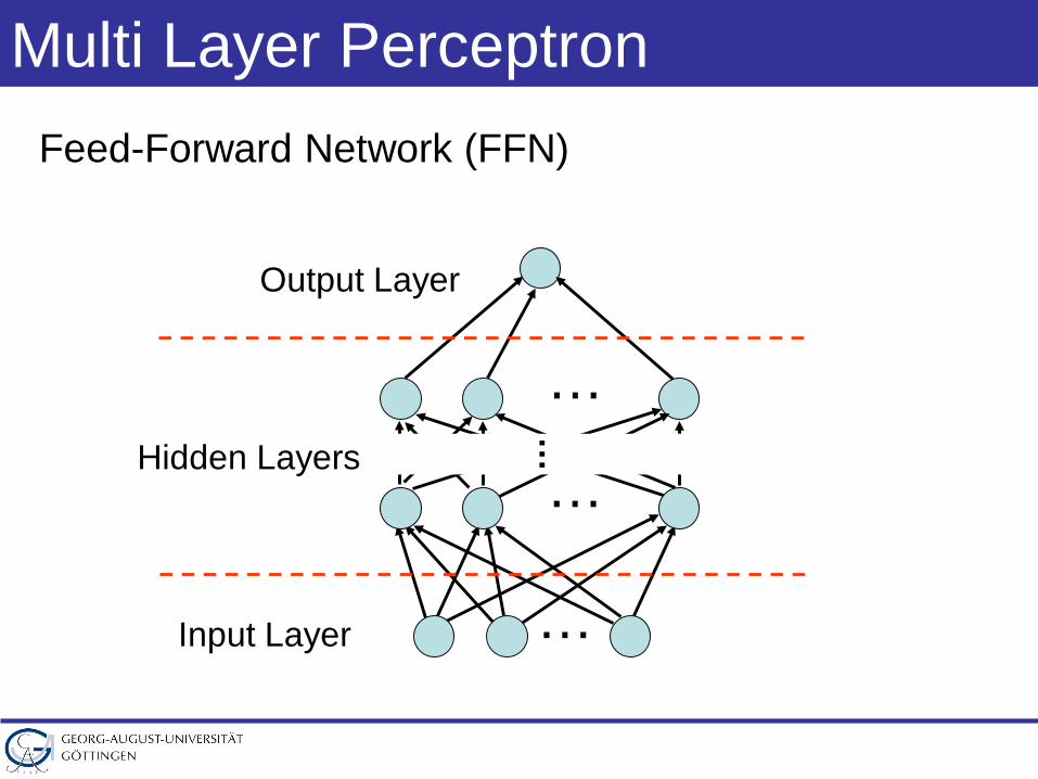
Multi Layer Perceptron
…
…
Feed-Forward Network (FFN)
Output Layer
Hidden Layers
Input Layer
……
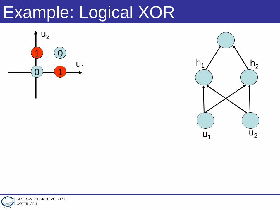
Example: Logical XOR
u1
u2
01
0 1
u1 u2
h1 h2
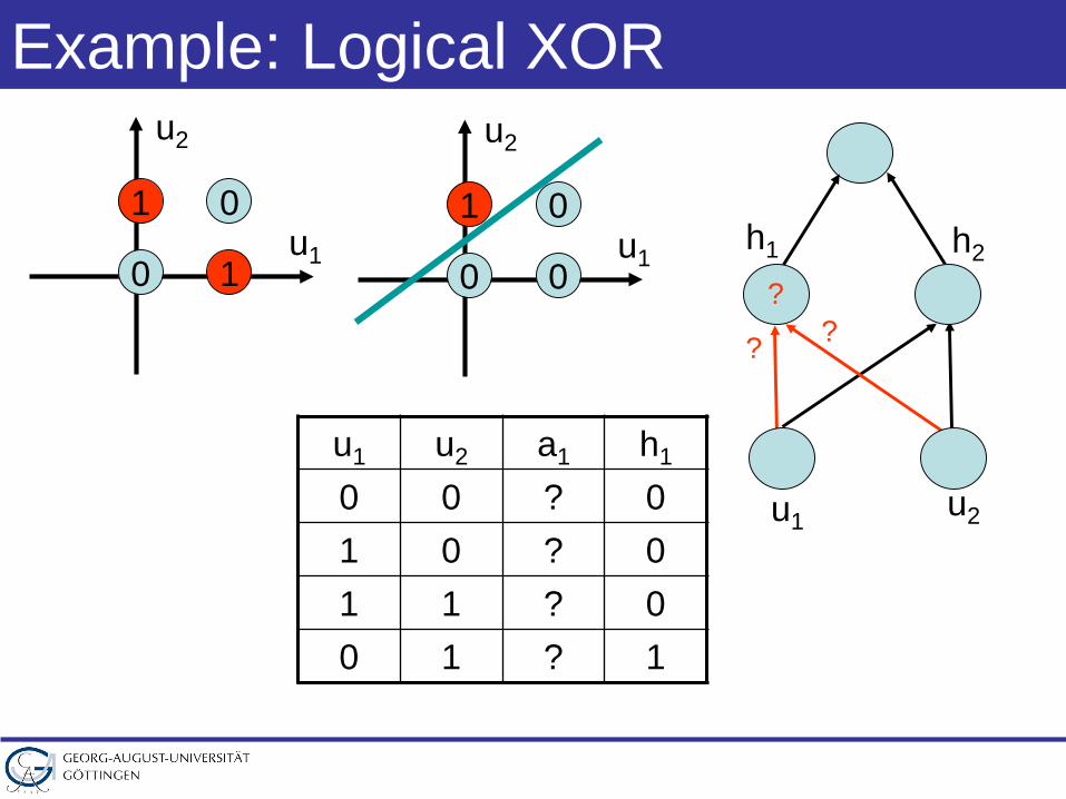
Example: Logical XOR
u1
u2
01
0 1
u1 u2
u1
u2
01
0 0
? ??
h1 h2
u1 u2 a1 h1
0 0 ? 01 0 ? 01 1 ? 00 1 ? 1
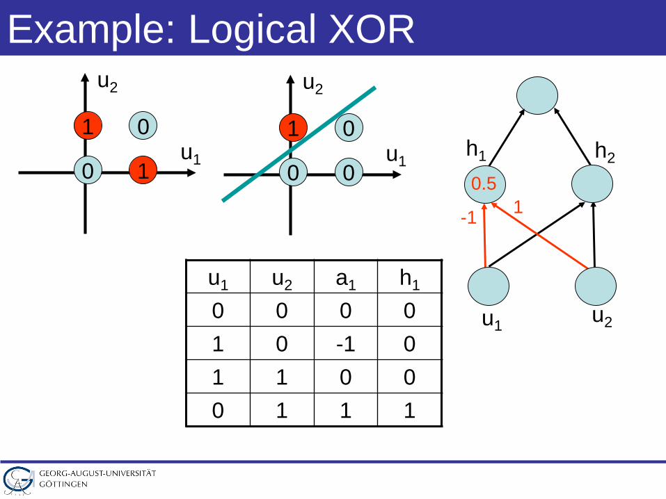
Example: Logical XOR
u1
u2
01
0 1
u1 u2
u1
u2
01
0 0
-1 10.5
h1 h2
u1 u2 a1 h1
0 0 0 01 0 -1 01 1 0 00 1 1 1
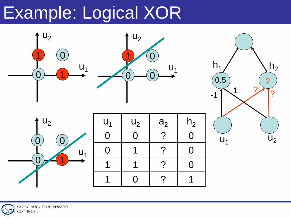
Example: Logical XOR
u1
u2
01
0 1
u1 u2
u1
u2
01
0 0
-1 10.5
u1
u2
00
0 1
? ??
h1 h2
u1 u2 a2 h2
0 0 ? 00 1 ? 01 1 ? 01 0 ? 1
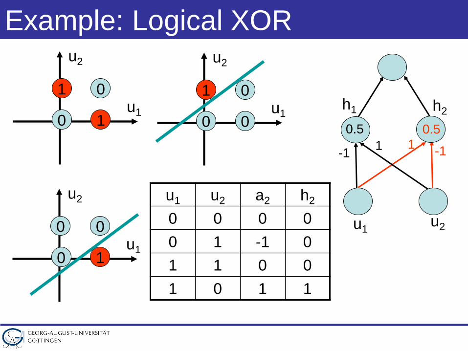
Example: Logical XOR
u1
u2
01
0 1
u1 u2
u1
u2
01
0 0
-1 10.5
u1
u2
00
0 1
1 -1
0.5
h1 h2
u1 u2 a2 h2
0 0 0 00 1 -1 01 1 0 01 0 1 1
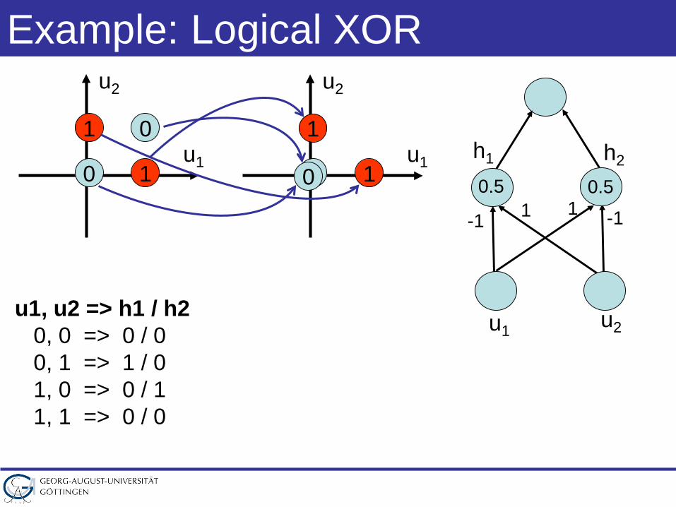
Example: Logical XOR
u1
u2
01
0 1
u1 u2
-1 10.5
1 -1
0.5
h1 h2
u1, u2 => h1 / h20, 0 => 0 / 00, 1 => 1 / 01, 0 => 0 / 11, 1 => 0 / 0
u1
u2
1
0 10
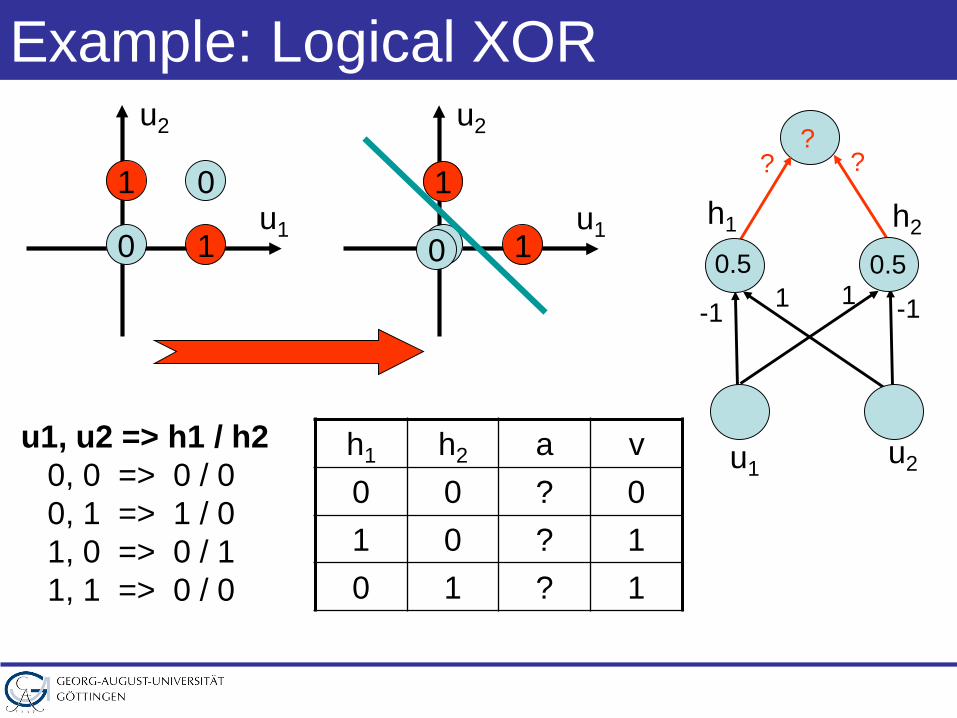
Example: Logical XOR
u1
u2
01
0 1
u1, u2 => h1 / h20, 0 => 0 / 00, 1 => 1 / 01, 0 => 0 / 11, 1 => 0 / 0
u1
u2
1
0 10
h1 h2 a v0 0 ? 01 0 ? 10 1 ? 1
u1 u2
-1 10.5
1 -1
0.5
h1 h2
? ??
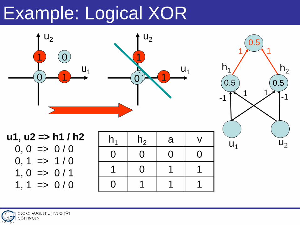
Example: Logical XOR
u1
u2
01
0 1
u1, u2 => h1 / h20, 0 => 0 / 00, 1 => 1 / 01, 0 => 0 / 11, 1 => 0 / 0
u1
u2
1
0 10
h1 h2 a v0 0 0 01 0 1 10 1 1 1
u1 u2
-1 10.5
1 -1
0.5
h1 h2
1 10.5
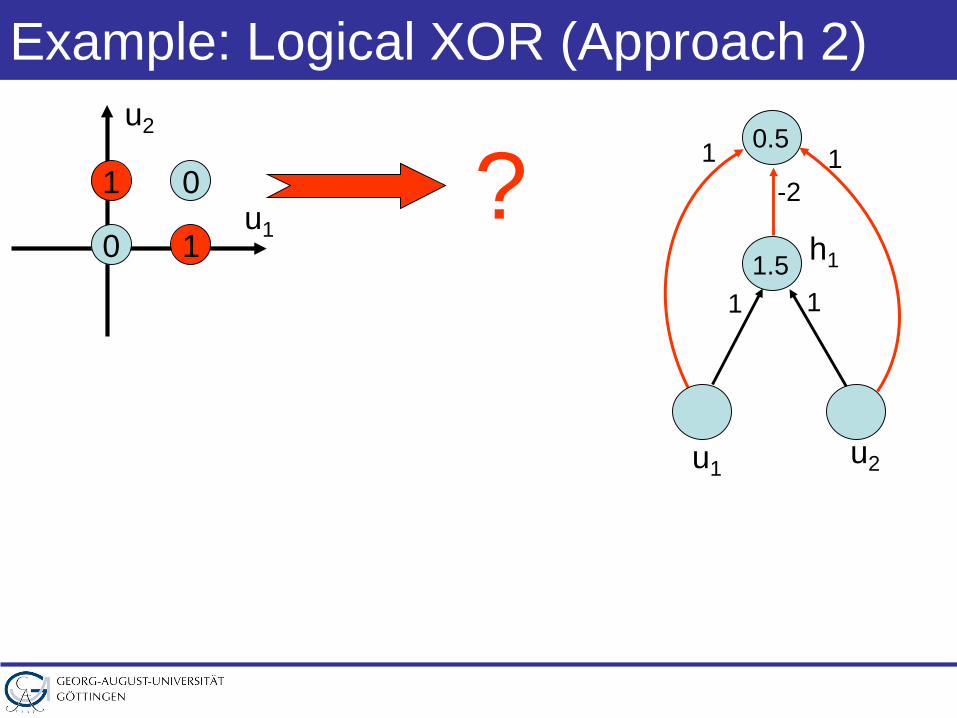
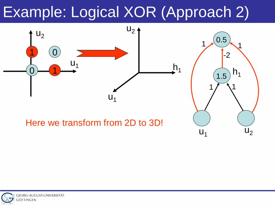
Example: Logical XOR (Approach 2)
u1
u2
01
0 1
u1 u2
11.5
1
1
h1
1-2
0.5
?
Example: Logical XOR (Approach 2)
u1
u2
01
0 1
u1 u2
11.5
1
1
h1
1-2
0.5
u1
h1
u2
Here we transform from 2D to 3D!
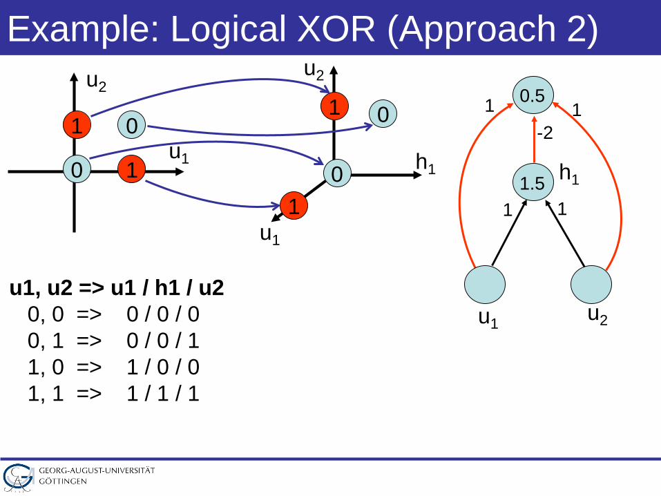
Example: Logical XOR (Approach 2)
u1
u2
01
0 1
u1 u2
11.5
1
1
h1
1-2
0.5
u1, u2 => u1 / h1 / u20, 0 => 0 / 0 / 00, 1 => 0 / 0 / 11, 0 => 1 / 0 / 01, 1 => 1 / 1 / 1
u1
h1
u2
0
01
1
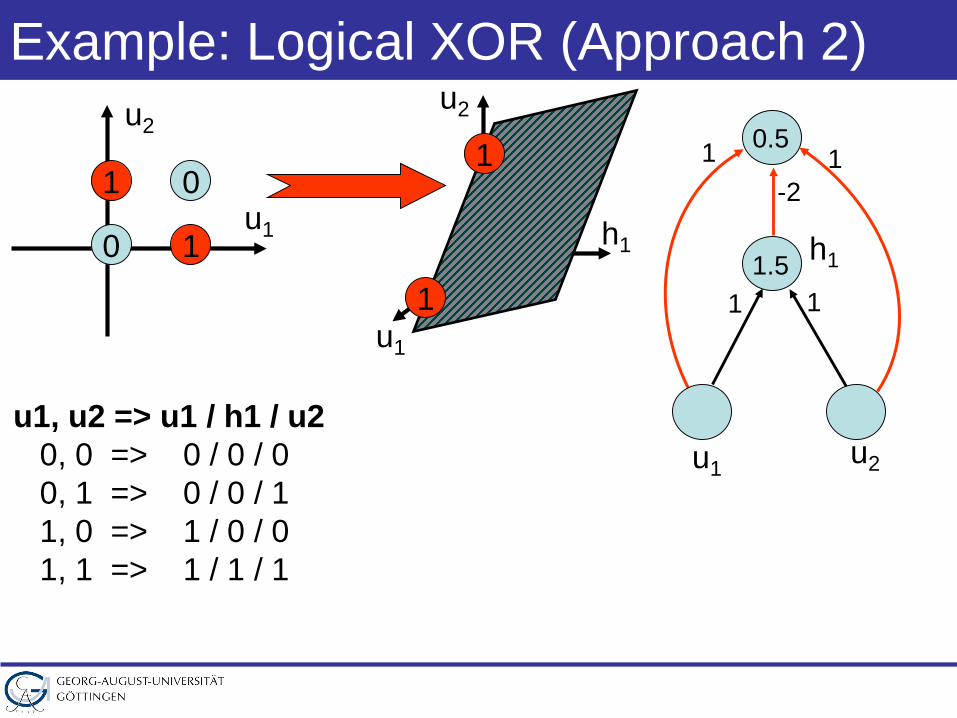
Example: Logical XOR (Approach 2)
u1
u2
01
0 1
u1 u2
11.5
1
1
h1
1-2
0.5
u1, u2 => u1 / h1 / u20, 0 => 0 / 0 / 00, 1 => 0 / 0 / 11, 0 => 1 / 0 / 01, 1 => 1 / 1 / 1
u1
h1
u2
0
01
1
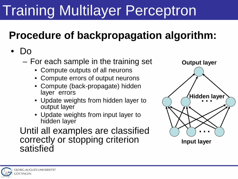
Training Multilayer Perceptron
• Do– For each sample in the training set
• Compute outputs of all neurons• Compute errors of output neurons• Compute (back-propagate) hidden
layer errors• Update weights from hidden layer to
output layer• Update weights from input layer to
hidden layerUntil all examples are classified correctly or stopping criterion satisfied
Procedure of backpropagation algorithm:
…
…Input layer
Output layer
Hidden layer
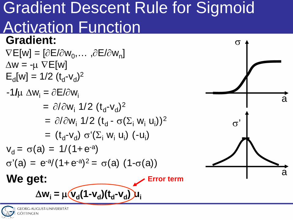
Gradient:∇E[w] = [∂E/∂w0,… ,∂E/∂wn]∆w = -µ ∇E[w]Ed[w] = 1/2 (td-vd)2
Gradient Descent Rule for Sigmoid Activation Function
a
σ
a
σ’
-1/µ ∆wi = ∂E/∂wi
= ∂/∂wi 1/2 (td-vd)2
= ∂/∂wi 1/2 (td - σ(Σi wi ui))2
= (td-vd) σ‘(Σi wi ui) (-ui)vd = σ(a) = 1/(1+e-a)σ’(a) = e-a/(1+e-a)2 = σ(a) (1-σ(a))
We get:∆wi = µ vd(1-vd)(td-vd) ui
Error term
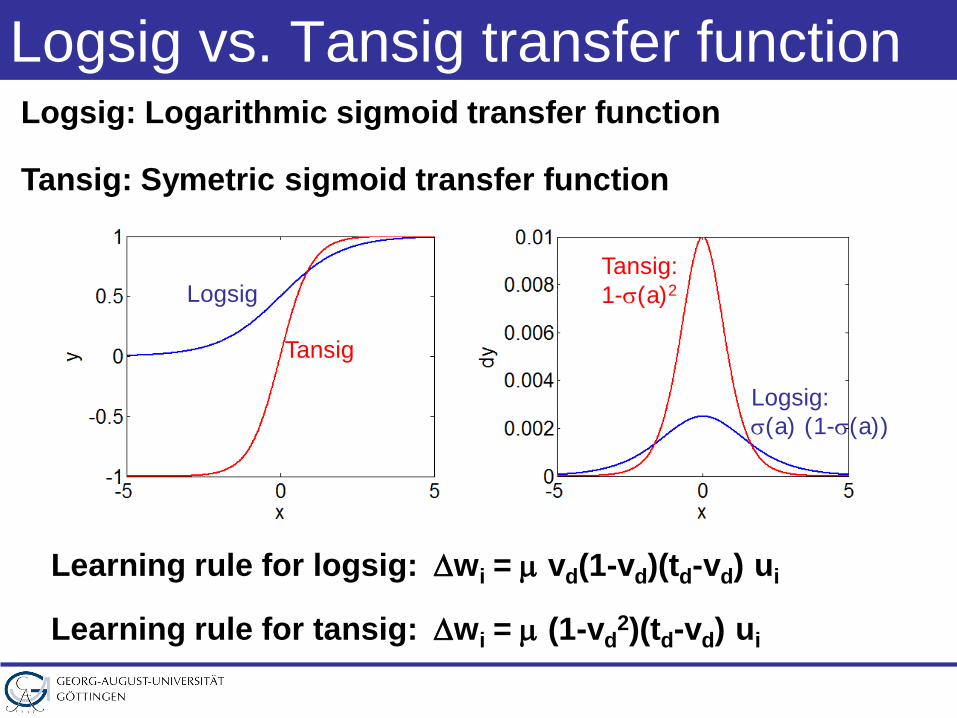
Logsig vs. Tansig transfer functionLogsig: Logarithmic sigmoid transfer function
Tansig: Symetric sigmoid transfer function
Logsig
Tansig
Logsig:σ(a) (1-σ(a))
Tansig:1-σ(a)2
Learning rule for logsig: ∆wi = µ vd(1-vd)(td-vd) ui
Learning rule for tansig: ∆wi = µ (1-vd2)(td-vd) ui
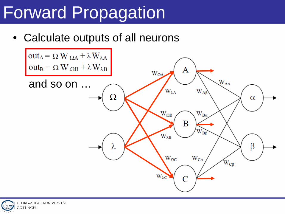
Forward Propagation• Calculate outputs of all neurons
and so on …
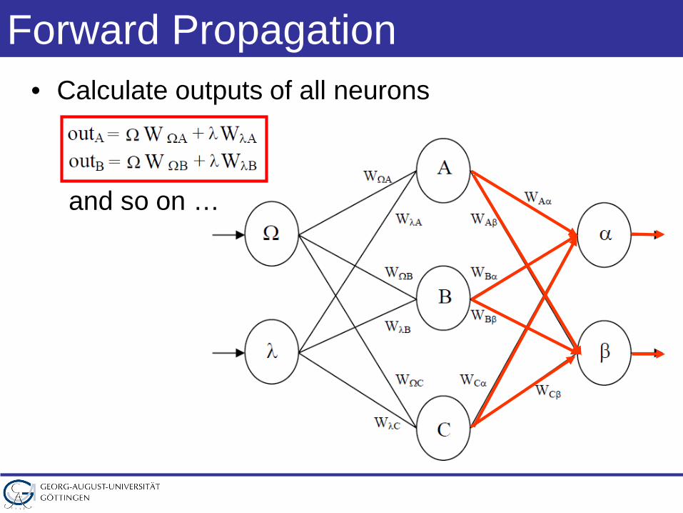
Forward Propagation• Calculate outputs of all neurons
and so on …
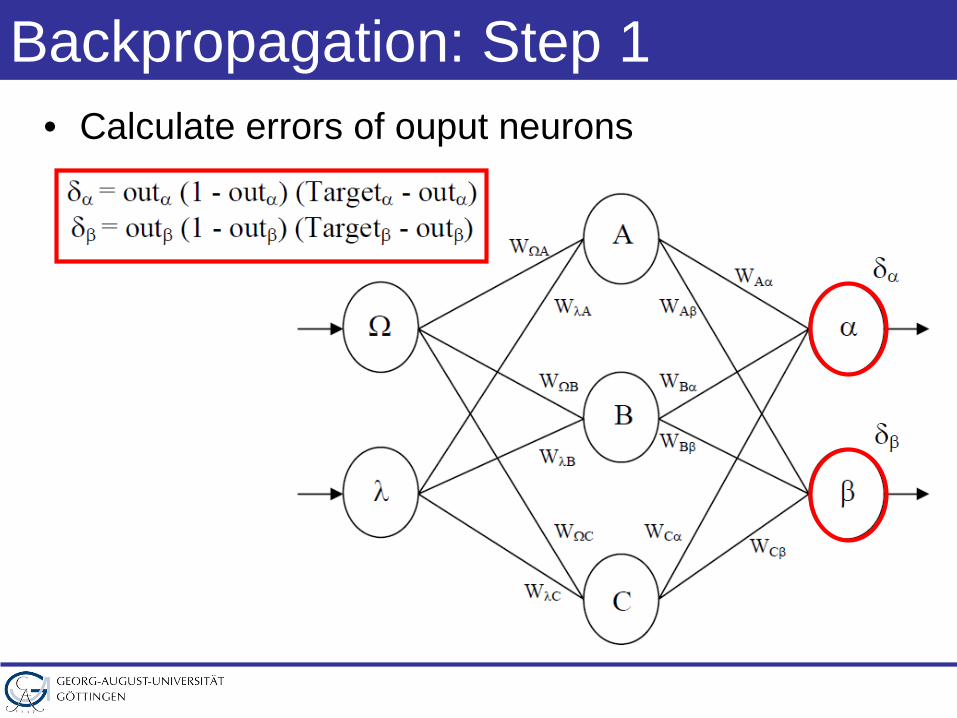
Backpropagation: Step 1• Calculate errors of ouput neurons
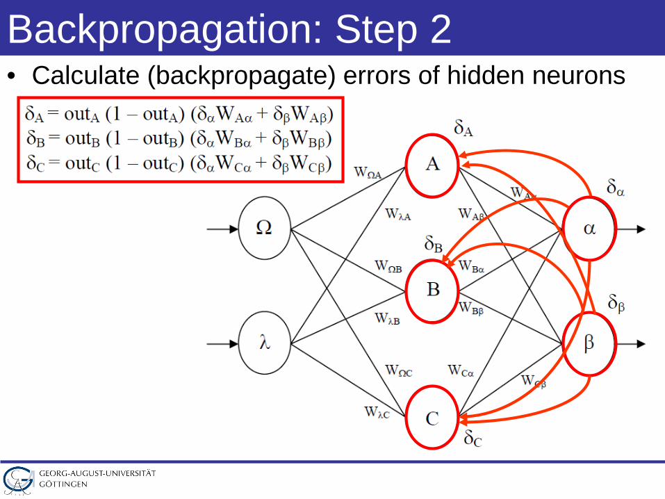
Backpropagation: Step 2• Calculate (backpropagate) errors of hidden neurons
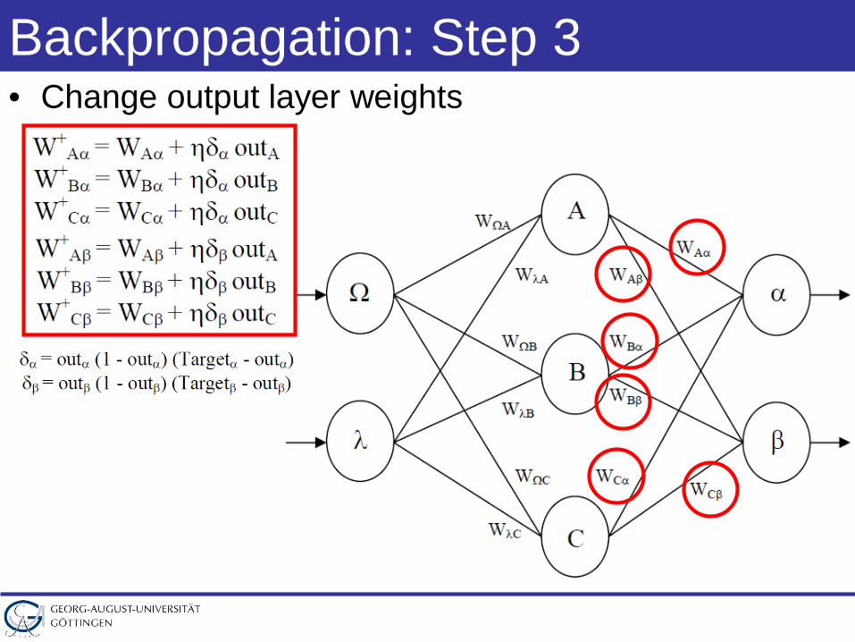
Backpropagation: Step 3• Change output layer weights
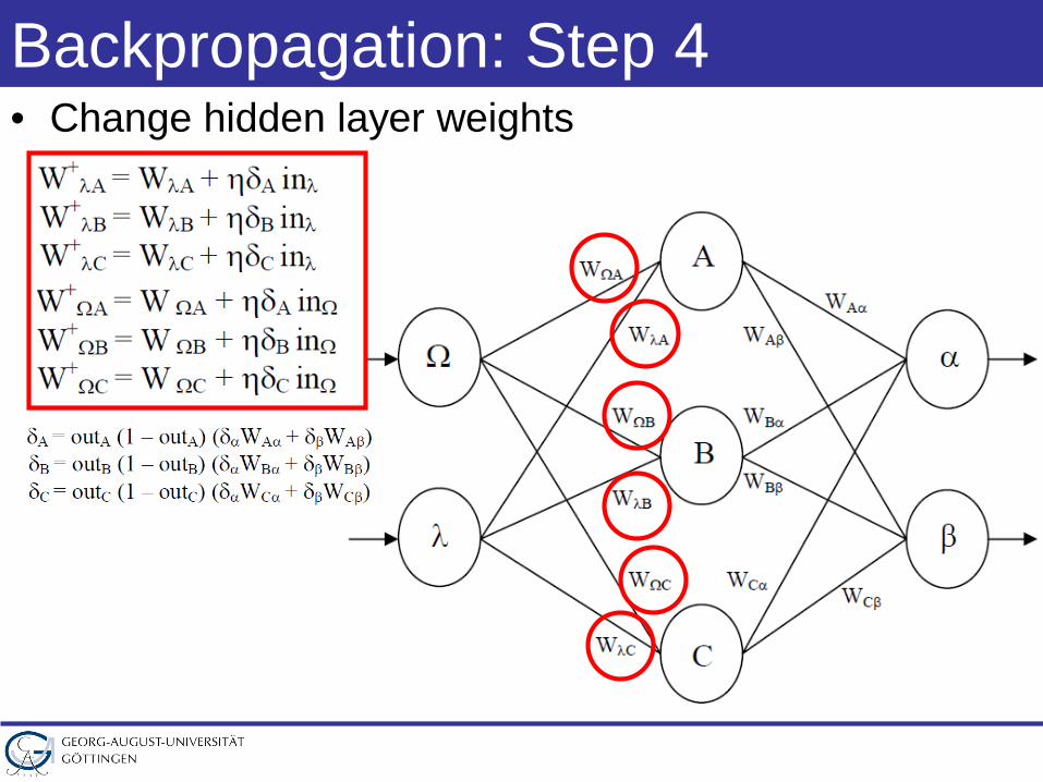
Backpropagation: Step 4• Change hidden layer weights
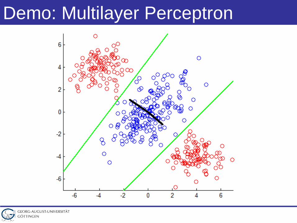
Demo: Multilayer Perceptron
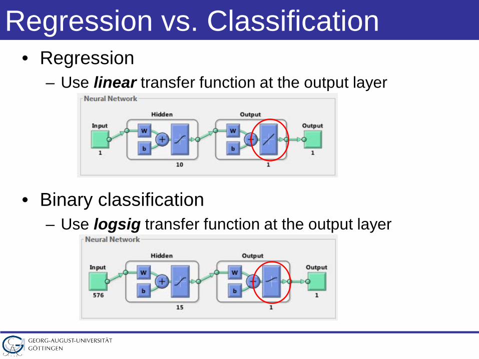
Regression vs. Classification• Regression
– Use linear transfer function at the output layer
• Binary classification– Use logsig transfer function at the output layer
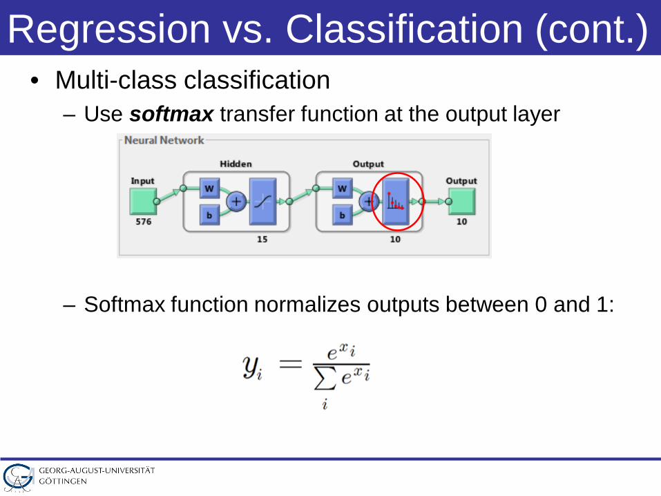
Regression vs. Classification (cont.)• Multi-class classification
– Use softmax transfer function at the output layer
– Softmax function normalizes outputs between 0 and 1:
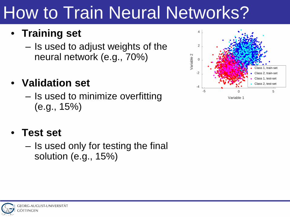
How to Train Neural Networks?• Training set
– Is used to adjust weights of the neural network (e.g., 70%)
• Validation set– Is used to minimize overfitting
(e.g., 15%)
• Test set– Is used only for testing the final
solution (e.g., 15%)
-5 0 5
Variable 1
-4
-2
0
2
4
Var
iabl
e 2
Class 1, train-set
Class 2, train-set
Class 1, test-set
Class 2, test-set
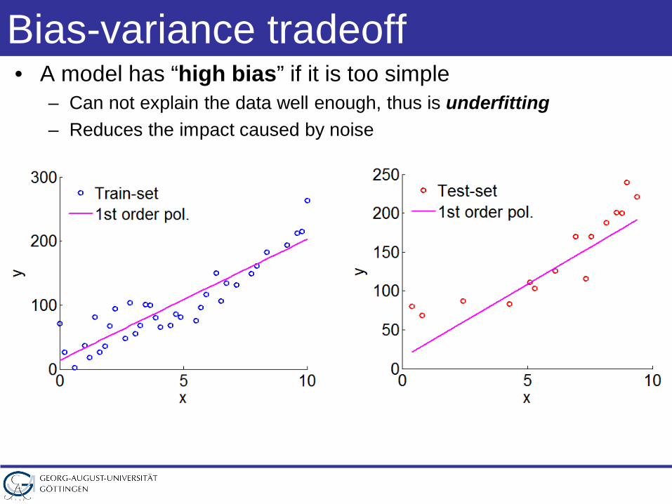
Bias-variance tradeoff• A model has “high bias” if it is too simple
– Can not explain the data well enough, thus is underfitting– Reduces the impact caused by noise
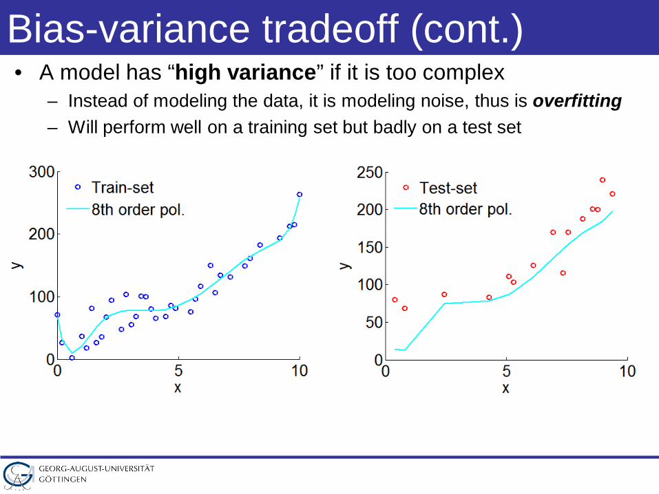
Bias-variance tradeoff (cont.)• A model has “high variance” if it is too complex
– Instead of modeling the data, it is modeling noise, thus is overfitting– Will perform well on a training set but badly on a test set
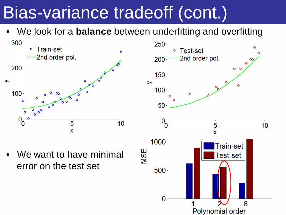
Bias-variance tradeoff (cont.)• We look for a balance between underfitting and overfitting
• We want to have minimalerror on the test set
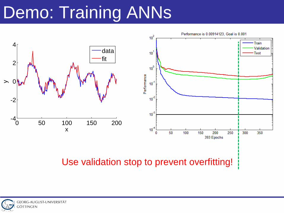
Demo: Training ANNs
0 50 100 150 200-4
-2
0
2
4
x
y
datafit
Use validation stop to prevent overfitting!
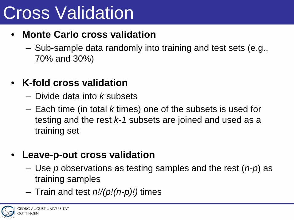
Cross Validation• Monte Carlo cross validation
– Sub-sample data randomly into training and test sets (e.g., 70% and 30%)
• K-fold cross validation– Divide data into k subsets– Each time (in total k times) one of the subsets is used for
testing and the rest k-1 subsets are joined and used as a training set
• Leave-p-out cross validation– Use p observations as testing samples and the rest (n-p) as
training samples– Train and test n!/(p!(n-p)!) times
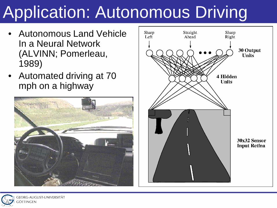
Application: Autonomous Driving• Autonomous Land Vehicle
In a Neural Network (ALVINN; Pomerleau, 1989)
• Automated driving at 70 mph on a highway
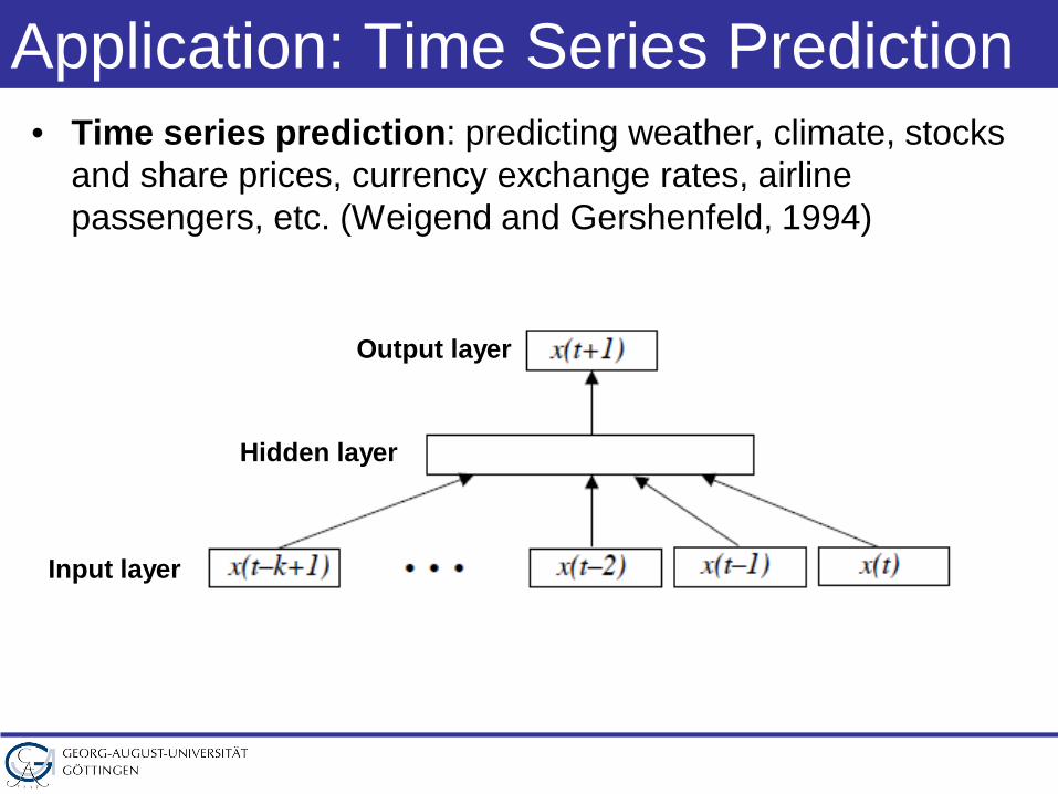
Application: Time Series Prediction• Time series prediction: predicting weather, climate, stocks
and share prices, currency exchange rates, airline passengers, etc. (Weigend and Gershenfeld, 1994)
Input layer
Hidden layer
Output layer
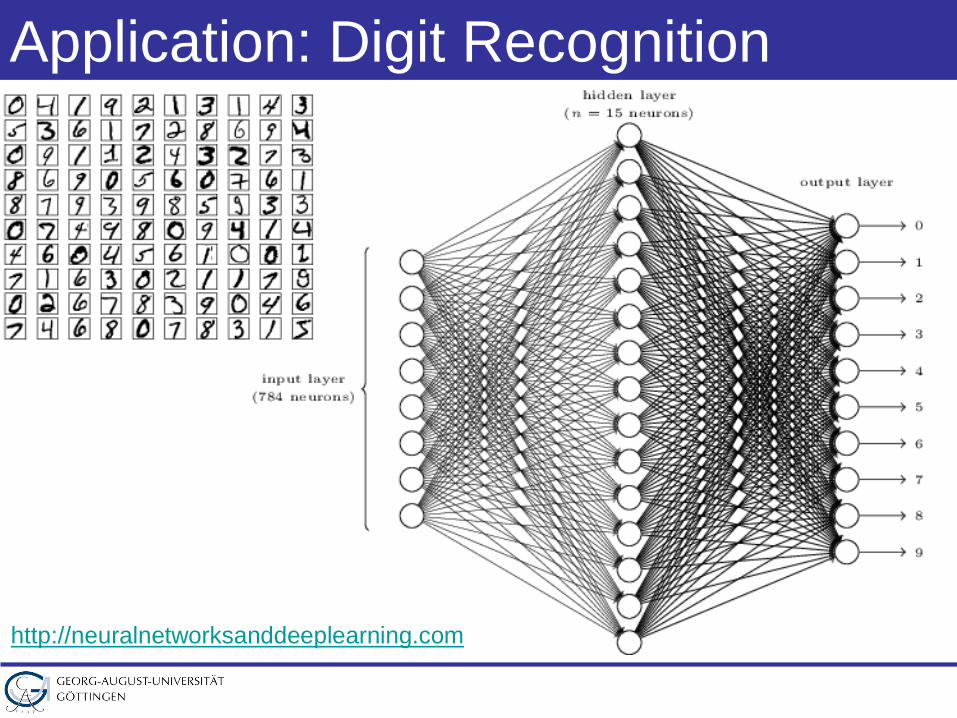
Application: Digit Recognition
http://neuralnetworksanddeeplearning.com
Supervised Learning
Deep Neural Networks
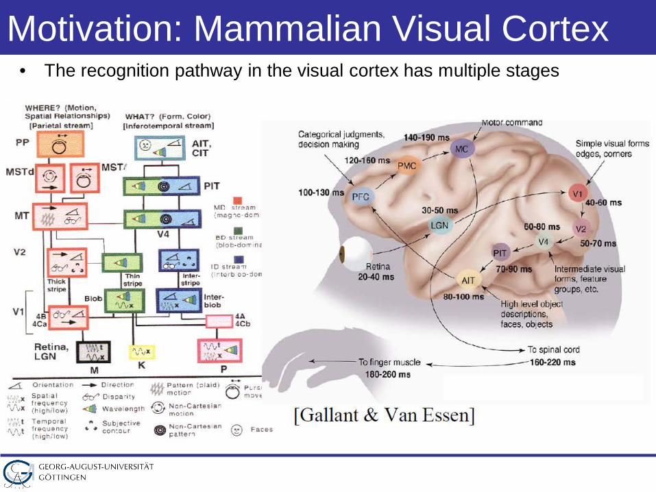
Motivation: Mammalian Visual Cortex• The recognition pathway in the visual cortex has multiple stages
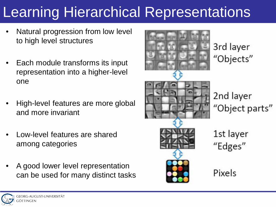
Learning Hierarchical Representations• Natural progression from low level
to high level structures
• Each module transforms its input representation into a higher-level one
• High-level features are more global and more invariant
• Low-level features are shared among categories
• A good lower level representation can be used for many distinct tasks
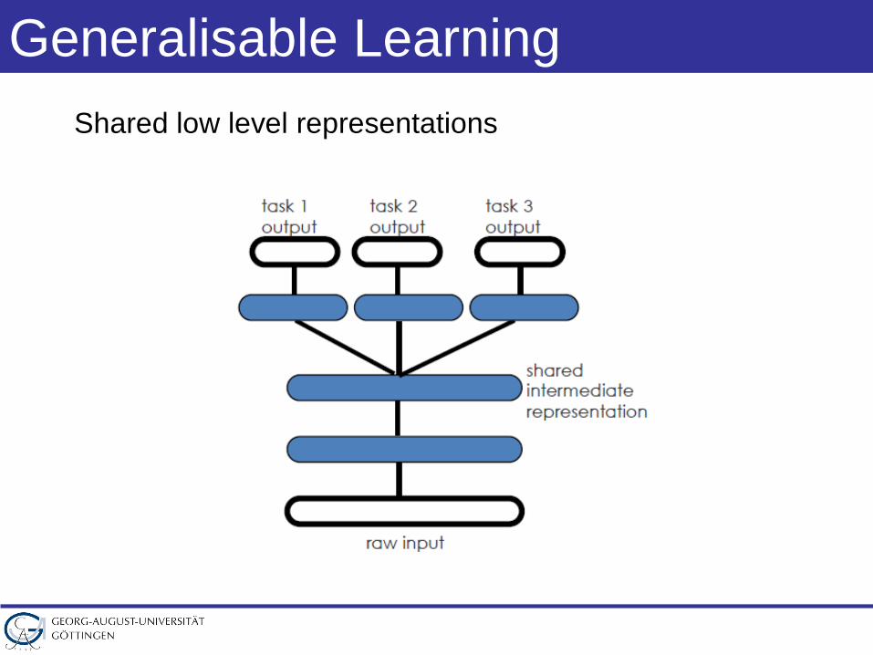
Generalisable LearningShared low level representations
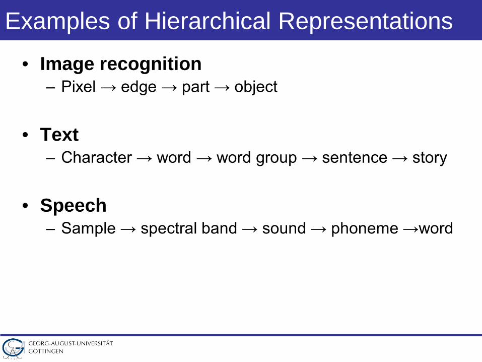
Examples of Hierarchical Representations
• Image recognition– Pixel → edge → part → object
• Text– Character → word → word group → sentence → story
• Speech– Sample → spectral band → sound → phoneme →word
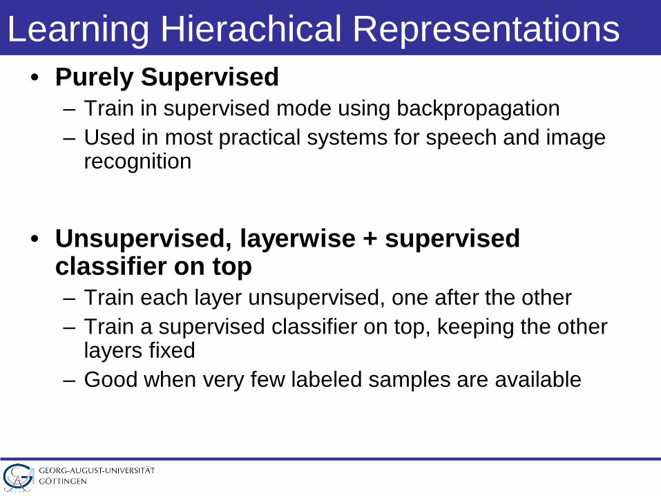
Learning Hierachical Representations• Purely Supervised
– Train in supervised mode using backpropagation– Used in most practical systems for speech and image
recognition
• Unsupervised, layerwise + supervised classifier on top– Train each layer unsupervised, one after the other– Train a supervised classifier on top, keeping the other
layers fixed– Good when very few labeled samples are available
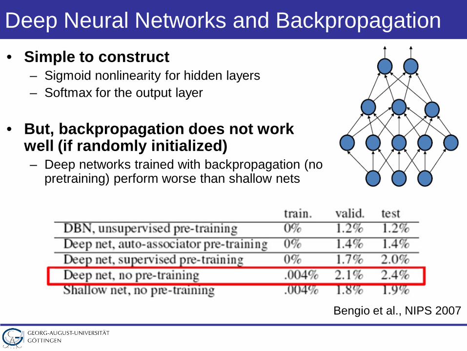
Deep Neural Networks and Backpropagation• Simple to construct
– Sigmoid nonlinearity for hidden layers– Softmax for the output layer
• But, backpropagation does not workwell (if randomly initialized) – Deep networks trained with backpropagation (no
pretraining) perform worse than shallow nets
Bengio et al., NIPS 2007
Problems with Backpropagation• Gradient is progressively getting more dilute
– Below top few layers, correction signal is minimal
– Gets stuck in local minima
– Especially if they start out far from ‘good’ regions (i.e., random initialization)
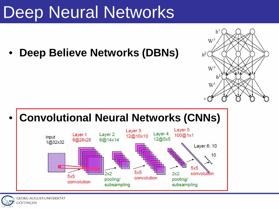
Deep Neural Networks
• Deep Believe Networks (DBNs)
• Convolutional Neural Networks (CNNs)
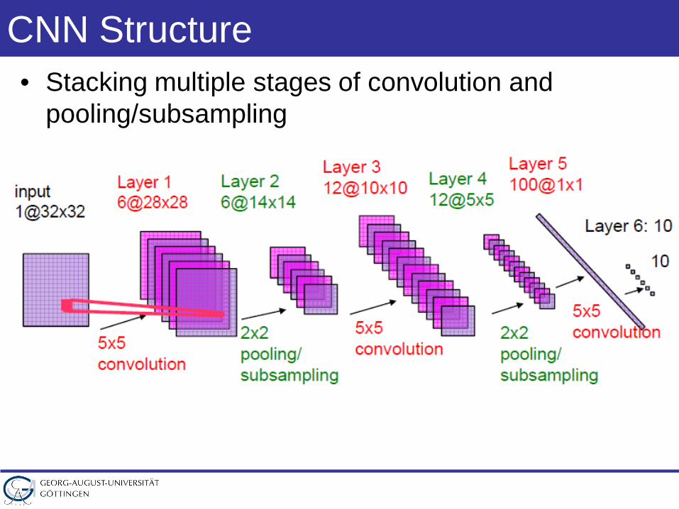
CNN Structure• Stacking multiple stages of convolution and
pooling/subsampling
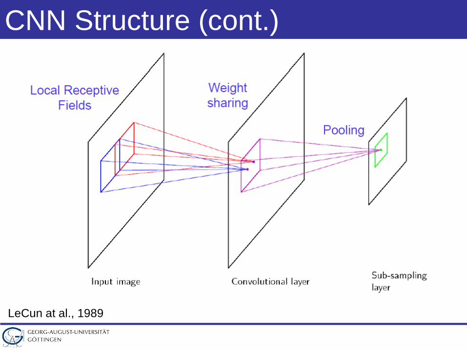
CNN Structure (cont.)
LeCun at al., 1989
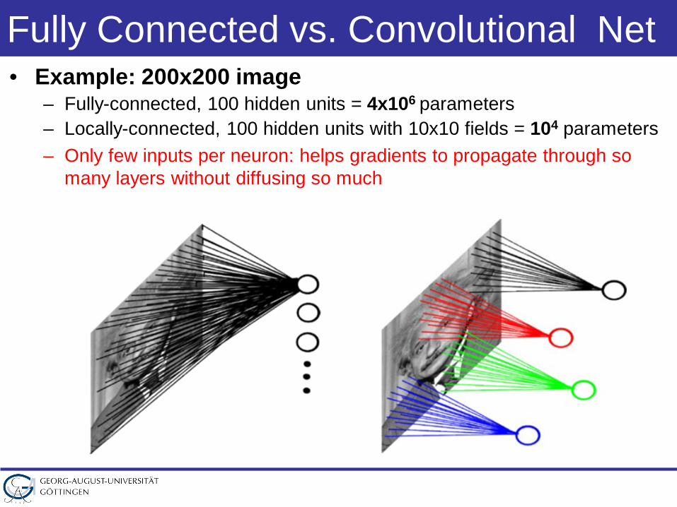
Fully Connected vs. Convolutional Net • Example: 200x200 image
– Fully-connected, 100 hidden units = 4x10⁶ parameters– Locally-connected, 100 hidden units with 10x10 fields = 104 parameters– Only few inputs per neuron: helps gradients to propagate through so
many layers without diffusing so much
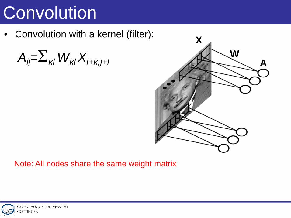
Convolution• Convolution with a kernel (filter):
AW
X
Aij=Σkl Wkl Xi+k,j+l
Note: All nodes share the same weight matrix
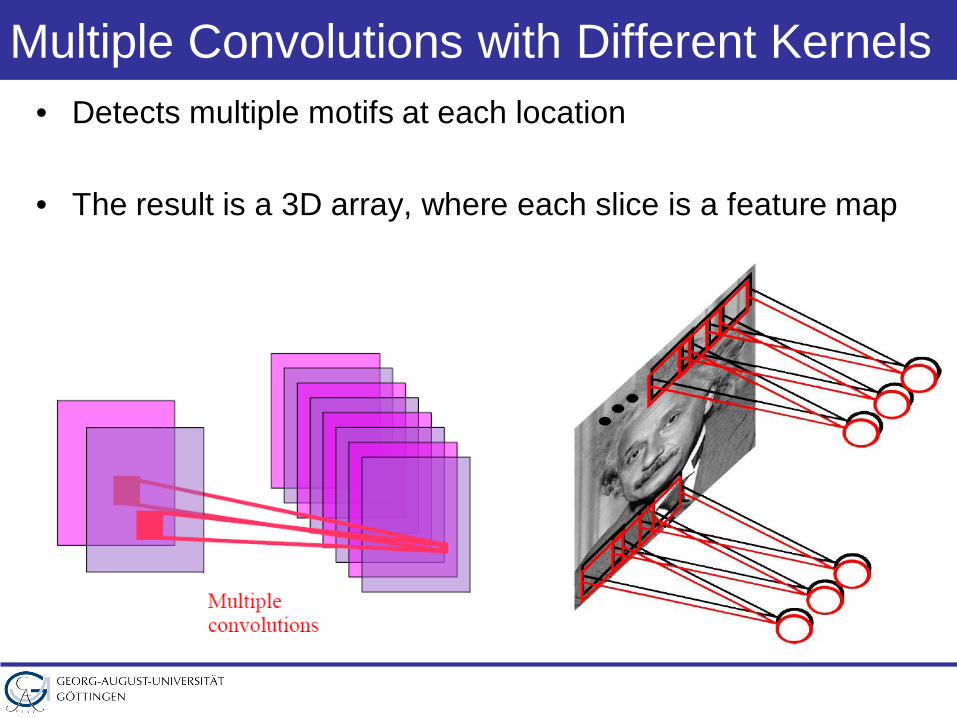
Multiple Convolutions with Different Kernels• Detects multiple motifs at each location
• The result is a 3D array, where each slice is a feature map
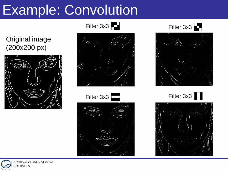
Example: Convolution
Original image(200x200 px)
Filter 3x3 Filter 3x3
Filter 3x3 Filter 3x3
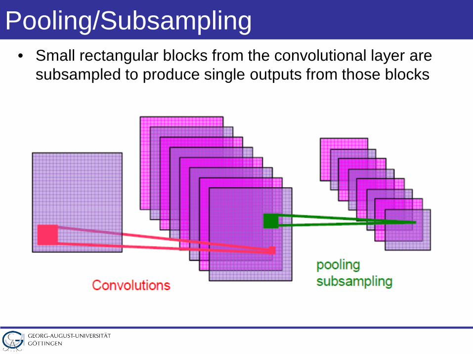
Pooling/Subsampling• Small rectangular blocks from the convolutional layer are
subsampled to produce single outputs from those blocks
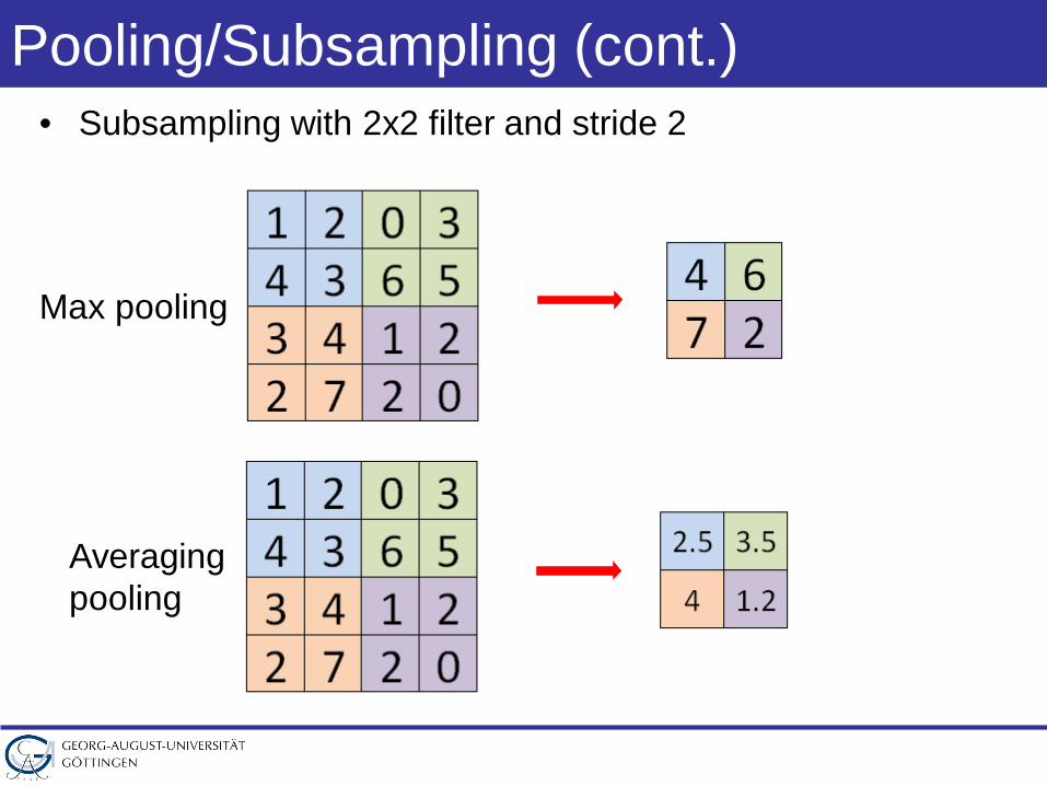
Pooling/Subsampling (cont.)• Subsampling with 2x2 filter and stride 2
Max pooling
Averagingpooling
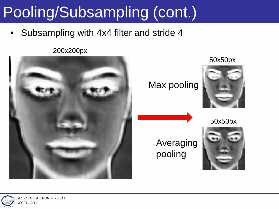
Pooling/Subsampling (cont.)• Subsampling with 4x4 filter and stride 4
200x200px50x50px
Max pooling
Averagingpooling
50x50px
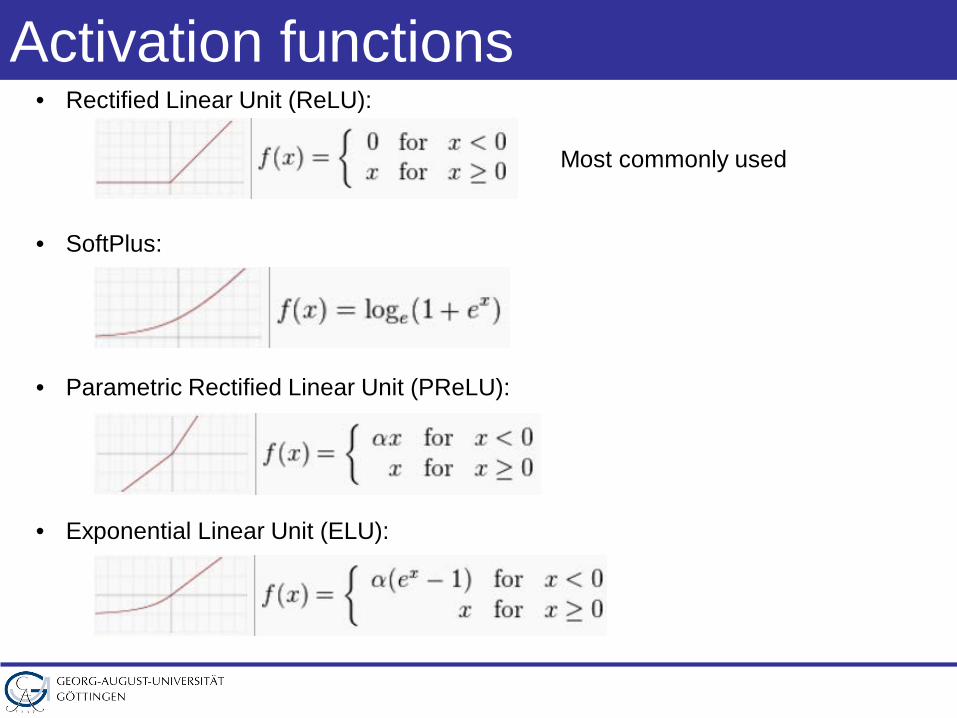
Activation functions• Rectified Linear Unit (ReLU):
• SoftPlus:
• Parametric Rectified Linear Unit (PReLU):
• Exponential Linear Unit (ELU):
Most commonly used
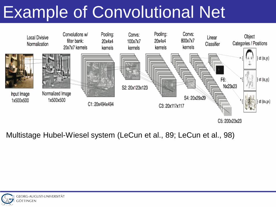
Example of Convolutional Net
Multistage Hubel-Wiesel system (LeCun et al., 89; LeCun et al., 98)
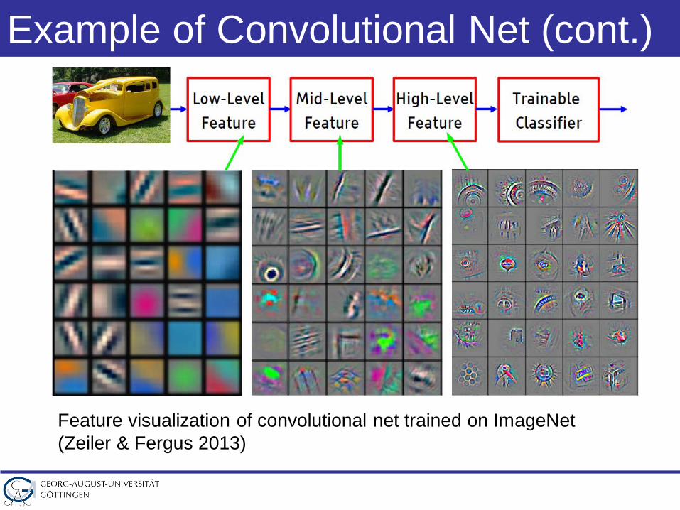
Example of Convolutional Net (cont.)
Feature visualization of convolutional net trained on ImageNet(Zeiler & Fergus 2013)
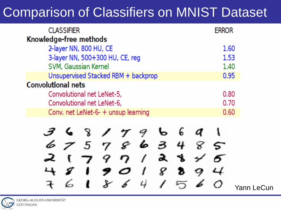
Comparison of Classifiers on MNIST Dataset
Yann LeCun
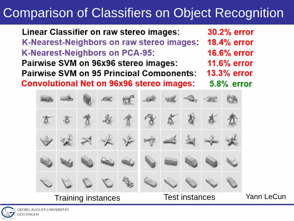
Comparison of Classifiers on Object Recognition
Yann LeCunTest instancesTraining instances
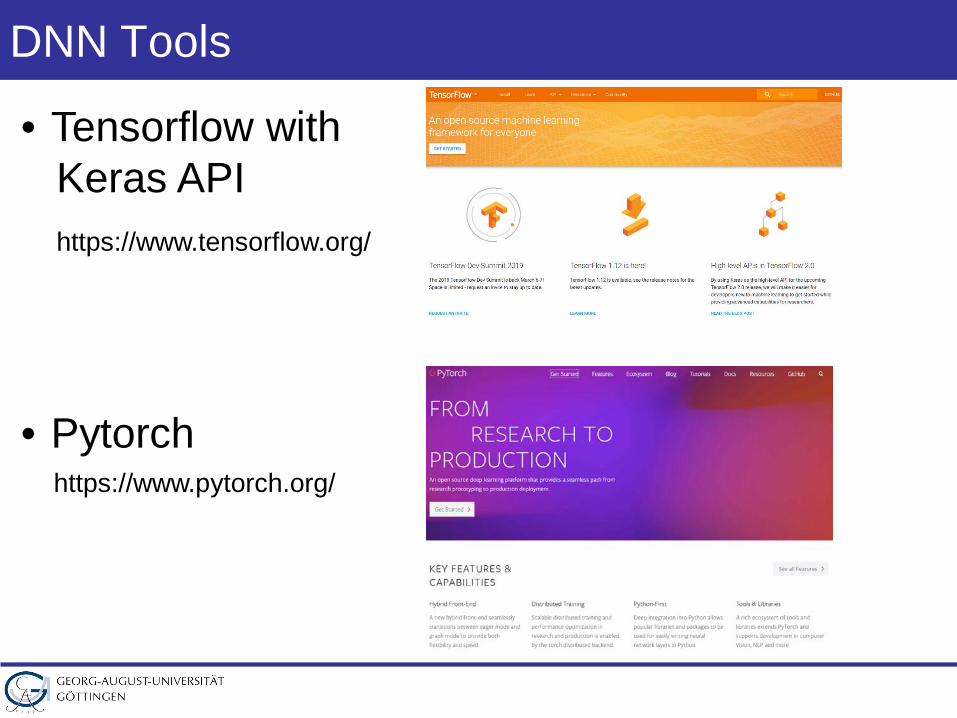
DNN Tools
• Tensorflow withKeras API
• Pytorchhttps://www.pytorch.org/
https://www.tensorflow.org/
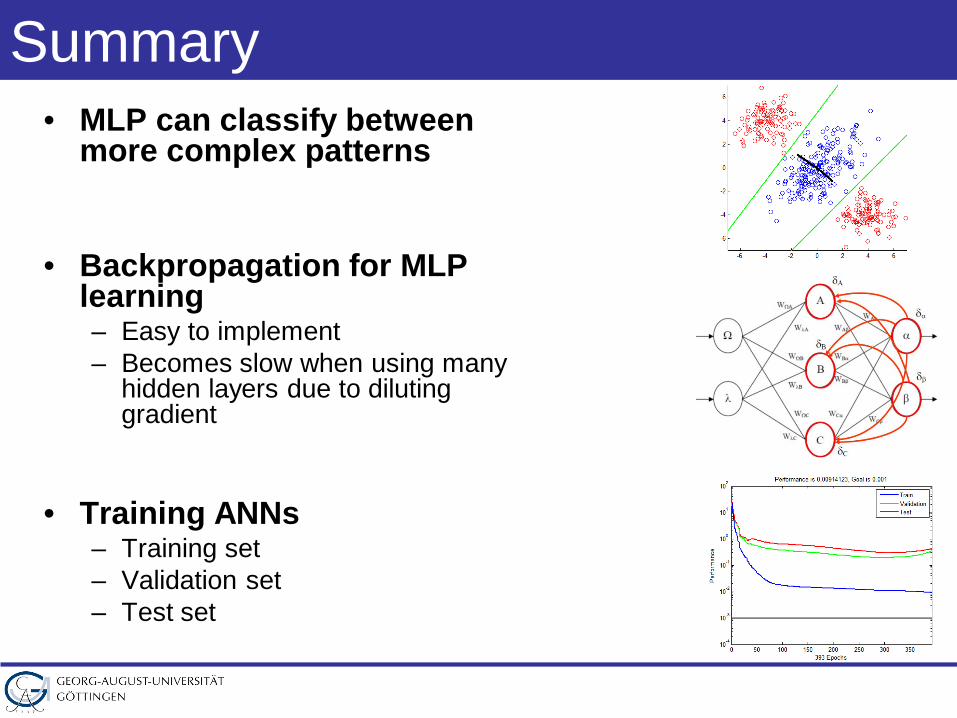
Summary• MLP can classify between
more complex patterns
• Backpropagation for MLP learning– Easy to implement– Becomes slow when using many
hidden layers due to diluting gradient
• Training ANNs– Training set– Validation set– Test set
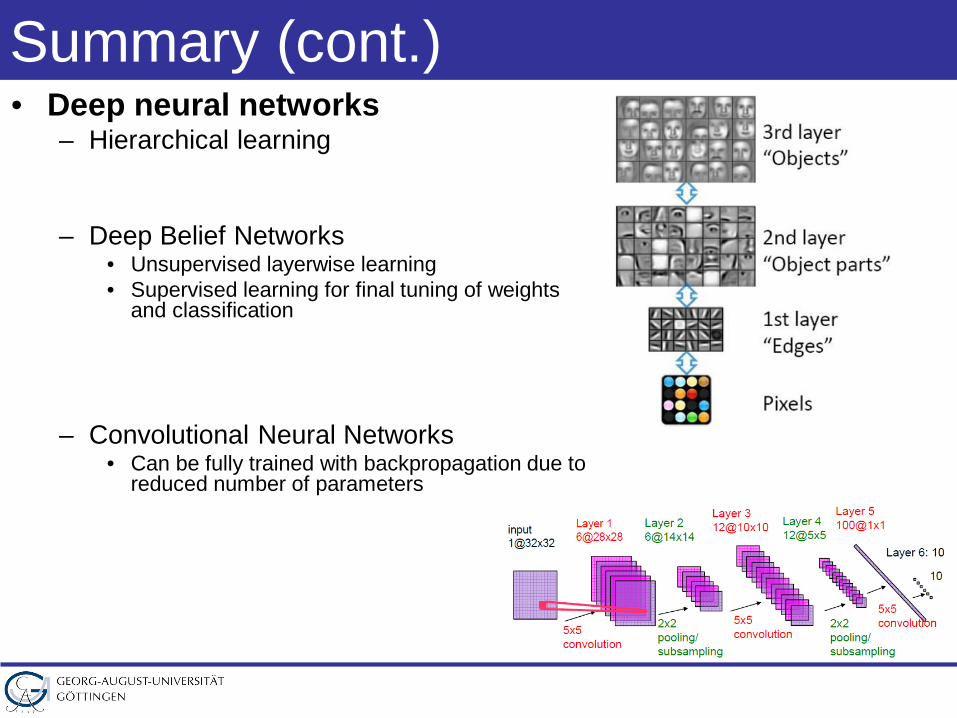
Summary (cont.)• Deep neural networks
– Hierarchical learning
– Deep Belief Networks• Unsupervised layerwise learning• Supervised learning for final tuning of weights
and classification
– Convolutional Neural Networks• Can be fully trained with backpropagation due to
reduced number of parameters