Particle size, charge, and flow - Colloidal 2005 Lecture 4 - Particulate size, charge, and flow 1...
34
ACS© 2005 Particle size, charge, and flow Lecture 4
Transcript of Particle size, charge, and flow - Colloidal 2005 Lecture 4 - Particulate size, charge, and flow 1...
ACS© 2005
Particle size, charge, and flow
Lecture 4
Lecture 4 - Particulate size, charge, and flow 1ACS© 2005
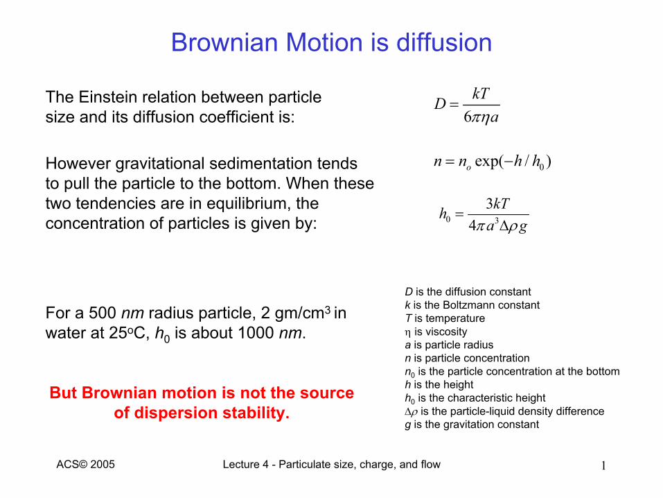
Brownian Motion is diffusion
6kTDaπη
=
0exp( / )on n h h= −
0 3
34
kTha gπ ρ
=∆
The Einstein relation between particle size and its diffusion coefficient is:
However gravitational sedimentation tends to pull the particle to the bottom. When these two tendencies are in equilibrium, the concentration of particles is given by:
For a 500 nm radius particle, 2 gm/cm3 in water at 25oC, h0 is about 1000 nm.
But Brownian motion is not the source of dispersion stability.
D is the diffusion constantk is the Boltzmann constantT is temperatureη is viscositya is particle radiusn is particle concentrationn0 is the particle concentration at the bottomh is the heighth0 is the characteristic height∆ρ is the particle-liquid density differenceg is the gravitation constant
Lecture 4 - Particulate size, charge, and flow 2ACS© 2005
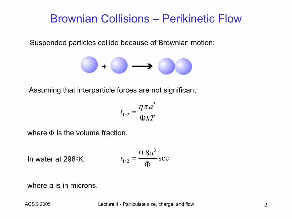
Brownian Collisions – Perikinetic Flow
3
1/ 2atkT
ηπ=Φ
3
1/ 20.8 secat =Φ
Suspended particles collide because of Brownian motion:
Assuming that interparticle forces are not significant:
where Φ is the volume fraction.
In water at 298oK:
where a is in microns.
Lecture 4 - Particulate size, charge, and flow 3ACS© 2005
Microscopy
Always look at particles in the microscope before doing any other type of size analysis!!
Microscope results are almost always the referee for a new technique.
Image analysis:
Reticle
Photograph
Digitized photograph
Digitized video
Electron microscopy
Orders of magnitude higher resolution
But samples are in vacuum at high temperature
Lecture 4 - Particulate size, charge, and flow 4ACS© 2005
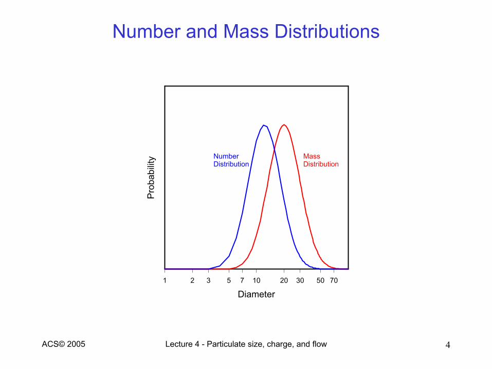
Number and Mass Distributions
Diameter1 2 3 5 7 10 20 30 50 70
Pro
babi
lity Number
DistributionMassDistribution
Lecture 4 - Particulate size, charge, and flow 5ACS© 2005
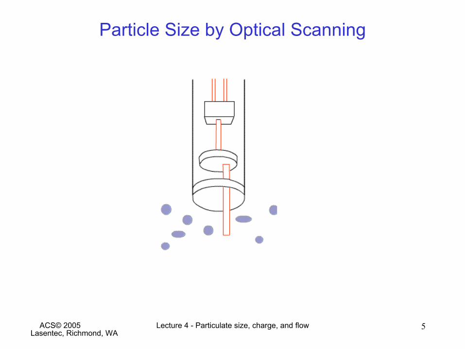
Particle Size by Optical Scanning
Lasentec, Richmond, WA
Lecture 4 - Particulate size, charge, and flow 6ACS© 2005
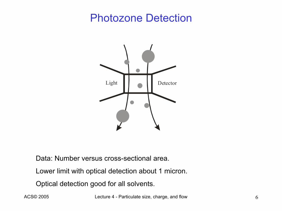
Photozone Detection
Data: Number versus cross-sectional area.
Lower limit with optical detection about 1 micron.
Optical detection good for all solvents.
Light Detector
Lecture 4 - Particulate size, charge, and flow 7ACS© 2005
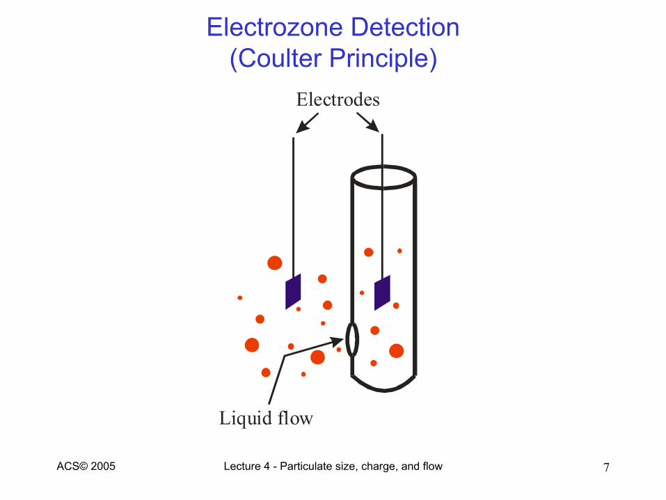
Electrozone Detection(Coulter Principle)
Electrodes
Liquid flow
Lecture 4 - Particulate size, charge, and flow 8ACS© 2005
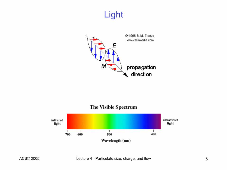
Light
Lecture 4 - Particulate size, charge, and flow 9ACS© 2005
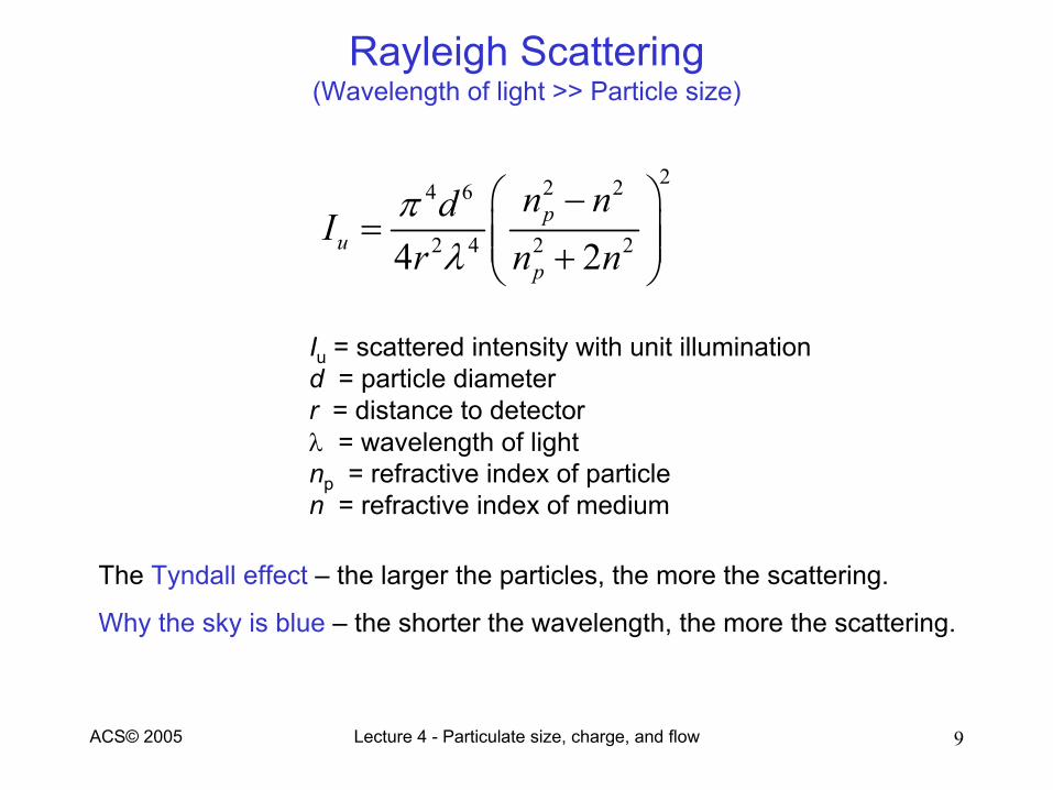
Rayleigh Scattering(Wavelength of light >> Particle size)
22 24 6
2 4 2 24 2p
up
n ndIr n nπ
λ −
= +
Iu = scattered intensity with unit illuminationd = particle diameterr = distance to detectorλ = wavelength of lightnp = refractive index of particlen = refractive index of medium
The Tyndall effect – the larger the particles, the more the scattering.
Why the sky is blue – the shorter the wavelength, the more the scattering.
Lecture 4 - Particulate size, charge, and flow 10ACS© 2005
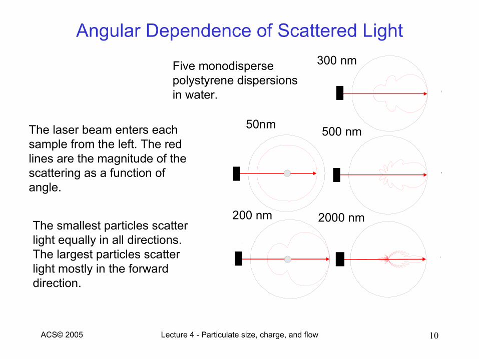
Angular Dependence of Scattered Light
1
p
p
1
p
p
1
p
p
1
p
p
1
p
p
50nm
200 nm
300 nm
500 nm
2000 nm
Five monodisperse polystyrene dispersions in water.
The laser beam enters each sample from the left. The red lines are the magnitude of the scattering as a function of angle.
The smallest particles scatter light equally in all directions.The largest particles scatter light mostly in the forward direction.
Lecture 4 - Particulate size, charge, and flow 11ACS© 2005
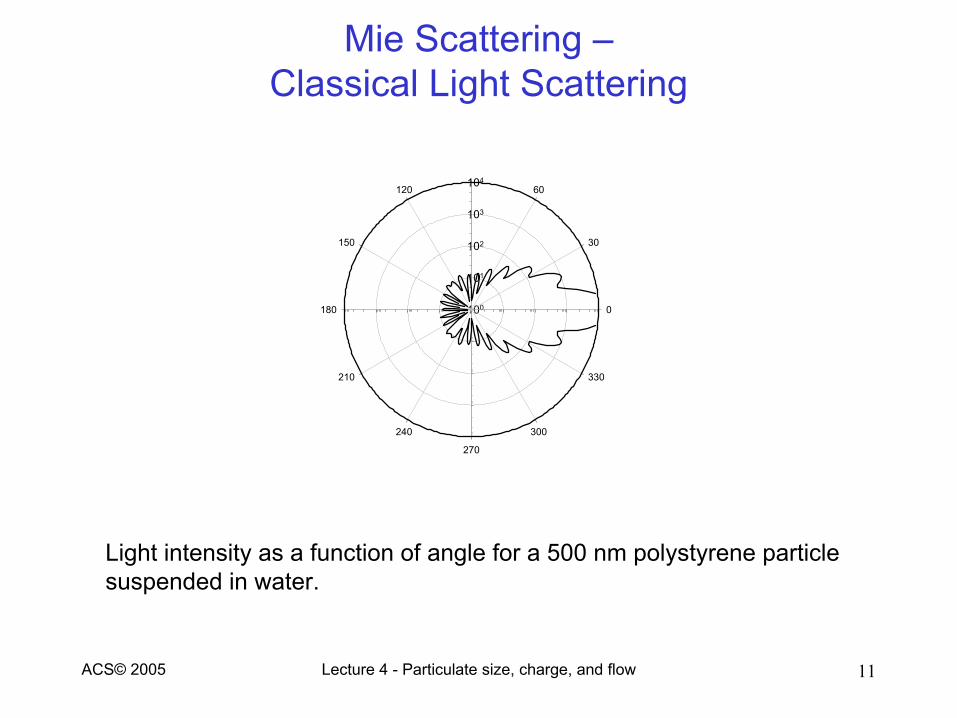
Mie Scattering –Classical Light Scattering
Light intensity as a function of angle for a 500 nm polystyrene particle suspended in water.
100
101
102
103
104
0
30
60120
150
180
210
240
270
300
330
Lecture 4 - Particulate size, charge, and flow 12ACS© 2005
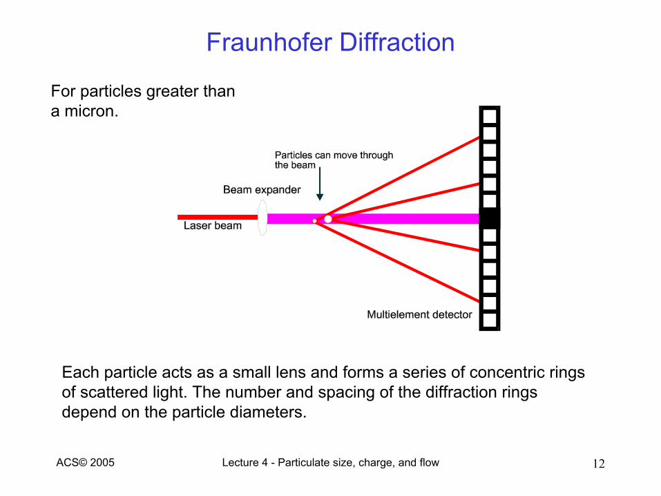
Fraunhofer Diffraction
For particles greater than a micron.
Each particle acts as a small lens and forms a series of concentric rings of scattered light. The number and spacing of the diffraction rings depend on the particle diameters.
Lecture 4 - Particulate size, charge, and flow 13ACS© 2005
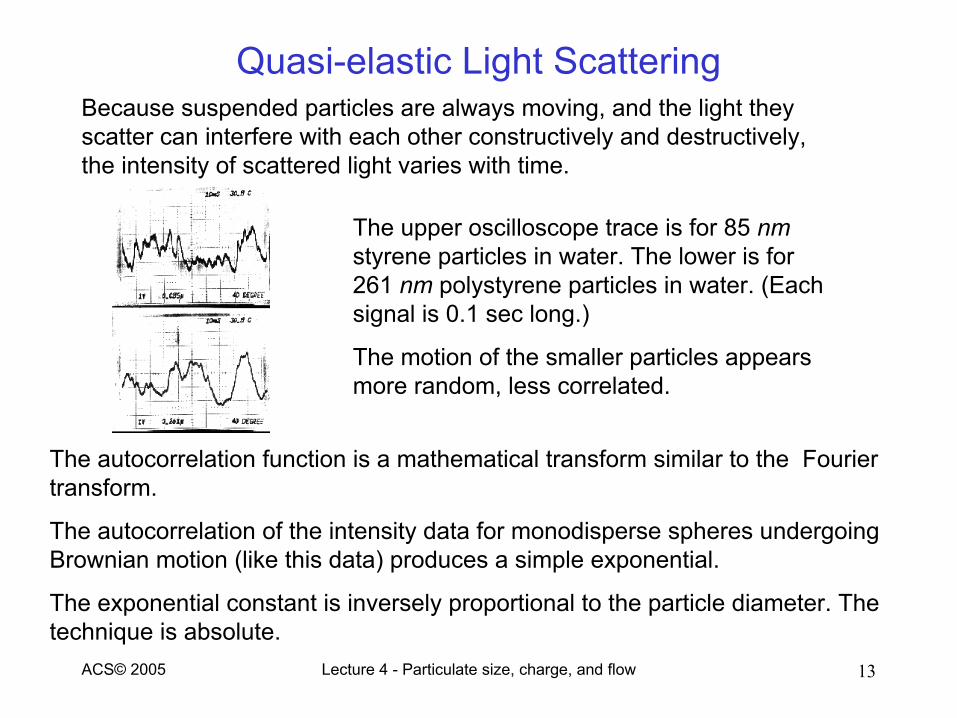
Quasi-elastic Light ScatteringBecause suspended particles are always moving, and the light they scatter can interfere with each other constructively and destructively, the intensity of scattered light varies with time.
The upper oscilloscope trace is for 85 nmstyrene particles in water. The lower is for 261 nm polystyrene particles in water. (Each signal is 0.1 sec long.)
The motion of the smaller particles appears more random, less correlated.
The autocorrelation function is a mathematical transform similar to the Fourier transform.
The autocorrelation of the intensity data for monodisperse spheres undergoing Brownian motion (like this data) produces a simple exponential.
The exponential constant is inversely proportional to the particle diameter. The technique is absolute.
Lecture 4 - Particulate size, charge, and flow 14ACS© 2005
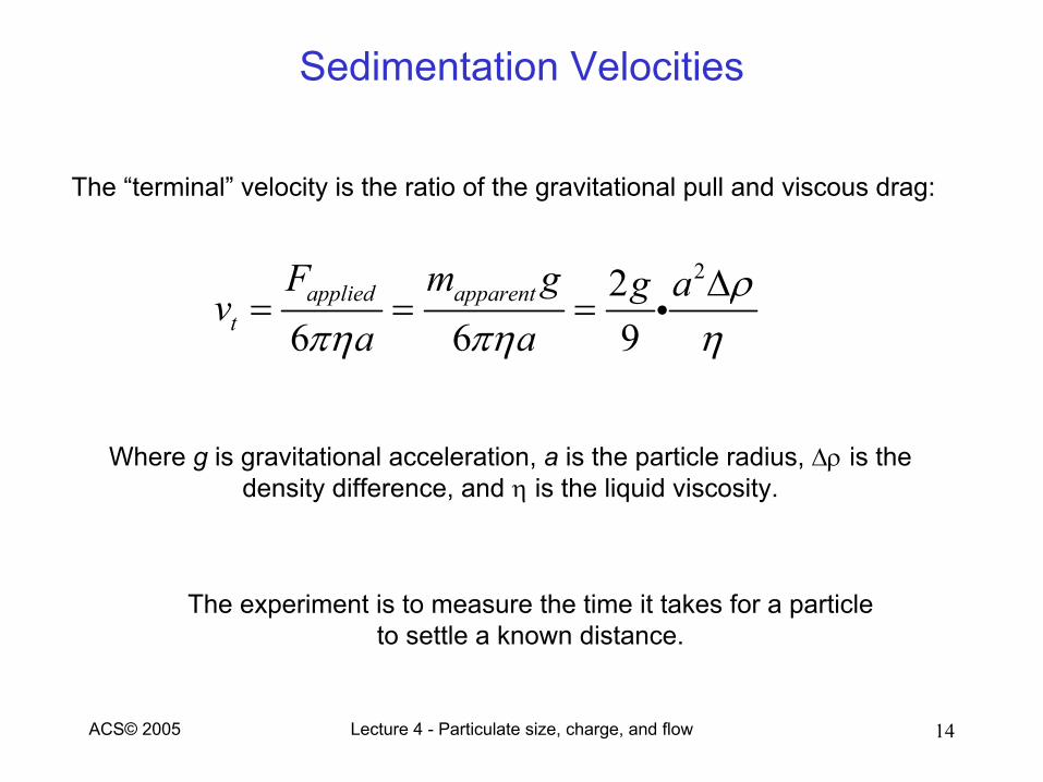
Sedimentation Velocities
226 6 9
ρπη πη η
∆= = = iapplied apparent
t
F m g g ava a
The “terminal” velocity is the ratio of the gravitational pull and viscous drag:
The experiment is to measure the time it takes for a particle to settle a known distance.
Where g is gravitational acceleration, a is the particle radius, ∆ρ is the density difference, and η is the liquid viscosity.
Lecture 4 - Particulate size, charge, and flow 15ACS© 2005
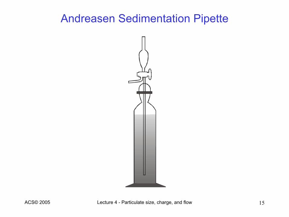
Andreasen Sedimentation Pipette
Lecture 4 - Particulate size, charge, and flow 16ACS© 2005
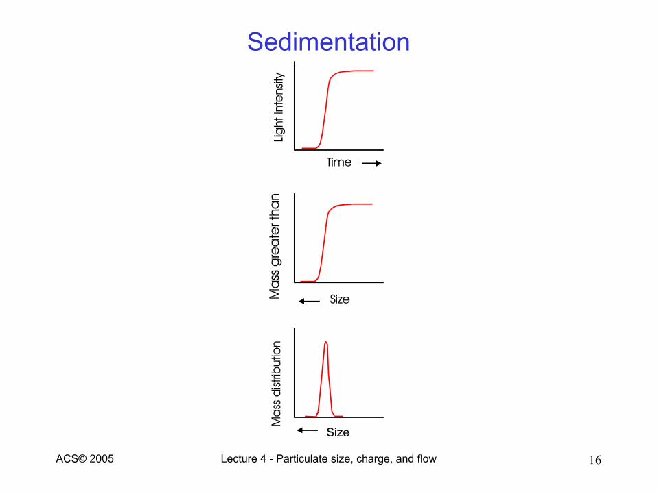
Sedimentation
Lecture 4 - Particulate size, charge, and flow 17ACS© 2005
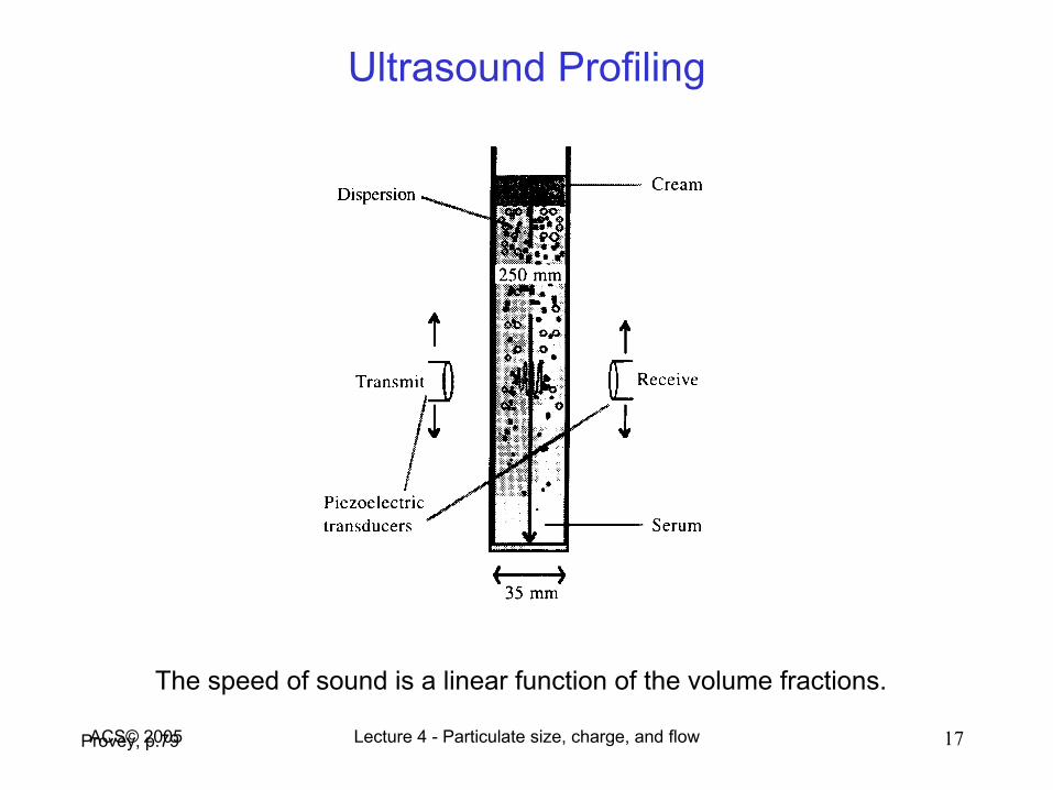
Ultrasound Profiling
Provey, p.79
The speed of sound is a linear function of the volume fractions.
Lecture 4 - Particulate size, charge, and flow 18ACS© 2005
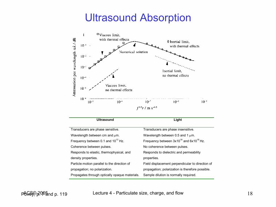
Ultrasound Absorption
Povey, p. 7 and p. 119
Ultrasound Light
Transducers are phase sensitive. Transducers are phase insensitive.
Wavelength between cm and µm. Wavelength between 0.5 and 1 µm.
Frequency between 0.1 and 1013 Hz. Frequency between 3x10¹⁶ and 6x10¹⁶ Hz.
Coherence between pulses. No coherence between pulses.
Responds to elastic, thermophysical, and
density properties.
Responds to dielectric and permeability
properties.
Particle motion parallel to the direction of
propagation; no polarization.
Field displacement perpendicular to direction of
propagation; polarization is therefore possible.
Propagates through optically opaque materials. Sample dilution is normally required.
Lecture 4 - Particulate size, charge, and flow 19ACS© 2005
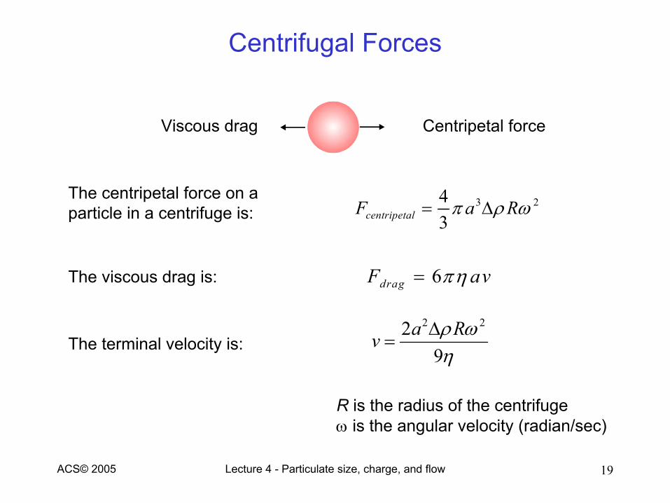
Centrifugal Forces
2 229
a Rv ρ ωη
∆=
The centripetal force on a particle in a centrifuge is:
3 243centripetalF a Rπ ρ ω= ∆
Centripetal forceViscous drag
The viscous drag is: 6dragF avπη=
The terminal velocity is:
R is the radius of the centrifugeω is the angular velocity (radian/sec)
Lecture 4 - Particulate size, charge, and flow 20ACS© 2005
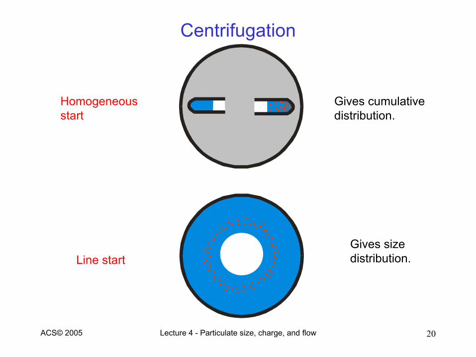
Centrifugation
Homogeneousstart
Line start
Gives cumulative distribution.
Gives size distribution.
Lecture 4 - Particulate size, charge, and flow 21ACS© 2005
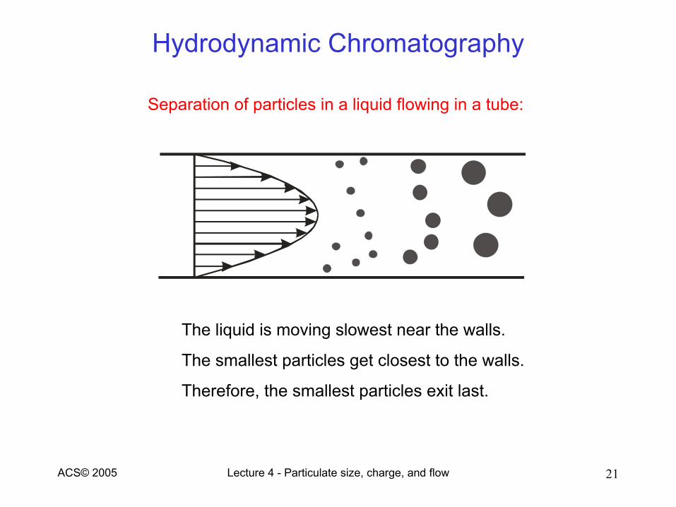
Hydrodynamic Chromatography
Separation of particles in a liquid flowing in a tube:
The liquid is moving slowest near the walls.
The smallest particles get closest to the walls.
Therefore, the smallest particles exit last.
Lecture 4 - Particulate size, charge, and flow 22ACS© 2005
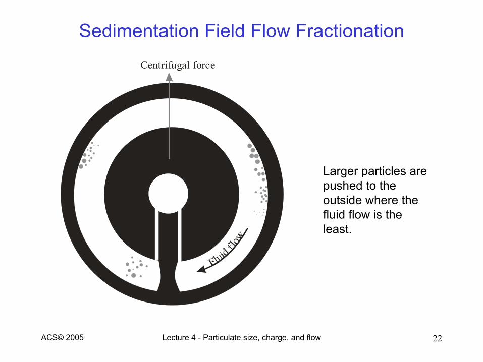
Sedimentation Field Flow Fractionation
Larger particles are pushed to the outside where the fluid flow is the least.
Centrifugal force
Lecture 4 - Particulate size, charge, and flow 23ACS© 2005
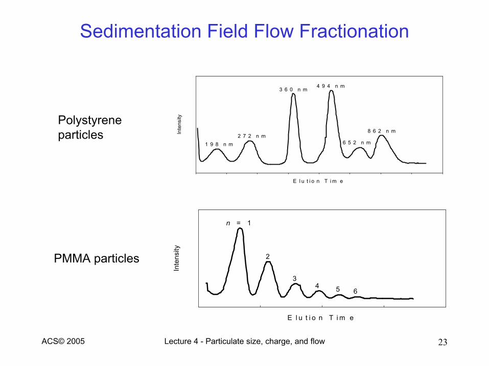
Sedimentation Field Flow Fractionation
E l u t i o n T i m eIn
tens
ity
1 9 8 n m2 7 2 n m
3 6 0 n m4 9 4 n m
6 5 2 n m
8 6 2 n m
E l u t i o n T i m e
Inte
nsity
n = 1
2
34 5 6
PMMA particles
Polystyrene particles
Lecture 4 - Particulate size, charge, and flow 24ACS© 2005
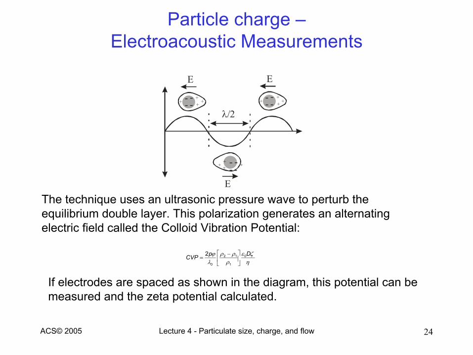
Particle charge –Electroacoustic Measurements
The technique uses an ultrasonic pressure wave to perturb the equilibrium double layer. This polarization generates an alternating electric field called the Colloid Vibration Potential:
02 1
0 1
2 DpCVP ε ζϕ ρ ρλ ρ η
−=
If electrodes are spaced as shown in the diagram, this potential can be measured and the zeta potential calculated.
-+++ +--
- -+++ +--
-
- +
+++ - -
-
E
EE
λ/2
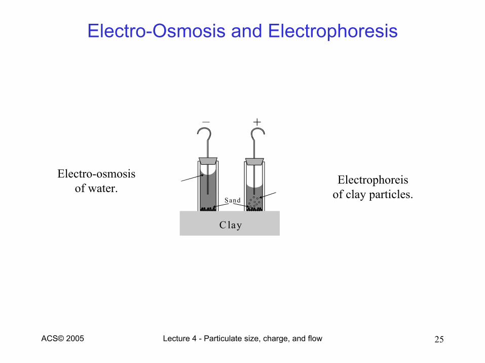
Lecture 4 - Particulate size, charge, and flow 25ACS© 2005
Electro-Osmosis and Electrophoresis
_ +
C lay
Sand
Electrophoreisof clay particles.
Electro-osmosisof water.
Lecture 4 - Particulate size, charge, and flow 26ACS© 2005
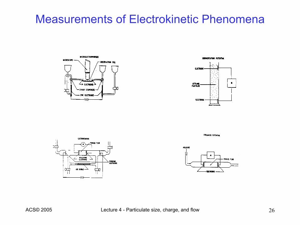
Measurements of Electrokinetic Phenomena
Lecture 4 - Particulate size, charge, and flow 27ACS© 2005
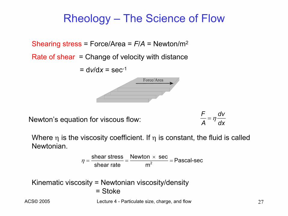
Rheology – The Science of Flow
Shearing stress = Force/Area = F/A = Newton/m2
Rate of shear = Change of velocity with distance
= dv/dx = sec-1
Newton’s equation for viscous flow:F dvA dx
η=
Where η is the viscosity coefficient. If η is constant, the fluid is called Newtonian.
η ×= = =2
shear stress Newton sec Pascal-secshear rate m
Kinematic viscosity = Newtonian viscosity/density= Stoke
Force/Area
Lecture 4 - Particulate size, charge, and flow 28ACS© 2005
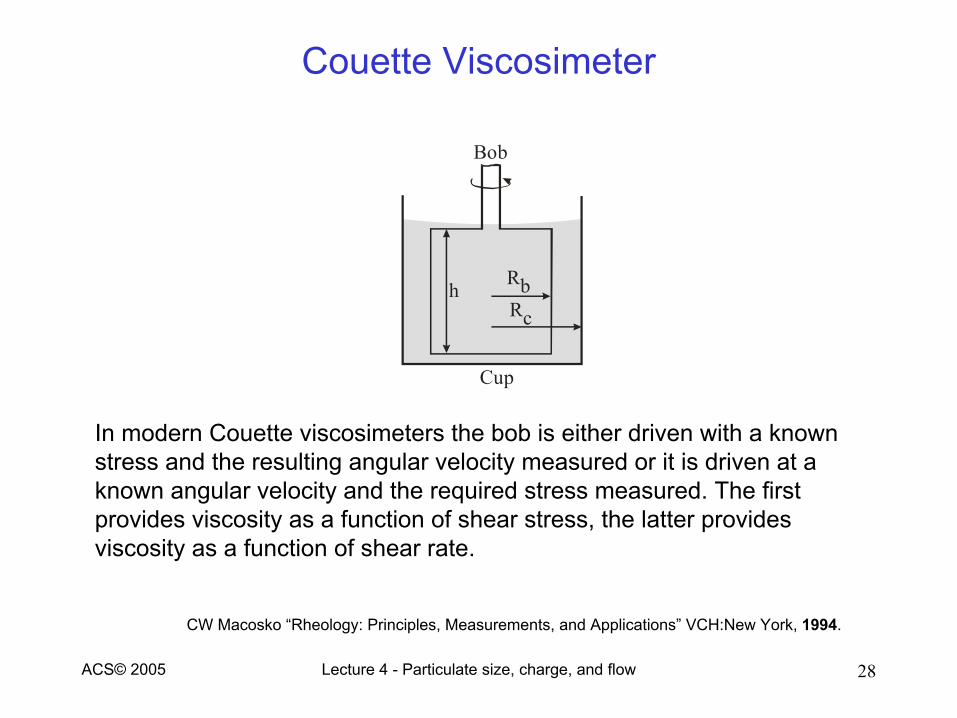
Couette Viscosimeter
In modern Couette viscosimeters the bob is either driven with a known stress and the resulting angular velocity measured or it is driven at a known angular velocity and the required stress measured. The first provides viscosity as a function of shear stress, the latter provides viscosity as a function of shear rate.
CW Macosko “Rheology: Principles, Measurements, and Applications” VCH:New York, 1994.
Bob
Cup
RbRc
h
Lecture 4 - Particulate size, charge, and flow 29ACS© 2005
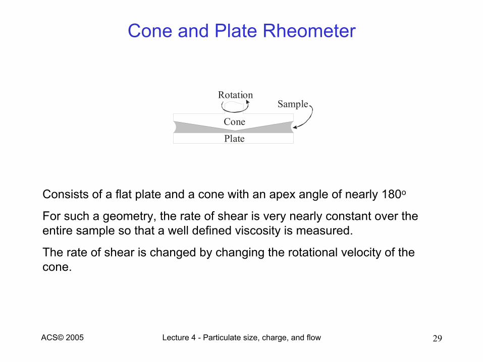
Cone and Plate Rheometer
Consists of a flat plate and a cone with an apex angle of nearly 180o
For such a geometry, the rate of shear is very nearly constant over the entire sample so that a well defined viscosity is measured.
The rate of shear is changed by changing the rotational velocity of the cone.
Cone
Plate
SampleRotation
Lecture 4 - Particulate size, charge, and flow 30ACS© 2005
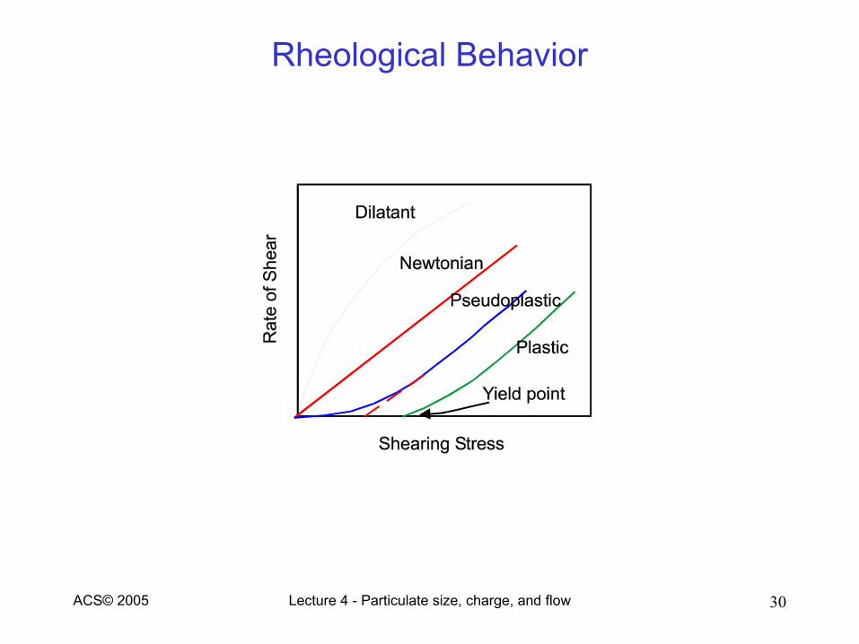
Rheological Behavior
Lecture 4 - Particulate size, charge, and flow 31ACS© 2005
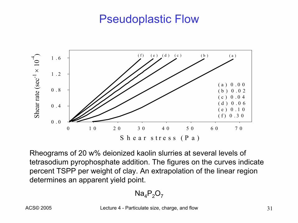
Pseudoplastic Flow
Rheograms of 20 w% deionized kaolin slurries at several levels of tetrasodium pyrophosphate addition. The figures on the curves indicate percent TSPP per weight of clay. An extrapolation of the linear region determines an apparent yield point.
Na4P2O7
S h e a r s t r e s s ( P a )0 1 0 2 0 3 0 4 0 5 0 6 0 7 0
Shea
r rat
e (s
ec-1
× 1
0-4)
0 . 0
0 . 4
0 . 8
1 . 2
1 . 6
( a ) 0 . 0 0( b ) 0 . 0 2( c ) 0 . 0 4( d ) 0 . 0 6( e ) 0 . 1 0( f ) 0 . 3 0
( a )( b )( c )( d )( e )( f )
Lecture 4 - Particulate size, charge, and flow 32ACS© 2005
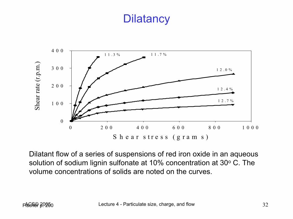
Dilatancy
Fischer p. 200
Dilatant flow of a series of suspensions of red iron oxide in an aqueous solution of sodium lignin sulfonate at 10% concentration at 30o C. The volume concentrations of solids are noted on the curves.
S h e a r s t r e s s ( g r a m s )0 2 0 0 4 0 0 6 0 0 8 0 0 1 0 0 0
Shea
r rat
e (r
.p.m
.)
0
1 0 0
2 0 0
3 0 0
4 0 01 1 . 3 % 1 1 . 7 %
1 2 . 0 %
1 2 . 4 %
1 2 . 7 %
Lecture 4 - Particulate size, charge, and flow 33ACS© 2005
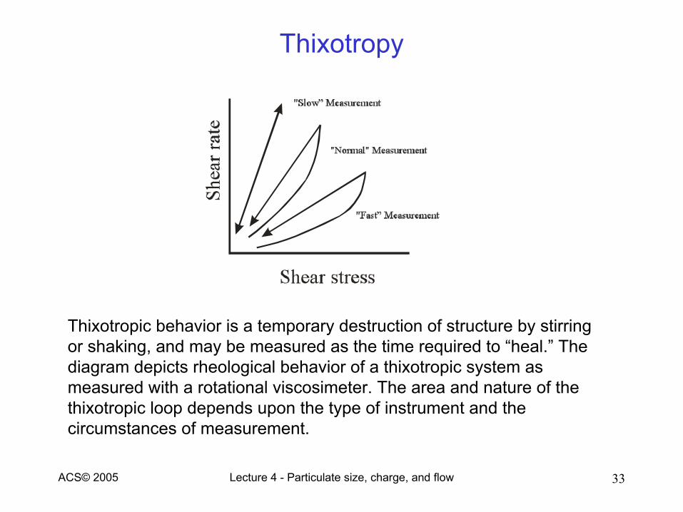
Thixotropy
Thixotropic behavior is a temporary destruction of structure by stirring or shaking, and may be measured as the time required to “heal.” The diagram depicts rheological behavior of a thixotropic system as measured with a rotational viscosimeter. The area and nature of the thixotropic loop depends upon the type of instrument and the circumstances of measurement.