Specification of the Bayesian CRM: Model and Sample Size

Ken Cheung Department of Biostatistics, Columbia University

Ken Cheung 2

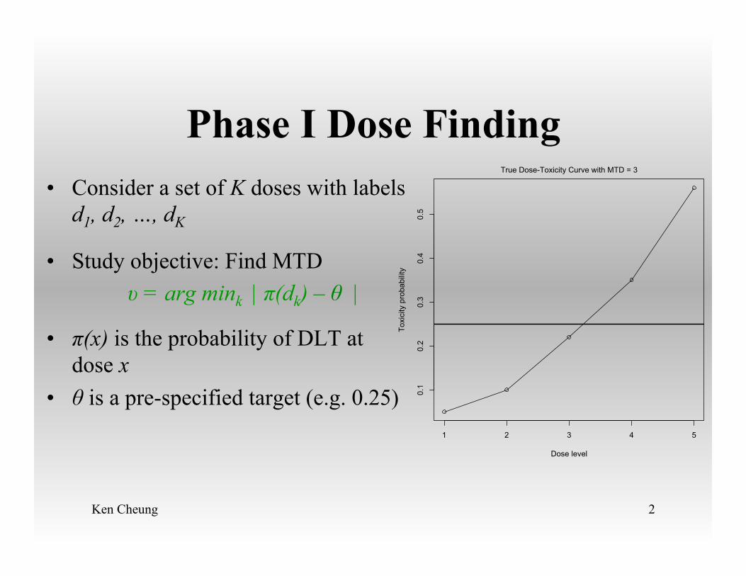
Phase I Dose Finding •  Consider a set of K doses with labels

d1, d2, …, dK

•  Study objective: Find MTD υ = arg mink

| π(dk) – θ |

•  π(x) is the probability of DLT at dose x

•  θ is a pre-specified target (e.g. 0.25) 1 2 3 4 5

0.1

0.2

0.3

0.4

0.5

Dose level

Toxi

city

pro

babi

lity

True Dose-Toxicity Curve with MTD = 3

CRM

•  First proposed by O’Quigley et al. (1990) •  Model-based •  Single-parameter model •  Bayesian-flavor •  “Myopic” •  Many variations and extensions

•  Two-parameter or curve free; MLE; Continuous dosage; EWOC

Ken Cheung 3

CRM

•  This talk focuses specifically on the original version of the Bayesian CRM (1990).

•  Treat patients sequentially at dose level υn = arg mink

| F(dk , bn ) – θ | •  The dose-toxicity function F(x, β) is one-parameter, with a

prior distribution on β.

•  bn is the posterior mean of β

•  Patient 1 gets prior MTD

•  Recall study objective – MTD υ = arg mink | π(dk) – θ |

Ken Cheung 4

CRM

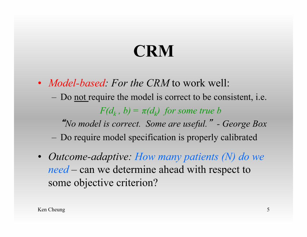
•  Model-based: For the CRM to work well: –  Do not require the model is correct to be consistent, i.e.

F(dk , b) = π(dk) for some true b “No model is correct. Some are useful.” - George Box

–  Do require model specification is properly calibrated

•  Outcome-adaptive: How many patients (N) do we need – can we determine ahead with respect to some objective criterion?

Ken Cheung 5

Objectives of this talk

•  Present an approach to specify the Bayesian CRM model in a timely and reproducible manner

•  Present a sample size formula for the CRM model obtained via the specification process

•  Provide practical guidelines on using the sample size formula

Ken Cheung 6

Ken Cheung 7

Outline of this talk

•  Calibration of a Bayesian CRM model – Dose-toxicity function –  Initial guesses of DLT rates (“Skeleton”) – Prior distribution of model parameter

•  Sample size formulae for a properly calibrated CRM

•  Example: A PTEN-long trial

Ken Cheung 8

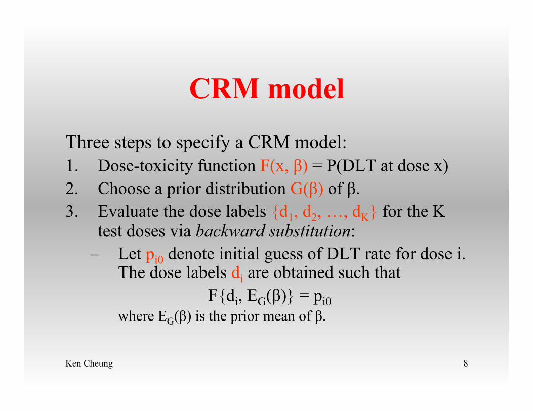
CRM model

Three steps to specify a CRM model: 1.  Dose-toxicity function F(x, β) = P(DLT at dose x) 2.  Choose a prior distribution G(β) of β. 3.  Evaluate the dose labels {d1, d2, …, dK} for the K

test doses via backward substitution: –  Let pi0 denote initial guess of DLT rate for dose i.

The dose labels di are obtained such that F{di, EG(β)} = pi0

where EG(β) is the prior mean of β.

Ken Cheung 9

CRM model

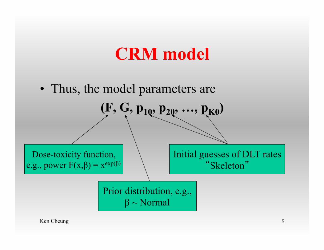
•  Thus, the model parameters are (F, G, p10, p20, …, pK0)

Dose-toxicity function,

e.g., power F(x,β) = xexp(β)

Prior distribution, e.g., β ~ Normal

Initial guesses of DLT rates “Skeleton”

Ken Cheung 10

CRM model

•  Lee and Cheung (2009): For any fixed F and G, we can choose the skeleton {p10, p20, …, pK0 }to match the operating characteristics

•  Approach: Reduce the specification problem of K numbers to 2 meaningful inputs –  The prior MTD, υ0 = Starting dose level –  An acceptable range of toxicity rate θ ± δ, where θ is

the target toxicity rate. E.g., 0.25 ± 0.05

Ken Cheung 11

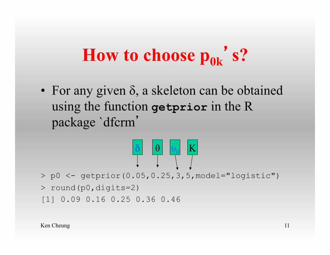
How to choose p0k’s?

•  For any given δ, a skeleton can be obtained using the function getprior in the R package `dfcrm’

> p0 <- getprior(0.05,0.25,3,5,model="logistic")

> round(p0,digits=2) [1] 0.09 0.16 0.25 0.36 0.46

δ θ υ0 K

Ken Cheung 12

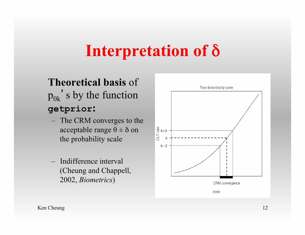
Interpretation of δ

Theoretical basis of p0k’s by the function getprior: –  The CRM converges to the

acceptable range θ ± δ on the probability scale

–  Indifference interval (Cheung and Chappell, 2002, Biometrics)

Ken Cheung 13

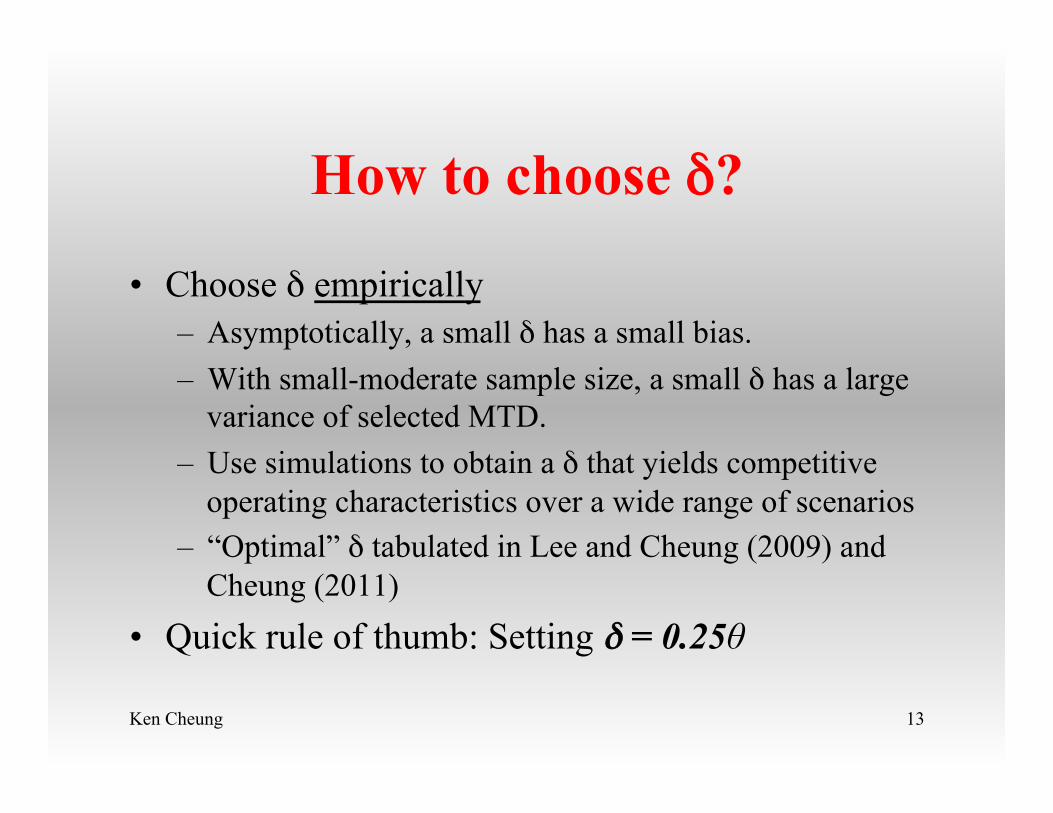
How to choose δ?

•  Choose δ empirically –  Asymptotically, a small δ has a small bias. –  With small-moderate sample size, a small δ has a large

variance of selected MTD. –  Use simulations to obtain a δ that yields competitive

operating characteristics over a wide range of scenarios –  “Optimal” δ tabulated in Lee and Cheung (2009) and

Cheung (2011)

•  Quick rule of thumb: Setting δ = 0.25θ

Ken Cheung 14

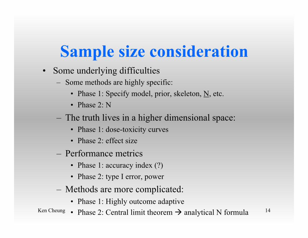
Sample size consideration •  Some underlying difficulties

–  Some methods are highly specific: •  Phase 1: Specify model, prior, skeleton, N, etc. •  Phase 2: N

–  The truth lives in a higher dimensional space: •  Phase 1: dose-toxicity curves •  Phase 2: effect size

–  Performance metrics •  Phase 1: accuracy index (?) •  Phase 2: type I error, power

–  Methods are more complicated: •  Phase 1: Highly outcome adaptive •  Phase 2: Central limit theorem à analytical N formula

Ken Cheung 15

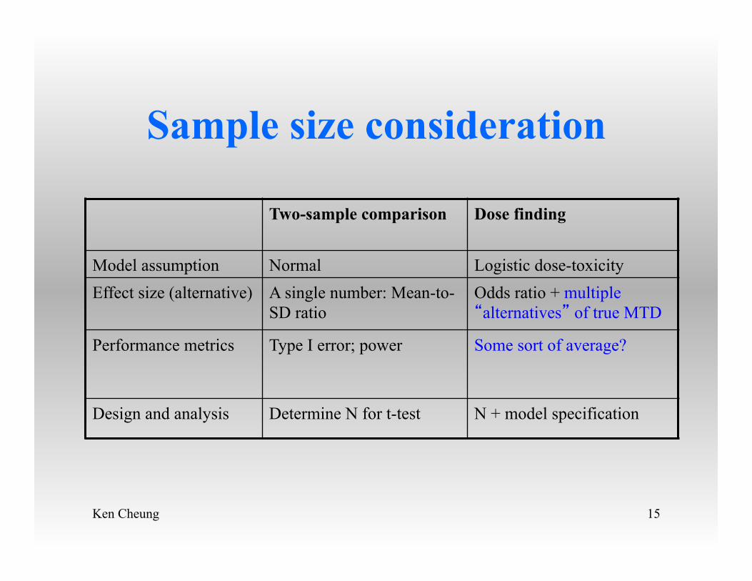
Sample size consideration

Two-sample comparison Dose finding

Model assumption Normal Logistic dose-toxicity Effect size (alternative) A single number: Mean-to-

SD ratio Odds ratio + multiple “alternatives” of true MTD

Performance metrics Type I error; power Some sort of average?

Design and analysis Determine N for t-test N + model specification

Ken Cheung 16

Sample size consideration

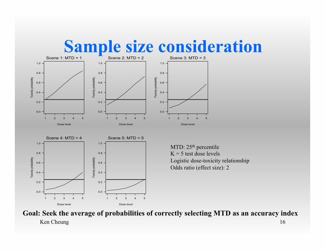
MTD: 25th percentile K = 5 test dose levels Logistic dose-toxicity relationship Odds ratio (effect size): 2

Goal: Seek the average of probabilities of correctly selecting MTD as an accuracy index

1 2 3 4 5

0.0

0.2

0.4

0.6

0.8

1.0

Dose level

Toxic

ity p

roba

bility

Scene 1: MTD = 1

1 2 3 4 5

0.0

0.2

0.4

0.6

0.8

1.0

Dose level

Toxic

ity p

roba

bility

Scene 2: MTD = 2

1 2 3 4 5

0.0

0.2

0.4

0.6

0.8

1.0

Dose level

Toxic

ity p

roba

bility

Scene 3: MTD = 3

1 2 3 4 5

0.0

0.2

0.4

0.6

0.8

1.0

Dose level

Toxic

ity p

roba

bility

Scene 4: MTD = 4

1 2 3 4 5

0.0

0.2

0.4

0.6

0.8

1.0

Dose level

Toxic

ity p

roba

bility

Scene 5: MTD = 5

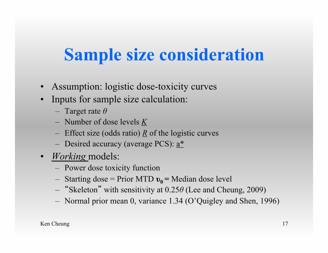
Sample size consideration •  Assumption: logistic dose-toxicity curves •  Inputs for sample size calculation:

–  Target rate θ –  Number of dose levels K –  Effect size (odds ratio) R of the logistic curves –  Desired accuracy (average PCS): a*

•  Working models: –  Power dose toxicity function –  Starting dose = Prior MTD υ0 = Median dose level –  “Skeleton” with sensitivity at 0.25θ (Lee and Cheung, 2009) –  Normal prior mean 0, variance 1.34 (O’Quigley and Shen, 1996)

Ken Cheung 17

Ken Cheung 18

Sample size consideration

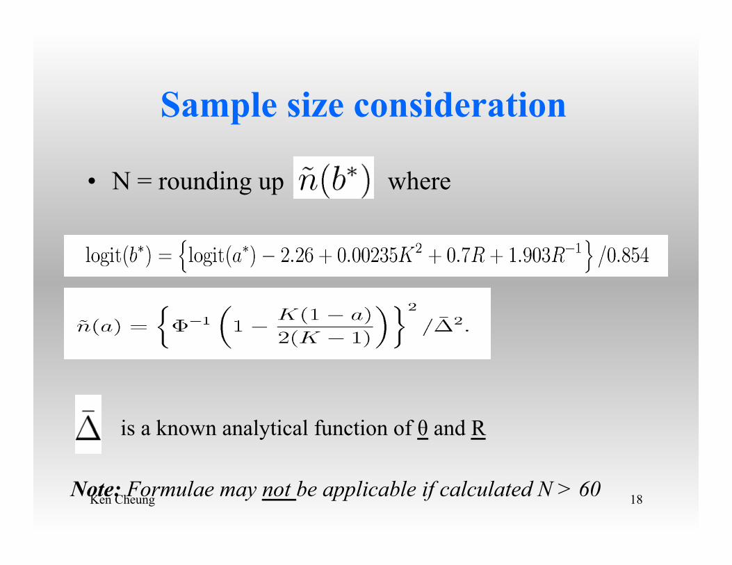
•  N = rounding up where

is a known analytical function of θ and R

Note: Formulae may not be applicable if calculated N > 60

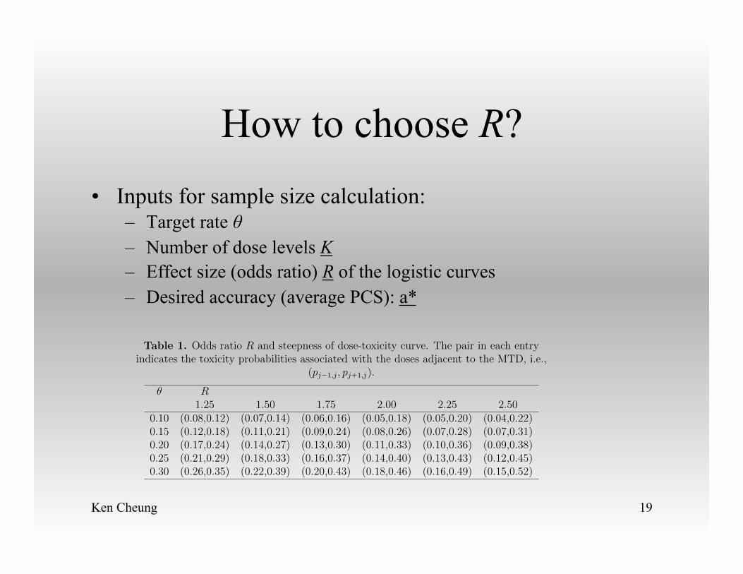
How to choose R? •  Inputs for sample size calculation:

–  Target rate θ –  Number of dose levels K –  Effect size (odds ratio) R of the logistic curves –  Desired accuracy (average PCS): a*

Ken Cheung 19

Table 1. Odds ratio R and steepness of dose-toxicity curve. The pair in each entryindicates the toxicity probabilities associated with the doses adjacent to the MTD, i.e.,

(pj�1,j, pj+1,j).

✓ R1.25 1.50 1.75 2.00 2.25 2.50

0.10 (0.08,0.12) (0.07,0.14) (0.06,0.16) (0.05,0.18) (0.05,0.20) (0.04,0.22)0.15 (0.12,0.18) (0.11,0.21) (0.09,0.24) (0.08,0.26) (0.07,0.28) (0.07,0.31)0.20 (0.17,0.24) (0.14,0.27) (0.13,0.30) (0.11,0.33) (0.10,0.36) (0.09,0.38)0.25 (0.21,0.29) (0.18,0.33) (0.16,0.37) (0.14,0.40) (0.13,0.43) (0.12,0.45)0.30 (0.26,0.35) (0.22,0.39) (0.20,0.43) (0.18,0.46) (0.16,0.49) (0.15,0.52)

19

Ken Cheung 20

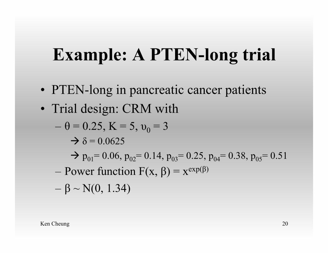
Example: A PTEN-long trial

•  PTEN-long in pancreatic cancer patients •  Trial design: CRM with

–  θ = 0.25, K = 5, υ0 = 3 à  δ = 0.0625 à  p01= 0.06, p02= 0.14, p03= 0.25, p04= 0.38, p05= 0.51

– Power function F(x, β) = xexp(β) –  β ~ N(0, 1.34)

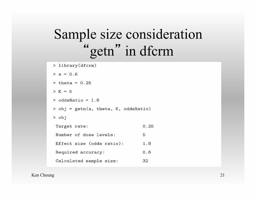
Sample size consideration “getn” in dfcrm

Ken Cheung 21

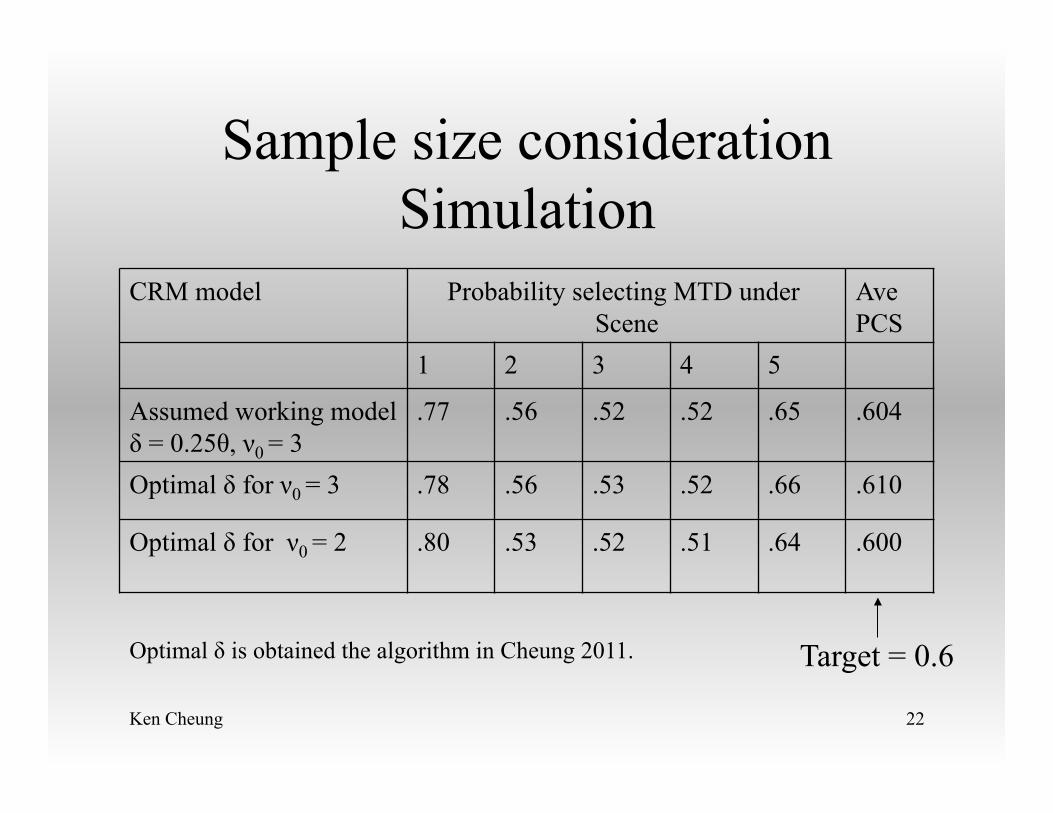
Sample size consideration Simulation

Ken Cheung 22

CRM model Probability selecting MTD under Scene

Ave PCS

1 2 3 4 5

Assumed working model δ = 0.25θ, ν0 = 3

.77 .56 .52 .52 .65 .604

Optimal δ for ν0 = 3 .78 .56 .53 .52 .66 .610

Optimal δ for ν0 = 2 .80 .53 .52 .51 .64 .600

Target = 0.6 Optimal δ is obtained the algorithm in Cheung 2011.

Ken Cheung 23

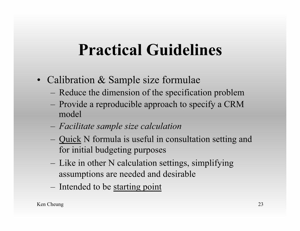
Practical Guidelines

•  Calibration & Sample size formulae –  Reduce the dimension of the specification problem –  Provide a reproducible approach to specify a CRM

model –  Facilitate sample size calculation –  Quick N formula is useful in consultation setting and

for initial budgeting purposes –  Like in other N calculation settings, simplifying

assumptions are needed and desirable –  Intended to be starting point

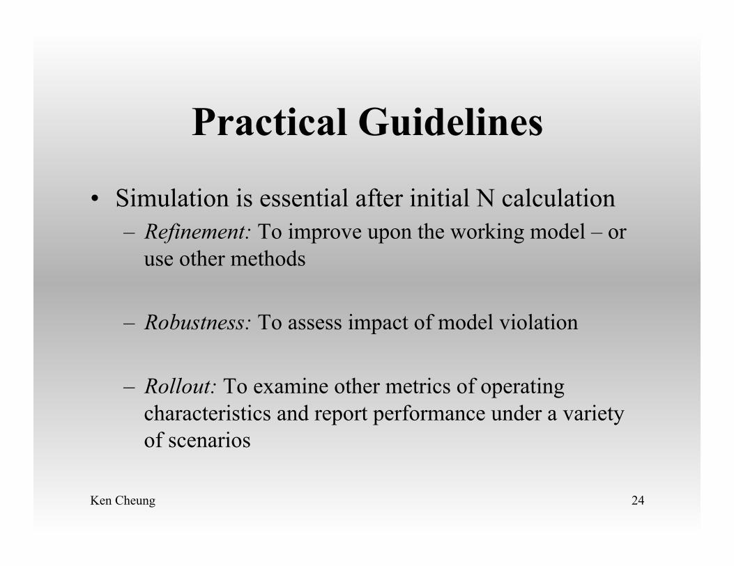
Practical Guidelines

•  Simulation is essential after initial N calculation –  Refinement: To improve upon the working model – or

use other methods

–  Robustness: To assess impact of model violation

–  Rollout: To examine other metrics of operating characteristics and report performance under a variety of scenarios

Ken Cheung 24

Useful Resources

•  “dfcrm” library in R –  Version 0.2-2 [update if you have 0.2-1]

•  Main references –  Lee and Cheung (2009): Model calibration in the CRM.

Clinical Trials 6:227—238. –  Cheung (2011). Dose Finding by the Continual

Reassessment Method. CRC Press/Taylor & Francis Group

–  Cheung (2013): Sample size formulae for the Bayesian CRM. Clinical Trials in press.

Ken Cheung 25