Part A Electromagnetism - University of Oxfordusers.ox.ac.uk/~math0391/EMlectures.pdf · 0.3...
38
Part A Electromagnetism James Sparks [email protected] Hilary Term 2009 ∇· E = ρ ǫ 0 ∇· B =0 ∇∧ E = − ∂ B ∂t ∇∧ B = μ 0 J + ǫ 0 ∂ E ∂t
Transcript of Part A Electromagnetism - University of Oxfordusers.ox.ac.uk/~math0391/EMlectures.pdf · 0.3...
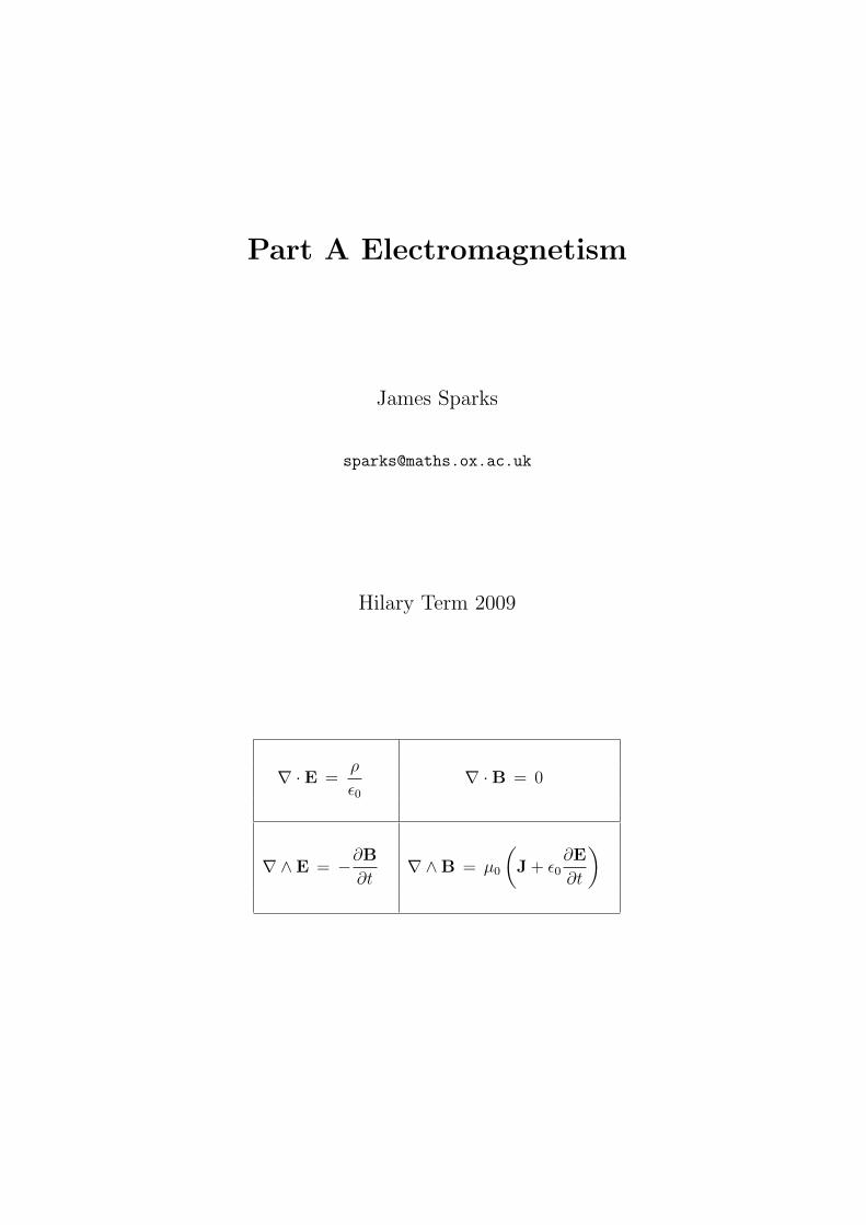
Part A Electromagnetism
James Sparks
Hilary Term 2009
∇ · E =ρ
ǫ0
∇ · B = 0
∇∧ E = −∂B
∂t∇∧ B = µ0
(J + ǫ0
∂E
∂t
)
Contents
0 Introduction ii
0.1 About these notes . . . . . . . . . . . . . . . . . . . . . . . . . . . . . . . . . ii
0.2 Preamble . . . . . . . . . . . . . . . . . . . . . . . . . . . . . . . . . . . . . . ii
0.3 Bibliography . . . . . . . . . . . . . . . . . . . . . . . . . . . . . . . . . . . . iii
0.4 Preliminary comments . . . . . . . . . . . . . . . . . . . . . . . . . . . . . . . iii
1 Electrostatics 1
1.1 Point charges and Coulomb’s law . . . . . . . . . . . . . . . . . . . . . . . . . 1
1.2 The electric field . . . . . . . . . . . . . . . . . . . . . . . . . . . . . . . . . . 2
1.3 Gauss’ law . . . . . . . . . . . . . . . . . . . . . . . . . . . . . . . . . . . . . . 2
1.4 Charge density and Gauss’ law . . . . . . . . . . . . . . . . . . . . . . . . . . 4
1.5 The electrostatic potential and Poisson’s equation . . . . . . . . . . . . . . . 5
1.6 Boundary conditions and surface charge . . . . . . . . . . . . . . . . . . . . . 7
1.7 Electrostatic energy . . . . . . . . . . . . . . . . . . . . . . . . . . . . . . . . 9
2 Magnetostatics 11
2.1 Electric currents . . . . . . . . . . . . . . . . . . . . . . . . . . . . . . . . . . 11
2.2 The continuity equation . . . . . . . . . . . . . . . . . . . . . . . . . . . . . . 12
2.3 The Lorentz force and the magnetic field . . . . . . . . . . . . . . . . . . . . . 12
2.4 The Biot-Savart law . . . . . . . . . . . . . . . . . . . . . . . . . . . . . . . . 13
2.5 Magnetic monopoles? . . . . . . . . . . . . . . . . . . . . . . . . . . . . . . . 15
2.6 Ampere’s law . . . . . . . . . . . . . . . . . . . . . . . . . . . . . . . . . . . . 16
2.7 The magnetostatic vector potential . . . . . . . . . . . . . . . . . . . . . . . . 18
3 Electrodynamics and Maxwell’s equations 19
3.1 Maxwell’s displacement current . . . . . . . . . . . . . . . . . . . . . . . . . . 19
3.2 Faraday’s law . . . . . . . . . . . . . . . . . . . . . . . . . . . . . . . . . . . . 20
3.3 Maxwell’s equations . . . . . . . . . . . . . . . . . . . . . . . . . . . . . . . . 21
3.4 Electromagnetic potentials and gauge invariance . . . . . . . . . . . . . . . . 22
3.5 Electromagnetic energy and Poynting’s theorem . . . . . . . . . . . . . . . . . 23
4 Electromagnetic waves 24
4.1 Source-free equations and electromagnetic waves . . . . . . . . . . . . . . . . 24
4.2 Monochromatic plane waves . . . . . . . . . . . . . . . . . . . . . . . . . . . . 25
4.3 Polarization . . . . . . . . . . . . . . . . . . . . . . . . . . . . . . . . . . . . . 26
i
4.4 Reflection . . . . . . . . . . . . . . . . . . . . . . . . . . . . . . . . . . . . . . 28
A Summary: vector calculus I
A.1 Vectors in R3 . . . . . . . . . . . . . . . . . . . . . . . . . . . . . . . . . . . . I
A.2 Vector operators . . . . . . . . . . . . . . . . . . . . . . . . . . . . . . . . . . I
A.3 Integral theorems . . . . . . . . . . . . . . . . . . . . . . . . . . . . . . . . . . II
0 Introduction
0.1 About these notes
This is a working set of lecture notes for the Part A Electromagnetism course, which is part
of the mathematics syllabus at the University of Oxford. I have attempted to put together
a concise set of notes that describes the basics of electromagnetic theory to an audience
of undergraduate mathematicians. In particular, therefore, many of the important physical
applications are not covered. I claim no great originality for the content: for example, section
4.2 closely follows the treatment and notation in Woodhouse’s book (see section 0.3), while
section 4.4 is based on lecture notes of Prof Paul Tod.
Please send any questions/corrections/comments to [email protected].
0.2 Preamble
In this course we take a first look at the classical theory of electromagnetism. Historically,
this begins with Coulomb’s inverse square law force between stationary point charges, dating
from 1785, and culminates (for us, at least) with Maxwell’s formulation of electromagnetism
in his 1864 paper, A Dynamical Theory of the Electromagnetic Field. It was in the latter pa-
per that the electromagnetic wave equation was first written down, and in which Maxwell first
proposed that “light is an electromagnetic disturbance propagated through the field according
to electromagnetic laws”. Maxwell’s equations, which appear on the front of these lecture
notes, describe an astonishing number of physical phenomena, over an absolutely enormous
range of scales. For example, the electromagnetic force1 holds the negatively charged elec-
trons in orbit around the positively charged nucleus of an atom. Interactions between atoms
and molecules are also electromagnetic, so that chemical forces are really electromagnetic
forces. The electromagnetic force is essentially responsible for almost all physical phenom-
ena encountered in day-to-day experience, with the exception of gravity: friction, electricity,
electric motors, permanent magnets, electromagnets, lightning, electromagnetic radiation
(radiowaves, microwaves, X-rays, etc, as well as visible light), . . . it’s all electromagnetism.
1Quantum mechanics also plays an important role here, which I’m suppressing.
ii
0.3 Bibliography
This is a short, introductory course on electromagnetism, focusing more on the mathematical
formalism than on physical applications. Those who wish (and have time!) to learn more
about the physics are particularly encouraged to dip into some of the references below, which
are in no particular order:
• W. J. Duffin, Electricity and Magnetism, McGraw-Hill, fourth edition (2001), chapters
1-4, 7, 8, 13.
• N. M. J. Woodhouse, Special Relativity, Springer Undergraduate Mathematics, Springer
Verlag (2002), chapters 2, 3.
• R. P. Feynman, R. B. Leighton, M. Sands, The Feynman Lectures on Physics, Volume
2: Electromagnetism, Addison-Wesley.
• B. I. Bleaney, B. Bleaney, Electricity and Magnetism, OUP, third edition, chapters
1.1-4, 2 (except 2.3), 3.1-2, 4.1-2, 4.4, 5.1, 8.1-4.
• J. D. Jackson, Classical Electrodynamics, John Wiley, third edition (1998), chapters 1,
2, 5, 6, 7 (this is more advanced).
0.4 Preliminary comments
As described in the course synopsis, classical electromagnetism is an application of the three-
dimensional vector calculus you learned in Moderations: div, grad, curl, and the Stokes and
divergence theorems. Since this is only an 8 lecture course, I won’t have time to revise
this before we begin. However, I’ve included a brief appendix which summarizes the main
definitions and results. Please, please, please take a look at this after the first lecture, and
make sure you’re happy with everything there.
We’ll take a usual, fairly historical, route, by starting with Coulomb’s law in electrostatics,
and eventually building up to Maxwell’s equations on the front page. The disadvantage with
this is that you’ll begin by learning special cases of Maxwell’s equations – having learned
one equation, you will later find that more generally there are other terms in it. On the
other hand, simply starting with Maxwell’s equations and then deriving everything else from
them is probably too abstract, and doesn’t really give a feel for where the equations have
come from. My advice is that at the end of each lecture you should take another look at
the equations on the front cover – each time you should find that you understand better
what they mean. Starred paragraphs are not examinable, either because they are slightly
off-syllabus, or because they are more difficult.
There are 2 problem sheets for the course, for which solution sets are available.
iii
1 Electrostatics
1.1 Point charges and Coulomb’s law
It is a fact of nature that elementary particles have a property called electric charge. In SI
units2 this is measured in Coulombs C, and the electron and proton carry equal and opposite
charges ∓q, where q = 1.6022 × 10⁻¹⁹ C. Atoms consist of electrons orbiting a nucleus of
protons and neutrons (with the latter carrying charge 0), and thus all charges in stable matter,
made of atoms, arise from these electron and proton charges.
Electrostatics is the study of charges at rest. We model space by R3, or a subset thereof,
and represent the position of a stationary point charge q by the position vector r ∈ R3.
Given two such charges, q1, q2 at positions r1, r2, respectively, the first charge experiences3
an electrical force F1 due to the second charge given by
F1 =1
4πǫ0
q1q2
|r1 − r2|3(r1 − r2) . (1.1)
Note this only makes sense if r1 6= r2, which we thus assume. The constant ǫ0 is called the
permittivity of free space, which in SI units takes the value ǫ0 = 8.8542 × 10⁻¹² C2 N−1 m−2.
Without loss of generality, we might as well put the second charge at the origin r2 = 0,
denote r1 = r, q2 = q, and equivalently rewrite (1.1) as
F1 =1
4πǫ0
q1q
r2r (1.2)
where r = r/r is a unit vector and r = |r|. This is Coulomb’s law of electrostatics, and is an
experimental fact. Note that:
E1 : The force is proportional to the product of the charges, so that opposite
(different sign) charges attract, while like (same sign) charges repel.
E2 : The force acts in the direction of the vector joining the two charges, and
is inversely proportional to the square of the distance of separation.
The above two statements are equivalent to Coulomb’s law.
The final law of electrostatics says what happens when there are more than just two
charges:
E3 : Electrostatic forces obey the Principle of Superposition.
2where, for example, distance is measured in metres, time is measured in seconds, force is measured inNewtons.
3Of course, if this is the only force acting on the first charge, by Newton’s second law of motion it willnecessarily begin to move, and we are no longer dealing with statics.
1
That is, if we have N charges qi at positions ri, i = 1, . . . , N , then an additional charge q at
position r experiences a force
F =N∑
i=1
1
4πǫ0
qqi
|r − ri|3(r − ri) . (1.3)
So, to get the total force on charge q due to all the other charges, we simply add up (superpose)
the Coulomb force (1.1) from each charge qi.
1.2 The electric field
The following definition looks completely trivial at first sight, but in fact it’s an ingenious
shift of viewpoint. Given a particular distribution of charges, as above, we define the electric
field E = E(r) to be the force on a unit test charge (i.e. q = 1) at position r. Here the
nomenclature “test charge” indicates that the charge is not regarded as part of the distribution
of charges that it is “probing”. The force in (1.3) is thus
F = q E (1.4)
where by definition
E(r) =1
4πǫ0
N∑
i=1
qi
|r − ri|3(r − ri) (1.5)
is the electric field produced by the N charges. It is a vector field4, depending on position r.
As we have defined it, the electric field is just a mathematically convenient way of describing
the force a unit test charge would feel if placed in some position in a fixed background of
charges. In fact, the electric field will turn out to be a fundamental object in electromagnetic
theory. Notice that E also satisfies the Principle of Superposition, and that it is measured in
N C−1.
1.3 Gauss’ law
From (1.2), the electric field of a point charge q at the origin is
E(r) =1
4πǫ0
q
r2r =
q
4πǫ0
r
r3. (1.6)
Since on R3 \ 0 we have ∇ · r = 3 and ∇r = r/r, it follows that in this domain
∇ · E =q
4πǫ0
(3
r3−
3r · r
r5
)= 0 . (1.7)
4defined on R3 \ r1, . . . , rN.
2
It immediately follows from the divergence theorem A.2 that if R is any region of R3 that
does not contain the origin, then∫
Σ=∂RE · ndS =
∫
R∇ · EdV = 0 . (1.8)
Here n is the outward unit normal vector to Σ = ∂R. One often uses the notation dS for
ndS. The integral∫Σ E · dS is called the flux of the electric field E through Σ.
Consider instead a sphere Σa of radius a, centred on the origin. Since the outward unit
normal to Σa is n = r/r, from (1.6) we have∫
Σa
E · dS =q
4πa2ǫ0
∫
Σa
dS =q
ǫ0. (1.9)
Here we have used the fact that a sphere of radius a has surface area 4πa2.
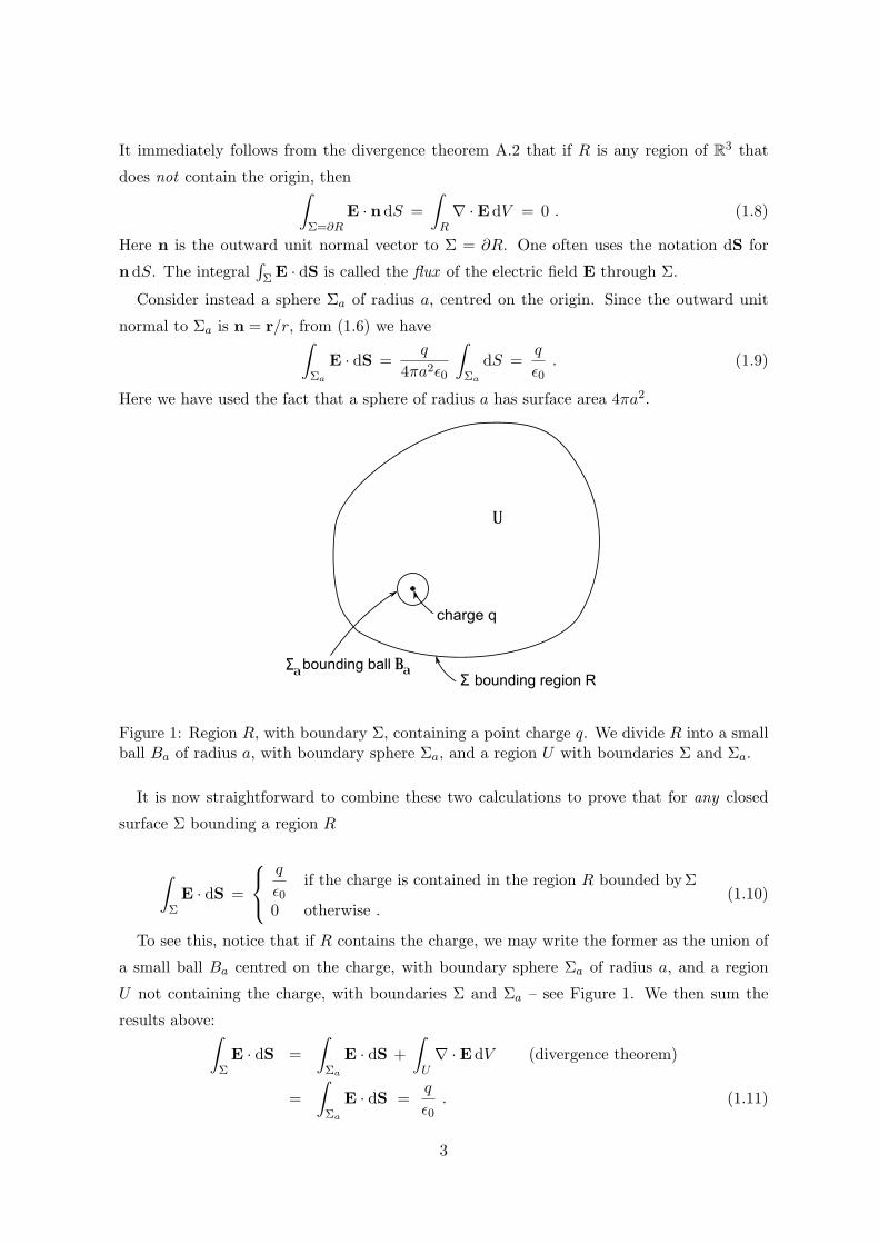
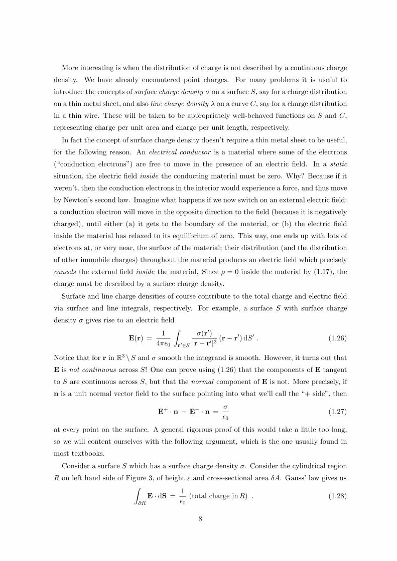
Figure 1: Region R, with boundary Σ, containing a point charge q. We divide R into a smallball Ba of radius a, with boundary sphere Σa, and a region U with boundaries Σ and Σa.
It is now straightforward to combine these two calculations to prove that for any closed
surface Σ bounding a region R
∫
ΣE · dS =
q
ǫ0if the charge is contained in the region R bounded by Σ
0 otherwise .(1.10)
To see this, notice that if R contains the charge, we may write the former as the union of
a small ball Ba centred on the charge, with boundary sphere Σa of radius a, and a region
U not containing the charge, with boundaries Σ and Σa – see Figure 1. We then sum the
results above:∫
ΣE · dS =
∫
Σa
E · dS +
∫
U∇ · EdV (divergence theorem)
=
∫
Σa
E · dS =q
ǫ0. (1.11)
3
This is easily extended to the case of a distribution of multiple point charges. Note first
that the electric field (1.5) has zero divergence on R3 \r1, . . . , rN – the ith term in the sum
has zero divergence on R3 \ ri by the same calculation as (1.7). Suppose that a region R
contains the charges q1, . . . , qm, with m ≤ N . Then one may similarly write R as the union
of m small balls, each containing one charge, and a region containing no charges. For the ith
ball the electric flux calculation (1.9) proceeds in exactly the same way for the ith term in
the sum in (1.5); on the other hand, the remaining terms in the sum have zero divergence in
this ball. Thus essentially the same calculation5 as that above proves
Gauss’ law: For any closed surface Σ bounding a region R,∫
ΣE · dS =
1
ǫ0
m∑
i=1
qi =Q
ǫ0(1.12)
where R contains the point charges q1, . . . , qm, and Q is the total charge in R.
Note that this extension from a single charge to many charges is an application of the
Principle of Superposition, E3 .
1.4 Charge density and Gauss’ law
For many problems it is not convenient to deal with point charges. If the point charges
we have been discussing are, say, electrons, then a macroscopic6 object will consist of an
absolutely enormous number of electrons, each with a very tiny charge. We thus introduce
the concept of charge density ρ(r), which is a function giving the charge per unit volume.
This means that, by definition, the total charge Q = Q(R) in a region R is
Q =
∫
Rρ dV . (1.13)
We shall always assume that the function ρ is sufficiently well-behaved, for example at least
continuous (although see the starred section below). For the purposes of physical arguments,
we shall often think of the Riemann integral as the limit of a sum (which is what it is).
Thus, if δR ⊂ R3 is a small region centred around a point r ∈ R
3 in such a sum, that region
contributes a charge ρ(r)δV , where δV is the volume of δR.
With this definition, the obvious limit of the sum in (1.5), replacing a point charge q′ at
position r′ by ρ(r′)δV ′, becomes a volume integral
E(r) =1
4πǫ0
∫
r′∈R
ρ(r′)
|r − r′|3(r − r′) dV ′ . (1.14)
5Make sure that you understand this by writing out the argument carefully.6* A different issue is that, at the microscopic scale, the charge of an electron is not pointlike, but rather
is effectively smeared out into a smooth distribution of charge. In fact in quantum mechanics the preciseposition of an electron cannot be measured in principle!
4
Here r ∈ R3 | ρ(r) 6= 0 ⊂ R, so that all charge is contained in the (usually bounded) region
R. We shall come back to this formula in the next subsection. Similarly, the limit of (1.12)
becomes∫
ΣE · dS =
1
ǫ0
∫
Rρ dV (1.15)
for any region R with boundary ∂R = Σ. Using the divergence theorem A.2 we may rewrite
this as∫
R
(∇ · E −
ρ
ǫ0
)dV = 0 . (1.16)
Since this holds for all R, we conclude from Lemma A.3 another version of Gauss’ law
∇ · E =ρ
ǫ0. (1.17)
We have derived the first of Maxwell’s equations, on the front cover, from the three simple
laws of electrostatics. In fact this equation holds in general, i.e. even when there are magnetic
fields and time dependence.
* If (1.17) is to apply for the density ρ of a point charge, say at the origin, notice that(1.7) implies that ρ = 0 on R
3 \ 0, but still the integral of ρ over a neighbourhoodof the origin is non-zero. This is odd behaviour for a function. In fact ρ for a pointcharge is a Dirac delta function centred at the point, which is really a “distribution”, ora “generalized function”, rather than a function. Unfortunately we will not have time todiscuss this further here – curious readers may consult page 26 of the book by Jackson,listed in the bibliography. When writing a charge density ρ we shall generally assume itis at least continuous. Thus if one has a continuous charge distribution described by sucha ρ, but also point charges are present, then one must add the point charge contribution(1.5) to (1.14) to obtain the total electric field.
1.5 The electrostatic potential and Poisson’s equation
Returning to our point charge (1.6) again, note that
E = −∇φ (1.18)
where
φ(r) =q
4πǫ0r. (1.19)
Since the curl of a gradient is identically zero, we have
∇∧ E = 0 . (1.20)
Equation (1.20) is another of Maxwell’s equations from the front cover, albeit only in the
special case where ∂B/∂t = 0 (the magnetic field is time-independent).
5
Strictly speaking, we have shown this is valid only on R3 \0 for a point charge. However,
for a bounded continuous charge density ρ(r), with support r ∈ R3 | ρ(r) 6= 0 ⊂ R with R
a bounded region, we may define
φ(r) =1
4πǫ0
∫
r′∈R
ρ(r′)
|r − r′|dV ′ . (1.21)
Theorem A.4 then implies that φ is differentiable with −∇φ = E given by (1.14). The proof
of this goes as follows. Notice first that
∇
(1
|r − r′|
)= −
r − r′
|r − r′|3, r 6= r′ . (1.22)
Hence7
−∇φ(r) =1
4πǫ0
∫
r′∈R
[−∇
(1
|r − r′|
)]ρ(r′) dV ′
=1
4πǫ0
∫
r′∈R
ρ(r′)(r − r′)
|r − r′|3dV ′ = E(r) . (1.23)
Theorem A.4 also states that if ρ(r) is differentiable then ∇φ = −E is differentiable. Since E
is a gradient its curl is identically zero, and we thus deduce that the Maxwell equation (1.20)
is valid on R3.
* In fact ∇ ∧ E = 0 implies that the vector field E is the gradient of a function (1.18),provided the domain of definition has simple enough topology. For example, this is truein R
3 or in an open ball. For other domains, such as R3 minus a line (say, the z-axis), it
is not always possible to write a vector field E with zero curl as a gradient. A systematicdiscussion of this is certainly beyond this course. The interested reader can find a prooffor an open ball in appendix B of the book by Prof Woodhouse listed in the Bibliography.From now on we always assume that E is a gradient (1.18), which in particular will betrue if we work on the whole of R
3 or an open ball.
The function φ is called the electrostatic potential. Recall from Moderations that forces F
which are gradients are called conservative forces. Since F = q E, we see that the electrostatic
force is conservative. The work done against the electrostatic force in moving a charge q along
a curve C is then the line integral
W = −
∫
CF · dr = −q
∫
CE · dr = q
∫
C∇φ · dr = q (φ(r1) − φ(r0)) . (1.24)
Here the curve C begins at r0 and ends at r1. The work done is of course independent of
the choice of curve connecting the two points, because the force is conservative. Notice that
one may add a constant to φ without changing E. It is only the difference in values of φ
that is physical, and this is called the voltage. If we fix some arbitrary point r0 and choose
7One should worry about what happens when r ∈ R, since 1/|r − r′| diverges at r
′ = r. However, thesteps above are nevertheless correct as stated – see the proof of Theorem A.4 in the lecture course “Calculusin Three Dimensions and Applications” for details.
6
φ(r0) = 0, then φ(r) has the interpretation of work done against the electric field in moving a
unit charge from r0 to r. Note that φ in (1.19) is zero “at infinity”. From the usual relation
between work and energy, φ is also the potential energy per unit charge.
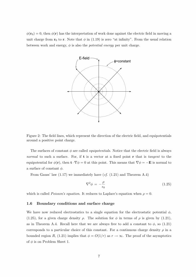
Figure 2: The field lines, which represent the direction of the electric field, and equipotentialsaround a positive point charge.
The surfaces of constant φ are called equipotentials. Notice that the electric field is always
normal to such a surface. For, if t is a vector at a fixed point r that is tangent to the
equipotential for φ(r), then t · ∇φ = 0 at this point. This means that ∇φ = −E is normal to
a surface of constant φ.
From Gauss’ law (1.17) we immediately have (cf. (1.21) and Theorem A.4)
∇2φ = −ρ
ǫ0(1.25)
which is called Poisson’s equation. It reduces to Laplace’s equation when ρ = 0.
1.6 Boundary conditions and surface charge
We have now reduced electrostatics to a single equation for the electrostatic potential φ,
(1.25), for a given charge density ρ. The solution for φ in terms of ρ is given by (1.21),
as in Theorem A.4. Recall here that we are always free to add a constant to φ, so (1.21)
corresponds to a particular choice of this constant. For a continuous charge density ρ in a
bounded region R, (1.21) implies that φ = O(1/r) as r → ∞. The proof of the asymptotics
of φ is on Problem Sheet 1.
7
More interesting is when the distribution of charge is not described by a continuous charge
density. We have already encountered point charges. For many problems it is useful to
introduce the concepts of surface charge density σ on a surface S, say for a charge distribution
on a thin metal sheet, and also line charge density λ on a curve C, say for a charge distribution
in a thin wire. These will be taken to be appropriately well-behaved functions on S and C,
representing charge per unit area and charge per unit length, respectively.
In fact the concept of surface charge density doesn’t require a thin metal sheet to be useful,
for the following reason. An electrical conductor is a material where some of the electrons
(“conduction electrons”) are free to move in the presence of an electric field. In a static
situation, the electric field inside the conducting material must be zero. Why? Because if it
weren’t, then the conduction electrons in the interior would experience a force, and thus move
by Newton’s second law. Imagine what happens if we now switch on an external electric field:
a conduction electron will move in the opposite direction to the field (because it is negatively
charged), until either (a) it gets to the boundary of the material, or (b) the electric field
inside the material has relaxed to its equilibrium of zero. This way, one ends up with lots of
electrons at, or very near, the surface of the material; their distribution (and the distribution
of other immobile charges) throughout the material produces an electric field which precisely
cancels the external field inside the material. Since ρ = 0 inside the material by (1.17), the
charge must be described by a surface charge density.
Surface and line charge densities of course contribute to the total charge and electric field
via surface and line integrals, respectively. For example, a surface S with surface charge
density σ gives rise to an electric field
E(r) =1
4πǫ0
∫
r′∈S
σ(r′)
|r − r′|3(r − r′) dS′ . (1.26)
Notice that for r in R3 \S and σ smooth the integrand is smooth. However, it turns out that
E is not continuous across S! One can prove using (1.26) that the components of E tangent
to S are continuous across S, but that the normal component of E is not. More precisely, if
n is a unit normal vector field to the surface pointing into what we’ll call the “+ side”, then
E+ · n − E− · n =σ
ǫ0(1.27)
at every point on the surface. A general rigorous proof of this would take a little too long,
so we will content ourselves with the following argument, which is the one usually found in
most textbooks.
Consider a surface S which has a surface charge density σ. Consider the cylindrical region
R on left hand side of Figure 3, of height ε and cross-sectional area δA. Gauss’ law gives us∫
∂RE · dS =
1
ǫ0(total charge inR) . (1.28)
8
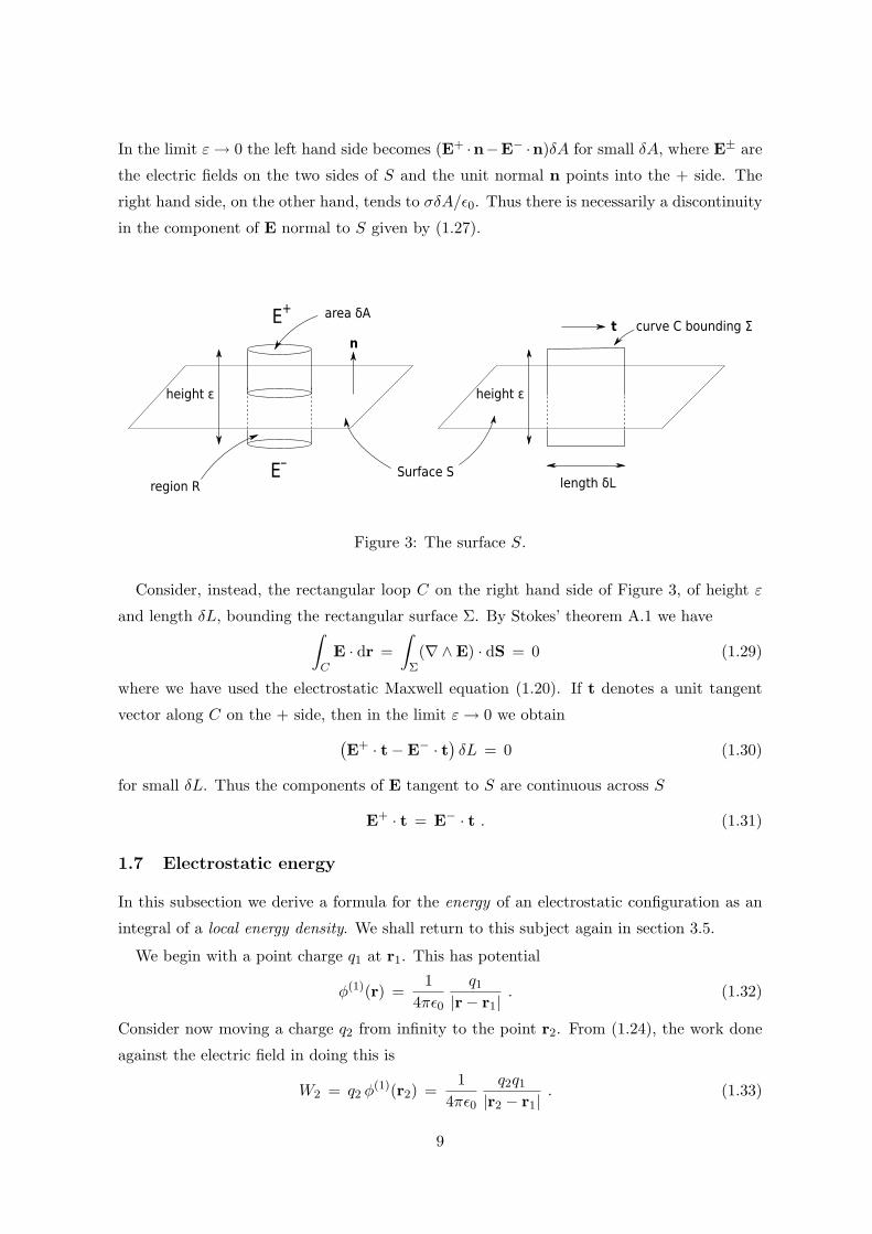
In the limit ε → 0 the left hand side becomes (E+ ·n−E− ·n)δA for small δA, where E± are
the electric fields on the two sides of S and the unit normal n points into the + side. The
right hand side, on the other hand, tends to σδA/ǫ0. Thus there is necessarily a discontinuity
in the component of E normal to S given by (1.27).
Figure 3: The surface S.
Consider, instead, the rectangular loop C on the right hand side of Figure 3, of height ε
and length δL, bounding the rectangular surface Σ. By Stokes’ theorem A.1 we have∫
CE · dr =
∫
Σ(∇∧ E) · dS = 0 (1.29)
where we have used the electrostatic Maxwell equation (1.20). If t denotes a unit tangent
vector along C on the + side, then in the limit ε → 0 we obtain
(E+ · t − E− · t
)δL = 0 (1.30)
for small δL. Thus the components of E tangent to S are continuous across S
E+ · t = E− · t . (1.31)
1.7 Electrostatic energy
In this subsection we derive a formula for the energy of an electrostatic configuration as an
integral of a local energy density. We shall return to this subject again in section 3.5.
We begin with a point charge q1 at r1. This has potential
φ(1)(r) =1
4πǫ0
q1
|r − r1|. (1.32)
Consider now moving a charge q2 from infinity to the point r2. From (1.24), the work done
against the electric field in doing this is
W2 = q2 φ(1)(r2) =1
4πǫ0
q2q1
|r2 − r1|. (1.33)
9
Next move in another charge q3 from infinity to the point r3. We must now do work against
the electric fields of both q1 and q2. By the Principle of Superposition, this work done is
W3 =1
4πǫ0
(q3q1
|r3 − r1|+
q3q2
|r3 − r2|
). (1.34)
The total work done so far is thus W2 + W3.
Obviously, we may continue this process and inductively deduce that the total work done
in assembling charges q1, . . . , qN at r1, . . . , rN is
W =1
4πǫ0
N∑
i=1
∑
j<i
qiqj
|ri − rj |=
1
2·
1
4πǫ0
N∑
i=1
∑
j 6=i
qiqj
|ri − rj |. (1.35)
This is also the potential energy of the collection of charges.
We now rewrite (1.35) as
W =1
2
N∑
i=1
qi φi (1.36)
where we have defined
φi =1
4πǫ0
∑
j 6=i
qj
|ri − rj |. (1.37)
This is simply the electrostatic potential produced by all but the ith charge, evaluated at
position ri. In the usual continuum limit, (1.36) becomes
W =1
2
∫
Rρ φdV (1.38)
where φ(r) is given by (1.21). Now, using Gauss’ law (1.17) we may write
φρ
ǫ0= φ∇ · E = ∇ · (φE) −∇φ · E = ∇ · (φE) + E · E , (1.39)
where in the last step we used (1.18). Inserting this into (1.38), we have
W =ǫ02
[∫
Σ=∂RφE · dS +
∫
RE · EdV
](1.40)
where we have used the divergence theorem on the first term. Taking R to be a very large
ball of radius r, enclosing all charge, the surface Σ is a sphere. For boundary conditions8
φ = O(1/r) as r → ∞, this surface term is zero in the limit that the ball becomes infinitely
large, and we deduce the important formula
W =ǫ02
∫
R3
E · EdV . (1.41)
When this integral exists the configuration is said to have finite energy. The formula (1.41)
suggests that the energy is stored in a local energy density
U =ǫ02
E · E =ǫ02|E|2 . (1.42)
8See Problem Sheet 1, question 3.
10
2 Magnetostatics
2.1 Electric currents
So far we have been dealing with stationary charges. In this subsection we consider how to
describe charges in motion.
Consider, for example, an electrical conductor. In such a material there are electrons (the
“conduction electrons”) which are free to move when an external electric field is applied.
Although these electrons move around fairly randomly, with typically large velocities, in the
presence of a macroscopic electric field there is an induced average drift velocity v = v(r).
This is the average velocity of a particle at position r. In fact, we might as well simply ignore
the random motion, and regard the electrons as moving through the material with velocity
vector field v(r).
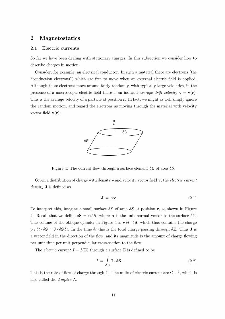
Figure 4: The current flow through a surface element δΣ of area δS.
Given a distribution of charge with density ρ and velocity vector field v, the electric current
density J is defined as
J = ρv . (2.1)
To interpret this, imagine a small surface δΣ of area δS at position r, as shown in Figure
4. Recall that we define δS = n δS, where n is the unit normal vector to the surface δΣ.
The volume of the oblique cylinder in Figure 4 is v δt · δS, which thus contains the charge
ρv δt · δS = J · δS δt. In the time δt this is the total charge passing through δΣ. Thus J is
a vector field in the direction of the flow, and its magnitude is the amount of charge flowing
per unit time per unit perpendicular cross-section to the flow.
The electric current I = I(Σ) through a surface Σ is defined to be
I =
∫
ΣJ · dS . (2.2)
This is the rate of flow of charge through Σ. The units of electric current are C s−1, which is
also called the Ampere A.
11
2.2 The continuity equation
An important property of electric charge is that it is conserved, i.e. it is neither created nor
destroyed. There is a differential equation that expresses this experimental fact called the
continuity equation.
Suppose that Σ is a closed surface bounding a region R, so ∂R = Σ. From the discussion
of current density J in the previous subsection, we see that the rate of flow of electric charge
passing out of Σ is given by the current (2.2) through Σ. On the other hand, the total charge
in R is
Q =
∫
Rρ dV . (2.3)
If electric charge is conserved, then the rate of charge passing out of Σ must equal minus the
rate of change of Q:
∫
ΣJ · dS = −
dQ
dt= −
∫
R
∂ρ
∂tdV . (2.4)
Here we have allowed time dependence in ρ = ρ(r, t). Using the divergence theorem A.2 this
becomes
∫
R
(∂ρ
∂t+ ∇ · J
)dV = 0 (2.5)
for all R, and thus
∂ρ
∂t+ ∇ · J = 0 . (2.6)
This is the continuity equation.
In magnetostatics we shall impose ∂ρ/∂t = 0, and thus
∇ · J = 0 . (2.7)
Such currents are called steady currents.
2.3 The Lorentz force and the magnetic field
The force on a point charge q at rest in an electric field E is simply F = q E. We used this
to define E in fact.
When the charge is moving the force law is more complicated. From experiments one finds
that if q at position r is moving with velocity u = dr/dt it experiences a force
F = q E(r) + q u ∧ B(r) . (2.8)
12
Here B = B(r) is a vector field, called the magnetic field, and we may similarly regard the
Lorentz force F in (2.8) as defining B. The magnetic field is measured in SI units in Teslas,
which is the same as N s m−1 C−1.
Since (2.8) may look peculiar at first sight, it is worthwhile discussing it a little further.
The magnetic component may be written as
Fmag = q u ∧ B . (2.9)
In experiments, the magnetic force on q is found to be proportional to q, proportional to
the magnitude |u| of u, and is perpendicular to u. Note this latter point means that the
magnetic force does no work on the charge. One also finds that the magnetic force at each
point is perpendicular to a particular fixed direction at that point, and is also proportional
to the sine of the angle between u and this fixed direction. The vector field that describes
this direction is called the magnetic field B, and the above, rather complicated, experimental
observations are summarized by the simple formula (2.9).
In practice (2.8) was deduced not from moving test charges, but rather from currents in
test wires. A current of course consists of moving charges, and (2.8) was deduced from the
forces on these test wires.
2.4 The Biot-Savart law
If electric charges produce the electric field, what produces the magnetic field? The answer is
that electric currents produce magnetic fields! Note carefully the distinction here: currents
produce magnetic fields, but, by the Lorentz force law just discussed, magnetic fields exert a
force on moving charges, and hence currents.
The usual discussion of this involves currents in wires, since this is what Ampere actually
did in 1820. One has a wire with steady current I flowing through it. Here the latter is
defined in terms of the current density via (2.2), where Σ is any cross-section of the wire.
This is independent of the choice of cross-section, and thus makes sense, because9 of the
steady current condition (2.7). One finds that another wire, the test wire, with current I ′
experiences a force. This force is conveniently summarized by introducing the concept of a
magnetic field: the first wire produces a magnetic field, which generates a force on the second
wire via the Lorentz force (2.8) acting on the charges that make up the current I ′.
Rather than describe this in detail, we shall instead simply note that if currents produce
magnetic fields, then fundamentally it is charges in motion that produce magnetic fields. One
may summarize this by an analogous formula to the Coulomb formula (1.6) for the electric
9use the divergence theorem for a cylindrical region bounded by any two cross-sections and the surface ofthe wire.
13
field due to a point charge. A charge q at the origin with velocity v produces a magnetic field
B(r) =µ0 q
4π
v ∧ r
r3. (2.10)
Here the constant µ0 is called the permeability of free space, and takes the value µ0 = 4π ×
10−7 N s2 C−2. Compare (2.10) to (1.6).
Importantly, we also have that
The magnetic field obeys the Principle of Superposition.
We may easily compute the magnetic field due to the steady current I in a wire C by
summing contributions of the form (2.10):
B(r) =µ0 I
4π
∫
C
dr′ ∧ (r − r′)
|r − r′|3. (2.11)
To see this, imagine dividing the wire into segments, with the segment δr′ at position r′.
Suppose this segment contains a charge q(r′) with velocity vector v(r′) – notice here that
v(r′) points in the same direction as δr′. From (2.10) this segment contributes
δB(r) =µ0 q
4π
v ∧ (r − r′)
|r − r′|3. (2.12)
to the magnetic field. Now by definition of the current I we have I δr′ = ρv · δS δr′, where
we may take δΣ of area δS to be a perpendicular cross-section of the wire. But the total
charge q in the cylinder of cross-sectional area δS and length |δr′| is q = ρ δS |δr′|. We thus
deduce that I δr′ = q v and hence that (2.11) holds.
The formula (2.11) for the magnetic field produced by the steady current in a wire is called
the Biot-Savart law. In fact (2.10) is also often called the Biot-Savart law.
Example: the magnetic field of an infinite straight line current
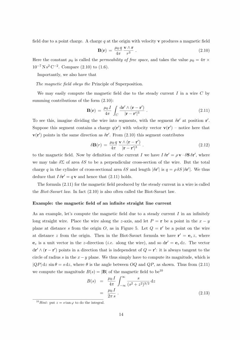
As an example, let’s compute the magnetic field due to a steady current I in an infinitely
long straight wire. Place the wire along the z-axis, and let P = r be a point in the x − y
plane at distance s from the origin O, as in Figure 5. Let Q = r′ be a point on the wire
at distance z from the origin. Then in the Biot-Savart formula we have r′ = ez z, where
ez is a unit vector in the z-direction (i.e. along the wire), and so dr′ = ez dz. The vector
dr′ ∧ (r − r′) points in a direction that is independent of Q = r′: it is always tangent to the
circle of radius s in the x− y plane. We thus simply have to compute its magnitude, which is
|QP |dz sin θ = sdz, where θ is the angle between OQ and QP , as shown. Thus from (2.11)
we compute the magnitude B(s) = |B| of the magnetic field to be10
B(s) =µ0 I
4π
∫ ∞
−∞
s
(s2 + z2)3/2dz
=µ0 I
2π s. (2.13)
10Hint : put z = s tan ϕ to do the integral.
14
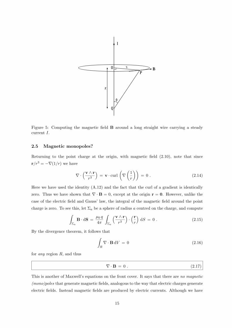
Figure 5: Computing the magnetic field B around a long straight wire carrying a steadycurrent I.
2.5 Magnetic monopoles?
Returning to the point charge at the origin, with magnetic field (2.10), note that since
r/r3 = −∇(1/r) we have
∇ ·(v ∧ r
r3
)= v · curl
(∇
(1
r
))= 0 . (2.14)
Here we have used the identity (A.12) and the fact that the curl of a gradient is identically
zero. Thus we have shown that ∇ · B = 0, except at the origin r = 0. However, unlike the
case of the electric field and Gauss’ law, the integral of the magnetic field around the point
charge is zero. To see this, let Σa be a sphere of radius a centred on the charge, and compute
∫
Σa
B · dS =µ0 q
4π
∫
Σa
(v ∧ r
r3
)·(r
r
)dS = 0 . (2.15)
By the divergence theorem, it follows that
∫
R∇ · B dV = 0 (2.16)
for any region R, and thus
∇ · B = 0 . (2.17)
This is another of Maxwell’s equations on the front cover. It says that there are no magnetic
(mono)poles that generate magnetic fields, analogous to the way that electric charges generate
electric fields. Instead magnetic fields are produced by electric currents. Although we have
15
only deduced (2.17) above for the magnetic field of a moving point charge, the general case
follows from the Principle of Superposition.
You might wonder what produces the magnetic field in permanent magnets, such as bar
magnets. Where is the electric current? It turns out that, in certain magnetic materials, the
macroscopic magnetic field is produced by the alignment of tiny atomic currents generated
by the electrons in the material (in others it is due to the alignment of the “spins” of the
electrons, which is a quantum mechanical property).
* Mathematically, it is certainly possible to allow for magnetic monopoles and magneticcurrents in Maxwell’s equations. In fact the equations then become completely symmetricunder the interchange of E with −cB, cB with E, and corresponding interchanges ofelectric with magnetic sources and currents. Here c2 = 1/ǫ0µ0. There are also theoreticalreasons for introducing magnetic monopoles. For example, the quantization of electriccharge – that all electric charges are an integer multiple of some fixed fundamental quantityof charge – may be understood in quantum mechanics using magnetic monopoles. Thisis a beautiful argument due to Dirac. However, no magnetic monopoles have ever beenobserved in nature. If they existed, (2.17) would need correcting.
2.6 Ampere’s law
There is just one more static Maxwell equation to discuss, and that is the equation involving
the curl of B. This is Ampere’s law. In many treatments of magnetostatics, this is often
described as an additional experimental result, and/or is derived for special symmetric con-
figurations, having first solved for B using the Biot-Savart law (2.10) or (2.11). However, it
is possible to derive Ampere’s law directly from (2.10).
We first use (2.10) and the Principle of Superposition to write B generated by a current
density J as a volume integral
B(r) =µ0
4π
∫
r′∈R
J(r′) ∧ (r − r′)
|r − r′|3dV ′ . (2.18)
This follows directly from the definition J = ρv in (2.1) and taking the limit of a sum of
terms of the form (2.10). R is by definition a region containing the set of points with J 6= 0.
We next define the vector field
A(r) =µ0
4π
∫
R
J(r′)
|r − r′|dV ′ . (2.19)
One easily computes (cf. Theorem A.4 with f = µ0Ji / 4π)
∂Ai
∂xj(r) = −
µ0
4π
∫
R
Ji(r′)
|r − r′|3(xj − x′
j) dV ′ (2.20)
and thus
B(r) = ∇∧ A(r) . (2.21)
16
Note that (2.21) directly implies ∇ · B = 0.
We next take the curl of (2.21). Using
∇∧ (∇∧ A) = ∇(∇ · A) −∇2 A , (2.22)
which holds for any vector field A, we obtain
∇∧ B(r) =µ0
4π∇
[∫
RJ(r′) · ∇
(1
|r − r′|
)dV ′
]− ∇2 A(r) . (2.23)
We first deal with the first term. It is important that the integrand is in fact integrable over a
neighbourhood of r = r′. One can see this using spherical polar coordinates about the point
r – see the proof of Theorem A.4. Now using
∇
(1
|r − r′|
)= −∇′
(1
|r − r′|
), r 6= r′ , (2.24)
where ∇′ denotes derivative with respect to r′, the term in square brackets is∫
RJ(r′) · ∇
(1
|r − r′|
)dV ′ = −
∫
R∇′ ·
(J(r′)
|r − r′|
)dV ′
+
∫
R
1
|r − r′|
(∇′ · J(r′)
)dV ′ . (2.25)
The second term on the right hand side of equation (2.25) is zero for steady currents (2.7).
Moreover, we may use the divergence theorem on the first term to obtain a surface integral
on ∂R. But by assumption J vanishes on this boundary, so this term is also zero.
Thus ∇ · A = 0 and we have shown that
∇∧ B = −∇2 A . (2.26)
We now use Theorem A.4, again with f = µ0Ji / 4π for each component Ji of J, to deduce
∇∧ B = µ0 J . (2.27)
This is Ampere’s law for magnetostatics. It is the final Maxwell equation on the front cover,
albeit in the special case where the electric field is independent of time, so ∂E/∂t = 0. Note
this equation is consistent with the steady current assumption (2.7).
We may equivalently rewrite (2.27) using Stokes’ theorem as
Ampere’s law: For any simple closed curve C = ∂Σ bounding a surface Σ∫
C=∂ΣB · dr = µ0
∫
ΣJ · dS = µ0I (2.28)
where I is the current through Σ.
As an example, notice that integrating the magnetic field B given by (2.13) around a circle
C in the x − y plane of radius s and centred on the z-axis indeed gives µ0I.
17
2.7 The magnetostatic vector potential
In magnetostatics it is possible to introduce a magnetic vector potential A analogous to the
electrostatic potential φ in electrostatics. In fact we have already introduced such a vector
potential in (2.21) and (2.19):
B = ∇∧ A (2.29)
where A is the magnetic vector potential.
* Notice that (2.29) is a sufficient condition for the Maxwell equation (2.17). It is alsonecessary if we work in a domain with simple enough topology, such as R
3 or an open ball.A domain where not every vector field B with zero divergence may be written as a curl isR
3 with a point removed. Compare this to the corresponding starred paragraph in section1.5. Again, a proof for an open ball is contained in appendix B of Prof Woodhouse’s book.
Notice that A in (2.29) is far from unique: since the curl of a gradient is zero, we may add
∇ψ to A, for any function ψ, without changing B:
A → A = A + ∇ψ . (2.30)
This is called a gauge transformation of A. We may fix this gauge freedom by imposing
additional conditions on A. For example, suppose we have chosen a particular A satisfying
(2.29). Then by choosing ψ to be a solution of the Poisson equation
∇2ψ = −∇ · A (2.31)
it follows that A in (2.30) satisfies
∇ · A = 0 . (2.32)
This is called the Lorenz gauge (Mr Lorenz and Mr Lorentz were two different people). As
you learned11 in the Moderations course on vector calculus, the solution to Poisson’s equation
(2.31) is unique for fixed boundary conditions.
Many equations simplify with this choice for A. For example, Ampere’s law (2.27) becomes
µ0 J = ∇∧ (∇∧ A) = ∇(∇ · A) − ∇2 A (2.33)
so that in Lorenz gauge ∇ · A = 0 this becomes
∇2 A = −µ0 J . (2.34)
Compare with Poisson’s equation (1.25) in electrostatics. Notice that we showed in the
previous subsection that A in (2.19) is in Lorenz gauge.
* Gauge invariance and the vector potential A play a fundamental role in more advancedformulations of electromagnetism. The magnetic potential also plays an essential physicalrole in the quantum theory of electromagnetism.
11Corollary 7.3.
18
3 Electrodynamics and Maxwell’s equations
3.1 Maxwell’s displacement current
Let’s go back to Ampere’s law (2.28) in magnetostatics∫
C=∂ΣB · dr = µ0
∫
ΣJ · dS . (3.1)
Here C = ∂Σ is a simple closed curve bounding a surface Σ. Of course, one may use any such
surface spanning C on the right hand side. If we pick a different surface Σ′, with C = ∂Σ′,
then
0 =
∫
ΣJ · dS −
∫
Σ′
J · dS
=
∫
SJ · dS . (3.2)
Here S is the closed surface obtained by gluing Σ and Σ′ together along C. Thus the flux of
J through any closed surface is zero. We may see this in a different way if we assume that
S = ∂R bounds a region R, since then∫
SJ · dS =
∫
R∇ · J dV = 0 (3.3)
and in the last step we have used the steady current condition (2.7).
But in general, (2.7) should be replaced by the continuity equation (2.6). The above
calculation then changes to∫
ΣJ · dS −
∫
Σ′
J · dS =
∫
SJ · dS
=
∫
R∇ · J dV
= −
∫
R
∂ρ
∂tdV
= −ǫ0
∫
R
∂
∂t(∇ · E) dV
= −ǫ0
∫
S=∂R
∂E
∂t· dS
= −ǫ0
∫
Σ
∂E
∂t· dS + ǫ0
∫
Σ′
∂E
∂t· dS . (3.4)
Notice we have used Gauss’ law (1.17), and that we now regard E = E(r, t) as a vector field
depending on time. This shows that∫
Σ
(J + ǫ0
∂E
∂t
)· dS =
∫
Σ′
(J + ǫ0
∂E
∂t
)· dS (3.5)
for any two surfaces Σ, Σ′ spanning C, and thus suggests replacing Ampere’s law (2.27) by
∇∧ B = µ0
(J + ǫ0
∂E
∂t
). (3.6)
19
This is indeed the correct time-dependent Maxwell equation on the front cover. The addi-
tional term ∂E/∂t is called the displacement current. It says that a time-dependent electric
field also produces a magnetic field.
3.2 Faraday’s law
The electrostatic equation (1.20) is also modified in the time-dependent case. We can motivate
how precisely by the following argument. Consider the electromagnetic field generated by a
set of charges all moving with constant velocity v. The charges generate both an E and a B
field, the latter since the charges are in motion. However, consider instead an observer who
is also moving at the same constant velocity v. For this observer, the charges are at rest, and
thus he/she will measure only an electric field E′ from the Lorentz force law (2.8) on one of
the charges! Since (or assuming) the two observers must be measuring the same force on a
given charge, we conclude that
E′ = E + v ∧ B . (3.7)
Now since the field is electrostatic for the moving observer,
0 = ∇∧ E′
= ∇∧ E + ∇∧ (v ∧ B)
= ∇∧ E + v(∇ · B) − (v · ∇)B
= ∇∧ E − (v · ∇)B . (3.8)
Here we have used the identity (A.11), and in the last step we have used ∇ · B = 0. Now,
for the original observer the charges are all moving with velocity v, so the magnetic field at
position r + vτ and time t + τ is the same as that at position r and time t:
B(r + vτ, t + τ) = B(r, t) . (3.9)
This implies the partial differential equation
(v · ∇)B +∂B
∂t= 0 (3.10)
and we deduce from (3.8) that
∇∧ E = −∂B
∂t. (3.11)
This is Faraday’s law, and is another of Maxwell’s equations. The above argument raises
issues about what happens in general to our equations when we change to a moving frame.
This is not something we want to pursue further here, because it leads to Einstein’s theory
20
of Special Relativity ! This will be studied further in the Part B course on Special Relativity
and Electromagnetism.
As usual, the equation (3.11) may be expressed as an integral equation as
Faraday’s law: For any simple closed curve C = ∂Σ bounding a fixed surface Σ
∫
C=∂ΣE · dr = −
d
dt
∫
ΣB · dS . (3.12)
This says that a time-dependent magnetic field produces an electric field. For example,
if one moves a bar magnet through a loop of conducting wire C, the resulting electric field
from (3.11) induces a current in the wire via the Lorentz force. This is what Faraday did, in
fact, in 1831. The integral∫Σ B · dS is called the magnetic flux through Σ.
* The current in the wire then itself produces a magnetic field of course, via Ampere’slaw. However, the signs are such that this magnetic field is in the opposite direction to thechange in the magnetic field that created it. This is called Lenz’s law. The whole setupmay be summarized as follows:
changing BFaraday−→ E
Lorentz−→ current
Ampere−→ B . (3.13)
3.3 Maxwell’s equations
We now summarize the full set of Maxwell equations.
There are two scalar equations, namely Gauss’ law (1.17) from electrostatics, and the
equation (2.17) from magnetostatics that expresses the absence of magnetic monopoles:
∇ · E =ρ
ǫ0(3.14)
∇ · B = 0 . (3.15)
Although we discussed these only in the time-independent case, they are in fact true in
general.
The are also two vector equations, namely Faraday’s law (3.11) and Maxwell’s modification
(3.6) of Ampere’s law (2.27) from magnetostatics:
∇∧ E = −∂B
∂t(3.16)
∇∧ B = µ0
(J + ǫ0
∂E
∂t
). (3.17)
21
Together with the Lorentz force law
F = q (E + u ∧ B)
which governs the mechanics, this is all of electromagnetism. Everything else we have dis-
cussed may in fact be derived from these equations.
Maxwell’s equations, for given ρ and J, are 8 equations for 6 unknowns. There must
therefore be two consistency conditions. To see what these are, we compute
∂
∂t(∇ · B) = −∇ · (∇∧ E) = 0 , (3.18)
where we have used (3.16). This is clearly consistent with (3.15). We get something non-
trivial by instead taking the divergence of (3.17), which gives
0 = ∇ · J + ǫ0∂
∂t(∇ · E)
= ∇ · J +∂ρ
∂t, (3.19)
where we have used (3.14). Thus the continuity equation arises as a consistency condition
for Maxwell’s equations: if ρ and J do not satisfy (3.19), there is no solution to Maxwell’s
equations for this choice of charge density and current.
3.4 Electromagnetic potentials and gauge invariance
In the general time-dependent case one can introduce electromagnetic potentials in a similar
way to the static cases. We work in a suitable domain in R3, such as R
3 itself or an open ball
therein, as discussed in previous sections. Since B has zero divergence (3.15), we may again
introduce a vector potential
B = ∇∧ A , (3.20)
where now A = A(r, t). It follows from Faraday’s law that
0 = ∇∧ E +∂B
∂t= ∇∧
(E +
∂A
∂t
). (3.21)
Thus we may introduce a scalar potential φ = φ(r, t) via
E +∂A
∂t= −∇φ . (3.22)
Thus
B = ∇∧ A (3.23)
E = −∇φ −∂A
∂t. (3.24)
22
Notice that we similarly have the gauge transformations
A → A + ∇ψ, φ → φ −∂ψ
∂t(3.25)
leaving (3.23) and (3.24) invariant. Again, one may fix this non-uniqueness of A and φ by
imposing certain gauge choices. This will be investigated further in Problem Sheet 2. Note
that, by construction, with (3.23) and (3.24) the Maxwell equations (3.15) and (3.16) are
automatically satisfied.
3.5 Electromagnetic energy and Poynting’s theorem
Recall that in section 1.7 we derived a formula for the electrostatic energy density Uelectric =
ǫ0 |E|2 / 2 in terms of the electric field E. The electrostatic energy of a given configuration is
the integral of this density over space (1.41). One can motivate the similar formula Umagnetic =
|B|2 / 2µ0 in magnetostatics, although unfortunately we won’t have time to derive this here.
A natural candidate for the electromagnetic energy density in general is thus
U =ǫ02|E|2 +
1
2µ0|B|2 . (3.26)
Consider taking the partial derivative of (3.26) with respect to time:
∂U
∂t= ǫ0 E ·
∂E
∂t+
1
µ0B ·
∂B
∂t
=1
µ0E · (∇∧ B − µ0 J) −
1
µ0B · (∇∧ E)
= −∇ ·
(1
µ0E ∧ B
)− E · J . (3.27)
Here after the first step we have used the Maxwell equations (3.17) and (3.16), respectively.
The last step uses the identity (A.12). If we now define the Poynting vector P to be
P =1
µ0E ∧ B (3.28)
then we have derived Poynting’s theorem
∂U
∂t+ ∇ · P = −E · J . (3.29)
Notice that, in the absence of a source current, J = 0, this takes the form of a continuity
equation, analogous to the continuity equation (2.6) that expresses conservation of charge. It
is thus natural to interpret (3.29) as a conservation of energy equation, and so identify the
Poynting vector P as some kind of rate of energy flow density. One can indeed justify this
by examining the above quantities in various physical applications.
Integrating (3.29) over a region R with boundary Σ we obtain
d
dt
∫
RU dV = −
∫
ΣP · dS −
∫
RE · J dV . (3.30)
23
Given our discussion of U , the left hand side is clearly the rate of increase of energy in R.
The first term on the right hand side is the rate of energy flow into the region R. When
J = 0, this is precisely analogous to our discussion of charge conservation in section 2.2.
The final term in (3.30) is interpreted as (minus) the rate of work by the field on the sources.
To see this, remember that the force on a charge q moving at velocity v is F = q (E + v∧B).
This force does work at a rate given by F · v = q E · v. Recalling the definition (2.1) of
J = ρv, we see that the force does work on the charge q = ρ δV in a small volume δV at a
rate F · v = E · J δV .
4 Electromagnetic waves
4.1 Source-free equations and electromagnetic waves
We begin by writing down Maxwell’s equations in vacuum, where there is no electric charge
or current present:
∇ · E = 0 (4.1)
∇ · B = 0 (4.2)
∇∧ E +∂B
∂t= 0 (4.3)
∇∧ B −1
c2
∂E
∂t= 0 (4.4)
where we have defined
c =
√1
ǫ0 µ0. (4.5)
If you look back at the units of ǫ0 and µ0, you’ll see that ǫ0 µ0 has units (C2 N−1 m−2) ·
(N s2 C−2) = (m s−1)−2. Thus c is a speed. The great insight of Maxwell was to realise it is
the speed of light in vacuum.
Taking the curl of (4.3) we have
0 = ∇(∇ · E) − ∇2 E + ∇∧∂B
∂t
= −∇2 E +∂
∂t(∇∧ B)
= −∇2 E +1
c2
∂2E
∂t2. (4.6)
Here after the first step we have used (4.1), and in the last step we have used (4.4). It follows
that each component of E satisfies the wave equation
2 u = 0 (4.7)
24
where u = u(r, t), and we have defined the d’Alembertian operator
2 =1
c2
∂2
∂t2−∇2 . (4.8)
You can easily check that B also satisfies 2B = 0.
The equation (4.7) governs the propagation of waves of speed c in three-dimensional space.
It is the natural generalization of the one-dimensional wave equation
1
c2
∂2u
∂t2−
∂2u
∂x2= 0 , (4.9)
which you met in the Moderations courses “Fourier Series and Two Variable Calculus”, and
“Partial Differential Equations in Two Dimensions and Applications”. Recall that this has
particular solutions of the form u±(x, t) = f(x ∓ ct), where f is any function which is twice
differentiable. In this case, the waves look like the graph of f travelling at constant velocity
c in the direction of increasing/decreasing x, respectively. The general12 solution to (4.9) is
u(x, t) = f(x − ct) + g(x + ct).
This naturally generalizes to the three-dimensional equation (4.7), by writing
u(r, t) = f(e · r − ct) (4.10)
where e is a fixed unit vector, |e|2 = 1. Indeed, note that ∇2 u = e · e f ′′, ∂2u/∂t2 = c2 f ′′.
Solutions of the form (4.10) are called plane-fronted waves, since at any constant time, u is
constant on the planes e · r = constant orthogonal to e. As time t increases, these plane
wavefronts propagate in the direction of e at speed c. However, unlike the one-dimensional
equation, we cannot write the general solution to (4.7) as a sum of two plane-fronted waves
travelling in opposite directions.
4.2 Monochromatic plane waves
An important special class of plane-fronted waves (4.10) are given by the real harmonic waves
u(r, t) = α cos Ω(r, t) + β sinΩ(r, t) (4.11)
where α, β are constants, and we define
Ω(r, t) =ω
c(ct − e · r) (4.12)
where ω > 0 is the constant frequency of the wave. In fact it is a result of Fourier analysis
that every solution to the wave equation (4.7) is a linear combination (in general involving
an integral) of these harmonic waves.
12see the Mods course on PDEs referred to above.
25
Since the components of E (and B) satisfy (4.7), it is natural to look for solutions of the
harmonic wave form
E(r, t) = α cosΩ(r, t) + β sinΩ(r, t) (4.13)
where α, β are constant vectors, and Ω = Ω(r, t) is again given by (4.12). This of course
satisfies the wave equation, but we must ensure that we satisfy all of the Maxwell equations
in vacuum. The first (4.1) implies
0 = ∇ · E =ω
c(e · α sinΩ − e · β cos Ω) (4.14)
which implies that
e · α = e · β = 0 , (4.15)
i.e. the E-field is orthogonal to the direction of propagation e. Next we look at (4.3):
−∂B
∂t= ∇∧ E =
ω
c(e ∧ α sinΩ − e ∧ β cos Ω) . (4.16)
We may satisfy this equation by taking
B(r, t) =1
ce ∧ E(r, t) =
1
c[e ∧ α cos Ω(r, t) + e ∧ β sinΩ(r, t)] . (4.17)
It is now simple to verify that the last two Maxwell equations (4.2), (4.4) are satisfied by
(4.13), (4.17) – the calculation is analogous to that above, so I leave this as a short exercise.
Notice that the B-field (4.17) is orthogonal to both E and the direction of propagation.
The solution to Maxwell’s equations with E and B given by (4.13), (4.17) is called a
monochromatic electromagnetic plane wave. It is specified by the constant direction of prop-
agation e, |e|2 = 1, two constant vectors α, β orthogonal to this direction, e · α = e · β = 0,
and the frequency ω. Again, using Fourier analysis one can show that the general vacuum
solution is a combination of these monochromatic plane waves.
Notice from the first equality in (4.17) that the Poynting vector (3.28) for a monochromatic
plane wave is
P =1
µ0c|E|2 e =
√ǫ0µ0
|α cos Ω + β sin Ω|2 e (4.18)
which is in the direction of propagation of the wave. Thus electromagnetic waves carry energy,
a fact which anyone who has made a mircowave pot noodle can confirm.
4.3 Polarization
Consider a monochromatic plane wave with E given by (4.13). If we fix a particular point in
space, say the origin r = 0, then
E(0, t) = α cos (ωt) + β sin (ωt) . (4.19)
26
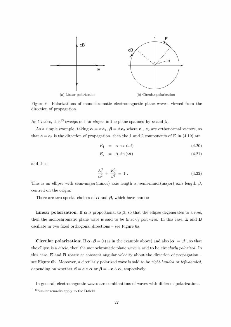
(a) Linear polarization (b) Circular polarization
Figure 6: Polarizations of monochromatic electromagnetic plane waves, viewed from thedirection of propagation.
As t varies, this13 sweeps out an ellipse in the plane spanned by α and β.
As a simple example, taking α = α e1, β = β e2 where e1, e2 are orthonormal vectors, so
that e = e3 is the direction of propagation, then the 1 and 2 components of E in (4.19) are
E1 = α cos (ωt) (4.20)
E2 = β sin (ωt) (4.21)
and thus
E21
α2+
E22
β2= 1 . (4.22)
This is an ellipse with semi-major(minor) axis length α, semi-minor(major) axis length β,
centred on the origin.
There are two special choices of α and β, which have names:
Linear polarization: If α is proportional to β, so that the ellipse degenerates to a line,
then the monochromatic plane wave is said to be linearly polarized. In this case, E and B
oscillate in two fixed orthogonal directions – see Figure 6a.
Circular polarization: If α ·β = 0 (as in the example above) and also |α| = |β|, so that
the ellipse is a circle, then the monochromatic plane wave is said to be circularly polarized. In
this case, E and B rotate at constant angular velocity about the direction of propagation –
see Figure 6b. Moreover, a circularly polarized wave is said to be right-handed or left-handed,
depending on whether β = e ∧ α or β = −e ∧ α, respectively.
In general, electromagnetic waves are combinations of waves with different polarizations.
13Similar remarks apply to the B-field.
27
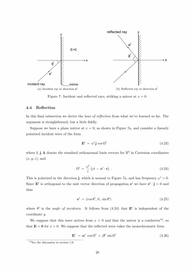
(a) Incident ray in direction ei (b) Reflected ray in direction e
r
Figure 7: Incident and reflected rays, striking a mirror at x = 0.
4.4 Reflection
In this final subsection we derive the laws of reflection from what we’ve learned so far. The
argument is straightfoward, but a little fiddly.
Suppose we have a plane mirror at x = 0, as shown in Figure 7a, and consider a linearly
polarized incident wave of the form
Ei = αi j cos Ωi (4.23)
where i, j, k denote the standard orthonormal basis vectors for R3 in Cartesian coordinates
(x, y, z), and
Ωi =ωi
c
(ct − ei · r
). (4.24)
This is polarized in the direction j, which is normal to Figure 7a, and has frequency ωi > 0.
Since Ei is orthogonal to the unit vector direction of propagation ei we have ei · j = 0 and
thus
ei = (cos θi, 0 , sin θi) (4.25)
where θi is the angle of incidence. It follows from (4.24) that Ei is independent of the
coordinate y.
We suppose that this wave arrives from x < 0 and that the mirror is a conductor14, so
that E = 0 for x > 0. We suppose that the reflected wave takes the monochromatic form
Er = αr cos Ωr + βr sinΩr (4.26)
14See the discussion in section 1.6.
28
where
Ωr =ωr
c(ct − er · r) . (4.27)
The total electric field is thus
E = Ei + Er . (4.28)
From the boundary conditions deduced in section 1.6, we know15 that the components of
E = Ei + Er parallel to the boundary surface at x = 0 are continuous across the surface.
Thus at x = 0
(Ei + Er
)· j |x=0 = 0 (4.29)
(Ei + Er
)· k |x=0 = 0 . (4.30)
Notice from (4.29) that Er · j 6= 0 identically, as otherwise from (4.23) Ei = 0. Since Ei is
independent of y, it thus follows from (4.29) that so is Er, and hence er · j = 0. That is,
R1 : The incident ray, normal, and reflected ray are coplanar.
This is the first law of reflection. We may now write
er = (− cos θr, 0 , sin θr) (4.31)
with θr the angle of reflection, as shown in Figure 7b.
We next define αr = αr · j, βr = βr · j, so that
E · j = αi cos Ωi + αr cosΩr + βr sinΩr . (4.32)
By (4.29), this must vanish at x = 0. In fact, if we further put z = 0 then Ωi = ωi t, Ωr = ωr t,
and thus
f(t) ≡ E · j |x=z=0 = αi cos ωi t + αr cos ωr t + βr sinωr t = 0 . (4.33)
This is to hold for all t. Hence
f(0) = 0 ⇒ αi + αr = 0 (4.34)
f(0) = 0 ⇒ βr = 0 (4.35)
f(0) = 0 ⇒ (ωi)2 αi + (ωr)2 αr = 0 . (4.36)
Combining (4.34) and (4.36) implies ωi = ωr ≡ ω, and thus
15The alert reader will notice that the derivation in section 1.6 was for electrostatics. However, the sameformula (1.31) holds in general. To see this, one notes that the additional surface integral of ∂B/∂t in (1.29)tends to zero as ε → 0.
29
The reflected frequency (colour) is the same as the incident frequency (colour).
We have now reduced (4.29) to
α[cos
ω
c
(ct − z sin θi
)− cos
ω
c(ct − z sin θr)
]= 0 , (4.37)
where α ≡ αi. Thus sin θi = sin θr. Hence θi = θr ≡ θ and we have shown
R2 : The angle of incidence is equal to the angle of reflection.
This is the second law of reflection.
Finally, note that (4.30) is simply Er ·k = 0. Since Er · er = 0, from (4.31) we see that Er
is parallel16 to j. Hence
The reflected wave has the same polarization as the incident wave.
The final form of E (for x < 0) is then computed to be
E = 2α sin[ω
c(ct − z sin θ)
]sin
[ω
cx cos θ
]j . (4.38)
16Note this follows only if θ 6= π/2. If θ = π/2 the waves are propagating parallel to the mirror, in thez-direction.
30
A Summary: vector calculus
The following is a summary of some of the key results of the Moderations course “Calculus in
Three Dimensions and Applications”. As in the main text, all functions and vector fields are
assumed to be sufficiently well-behaved in order for formulae to make sense. For example,
one might take everything to be smooth (derivatives to all orders exist). Similar remarks
apply to (the parametrizations of) curves and surfaces in R3.
A.1 Vectors in R3
We work in R3, or a domain therein, in Cartesian coordinates. If e1 = i = (1, 0, 0), e2 = j =
(0, 1, 0), e3 = k = (0, 0, 1) denote the standard orthonormal basis vectors, then a position
vector is
r =3∑
i=1
xi ei (A.1)
where x1 = x, x2 = y, x3 = z are the Cartesian coordinates in this basis. We denote the
Euclidean length of r by
|r| = r =√
x21 + x2
2 + x23 (A.2)
so that r = r/r is a unit vector for r 6= 0. A vector field f = f(r) may be written in this basis
as
f(r) =3∑
i=1
fi(r) ei . (A.3)
The scalar product of two vectors a, b is denoted by
a · b =3∑
i=1
aibi (A.4)
while their vector product is the vector
a ∧ b = (a2b3 − a3b2) e1 + (a3b1 − a1b3) e2 + (a1b2 − a2b1) e3 . (A.5)
A.2 Vector operators
The gradient of a function ψ = ψ(r) is the vector field
gradψ = ∇ψ =3∑
i=1
∂ψ
∂xiei . (A.6)
The divergence of a vector field f = f(r) is the function (scalar field)
div f = ∇ · f =
3∑
i=1
ei ·∂f
∂xi=
3∑
i=1
∂fi
∂xi(A.7)
I
while the curl is the vector field
curl f = ∇∧ f =3∑
i=1
ei ∧∂f
∂xi
=
(∂f3
∂x2−
∂f2
∂x3
)e1 +
(∂f1
∂x3−
∂f3
∂x1
)e2 +
(∂f2
∂x1−
∂f1
∂x2
)e3 . (A.8)
Two important identities are
∇∧ (∇ψ) = 0 (A.9)
∇ · (∇∧ f) = 0 . (A.10)
Two more identities we shall need are
∇∧ (a ∧ b) = a(∇ · b) − b(∇ · a) + (b · ∇)a − (a · ∇)b , (A.11)
∇ · (a ∧ b) = b · (∇∧ a) − a · (∇∧ b) . (A.12)
The second order operator ∇2 defined by
∇2ψ = ∇ · (∇ψ) =3∑
i=1
∂2ψ
∂x2i
(A.13)
is called the Laplacian. We shall also use the identity
∇∧ (∇∧ f) = ∇ (∇ · f) − ∇2f . (A.14)
A.3 Integral theorems
Definition (Line integral) Let C be a curve in R3, parametrized by r : [t0, t1] → R
3, or r(t)
for short. Then the line integral of a vector field f along C is
∫
Cf · dr =
∫ t1
t0
f(r(t)) ·dr(t)
dtdt . (A.15)
Note that τ (t) = dr/dt is the tangent vector to the curve – a vector field on C. The value
of the integral is independent of the choice of oriented parametrization (proof uses the chain
rule).
A curve is simple if r : [t0, t1] → R3 is injective (then C is non-self-intersecting), and is
closed if r(t0) = r(t1) (then C forms a loop).
Definition (Surface integral) Let Σ be a surface in R3, parametrized by r(u, v), with (u, v) ∈
D ⊂ R2. The unit normal n to the surface is
n =tu ∧ tv
|tu ∧ tv|(A.16)
II
where
tu =∂r
∂u, tv =
∂r
∂v(A.17)
are the two tangent vectors to the surface. These are all vector fields defined on Σ. The
surface integral of a function ψ over Σ is∫
Σψ dS =
∫∫
Dψ(r(u, v))
∣∣∣∣∂r
∂u∧
∂r
∂v
∣∣∣∣ du dv . (A.18)
The sign of n in (A.16) is not in general independent of the choice of parametrization.
Typically, the whole of a surface cannot be parametrized by a single domain D; rather, one
needs to cover Σ with several parametrizations using domains DI ⊂ R2, where I labels the
domain. The surface integral (A.18) is then defined in the obvious way, as a sum of integrals
in DI ⊂ R2. However, in doing this it might not be possible to define a continuous n over
the whole of Σ (e.g. the Mobius strip):
Definition (Orientations) A surface Σ is orientable if there is a choice of continuous unit
normal vector field n on Σ. If an orientable Σ has boundary ∂Σ, a simple closed curve, then
the normal n induces an orientation of ∂Σ: we require that τ ∧n points away from Σ, where
τ denotes the oriented tangent vector to ∂Σ.
We may now state
Theorem A.1 (Stokes) Let Σ be an orientable surface in R3, with unit normal vector n and
boundary curve ∂Σ. If f is a vector field then∫
Σ(∇∧ f) · ndS =
∫
∂Σf · dr . (A.19)
Definition (Volume integral) The integral of a function ψ in a (bounded) region R in R3 is
∫
Rψ dV =
∫∫∫
Rψ(r) dx1 dx2 dx3 . (A.20)
Theorem A.2 (Divergence) Let R be a bounded region in R3 with boundary surface ∂R. If
f is a vector field then∫
R∇ · f dV =
∫
∂Rf · ndS (A.21)
where n is the outward unit normal vector to ∂R.
Note that the surface Σ in Stokes’ theorem has a boundary ∂Σ, whereas the surface ∂R in
the divergence theorem does not (it is itself the boundary of the region R).
We finally state two more results proved in the Moderations calculus course that we shall
need:
III
Lemma A.3 (Lemma 8.1 from “Calculus in Three Dimensions and Applications”) If f is a
continuous function such that
∫
Rf dV = 0 (A.22)
for all bounded regions R, then f ≡ 0.
Theorem A.4 (Theorem 10.1 from “Calculus in Three Dimensions and Applications”) Let
f(r) be a bounded continuous function with support r ∈ R3 | f(r) 6= 0 ⊂ R contained in a
bounded region R, and define
F (r) =
∫
r′∈R
f(r′)
|r − r′|dV ′ . (A.23)
Then F is differentiable on R3 with
∇F (r) = −
∫
r′∈R
f(r′)
|r − r′|3(r − r′) dV ′ . (A.24)
Both F and ∇F are continuous and tend to zero as r → ∞. Moreover, if f is differentiable
then ∇F is differentiable with
∇2F = −4πf . (A.25)
IV


![Relativity and electromagnetism - University of Oxfordsmithb/website/coursenotes/rel_B.pdf · Chapter 6 Relativity and electromagnetism [Section omitted in lecture-note version.]](https://static.fdocument.org/doc/165x107/5a7eaec47f8b9ae9398eac73/relativity-and-electromagnetism-university-of-oxford-smithbwebsitecoursenotesrelbpdfchapter.jpg)