Page 1© Crown copyright 2006 The Analysis of Water Vapour in Met Office NWP Models Bill Bell (SSMI,...

© Crown copyright 2006

The Analysis of Water Vapour in Met Office NWP Models

Bill Bell (SSMI, SSMIS in global NWP) Amy Doherty (AMSU-B, scattering RT at 183GHz) Tim Hewison (groundbased MWR for regional NWP)

Wettzell MWR meeting, October 9 -11th 2006


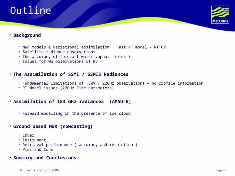
Outline

• Background

• NWP models & variational assimilation . Fast RT model – RTTOV.• Satellite radiance observations• The accuracy of forecast water vapour fields ?• Issues for MW observations of WV

• The Assimilation of SSMI / SSMIS Radiances

• Fundamental limitations of TCWV / 22GHz observations – no profile information• RT Model issues (22GHz line parameters)

• Assimilation of 183 GHz radiances (AMSU-B)

• Forward modelling in the presence of ice cloud

• Ground based MWR (nowcasting)

• 1DVar• Instrument• Retrieval performance ( accuracy and resolution )• Pros and Cons

• Summary and Conclusions


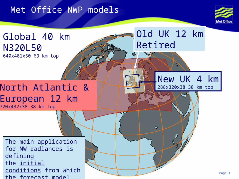
Met Office NWP models

Global 40 kmN320L50640x481x50 63 km top

North Atlantic & European 12 km720x432x38 38 km top

Old UK 12 kmRetired

New UK 4 km288x320x38 38 km top

The main applicationfor MW radiances is definingthe initial conditions from which the forecast model runs


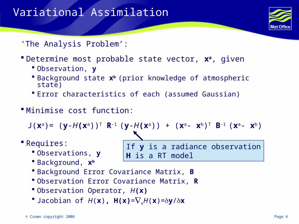
Variational Assimilation

‘The Analysis Problem’:

Determine most probable state vector, xa, given Observation, y Background state xb (prior knowledge of atmospheric state) Error characteristics of each (assumed Gaussian)

Minimise cost function:

J(xa)= (y-H(xa))T R-1 (y-H(xa)) + (xa- xb)T B-1 (xa- xb)

Requires: Observations, y Background, xb

Background Error Covariance Matrix, B Observation Error Covariance Matrix, R Observation Operator, H(x) Jacobian of H(x), H(x)=xH(x)=y/x

If y is a radiance observationH is a RT model


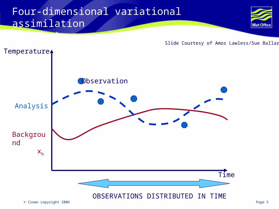
Four-dimensional variational assimilation(4D-Var)

Observation

Time

Temperature

Background xb

Analysis

Slide Courtesy of Amos Lawless/Sue Ballard

OBSERVATIONS DISTRIBUTED IN TIME


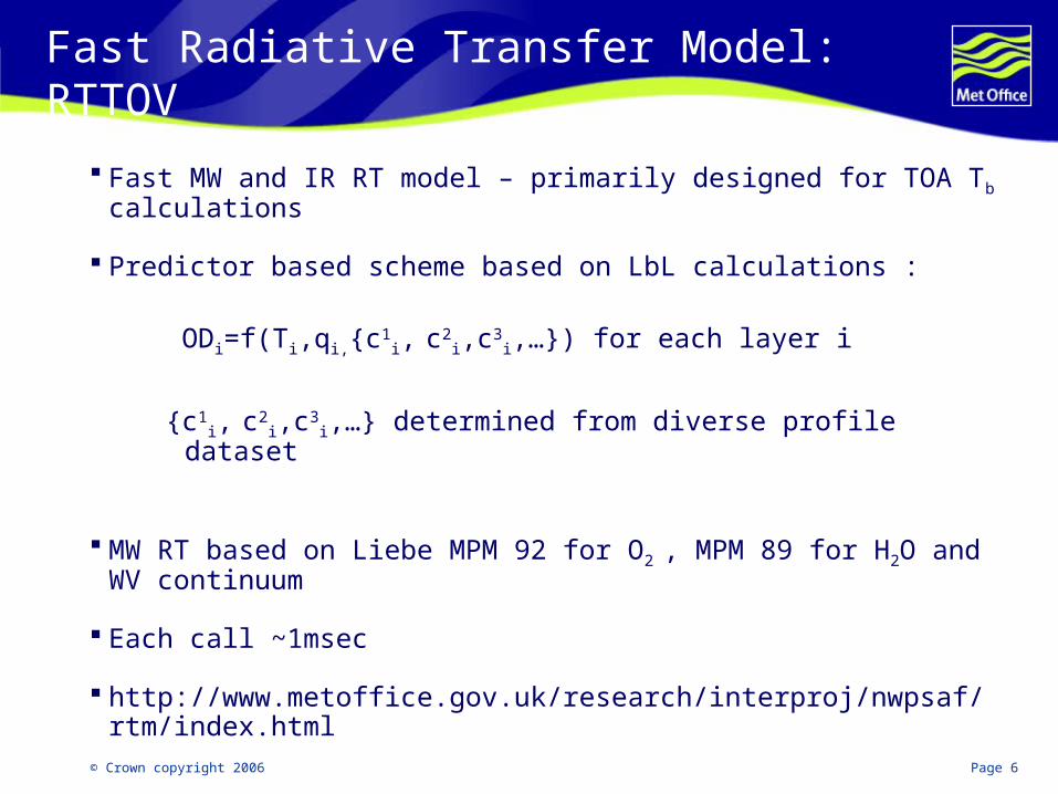
Fast Radiative Transfer Model: RTTOV

Fast MW and IR RT model – primarily designed for TOA Tb

calculations

Predictor based scheme based on LbL calculations :

ODi=f(Ti,qi,{c1i, c2

i,c3i,…}) for each layer i

{c1i, c2

i,c3i,…} determined from diverse profile dataset

MW RT based on Liebe MPM 92 for O2 , MPM 89 for H2O and WV continuum

Each call ~1msec

http://www.metoffice.gov.uk/research/interproj/nwpsaf/rtm/index.html


N

N15

N16

N18

N

AQUA

F13

N

F16

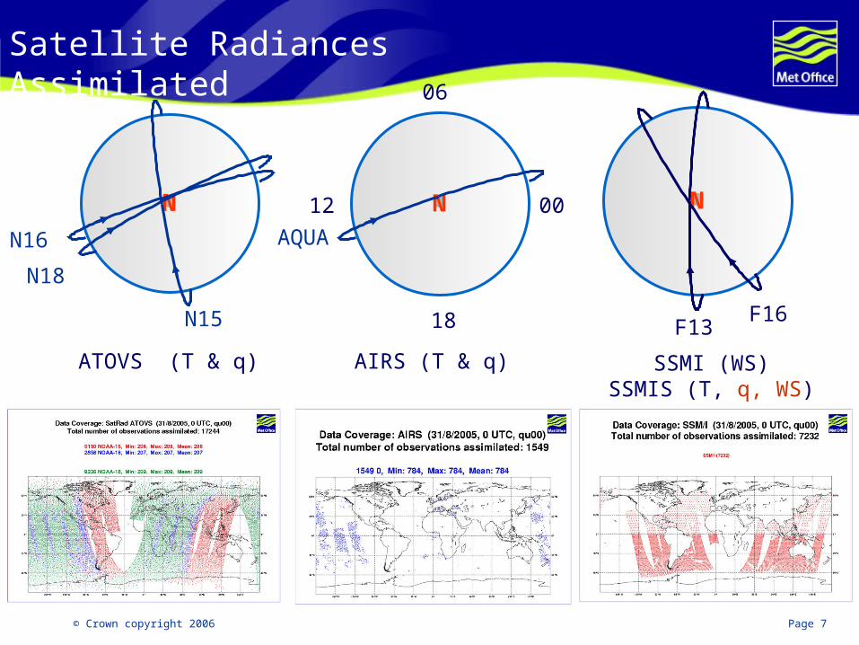
ATOVS (T & q) AIRS (T & q) SSMI (WS)SSMIS (T, q, WS)

Satellite Radiances Assimilated06

12

18

00


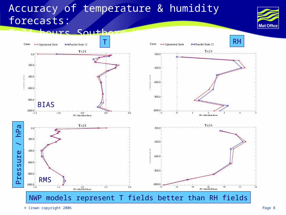
Accuracy of temperature & humidity forecasts:T+24 hours Southern Hemisphere

T RH

BIAS

RMS

NWP models represent T fields better than RH fields

Pre

ssur

e /

hPa


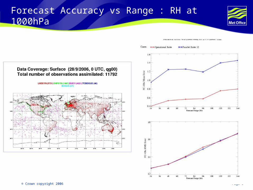
Forecast Accuracy vs Range : RH at 1000hPa


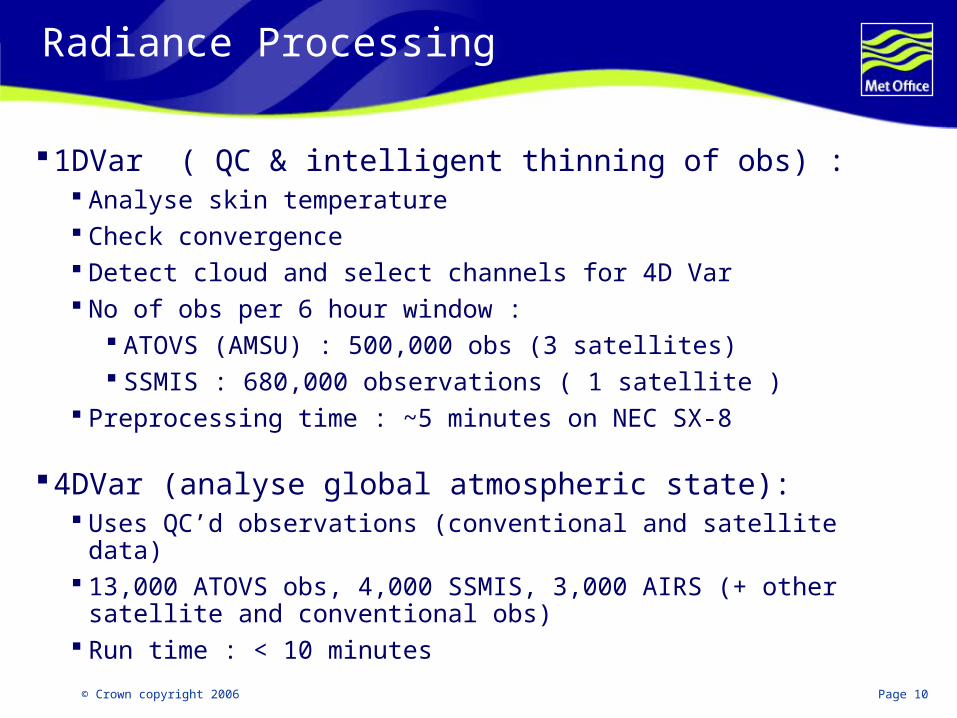
Radiance Processing

1DVar ( QC & intelligent thinning of obs) : Analyse skin temperature Check convergence Detect cloud and select channels for 4D Var No of obs per 6 hour window :

ATOVS (AMSU) : 500,000 obs (3 satellites) SSMIS : 680,000 observations ( 1 satellite )

Preprocessing time : ~5 minutes on NEC SX-8

4DVar (analyse global atmospheric state): Uses QC’d observations (conventional and satellite data) 13,000 ATOVS obs, 4,000 SSMIS, 3,000 AIRS (+ other satellite and

conventional obs) Run time : < 10 minutes


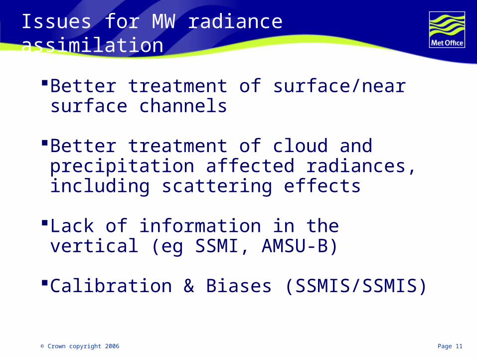
Issues for MW radiance assimilation

Better treatment of surface/near surface channels

Better treatment of cloud and precipitation affected radiances, including scattering effects

Lack of information in the vertical (eg SSMI, AMSU-B)

Calibration & Biases (SSMIS/SSMIS)

SSMI & SSMIS


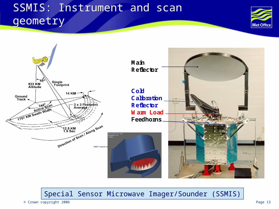
SSMIS: Instrument and scan geometrySSMIS: Instrument and scan geometry

MainReflector

ColdCalibrationReflectorWarm LoadFeedhorns

Special Sensor Microwave Imager/Sounder (SSMIS)


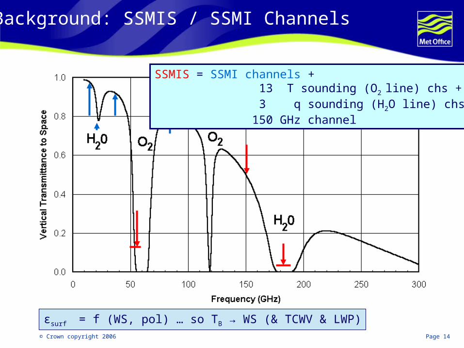
Background: SSMIS / SSMI Channels

SSMIS = SSMI channels + 13 T sounding (O2 line) chs + 3 q sounding (H2O line) chs + 150 GHz channel

εsurf = f (WS, pol) … so TB → WS (& TCWV & LWP)


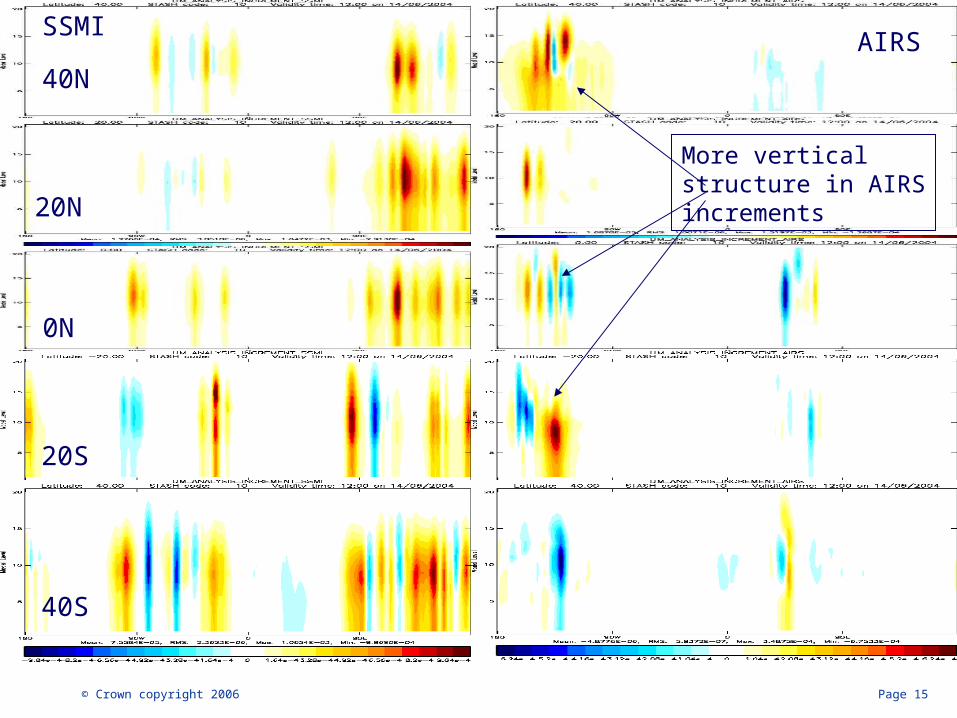
SSMI

40N

20N

0N

20S

40S

AIRS

More vertical structure in AIRSincrements


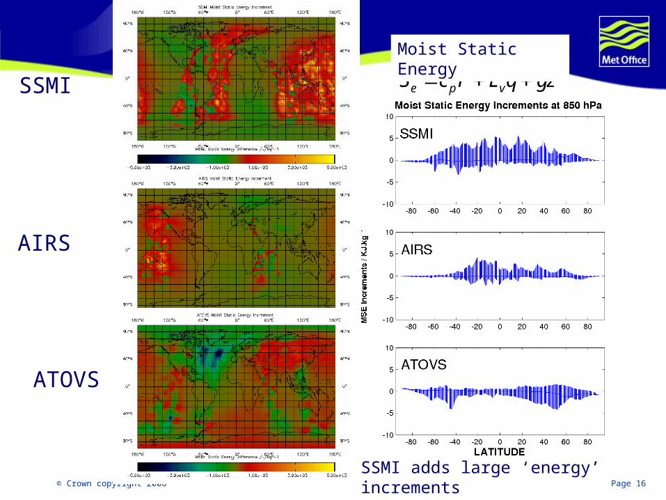
e p vS c T L q gz Moist Static Energy

SSMI

AIRS

ATOVS

SSMI adds large ‘energy’ increments


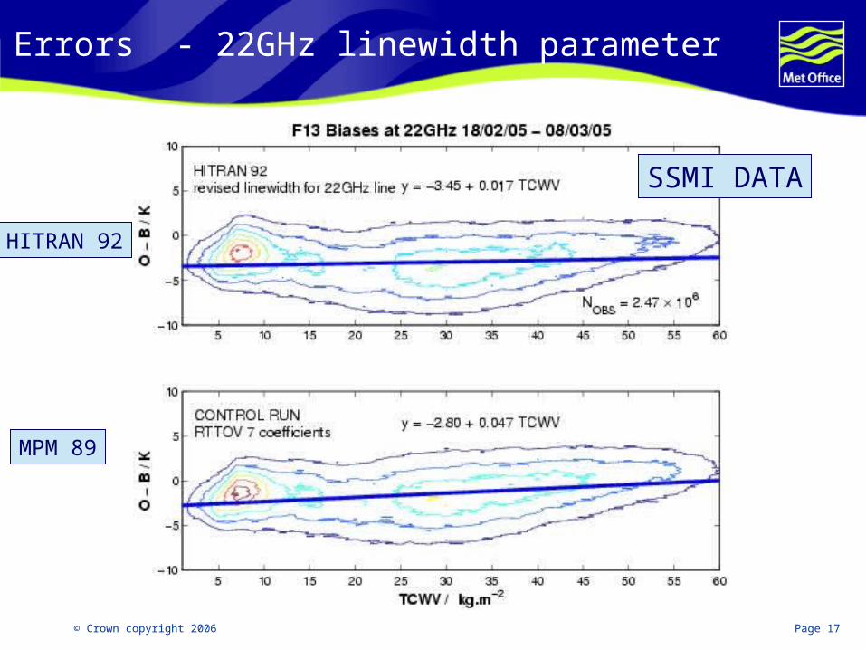
RT Errors - 22GHz linewidth parameter

SSMI DATA

MPM 89

HITRAN 92

Cloud Affected RadiancesScattering at 183 GHz


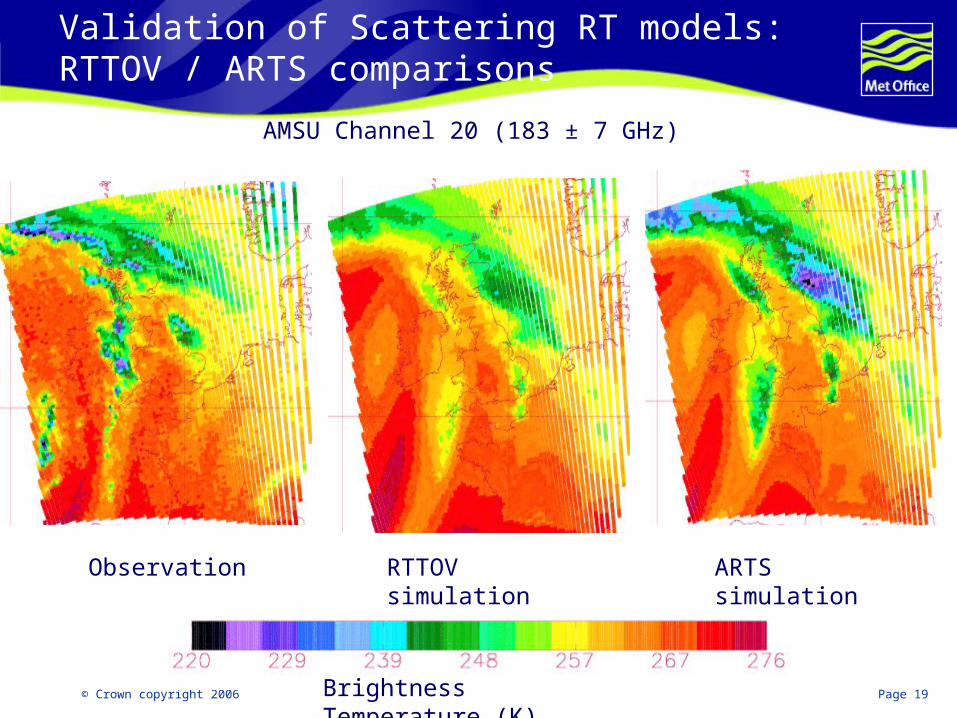
Validation of Scattering RT models:RTTOV / ARTS comparisons

AMSU Channel 20 (183 ± 7 GHz)

Observation ARTS simulationRTTOV simulation

Brightness Temperature (K)


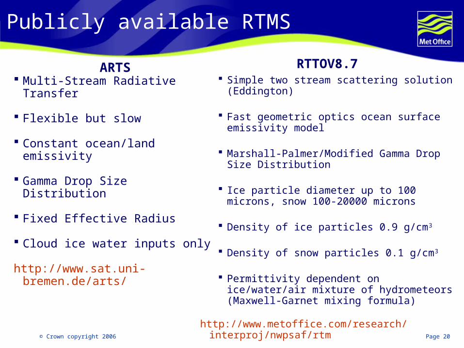
Publicly available RTMS

RTTOV8.7 Simple two stream scattering solution (Eddington)

Fast geometric optics ocean surface emissivity model

Marshall-Palmer/Modified Gamma Drop Size Distribution

Ice particle diameter up to 100 microns, snow 100-20000 microns

Density of ice particles 0.9 g/cm3

Density of snow particles 0.1 g/cm3

Permittivity dependent on ice/water/air mixture of hydrometeors (Maxwell-Garnet mixing formula)

http://www.metoffice.com/research/interproj/nwpsaf/rtm

ARTS Multi-Stream Radiative Transfer

Flexible but slow

Constant ocean/land emissivity

Gamma Drop Size Distribution

Fixed Effective Radius

Cloud ice water inputs only

http://www.sat.uni-bremen.de/arts/


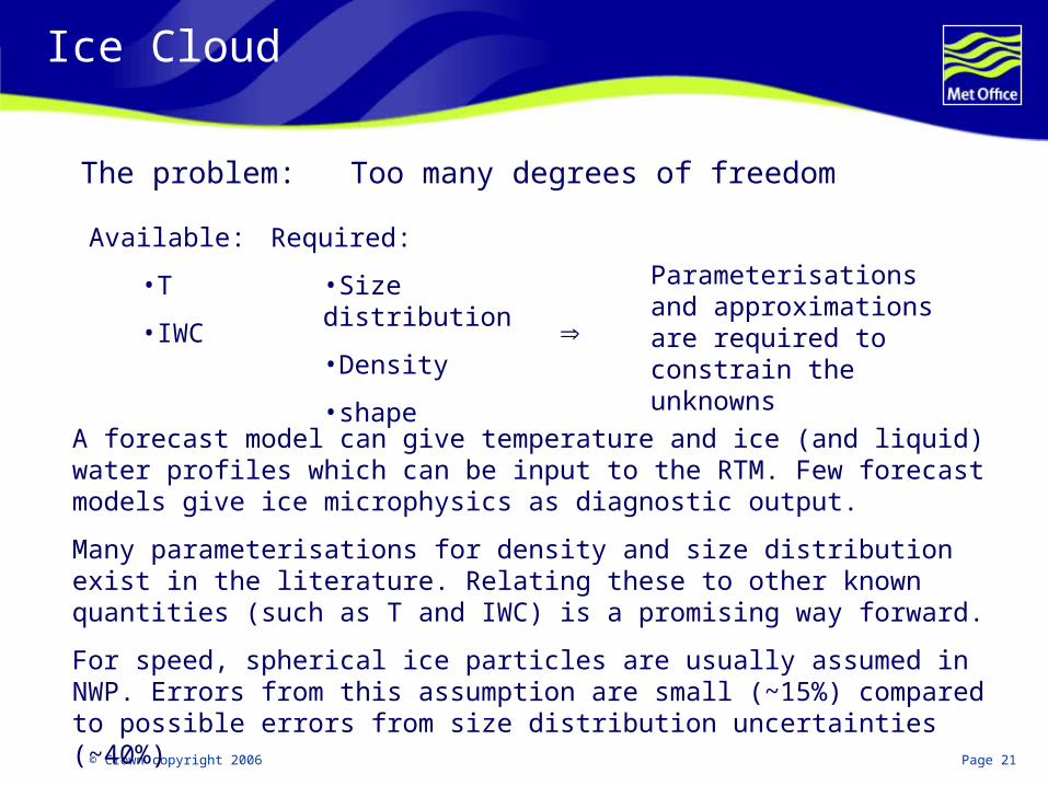
Ice Cloud

The problem: Too many degrees of freedom

Available:

•T

•IWC

Required:

•Size distribution

•Density

•shape

Parameterisations and approximations are required to constrain the unknowns

A forecast model can give temperature and ice (and liquid) water profiles which can be input to the RTM. Few forecast models give ice microphysics as diagnostic output.

Many parameterisations for density and size distribution exist in the literature. Relating these to other known quantities (such as T and IWC) is a promising way forward.

For speed, spherical ice particles are usually assumed in NWP. Errors from this assumption are small (~15%) compared to possible errors from size distribution uncertainties (~40%)

Ground Based MW radiometry


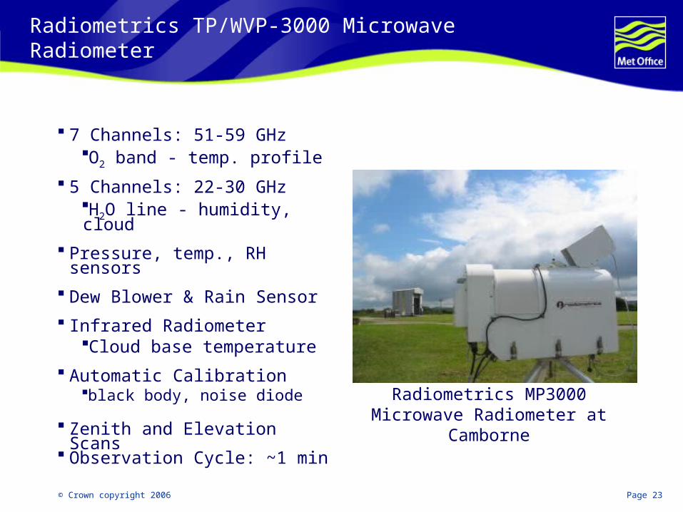
Radiometrics TP/WVP-3000 Microwave Radiometer

7 Channels: 51-59 GHzO2 band - temp. profile

5 Channels: 22-30 GHzH2O line - humidity, cloud

Pressure, temp., RH sensors

Dew Blower & Rain Sensor

Infrared RadiometerCloud base temperature

Automatic Calibrationblack body, noise diode

Zenith and Elevation Scans Observation Cycle: ~1 min

Radiometrics MP3000 Microwave Radiometer at Camborne


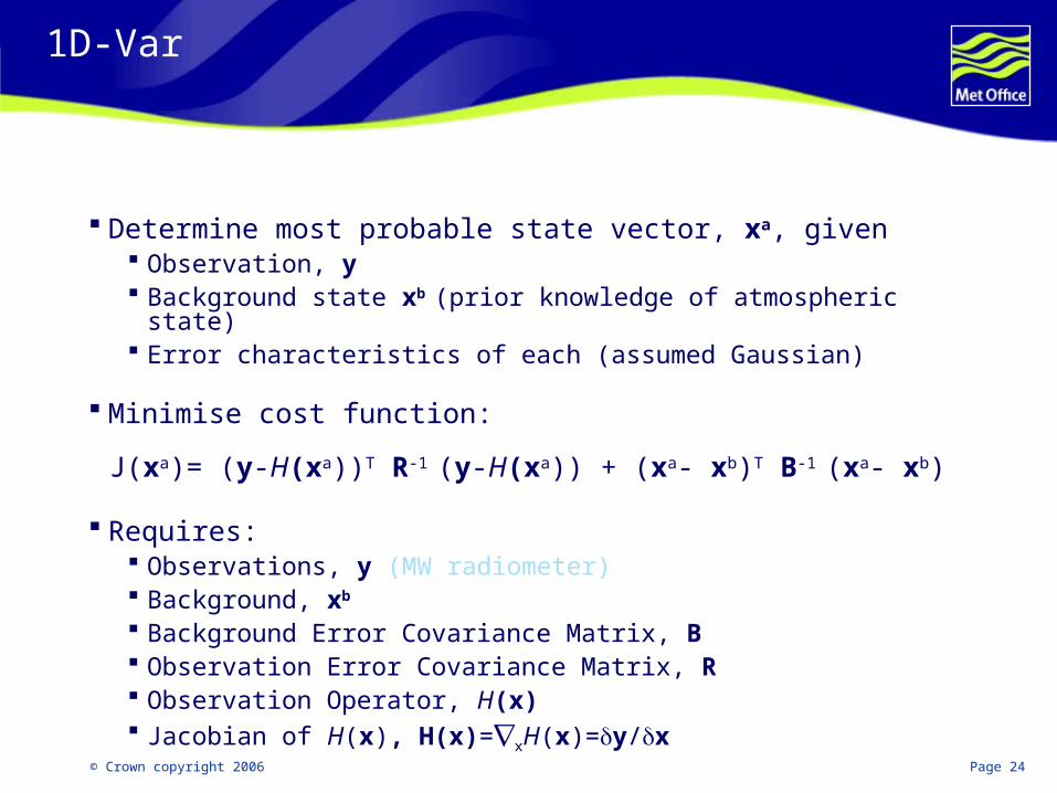
1D-Var

Determine most probable state vector, xa, given Observation, y Background state xb (prior knowledge of atmospheric state) Error characteristics of each (assumed Gaussian)

Minimise cost function:

J(xa)= (y-H(xa))T R-1 (y-H(xa)) + (xa- xb)T B-1 (xa- xb)

Requires: Observations, y (MW radiometer) Background, xb

Background Error Covariance Matrix, B Observation Error Covariance Matrix, R Observation Operator, H(x) Jacobian of H(x), H(x)=xH(x)=y/x


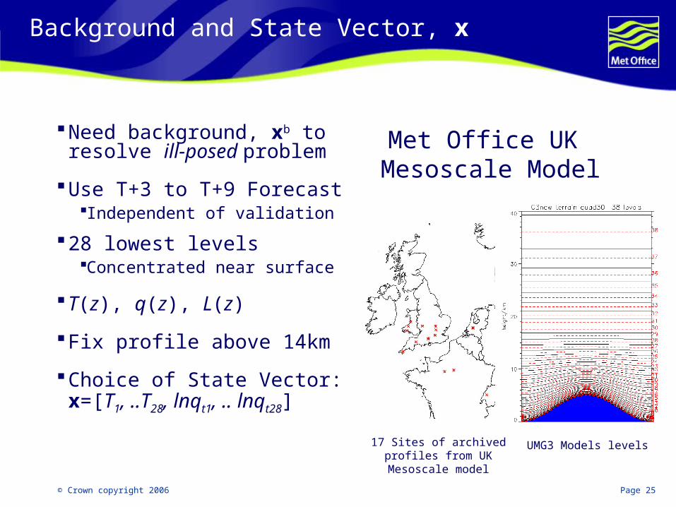
Background and State Vector, x

Need background, xb to resolve ill-posed problem

Use T+3 to T+9 ForecastIndependent of validation

28 lowest levelsConcentrated near surface

T(z), q(z), L(z)

Fix profile above 14km

Choice of State Vector: x=[T1, ..T28, lnqt1, .. lnqt28] 17 Sites of archived profiles

from UK Mesoscale modelUMG3 Models levels

Met Office UK Mesoscale Model


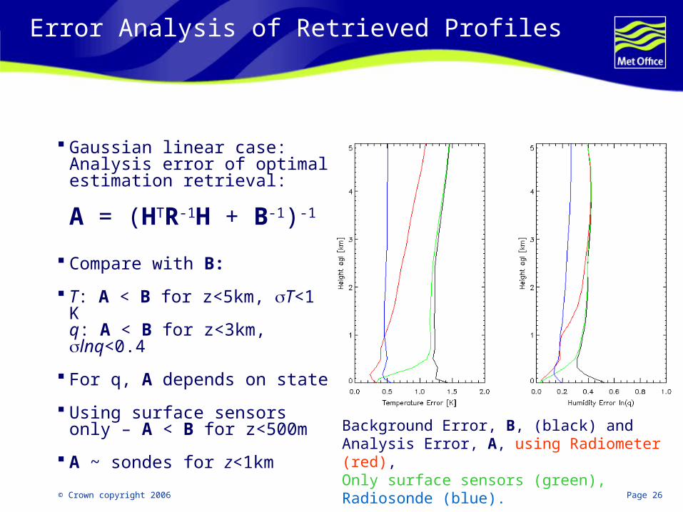
Error Analysis of Retrieved Profiles

Gaussian linear case:Analysis error of optimal estimation retrieval:

A = (HTR-1H + B-1)-1

Compare with B:

T: A < B for z<5km, T<1 Kq: A < B for z<3km, lnq<0.4

For q, A depends on state

Using surface sensors only – A < B for z<500m

A ~ sondes for z<1km

Background Error, B, (black) and Analysis Error, A, using Radiometer (red),Only surface sensors (green), Radiosonde (blue).


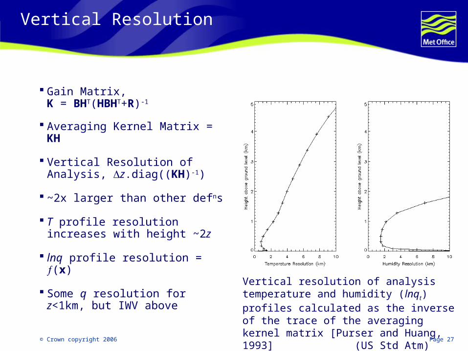
Vertical Resolution

Gain Matrix, K = BHT(HBHT+R)-1

Averaging Kernel Matrix = KH

Vertical Resolution of Analysis, z.diag((KH)-1)

~2x larger than other defns

T profile resolution increases with height ~2z

lnq profile resolution = (x)

Some q resolution for z<1km, but IWV above

Vertical resolution of analysis temperature and humidity (lnqt) profiles calculated as the inverse of the trace of the averaging kernel matrix [Purser and Huang, 1993] (US Std Atm)


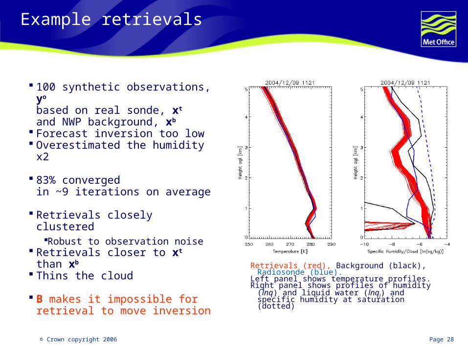
Example retrievals

100 synthetic observations, yo

based on real sonde, xt and NWP background, xb

Forecast inversion too low Overestimated the humidity x2

83% converged in ~9 iterations on average

Retrievals closely clusteredRobust to observation noise

Retrievals closer to xt than xb

Thins the cloud

B makes it impossible for retrieval to move inversion

Retrievals (red), Background (black), Radiosonde (blue).

Left panel shows temperature profiles. Right panel shows profiles of humidity (lnq)

and liquid water (lnql) and specific humidity at saturation (dotted)


Ground based MW radiometry: Conclusions

Pros Optimal method to integrate observations with background Provides estimate of error in retrieval Shows impact from MWR below ~4km – most <1km

Cons Fundamentally poor vertical resolution of passive profilers Convergence problems for very non-linear problems Difficult when background is wrong (shifting patterns)

Future Work Add ceilometer cloud base/cloud radar tops/GPS IWV to y Integrate with Wind Profiler SNR – e.g. Boundary Layer top How to exploit high time resolution? 4D-VAR? Variability?


Summary & Conclusions

MW radiances are an important component of operational NWP systems, it is now normal to assimilate these directly as radiances, rather than using retrievals

Variational assimilation (1d, 3d or 4d) is an optimal way of combining background and observational information to define an atmospheric state

Fast RT models are important in achieving this

Challenges presented by MW radiance measurements include : dealing with cloud and precipitation, limited vertical resolution, biases (eg RT biases)

Ground based MWR is being assessed for nowcasting and assimilation applications. Column water estimates are accurate , but vertical resolution is poor (~1km for q)

Page 1© Crown copyright 2006 The Analysis of Water Vapour in Met Office NWP Models Bill Bell (SSMI,...

Documents

Transcript of Page 1© Crown copyright 2006 The Analysis of Water Vapour in Met Office NWP Models Bill Bell (SSMI,...