Optimal Highway Traffic Control using a

Velocity-Cell Transmission Model

Alessandro Castagnotto

Nicholas Wong

Outline

Problem Description and Motivation

Cell Transmission Model

Godunov Flux function

Cell Transmission Model for Velocity

Optimal Control Problem

Flux as a minimization problem

Conclusions and Outlook

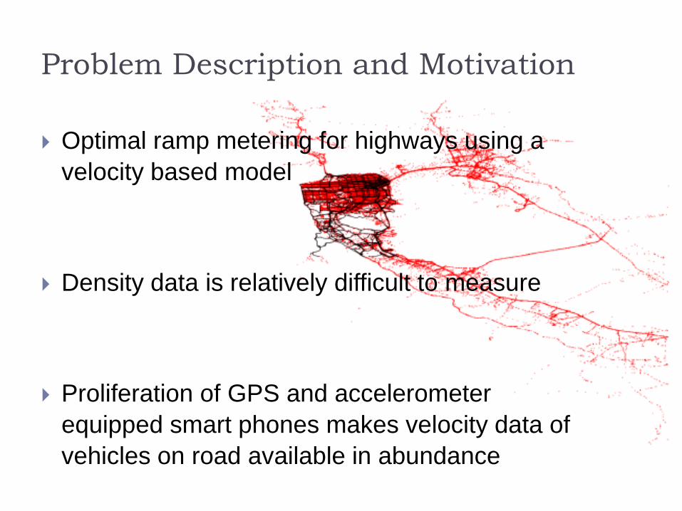
Problem Description and Motivation

Optimal ramp metering for highways using a

velocity based model

Density data is relatively difficult to measure

Proliferation of GPS and accelerometer

equipped smart phones makes velocity data of

vehicles on road available in abundance

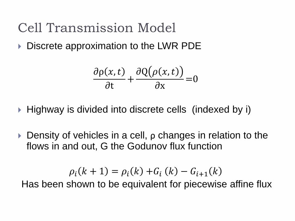
Cell Transmission Model

Discrete approximation to the LWR PDE

∂ρ 𝑥, 𝑡

∂t+∂Q 𝜌 𝑥, 𝑡

∂x=0

Highway is divided into discrete cells (indexed by i)

Density of vehicles in a cell, ρ changes in relation to the flows in and out, G the Godunov flux function

𝜌𝑖 𝑘 + 1 = 𝜌𝑖 𝑘 +𝐺𝑖 𝑘 − 𝐺𝑖+1 𝑘

Has been shown to be equivalent for piecewise affine flux

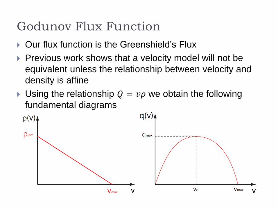
Godunov Flux Function

Our flux function is the Greenshield’s Flux

Previous work shows that a velocity model will not be

equivalent unless the relationship between velocity and

density is affine

Using the relationship 𝑄 = 𝑣𝜌 we obtain the following

fundamental diagrams

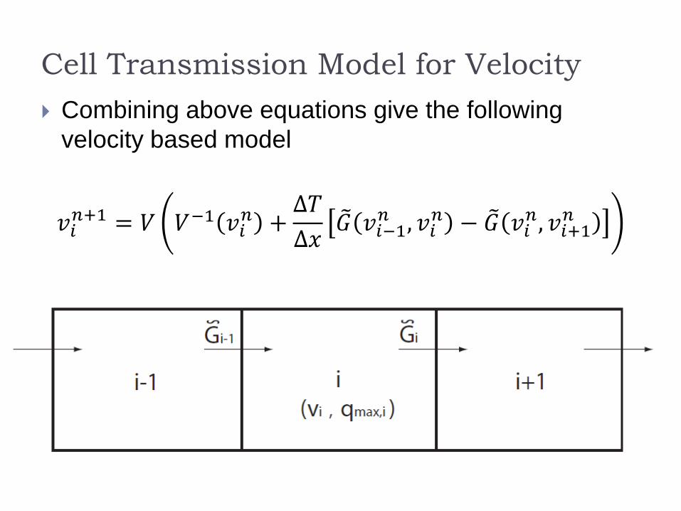
Cell Transmission Model for Velocity

Combining above equations give the following

velocity based model

𝑣𝑖𝑛+1 = 𝑉 𝑉−1 𝑣𝑖

𝑛 +∆𝑇

∆𝑥𝐺 𝑣𝑖−1

𝑛 , 𝑣𝑖𝑛 − 𝐺 𝑣𝑖

𝑛, 𝑣𝑖+1𝑛

Godunov Flux

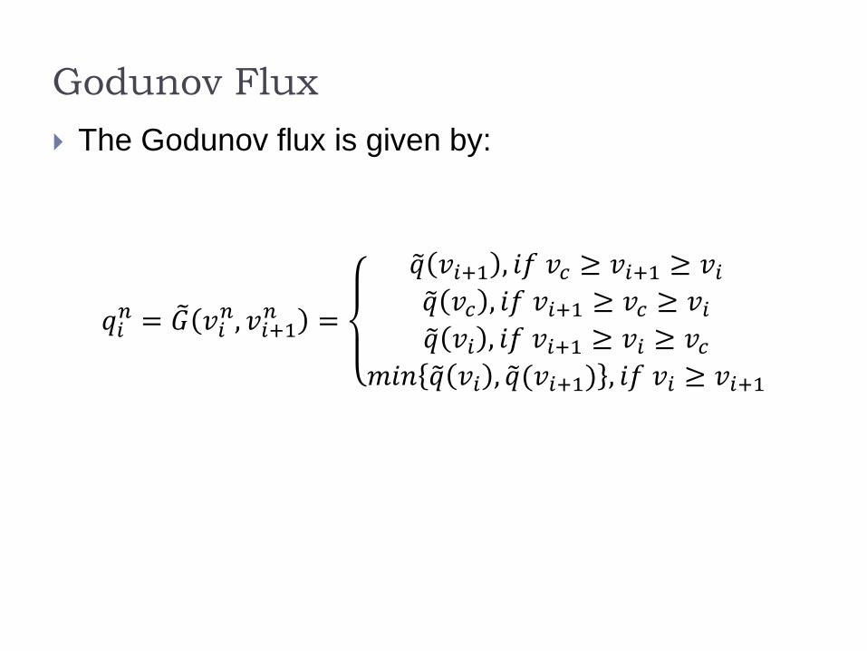
The Godunov flux is given by:

𝑞𝑖𝑛 = 𝐺 𝑣𝑖

𝑛, 𝑣𝑖+1𝑛 =

𝑞 𝑣𝑖+1 , 𝑖𝑓 𝑣𝑐 ≥ 𝑣𝑖+1 ≥ 𝑣𝑖𝑞 𝑣𝑐 , 𝑖𝑓 𝑣𝑖+1 ≥ 𝑣𝑐 ≥ 𝑣𝑖𝑞 𝑣𝑖 , 𝑖𝑓 𝑣𝑖+1 ≥ 𝑣𝑖 ≥ 𝑣𝑐

𝑚𝑖𝑛 𝑞 𝑣𝑖 , 𝑞 (𝑣𝑖+1) , 𝑖𝑓 𝑣𝑖 ≥ 𝑣𝑖+1

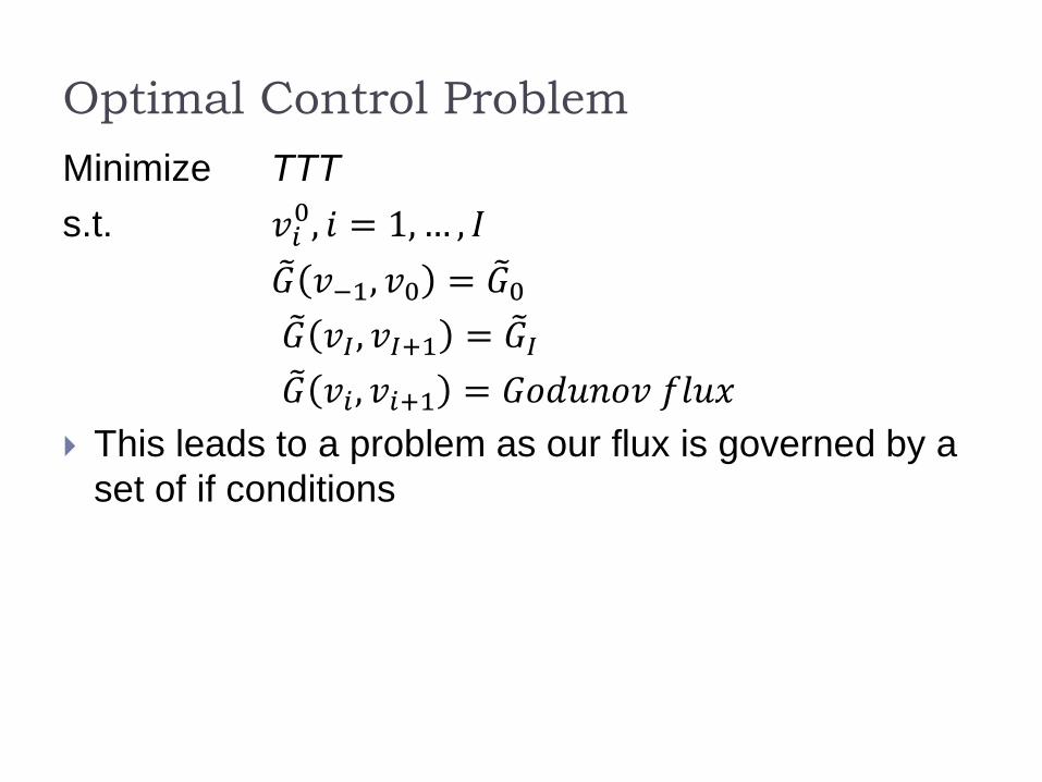
Optimal Control Problem

Minimize TTT

s.t. 𝑣𝑖0, 𝑖 = 1, … , 𝐼

𝐺 𝑣−1, 𝑣0 = 𝐺 0

𝐺 𝑣𝐼, 𝑣𝐼+1 = 𝐺 𝐼

𝐺 𝑣𝑖 , 𝑣𝑖+1 = 𝐺𝑜𝑑𝑢𝑛𝑜𝑣 𝑓𝑙𝑢𝑥

This leads to a problem as our flux is governed by a

set of if conditions

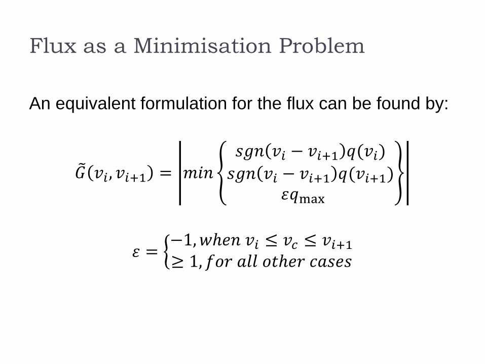
Flux as a Minimisation Problem

An equivalent formulation for the flux can be found by:

𝐺 𝑣𝑖 , 𝑣𝑖+1 = 𝑚𝑖𝑛𝑠𝑔𝑛 𝑣𝑖 − 𝑣𝑖+1 𝑞(𝑣𝑖)

𝑠𝑔𝑛 𝑣𝑖 − 𝑣𝑖+1 𝑞(𝑣𝑖+1)𝜀𝑞max

𝜀 = −1,𝑤ℎ𝑒𝑛 𝑣𝑖 ≤ 𝑣𝑐 ≤ 𝑣𝑖+1≥ 1, 𝑓𝑜𝑟 𝑎𝑙𝑙 𝑜𝑡ℎ𝑒𝑟 𝑐𝑎𝑠𝑒𝑠

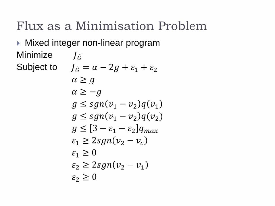
Flux as a Minimisation Problem

Mixed integer non-linear program

Minimize 𝐽𝐺

Subject to 𝐽𝐺 = 𝛼 − 2𝑔 + 𝜀1 + 𝜀2

𝛼 ≥ 𝑔

𝛼 ≥ −𝑔

𝑔 ≤ 𝑠𝑔𝑛 𝑣1 − 𝑣2 𝑞 𝑣1

𝑔 ≤ 𝑠𝑔𝑛 𝑣1 − 𝑣2 𝑞(𝑣2)

𝑔 ≤ 3 − 𝜀1 − 𝜀2 𝑞𝑚𝑎𝑥

𝜀1 ≥ 2𝑠𝑔𝑛 𝑣2 − 𝑣𝑐

𝜀1 ≥ 0

𝜀2 ≥ 2𝑠𝑔𝑛 𝑣2 − 𝑣1

𝜀2 ≥ 0

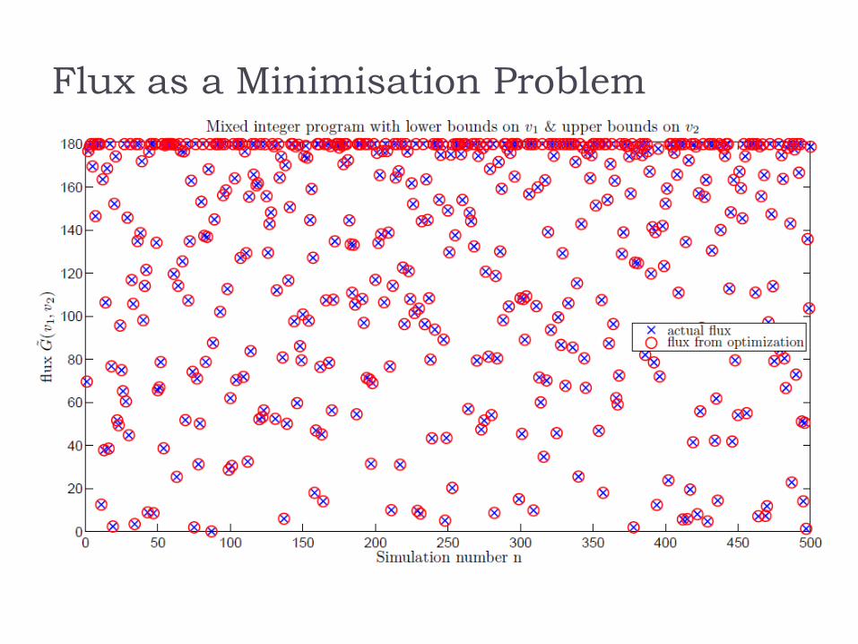
Flux as a Minimisation Problem

Conclusions and Outlook

We are able to correctly determine flux despite non

linearities in the problem

Slack variables affect our cost

For control purposes the cost formulation needs to

be tweaked or to reformulate the problem such that

slack variables are not required (such as Big-M

formulation)

Infeasibilities with solvers when using system

dynamics

Additional Material

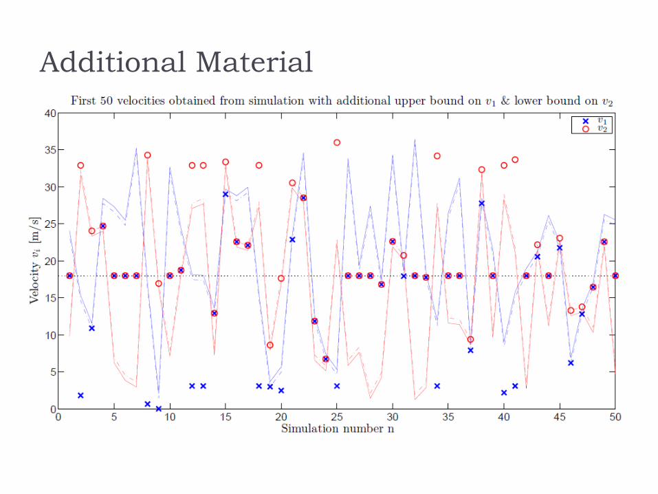
Additional Material

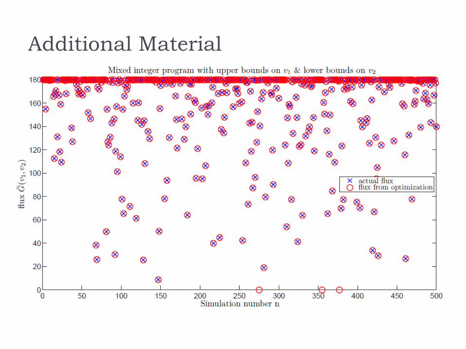
Additional Material

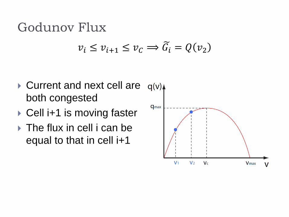
Godunov Flux

𝑣𝑖 ≤ 𝑣𝑖+1 ≤ 𝑣𝐶 ⟹ 𝐺𝑖 = 𝑄 𝑣2

Current and next cell are

both congested

Cell i+1 is moving faster

The flux in cell i can be

equal to that in cell i+1

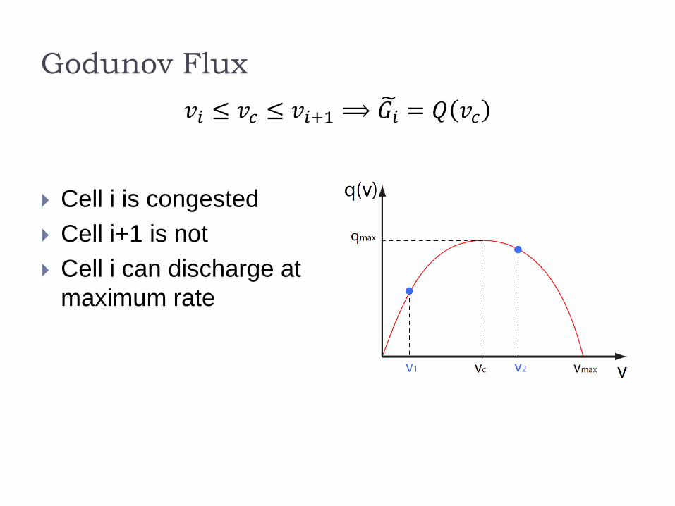
Godunov Flux

𝑣𝑖 ≤ 𝑣𝑐 ≤ 𝑣𝑖+1 ⟹ 𝐺𝑖 = 𝑄 𝑣𝑐

Cell i is congested

Cell i+1 is not

Cell i can discharge at

maximum rate

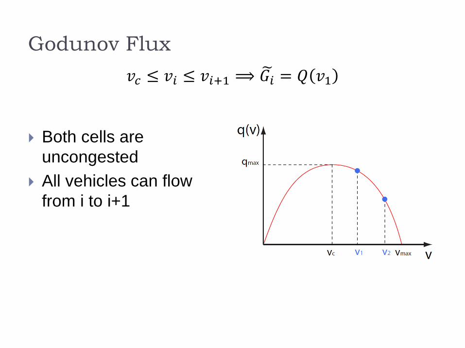
Godunov Flux

𝑣𝑐 ≤ 𝑣𝑖 ≤ 𝑣𝑖+1 ⟹ 𝐺𝑖 = 𝑄 𝑣1

Both cells are

uncongested

All vehicles can flow

from i to i+1

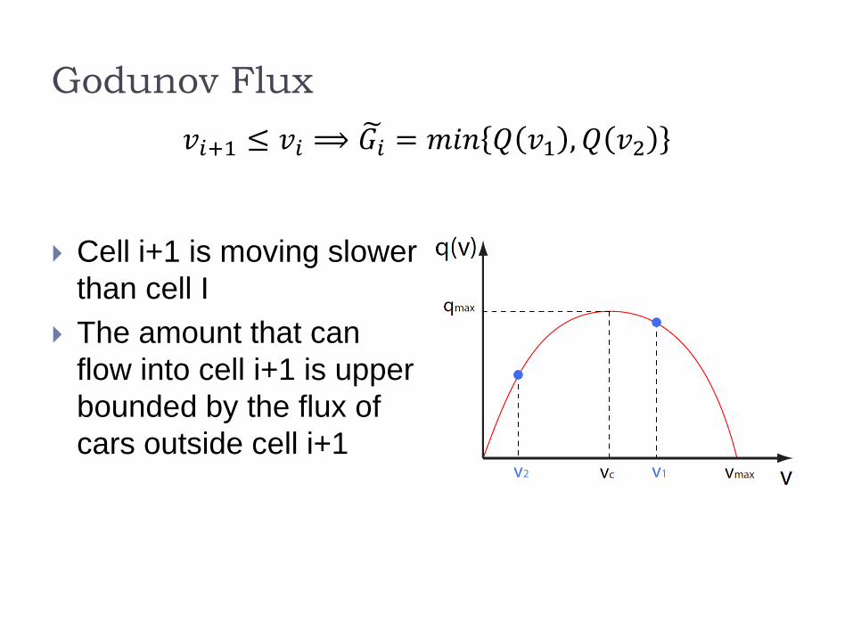
Godunov Flux

𝑣𝑖+1 ≤ 𝑣𝑖 ⟹ 𝐺𝑖 = 𝑚𝑖𝑛 𝑄 𝑣1 , 𝑄 𝑣2

Cell i+1 is moving slower

than cell I

The amount that can

flow into cell i+1 is upper

bounded by the flux of

cars outside cell i+1

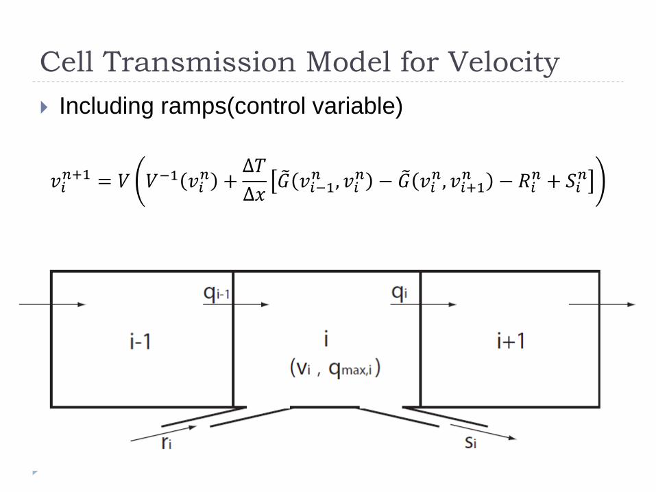
Cell Transmission Model for Velocity

Including ramps(control variable)

𝑣𝑖𝑛+1 = 𝑉 𝑉−1 𝑣𝑖

𝑛 +∆𝑇

∆𝑥𝐺 𝑣𝑖−1

𝑛 , 𝑣𝑖𝑛 − 𝐺 𝑣𝑖

𝑛, 𝑣𝑖+1𝑛 − 𝑅𝑖

𝑛 + 𝑆𝑖𝑛