
Ιούλιος 2014 NETMODE Network Management & Optimal Design Lab
Optimal collapse simulator for three-dimensionalstructures
Ferran Vidal CodinaE.T.S. Enginyers de Camins, UPC Barcelona Tech
C/ Jordi Girona 1, 08034 BARCELONA
February 16, 2011
Abstract
In this project limit analysis for 3D structures is studied. The goal is toobtain for a certain structure the load factor λ that applied to the externalloads induces collapse to the structure. The static theorem of limit analysisis the theoretical basis for the Structural Collapse Simulator (SCS), that isfinding a stress distribution in equilibrium that does not violate yield crite-ria anywhere. This theorem is employed combined with linear programmingtechniques. Thereby a tutorial on LP problems is presented first. Then abrief summary of the progresses in study of limit analysis for structures isoffered, being a useful introduction for understanding the very nature of SCSfunctioning. Moreover, limit analysis is developed and written as a LP prob-lem, which consists of the maximization of the collapse load factor subject toequilibrium and yield criteria.
Two major contributions are presented for finding the collapse load. Firstly,the yield curve of standard 2D beam cross sections is adaptively approxi-mated with inscribed and circumscribed polygons that yield to lower andupper bounds of λ respectively. Secondly, an interesting approach for ac-counting with uniform distributed loads is shown, producing bounding of theload factor. Combining these two techniques the bound gap can be reducedarbitrarily, observing convergence of the upper and the lower bounds to theexact load factor. A tutorial for using SCS and computing structures is pro-vided, and numerical examples are thoroughly studied in order to illustratethe functioning of the program and the limits of the method. Finally, re-cent developments and future branches of research are detailed in order towiden the applicability range of SCS, the most important being the adaptiveapproximation of the yield surface for 3D beams.
1
CONTENTS
Contents
1 Motivation and acknowledgements 7
2 Optimization and LP, Duality and Lagrange Multipliers 82.1 Optimization Problems . . . . . . . . . . . . . . . . . . . . . . . . . . 82.2 Lagrange dual function and duality . . . . . . . . . . . . . . . . . . . 9
2.2.1 Lagrangian . . . . . . . . . . . . . . . . . . . . . . . . . . . . 92.2.2 Lagrange dual function . . . . . . . . . . . . . . . . . . . . . . 92.2.3 Lower bounds on optimal value . . . . . . . . . . . . . . . . . 92.2.4 The Lagrange dual problem . . . . . . . . . . . . . . . . . . . 102.2.5 The weak duality . . . . . . . . . . . . . . . . . . . . . . . . . 102.2.6 The strong duality . . . . . . . . . . . . . . . . . . . . . . . . 11
2.3 Linear optimization problems . . . . . . . . . . . . . . . . . . . . . . 112.3.1 LP in standard form, its dual and extended dual theorem . . . 112.3.2 LP in general form, lagrangian and duality . . . . . . . . . . . 12
3 Evolution in limit analysis techniques 13
4 Limit state analysis as a LP problem 174.1 Equilibrium . . . . . . . . . . . . . . . . . . . . . . . . . . . . . . . . 18
4.1.1 Local equilibrium . . . . . . . . . . . . . . . . . . . . . . . . . 194.1.2 Rotation . . . . . . . . . . . . . . . . . . . . . . . . . . . . . . 194.1.3 The 2D Structure . . . . . . . . . . . . . . . . . . . . . . . . . 204.1.4 Equilibrium for trusses . . . . . . . . . . . . . . . . . . . . . . 214.1.5 Global equilibrium . . . . . . . . . . . . . . . . . . . . . . . . 21
4.2 Yield criteria . . . . . . . . . . . . . . . . . . . . . . . . . . . . . . . 224.2.1 Class type . . . . . . . . . . . . . . . . . . . . . . . . . . . . . 234.2.2 Yield function definition . . . . . . . . . . . . . . . . . . . . . 244.2.3 Yield curve linearization . . . . . . . . . . . . . . . . . . . . . 254.2.4 Yield criteria as a LP problem . . . . . . . . . . . . . . . . . . 274.2.5 Yield criteria for trusses . . . . . . . . . . . . . . . . . . . . . 30
4.3 Inclusion of Uniform Distributed Loads . . . . . . . . . . . . . . . . . 314.3.1 Combination of yield and UDL bounding . . . . . . . . . . . . 34
4.4 The LP problem . . . . . . . . . . . . . . . . . . . . . . . . . . . . . 344.4.1 Upper Bound . . . . . . . . . . . . . . . . . . . . . . . . . . . 354.4.2 Lower Bound . . . . . . . . . . . . . . . . . . . . . . . . . . . 364.4.3 Problem normalization . . . . . . . . . . . . . . . . . . . . . . 374.4.4 Evaluation of the bound gap . . . . . . . . . . . . . . . . . . . 37
5 Use of Structural Collapse Simulator 385.1 Data input . . . . . . . . . . . . . . . . . . . . . . . . . . . . . . . . . 39
5.1.1 Logicals for structure characterization . . . . . . . . . . . . . . 395.1.2 Nodal and Connectivity matrices . . . . . . . . . . . . . . . . 39
Ferran Vidal Codina 2
CONTENTS
5.1.3 External Load matrices . . . . . . . . . . . . . . . . . . . . . . 405.1.4 Geometric Restrictions matrix . . . . . . . . . . . . . . . . . . 405.1.5 Example of data input . . . . . . . . . . . . . . . . . . . . . . 41
5.2 Data processing . . . . . . . . . . . . . . . . . . . . . . . . . . . . . . 435.2.1 Initialization of variables . . . . . . . . . . . . . . . . . . . . . 435.2.2 Setting approximation for yield criteria . . . . . . . . . . . . . 435.2.3 Dimensional check . . . . . . . . . . . . . . . . . . . . . . . . 44
5.3 Creation of matrices . . . . . . . . . . . . . . . . . . . . . . . . . . . 445.3.1 Equilibrium matrices . . . . . . . . . . . . . . . . . . . . . . . 455.3.2 Yield criteria matrices . . . . . . . . . . . . . . . . . . . . . . 45
5.4 LP Solver . . . . . . . . . . . . . . . . . . . . . . . . . . . . . . . . . 475.5 Postprocessing . . . . . . . . . . . . . . . . . . . . . . . . . . . . . . . 48
5.5.1 Gap Evaluation . . . . . . . . . . . . . . . . . . . . . . . . . . 485.5.2 Plotting plastic hinges and displacement rates . . . . . . . . . 485.5.3 Plotting elements failure . . . . . . . . . . . . . . . . . . . . . 495.5.4 Plotting bending moment diagram . . . . . . . . . . . . . . . 495.5.5 Time of computation . . . . . . . . . . . . . . . . . . . . . . . 505.5.6 Example of postprocessing . . . . . . . . . . . . . . . . . . . . 50
5.6 Cross Section Library . . . . . . . . . . . . . . . . . . . . . . . . . . . 515.6.1 I/H-shaped . . . . . . . . . . . . . . . . . . . . . . . . . . . . 525.6.2 C4 Sections . . . . . . . . . . . . . . . . . . . . . . . . . . . . 53
5.7 Utility of SCS . . . . . . . . . . . . . . . . . . . . . . . . . . . . . . . 535.7.1 Linear analysis . . . . . . . . . . . . . . . . . . . . . . . . . . 535.7.2 Nonlinear analysis . . . . . . . . . . . . . . . . . . . . . . . . 545.7.3 SCS . . . . . . . . . . . . . . . . . . . . . . . . . . . . . . . . 54
6 Numerical examples 546.1 Simply supported beam . . . . . . . . . . . . . . . . . . . . . . . . . 54
6.1.1 Simply supported beam with no subdivision . . . . . . . . . . 566.1.2 Simply supported beam with one subdivision . . . . . . . . . . 576.1.3 Simply supported beam with two subdivisions . . . . . . . . . 596.1.4 Simply supported beam with three subdivisions . . . . . . . . 59
6.2 Embedded frame with point load . . . . . . . . . . . . . . . . . . . . 626.3 Steel tower . . . . . . . . . . . . . . . . . . . . . . . . . . . . . . . . . 646.4 Model of a 2D three-storey building . . . . . . . . . . . . . . . . . . . 65
6.4.1 Frame with no span subdivision . . . . . . . . . . . . . . . . . 666.4.2 Frame with one span subdivision . . . . . . . . . . . . . . . . 676.4.3 Frame with two span subdivisions . . . . . . . . . . . . . . . . 686.4.4 Frame with manual subdivisions . . . . . . . . . . . . . . . . . 696.4.5 Study of convergence . . . . . . . . . . . . . . . . . . . . . . . 70
6.5 Model of a 3D two-storey building . . . . . . . . . . . . . . . . . . . . 73
7 Conclusions 74
Ferran Vidal Codina 3

CONTENTS
8 Future research 778.1 3D Frames yield criteria . . . . . . . . . . . . . . . . . . . . . . . . . 778.2 Cross Section Library . . . . . . . . . . . . . . . . . . . . . . . . . . . 788.3 LP solver . . . . . . . . . . . . . . . . . . . . . . . . . . . . . . . . . 788.4 Adaptivity . . . . . . . . . . . . . . . . . . . . . . . . . . . . . . . . . 78
Ferran Vidal Codina 4
LIST OF FIGURES
List of Figures
1 Generalized stresses in a 3D beam element . . . . . . . . . . . . . . . 182 Nodal forces and moments in a beam element . . . . . . . . . . . . . 183 I/H-shaped symmetric cross section . . . . . . . . . . . . . . . . . . . 244 Yield curve for IPE550 (red) and HEB300 (green) cross sections . . . . 255 Inscribed and circumscribed polygons of a IPE550 yield curve using
8/10 lines per node respectively . . . . . . . . . . . . . . . . . . . . . 266 Simplest linearization for a general yield surface . . . . . . . . . . . . 287 Moment diagram with secant and tangent approximation for a beam
with UDL . . . . . . . . . . . . . . . . . . . . . . . . . . . . . . . . . 328 Schematic representation for a basic triangular structure . . . . . . . 419 SCS output of PlotStructures function for the triangular frame . . . . 4210 SCS output of PlotHinges function for the triangular frame . . . . . . 5011 SCS output of PlotMoments function for the triangular frame . . . . 5112 Simply supported beam of length l: (a) Loading and reactions, (b)
Bending moment, (c) Shear stress . . . . . . . . . . . . . . . . . . . . 5513 Simply supported beam with no span subdivision . . . . . . . . . . . 5614 Plastic hinge detection by SCS for the simply supported beam with
no subdivision . . . . . . . . . . . . . . . . . . . . . . . . . . . . . . . 5715 Bending moment distribution for the simply supported beam with
one span subdivision . . . . . . . . . . . . . . . . . . . . . . . . . . . 5816 Plastic hinge detection by SCS for the simply supported beam with
one span subdivision . . . . . . . . . . . . . . . . . . . . . . . . . . . 5817 Bending moment distribution for the simply supported beam with
two span subdivisions . . . . . . . . . . . . . . . . . . . . . . . . . . . 5918 Bending moment distribution for the simply supported beam with
three span subdivisions . . . . . . . . . . . . . . . . . . . . . . . . . . 6019 Convergence for λ and ∆ versus the number of elements . . . . . . . 6120 Representation of the embedded frame with point load . . . . . . . . 6121 SCS detection of the plastic hinges to form the collapse mechanism . 6222 Schematic representation and 3D view of the steel tower . . . . . . . 6323 Collapse mechanism. In red elements that fail for traction and in blue
for compression . . . . . . . . . . . . . . . . . . . . . . . . . . . . . . 6424 Amplified deformed structure in blue. . . . . . . . . . . . . . . . . . . 6425 Representation of the three-storey frame . . . . . . . . . . . . . . . . 6526 Convergence of λ and ∆ versus the number of lines for the frame with
no span subdivision . . . . . . . . . . . . . . . . . . . . . . . . . . . . 6627 Convergence of λ and ∆ versus the number of lines for the frame with
one span subdivision . . . . . . . . . . . . . . . . . . . . . . . . . . . 6728 Convergence of λ and ∆ versus the number of lines for the frame with
two span subdivisions . . . . . . . . . . . . . . . . . . . . . . . . . . . 6829 SCS output for moment distribution for the frame with two span
subdivisions . . . . . . . . . . . . . . . . . . . . . . . . . . . . . . . . 69
Ferran Vidal Codina 5
LIST OF TABLES
30 Convergence of λ and ∆ versus the number of lines for the frame withan extra manual span subdivisions . . . . . . . . . . . . . . . . . . . 70
31 Plastic hinge detection by SCS for the frame with an extra manualsubdivision . . . . . . . . . . . . . . . . . . . . . . . . . . . . . . . . 71
32 Convergence of λ and ∆ versus the number of lines for the frame . . . 7233 Representation of the 3D two-storey frame . . . . . . . . . . . . . . . 7334 Convergence of λ and ∆ versus the number of subdivisions . . . . . . 7435 Plastic hinge detection by SCS for the 3D two-storey frame with three
subdivisions . . . . . . . . . . . . . . . . . . . . . . . . . . . . . . . . 7536 Yield surface for IPE360 cross section . . . . . . . . . . . . . . . . . . 77
List of Tables
1 Variable assignation depending on dimension and structure’s nature . 432 Results from SCS computations of the simply supported beam . . . . 603 Results from SCS computations for the frame with no span subdivision 674 Results from SCS computations for the frame with one span subdivision 675 Results from SCS computations for the frame with two span subdi-
visions . . . . . . . . . . . . . . . . . . . . . . . . . . . . . . . . . . . 686 Results from SCS computations for the frame with an extra manual
subdivision . . . . . . . . . . . . . . . . . . . . . . . . . . . . . . . . 707 Results from SCS computations of the 3D frame . . . . . . . . . . . . 73
Ferran Vidal Codina 6

1 MOTIVATION AND ACKNOWLEDGEMENTS
1 Motivation and acknowledgements
The present document consists of the collection of the work I have been developingfor over a year in the project CETICA. This project is focused in developing an op-timal collapse simulator for structures, a theme that combines applied mathematicsalong with structures, two of the disciplines I have been more interested in since Ientered ETSECCPB and when I later joined CFIS. Moreover, the main researchersof the project (Huerta, Peraire, Bonet) are themselves an excellent reason for ac-cepting this challenge.
This project collects the theoretical approach to the problem and the solutionthat so far has been implemented and achieved satisfying results. CETICA projecthas enabled me to improve programming skills in Matlab R©, since my research col-leagues and I have designed the software almost entirely, by implementing the theo-rical model later described. Thereby, I would like to give my sincere thanks to JosepSarrate Ramos and Joel Saa Seoane, for collaborating closely in the developmentof the software, as without them it would have been impossible to accomplish thistask. Although CETICA project is not finished, as it is explained in the projectthe basic programming tasks are already done, and the future research paths havealready been set.
Finally, I would like to mention enthusiastically my tutor, Antonio Huerta Cerezuela,for giving me the opportunity of joining this program and collaborating with CETICA.This research project has encouraged me to pursue further training in computationalengineering, so the final balance could not have been more positive.
Ferran Vidal Codina 7
2 OPTIMIZATION AND LP, DUALITY AND LAGRANGEMULTIPLIERS
2 Optimization and LP, Duality and Lagrange Mul-
tipliers
2.1 Optimization Problems
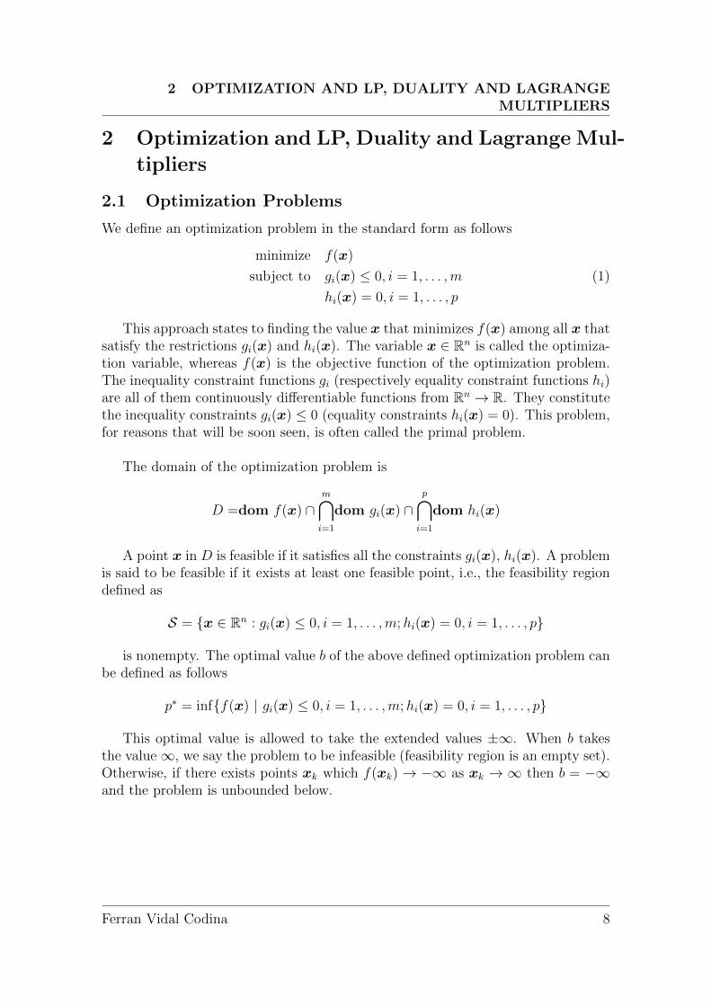
We define an optimization problem in the standard form as follows
minimize f(x)
subject to gi(x) ≤ 0, i = 1, . . . ,m (1)
hi(x) = 0, i = 1, . . . , p
This approach states to finding the value x that minimizes f(x) among all x thatsatisfy the restrictions gi(x) and hi(x). The variable x ∈ Rn is called the optimiza-tion variable, whereas f(x) is the objective function of the optimization problem.The inequality constraint functions gi (respectively equality constraint functions hi)are all of them continuously differentiable functions from Rn → R. They constitutethe inequality constraints gi(x) ≤ 0 (equality constraints hi(x) = 0). This problem,for reasons that will be soon seen, is often called the primal problem.
The domain of the optimization problem is
D =dom f(x) ∩m⋂i=1
dom gi(x) ∩p⋂
i=1
dom hi(x)
A point x in D is feasible if it satisfies all the constraints gi(x), hi(x). A problemis said to be feasible if it exists at least one feasible point, i.e., the feasibility regiondefined as
S = {x ∈ Rn : gi(x) ≤ 0, i = 1, . . . ,m;hi(x) = 0, i = 1, . . . , p}
is nonempty. The optimal value b of the above defined optimization problem canbe defined as follows
p∗ = inf{f(x) | gi(x) ≤ 0, i = 1, . . . ,m;hi(x) = 0, i = 1, . . . , p}
This optimal value is allowed to take the extended values ±∞. When b takesthe value∞, we say the problem to be infeasible (feasibility region is an empty set).Otherwise, if there exists points xk which f(xk) → −∞ as xk → ∞ then b = −∞and the problem is unbounded below.
Ferran Vidal Codina 8
2 OPTIMIZATION AND LP, DUALITY AND LAGRANGEMULTIPLIERS
2.2 Lagrange dual function and duality
2.2.1 Lagrangian
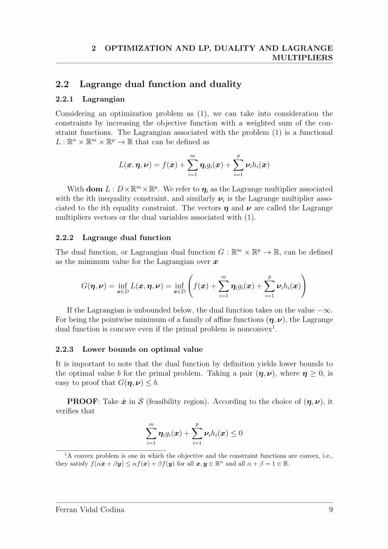
Considering an optimization problem as (1), we can take into consideration theconstraints by increasing the objective function with a weighted sum of the con-straint functions. The Lagrangian associated with the problem (1) is a functionalL : Rn × Rm × Rp → R that can be defined as
L(x,η,ν) = f(x) +m∑i=1
ηigi(x) +
p∑i=1
νihi(x)
With dom L : D×Rm×Rp. We refer to ηi as the Lagrange multiplier associatedwith the ith inequality constraint, and similarly νi is the Lagrange multiplier asso-ciated to the ith equality constraint. The vectors η and ν are called the Lagrangemultipliers vectors or the dual variables associated with (1).
2.2.2 Lagrange dual function
The dual function, or Lagrangian dual function G : Rm × Rp → R, can be definedas the minimum value for the Lagrangian over x
G(η,ν) = infx∈D
L(x,η,ν) = infx∈D
(f(x) +
m∑i=1
ηigi(x) +
p∑i=1
νihi(x)
)
If the Lagrangian is unbounded below, the dual function takes on the value −∞.For being the pointwise minimum of a family of affine functions (η,ν), the Lagrangedual function is concave even if the primal problem is nonconvex1.
2.2.3 Lower bounds on optimal value
It is important to note that the dual function by definition yields lower bounds tothe optimal value b for the primal problem. Taking a pair (η,ν), where η ≥ 0, iseasy to proof that G(η,ν) ≤ b.
PROOF: Take x in S (feasibility region). According to the choice of (η,ν), itverifies that
m∑i=1
ηigi(x) +
p∑i=1
νihi(x) ≤ 0
1A convex problem is one in which the objective and the constraint functions are convex, i.e.,they satisfy f(αx+ βy) ≤ αf(x) + βf(y) for all x,y ∈ Rn and all α+ β = 1 ∈ R.
Ferran Vidal Codina 9
2 OPTIMIZATION AND LP, DUALITY AND LAGRANGEMULTIPLIERS
as gi(x) ≤ 0 and hi(x) = 0, whereby every term of the first sum is nonpositiveand every term of the second is equal to zero.
Thus, evaluating the Lagrangian on x, we obtain L(x,η,ν) ≤ f(x). Automat-ically, we have G(η,ν) = inf L(x,η,ν) ≤ L(x,η,ν) ≤ f(x). Since this inequalityholds for any feasible point, the proof is complete.�
Hence, the following inequality verifies
G(η,ν) ≤ infg(x)≤0h(x)=0
f(x) (2)
Nevertheless, it should be taken into account that if G(η,ν) = −∞ the lowerbound is trivial. Hence, for a nontrivial lower bound for b need to be η ≥ 0. Ifthe pair (η,ν) attain to this condition, they belong to the dual feasibility region T ,which contains the pairs (η,ν) such that the dual function is not unbounded below.
2.2.4 The Lagrange dual problem
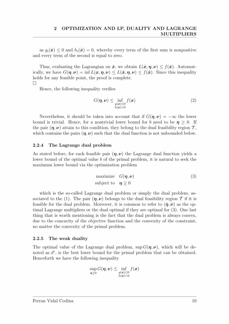
As stated before, for each feasible pair (η,ν) the Lagrange dual function yields alower bound of the optimal value b of the primal problem, it is natural to seek themaximum lower bound via the optimization problem
maximize G(η,ν) (3)
subject to η ≥ 0
which is the so-called Lagrange dual problem or simply the dual problem, as-sociated to the (1). The pair (η,ν) belongs to the dual feasibility region T if it isfeasible for the dual problem. Moreover, it is common to refer to (η, ν) as the op-timal Lagrange multipliers or the dual optimal if they are optimal for (3). One lastthing that is worth mentioning is the fact that the dual problem is always convex,due to the concavity of the objective function and the convexity of the constraint,no matter the convexity of the primal problem.
2.2.5 The weak duality
The optimal value of the Lagrange dual problem, supG(η,ν), which will be de-noted as d∗, is the best lower bound for the primal problem that can be obtained.Henceforth we have the following inequality
supη≥0
G(η,ν) ≤ infg(x)≤0h(x)=0
f(x)
Ferran Vidal Codina 10
2 OPTIMIZATION AND LP, DUALITY AND LAGRANGEMULTIPLIERS
which stands even if the problem is not convex. This property is known as theweak duality. The weak duality holds even in case one of the inequality members isinfinite. For example, if the dual problem is unbounded above (supG(η,ν) =∞),the primal problem is infeasible, i.e. p∗ =∞. Otherwise, if the primal is unboundedbelow (p∗ = −∞), the dual must be infeasible (supG(η,ν) = −∞).
We refer to the difference between both quantities, p∗− d∗, as the optimal dual-ity gap, which is the gap between the optimal value of the primal problem and thegreatest lower bound, and it is always nonnegative.
The weak duality can be used to find lower bounds of the primal problem, and itis useful in cases where the primal is difficult to solve, as the dual is always convex.
2.2.6 The strong duality
If the optimal duality gap is zero, the strong duality holds. If the primal problemis convex, then the strong duality usually (but not always) holds. A primal convexproblem is as follows
minimize f(x)
subject to gi(x) ≤ 0, i = 1, . . . ,m
Ax = b
Where f(x) and gi(x) are convex. Many results can be found about establishingconditions under which strong duality holds, but there will be no further discussedin this project.
2.3 Linear optimization problems
2.3.1 LP in standard form, its dual and extended dual theorem
When the objective and the constraint functions in our optimization problem arelinear2, the problem is called a Linear Program (LP). A standard LP problem canbe written as
minimize cTx
subject to Ax = b
x ≥ 0
with the only equalities as the component-wise nonnegativity constraints. Lin-ear programs are, of course, convex optimization problems. Since it is possible tomaximize an affine objective function cTx by minimizing −cTx (convex as well),
2A linear function is one that satisfies f(αx + βy) = αf(x) + βf(y) for all x,y ∈ Rn and allα, β ∈ R.
Ferran Vidal Codina 11
2 OPTIMIZATION AND LP, DUALITY AND LAGRANGEMULTIPLIERS
it is also referred as a LP a maximization problem with linear objective and con-straint functions. It should be noted that in this case the feasible set is a generalizedpolyhedron P , and the problem is to minimize the affine function cTx over P . Theproblem dual to this latter is
maximize uTb
subject to uTA ≤ cT
With this definitions it is immediate that
LEMMA 2.1 If Ax = b,uTA ≤ cT then
uTb = uTAx ≤ cTx
Finally is announced the dual theorem, first conjectured by J. von Neumann andproved afterwards by Gale, Kuhn and Tucker, of LP.
Theorem 2.1 (Extended dual theorem) For any dual pair of problems, pre-cisely one of the following occurs:
1. There exists x∗,u∗ with Ax∗ = b,x∗ ≥ 0 and u∗TA ≤ cT such that u∗T =cTx∗
2. Ax = b,x ≥ 0 has a solution, uTA ≤ cT has none and min cTx = −∞
3. Ax = b,x ≥ 0 has no solution, uTA ≤ cT has one and maxuTb =∞
4. Neither Ax = b,x ≥ 0 nor uTA ≤ cT have a solution
COROLLARY 2.1 If Ax = b,x ≥ 0 has a solution and cTx is bounded below(or alternatively if uTA ≤ cT has a solution and uTb is bounded above) then thereexists optimal solutions x∗,u∗ to both problems above.
2.3.2 LP in general form, lagrangian and duality
A general linear program can be expressed as
minimize cTx
subject to Dx ≤ e (4)
Ax = b
And the variables x, c ∈ Rn, e ∈ Rm,b ∈ Rp,D ∈ Rm×n and A ∈ Rp×n. TheLagrangian L : Rn × Rm × Rp → R associated to (4) can be defined as
L(x,η,ν) = cTx+ηT (Dx−e)+νT (Ax−b) = −eTη−bTν+xT (DTη+ATν+c)
Ferran Vidal Codina 12
3 EVOLUTION IN LIMIT ANALYSIS TECHNIQUES
so the dual function is
G(η,ν) = infxL(x,η,ν) = −eTη − bTν + inf
x(xT (DTη + ATν + c))
The infimum of a linear function is −∞, except in the case where is identicallyzero, so the dual function can be expressed as
G(η,ν) =
{−eTη − bTν if DTη + ATν + c = 0−∞ otherwise
The dual variable η is dual feasible if η ≥ 0 and DTη+ ATν + c = 0, hence thelower bound property (2) holds, and the lower bound to the optimal value happens tobe −eTη−bTν (4). The Lagrange dual problem defined by (3) can be reformulatedby including the dual feasibility conditions as explicit constraints
maximize − eTη − bTν
subject to DTη + ATν + c = 0 (5)
η ≥ 0
The problem that will be dealt throughout this project responds to problems (4)and (5). Nevertheless, many different forms of LP problems can be used dependingon the LP solver chosen (linsolve, SDPT3, CVX,. . . ) and the very nature of theproblem itself. Further information about LP problems approaches can be found in[1].
3 Evolution in limit analysis techniques
Limit analysis has been an increasingly and widely used tool for structure design-ing and soil mechanics analysis since its initial developments in the 19th century.The problem aimed to be solved by means of limit analysis consists of finding theminimum multiple of the load distribution in a solid subject that drives to the com-plete collapse of the body, assuming a plastic behavior of the subject, i.e. elasticrange is left. In this project it will be discussed the limit analysis applied to findingconditions of failure of statically loaded 3D and 2D-structures of ductile materi-als, particularly steel, and the process of loading will be proportional. Continuousbeams and frames of steel can carry loads considerably greater than the ones whichcause to reach the elastic limit of the material. In general, when loading increasesplastic yield is attained in some elements of the structure, which implies the par-tial loss of its bearing capacities. If the process of loading does not cease it mayincur the physical failure of the structure, when the load has reached a certain valuecalled collapse load. Above this factor, small loading increases may result in muchlarger permanent deformations than the ones experienced before. The so-called plas-tic methods attempt to estimate the collapse load factor, and hence provide both a
Ferran Vidal Codina 13
3 EVOLUTION IN LIMIT ANALYSIS TECHNIQUES
knowledge of its bearing capacity and a better use of materials in the design process.
Plastic analysis is based on the idealization of the stress-strain surface as elastic-perfectly-plastic. The relation between the bending moment and the curvature ateach member of the structure is the starting point for the limit analysis. The basichypothesis is that if the bending moment of an initially unstressed and unstrainedelement under pure bending approaches a value noted by Mp, which depends on thenature and characteristics of the material, the curvature of the element increasesindefinitely. This value is commonly referred to as the plastic moment of the mem-ber. The formation of a plastic hinge is closely related to the attainment of theplastic moment in some sections. The concept of plastic hinge, which is key in limitanalysis, was first proposed according to Maier-Leibnitz [2] by G.V.Kazinczy in theHungarian journal Betonszemble in 1914. Theoretically, if the plastic moment isreached in a section of a member it would lead to infinite curvature, hence this sec-tion would be able to change the slope angle in infinitesimal distances. Hence themembers would behave as if they were attached to a hinge which transmits only aconstant moment equal to ±Mp.
Progresses in the development of efficient plastic methods for limit analysis cal-culation were made by Greenberg and Prager [3], and the most relevant ones thatshould be pointed out are the static and kinematic theorem. Let Pc be the actualcollapse load of a given frame, accepting that all the loads can be combined withcertain ratios so that can be expressed as a single quantity. Admit Plb as a load atwhich it is possible to find a feasible system of bending moments satisfying equi-librium equations and plastic moment is not reached at any section. Under thesecircumstances, Greenberg and Prager showed that Plb ≤ Pc.
This kinematic method is based on the combination of elementary mechanismsand the virtual work principle. The plastic collapse loads correspond to several fail-ure mechanisms, and are found by equating the internal work at the plastic hingeswith the external work performed by the loads during the virtual displacement.Rotations and deflections must thereby be computed. One of the hypotheses as-sumed is that the frame remains rigid between the supports and the hinges, thusplastic rotation only occurs at plastic hinges. Combining mechanisms various col-lapse loads can be found, and the kinematic theorem states that the minimum loadfactor is an upper bound of the real collapse load. Its immediate consequence isthat Pc ≤ Pub, where Pub is the minimum load found combining mechanisms. Thismethod constitutes a useful tool for having an reference value of the load necessaryfor a structure to lose its stability and collapse, but it always yields to unsafe values.Thus, considering both principles the following inequality can be obtained
Plb ≤ Pc ≤ Pub
Which expresses that there one and only one collapse load: there exists a uniqueload value such tat, with all bending moments satisfying statical equilibrium and
Ferran Vidal Codina 14
3 EVOLUTION IN LIMIT ANALYSIS TECHNIQUES
nowhere exceeding a plastic moment magnitude, plastic hinges exist at sufficientsections to convert the frame into a kinematic mechanism. This load can only befound explicitly if the results of both static and kinematic principles coincide. Themethodology of collapse load calculation based on these theorems was developedand widespread by Symonds and Neal [4, 5].
Symonds and Neal [6] were also relevant for their studies about computationof plastic moments of various cross sections and techniques for its computation ingeneral cases. Moreover, observations were made regarding the influence of shearstress and axial forces on the variation of the plastic moment, and together withChwalla [7], Baker, Horne and Roderick [8] further investigations were carried outconcerning conditions under which these forces should be taken into account.
Paralelly to the demonstration of these two theorems in 1951, which revealed tobe crucial in the development and study of limit analysis, it gained relevance theapproach to the problem of finding the exact collapse load as a linear programmingproblem. It had been studied previously, but it always appeared the obstacle of aphysical interpretation of the variables intervening in the dual problem. Charnes andGreenberg [9] established the equivalence, for trussed structures, of dual program-ming problems and the static and kinematic theorems. This equivalence regardedthe stress in a bar as a primal variable and the displacement of a joint as a dualvariable. Henceforth, these identification allowed the study of trussed structuresusing the theory and the computational advantages of linear programming.
The conjectured equivalence for frames, the most important structural applica-tion, was not proved until 1959 by Charnes, Lemke and Zienkiewicz [10] using virtualwork and geometric compatibility. In this article the authors developed a parametricform for the static equations of equilibrium combined with the compatibility condi-tions, as well as giving a physical interpretation of the dual variables. Using theseresults, the LP problem was first formulated, being the primal the maximization ofthe load factor subject to the statical equilibrium equations (static theorem), andits dual the minimization of the load factor subject to the conditions of constitutinga kinematic mechanism attaining the plastic moment at the critical sections. It fol-lows by the application of the extended dual theorem (2.1) that it there is a finiteoptimum for either the primal or the dual, then there must be one for the other.As a consequence of this duality and the application of the extended dual theoremconditions for the existence of a collapse mechanism were stablished.
Once the LP problem was formulated, further progresses were made in this field,aiming to improve the approach to the actual problem and the solving techniques.There should be cited Heyman [11], Horne [12], Baker and Heyman [13] and Wat-wood [14]. In 1972, Anderheggen and Knopfel [15] first introduced in the problemof finding the collapse load factor the necessity of a combined yield condition. Be-forehand it was only taken into account the influence of the bending moment as a
Ferran Vidal Codina 15
3 EVOLUTION IN LIMIT ANALYSIS TECHNIQUES
condition for attaining plastic flow with the aforementioned plastic hinges. It hadbeen noted the negative influence of axial and shear forces on the fully plastic mo-ment, but no mathematical approach had been made. Anderheggen and Knopfelintroduced the yield condition as a feasible stress domain in the bending moment -axial force plane (in two dimensions) that should not be violated at any point. As itwill be seen throughout this project, yield surfaces are in general nonlinear convexsets, therefore a process of linearization of the yield conditions was proposed. Bymeans of this process the restriction of not exceeding the (reduced) plastic momentcould be placed as a constraint in the LP primal problem. Furthermore, the finiteelement method was used as a mathematical tool for modeling the problem andformulating it as an LP, by assuming stress and displacement fields and then usingthe virtual work principle to find the coefficients corresponding to linear equilibriumand kinematic compatibility.
This latter article set the basis of finding the collapse load factor as it is statednowadays. Other referent authors which contributed to the development of solvingthe LP problem were Munro [16], Livesley [17] and Maier, Giacomini and Pater-lini [18]. The results achieved by the last quoted authors involve formulating theproblem as a restricted basis linear program (RBLP), which implicates that in thebasic LP problem there is an extra complementarity nonlinear condition, able to besolved by the standard simplex method with a similar computational cost, althoughit provided the deformation history of the structure.
Jennings and Tam [19] proposed in their paper a modified simplex techniquebased on a minimum weight criteria for the selection of relative member sizes, forstructures with only flexural actions and concentrated loads, minimizing an objec-tive function which regards the possible positions of the plastic hinges and checksequilibrium via the static theorem. Further innovations in methods of solving theproblem can be attributed to Thierauf [20], who presented an iterative method forsolving the limit analysis problem with alternative loads with a linear objectivefunction and quadratic yield conditions.
Damkilde and Hoyer [21] proposed a new approach to the standard LP problembased on the reduction of degrees of freedom a priori so as to deal with a reducedproblem with less equations and also the LP problem without the restriction of non-negative variables (which is actually more accurate) using slack variables. Damkildeused the linearization of the yield surface as well, thus checking yield conditionsare not violated at any point. Another interesting idea stated in this paper wasthe possibility of the inclusion of the material optimization, so a double load andmaterial optimization can be carried out.
From the early 90s until nowadays great progresses have been made in solv-ing the collapse load factor problem using different computer approaches. For in-stance, Tin-Loi [22] used the mathematical programming language GAMS for pla-
Ferran Vidal Codina 16
4 LIMIT STATE ANALYSIS AS A LP PROBLEM
nar frames; Kaveh and Jahanshahi [23] applicated heuristic algorithms such as AntColony System; Corradi, Luzzi and Vena [24] developed the limit analysis problemfor anisotropic structures; Tjhin and Kuchma [25] used the strut-and-tie method asan equilibrium method for the limit analysis; Van Long and Dan Hung [26] com-bined direct LP methods with step-by-step methods for the analysis of 3D frames;Peraire, Bonet and Ciria [27] designed a program with an adaptive mesh system forthe computation of both lower and upper bounds, solving in this case second-ordercone programs.
Furthermore, if the focus is on the evolution of the LP solving techniques, authorssuch as Borges et al.[28], Lyamin [29], and Krabbenhoft and Damkilde [30] madedecisive apportations with much more efficient methods than the simplex methods,which are capable of solving both linear and nonlinear programs. In addition tothat, in these methods the number of iterations is largely independent of the prob-lem size, meaning that problems with thousands of variables can be solved withinminutes.
As stated before, this project will focus on the development of limit analysis ofboth trussed and framed 3D and 2D structures writing it as a LP problem. Firstlyglobal equilibrium equations will be introduced in matrix notation, bearing in mindgeometric restrictions and kinematic constraints. One of the new approaches to theproblem is the yield condition linearization. Yield surface of standard beam cross-sections is explicitly written, and it is adaptively approximated in a manner thatevery element of the structure can have its yield surface differently approximatedif desired. Besides that, this approximation yields to lower and upper bounds ofthe exact collapse load whether the yield surface (always convex) is approximatedinwards or outwards. The second major innovation is the possibility of consideringuniform distributed loads, and an adaptive procedure is sought as well. Combiningboth the yield conditions, UDL and adaptivity the bound gap can be arbitrarilyreduced, and therefore a more precise collapse load factor can be found.
4 Limit state analysis as a LP problem
Following some of the aforementioned developments and work in limit analysis, ageneral and complete approach to the problem of finding the exact load factor thatscales the external loadings in order to induce collapse to the structure is explicitlyproposed here. This load factor, which will be referenced from now on using thenotation λ, is forced to be nonnegative, thus the direction of the loads is decisive.This procedure is based on the static theorem, which states that a given staticallyadmissible stress distribution which doesn’t violate yield criteria anywhere inducesa lower-bound of the actual collapse load. This condition will therefore be expressedas a LP problem. Its dual problem, which happens to be the kinematic theorem,will not be sought in this project, nevertheless it would lead to the same exact result
Ferran Vidal Codina 17
4 LIMIT STATE ANALYSIS AS A LP PROBLEM
(with a sensible stress and displacement fields and accounting the fact that the dualof the dual is again the primal problem). However, for a computer-based approachit is simpler to consider the static theorem. In this section the equilibrium equationsand yield criteria will be presented, as well as its writing as linear conditions for itsfurther use in the LP problem.
1
2y
x
z
N
M1y
M1z
Mx
Mx
M2y
M2z
N
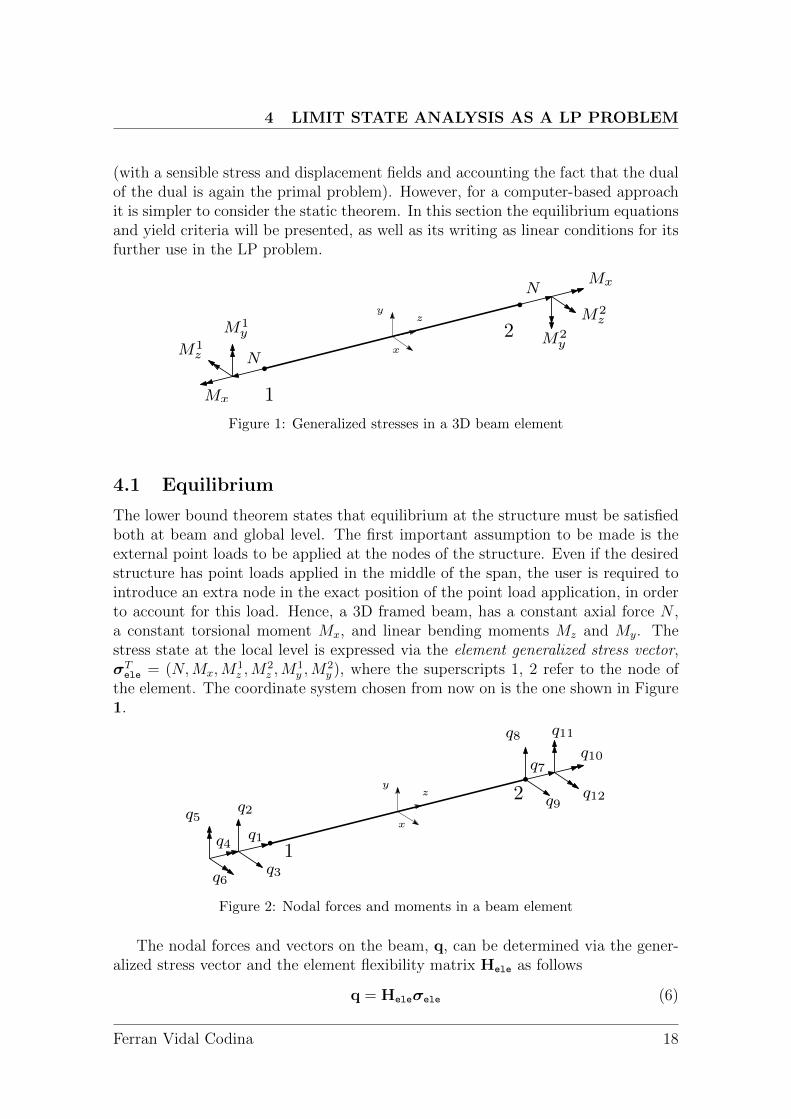
Figure 1: Generalized stresses in a 3D beam element
4.1 Equilibrium
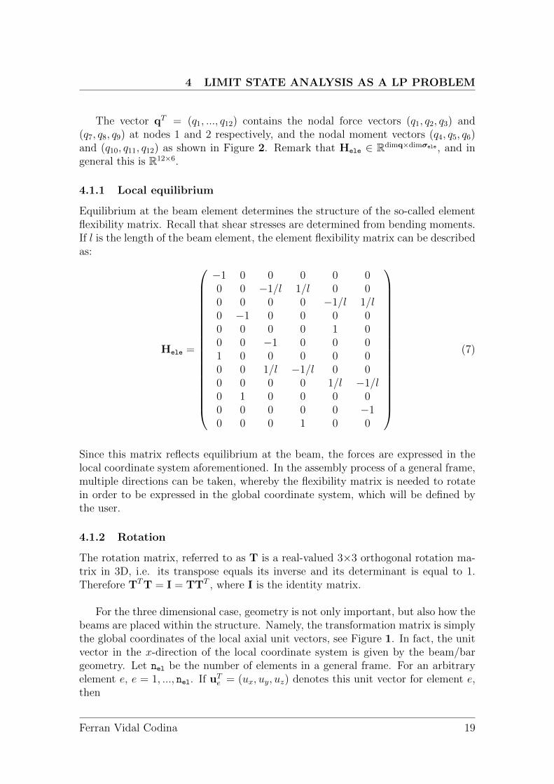
The lower bound theorem states that equilibrium at the structure must be satisfiedboth at beam and global level. The first important assumption to be made is theexternal point loads to be applied at the nodes of the structure. Even if the desiredstructure has point loads applied in the middle of the span, the user is required tointroduce an extra node in the exact position of the point load application, in orderto account for this load. Hence, a 3D framed beam, has a constant axial force N ,a constant torsional moment Mx, and linear bending moments Mz and My. Thestress state at the local level is expressed via the element generalized stress vector,σTele = (N,Mx,M
1z ,M
2z ,M
1y ,M
2y ), where the superscripts 1, 2 refer to the node of
the element. The coordinate system chosen from now on is the one shown in Figure1.
1
2y
x
z
q1
q2
q3
q4
q5
q6
q7
q8
q9
q10
q11
q12
Figure 2: Nodal forces and moments in a beam element
The nodal forces and vectors on the beam, q, can be determined via the gener-alized stress vector and the element flexibility matrix Hele as follows
q = Heleσele (6)
Ferran Vidal Codina 18
4 LIMIT STATE ANALYSIS AS A LP PROBLEM
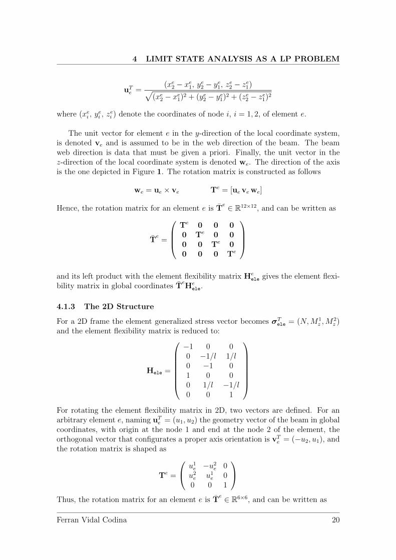
The vector qT = (q1, ..., q12) contains the nodal force vectors (q1, q2, q3) and(q7, q8, q9) at nodes 1 and 2 respectively, and the nodal moment vectors (q4, q5, q6)and (q10, q11, q12) as shown in Figure 2. Remark that Hele ∈ Rdimq×dimσele , and ingeneral this is R12×6.
4.1.1 Local equilibrium
Equilibrium at the beam element determines the structure of the so-called elementflexibility matrix. Recall that shear stresses are determined from bending moments.If l is the length of the beam element, the element flexibility matrix can be describedas:
Hele =
−1 0 0 0 0 00 0 −1/l 1/l 0 00 0 0 0 −1/l 1/l0 −1 0 0 0 00 0 0 0 1 00 0 −1 0 0 01 0 0 0 0 00 0 1/l −1/l 0 00 0 0 0 1/l −1/l0 1 0 0 0 00 0 0 0 0 −10 0 0 1 0 0
(7)
Since this matrix reflects equilibrium at the beam, the forces are expressed in thelocal coordinate system aforementioned. In the assembly process of a general frame,multiple directions can be taken, whereby the flexibility matrix is needed to rotatein order to be expressed in the global coordinate system, which will be defined bythe user.
4.1.2 Rotation
The rotation matrix, referred to as T is a real-valued 3×3 orthogonal rotation ma-trix in 3D, i.e. its transpose equals its inverse and its determinant is equal to 1.Therefore TTT = I = TTT , where I is the identity matrix.
For the three dimensional case, geometry is not only important, but also how thebeams are placed within the structure. Namely, the transformation matrix is simplythe global coordinates of the local axial unit vectors, see Figure 1. In fact, the unitvector in the x-direction of the local coordinate system is given by the beam/bargeometry. Let nel be the number of elements in a general frame. For an arbitraryelement e, e = 1, ..., nel. If uT
e = (ux, uy, uz) denotes this unit vector for element e,then
Ferran Vidal Codina 19
4 LIMIT STATE ANALYSIS AS A LP PROBLEM
uTe =
(xe2 − xe1, ye2 − ye1, ze2 − ze1)√(xe2 − xe1)2 + (ye2 − ye1)2 + (ze2 − ze1)2
where (xei , yei , z
ei ) denote the coordinates of node i, i = 1, 2, of element e.
The unit vector for element e in the y-direction of the local coordinate system,is denoted ve and is assumed to be in the web direction of the beam. The beamweb direction is data that must be given a priori. Finally, the unit vector in thez-direction of the local coordinate system is denoted we. The direction of the axisis the one depicted in Figure 1. The rotation matrix is constructed as follows
we = ue × ve Te = [ue ve we]
Hence, the rotation matrix for an element e is Te ∈ R12×12, and can be written as
Te
=
Te 0 0 00 Te 0 00 0 Te 00 0 0 Te
and its left product with the element flexibility matrix He
ele gives the element flexi-bility matrix in global coordinates T
eHe
ele.
4.1.3 The 2D Structure
For a 2D frame the element generalized stress vector becomes σTele = (N,M1
z ,M2z )
and the element flexibility matrix is reduced to:
Hele =
−1 0 00 −1/l 1/l0 −1 01 0 00 1/l −1/l0 0 1
For rotating the element flexibility matrix in 2D, two vectors are defined. For anarbitrary element e, naming uT
e = (u1, u2) the geometry vector of the beam in globalcoordinates, with origin at the node 1 and end at the node 2 of the element, theorthogonal vector that configurates a proper axis orientation is vT
e = (−u2, u1), andthe rotation matrix is shaped as
Te =
u1e −u2e 0u2e u1e 00 0 1
Thus, the rotation matrix for an element e is T
e ∈ R6×6, and can be written as
Ferran Vidal Codina 20
4 LIMIT STATE ANALYSIS AS A LP PROBLEM
Te
=
(Te 00 Te
)and the element flexibility matrix in global coordinates is defined by left multi-
plying with this latter matrix.
4.1.4 Equilibrium for trusses
It was regarded important to remark the simple case where the structure has hingesat every node. The elements only carry axial loads, therefore σele = N ∈ R and theelement flexibility matrix is HT
ele = (−1, 0, 1, 0) in 2D and HTele = (−1, 0, 0, 1, 0, 0)
in 3D.
4.1.5 Global equilibrium
Once local equilibrium is clarified, the next step is equilibrium for the whole struc-ture. Nodal equilibrium for the global frame is determined after summation of theelement contributions at the nodes, the so-called p vectors in (6), and the externalloads. The several element flexibility matrices defined in (7) must be assembled inthe global flexibility matrix H, and accounting the external loads and the reactionforces due to kinematic constraints, global equilibrium can be expressed as follows
Hσ = Gr + λf (8)
where f is the vector containing all the external nodal forces3, λ is the plasticload multiplier (the aim of the problem), r is the vector containing the reactionsdue to the boundary conditions and kinematic constraints and G is a matrix thatrelates each reaction force to the corresponding geometric restriction (embedded,simply supported,...). σ is the global generalized stress vector, which contains allthe element stress vector assembled, therefore
σ = (σ1ele
T, ...,σnel
eleT )
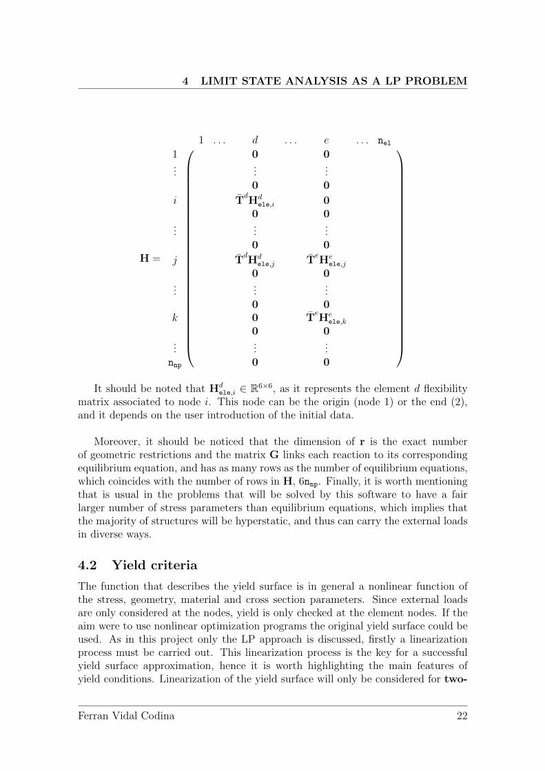
This vector belongs to R6nel but need not to have this exact dimension sincestatic constraints such as internal hinges can be present in the structure, and thestress parameters can be known a priori and the dimension of σ must be reducedaccordingly. The number of columns of H is equal to the dimension of σ; thus ingeneral is six times the number of elements, 6nel. The number of rows correspondsto nodal equilibrium for each degree of freedom. In general it is six times the numberof nodal points, 6nnp. The structure of the global flexibility matrix can be written,where rows represent nodes and columns represent elements, as follows
3UDL inclusion will be later discussed.
Ferran Vidal Codina 21
4 LIMIT STATE ANALYSIS AS A LP PROBLEM
H =
1 . . . d . . . e . . . nel1 0 0...
......
0 0
i TdHd
ele,i 00 0
......
...0 0
j TdHd
ele,j TeHe
ele,j
0 0...
......
0 0k 0 T
eHe
ele,k
0 0...
......
nnp 0 0
It should be noted that Hd
ele,i ∈ R6×6, as it represents the element d flexibilitymatrix associated to node i. This node can be the origin (node 1) or the end (2),and it depends on the user introduction of the initial data.
Moreover, it should be noticed that the dimension of r is the exact numberof geometric restrictions and the matrix G links each reaction to its correspondingequilibrium equation, and has as many rows as the number of equilibrium equations,which coincides with the number of rows in H, 6nnp. Finally, it is worth mentioningthat is usual in the problems that will be solved by this software to have a fairlarger number of stress parameters than equilibrium equations, which implies thatthe majority of structures will be hyperstatic, and thus can carry the external loadsin diverse ways.
4.2 Yield criteria
The function that describes the yield surface is in general a nonlinear function ofthe stress, geometry, material and cross section parameters. Since external loadsare only considered at the nodes, yield is only checked at the element nodes. If theaim were to use nonlinear optimization programs the original yield surface could beused. As in this project only the LP approach is discussed, firstly a linearizationprocess must be carried out. This linearization process is the key for a successfulyield surface approximation, hence it is worth highlighting the main features ofyield conditions. Linearization of the yield surface will only be considered for two-
Ferran Vidal Codina 22

4 LIMIT STATE ANALYSIS AS A LP PROBLEM
dimensional frames, since the 3D case is still being implemented. Thus, form nowon yield criteria will be referred as yield curve rather than yield curve.
4.2.1 Class type
According to its behavior facing normal stress, the cross section of a beam elementin a structure can be classified as follows
1. Plastic
2. Compact
3. Semi-compact
4. Slender
This classification provides an average idea of how much local instability (dent)which arise during the process of loading can be capable of limiting both the strengthof the cross section (moment that can be reached without collapsing) and its rota-tion capability (curvature that can be adopted without collapsing).
Depending on the sensitivity of a cross section to bear with local instabilitiesfour types or section classes can be defined:
� Class 1 (plastic) sections are capable of not only reaching its fully plasticmoment without arising instability problems, but also have enough rotationcapacity to form a plastic hinge, and allow the perfect plasticity behaviordemanded for a global plastic analysis.
� Class 2 (compact) sections are capable of reaching its fully plastic momentwithout arising instability problems, although don’t have enough rotation ca-pacity to form a plastic hinge for a global plastic analysis. As a consequenceof this latter fact, in isostatical structures the same global exploitation of thematerial as if it were a plastic section is permitted. However, material ex-ploitation in hyperstatical structures is strictly lower than the one that can beattained using plastic sections.
� Class 3 (semi-compact) sections present local dent problems before attain-ing the fully plastic moment and once surpassed the elastic moment. Thesection resistant moment will be considered equal to the elastic moment.
� Class 4 (slender) sections are incapable of even developing its elastic capacityin the most compressed metallic fiber, due to instabilities at the compressedsheets.
Ferran Vidal Codina 23

4 LIMIT STATE ANALYSIS AS A LP PROBLEM
The assignation of a class to a determined cross section involves a number ofparameters such as the material’s elastic limit, the geometry of the section, theslenderness of its fully or partially compressed panels and the loads at which thesection is undergone. Actually, the section type will be known a priori by usingthe various steel cross section catalogues available4, and as the functioning of thesoftware is shown this matter will be deepened.
4.2.2 Yield function definition
As stated before, plastic analysis only makes sense if considering cross sections withC1 or C2 collapse state, since these are the ones that attain plastic flow. Further-more, geometry of the cross section has revealed as a decisive factor in the nonlin-ear yield curve, thus it is crucial to analitically know its description of the mostcommonly used cross sections. This project will focus on the doubly symmetricI/H-shaped cross sections, basically the IPE and HEB series, due to its vast presencein steel structures and widespread use. Rectangular cross sections should also bementioned, but will be no further discussed as a rectangular solid steel section isseldom found. Nowadays only doubly symmetric I/H-shaped cross sections can befound on the Cross Section Library of the Structural Collapse Simulator, nonethe-less there are currently being implemented non-symmetric cross sections such as T, Uor L shape, as its yield function is found and the linearization procedure is developed.
b
z
y
hw h
tw
Figure 3: I/H-shaped symmetric cross section
Finding the yield curve definition in an axial force-bending moment cartesianplane consists of finding the relationship between N and M when the section under-goes combined bending and axial load, by forcing equilibrium in the zero strainaxis (ZSA). In a doubly symmetric I/H-shaped cross section, the axial tension(NT ) and compression (NC) forces that plastify the cross section with no bend-ing are NT = −NC = Np = (twhw + b(h − hw))σp where σp, the yield stress,is assumed to coincide in tension and compression due to symmetries. The plas-tic bending moment that induces a plastic hinge to form under pure bending is
4The Structural Collapse Simulator is based on the ArcelorMittal catalogues.
Ferran Vidal Codina 24
4 LIMIT STATE ANALYSIS AS A LP PROBLEM
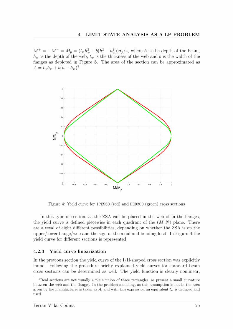
M+ = −M− = Mp = (twh2w + b(h2 − h2w))σp/4, where h is the depth of the beam,
hw is the depth of the web, tw is the thickness of the web and b is the width of theflanges as depicted in Figure 3. The area of the section can be approximated asA = twhw + b(h− hw)5.
−1 −0.8 −0.6 −0.4 −0.2 0 0.2 0.4 0.6 0.8 1−1
−0.8
−0.6
−0.4
−0.2
0
0.2
0.4
0.6
0.8
1
N/N
p
M/Mp
Figure 4: Yield curve for IPE550 (red) and HEB300 (green) cross sections
In this type of section, as the ZSA can be placed in the web of in the flanges,the yield curve is defined piecewise in each quadrant of the (M,N) plane. Thereare a total of eight different possibilities, depending on whether the ZSA is on theupper/lower flange/web and the sign of the axial and bending load. In Figure 4 theyield curve for different sections is represented.
4.2.3 Yield curve linearization
In the previous section the yield curve of the I/H-shaped cross section was explicitlyfound. Following the procedure briefly explained yield curves for standard beamcross sections can be determined as well. The yield function is clearly nonlinear,
5Real sections are not usually a plain union of three rectangles, as present a small curvaturebetween the web and the flanges. In the problem modeling, as this assumption is made, the areagiven by the manufacturer is taken as A, and with this expression an equivalent tw is deduced andused.
Ferran Vidal Codina 25
4 LIMIT STATE ANALYSIS AS A LP PROBLEM
although is interesting to notice from the yield curve depiction and from the generaltheory that every curve defines a convex set6 of feasible loads in the (M,N) plane.
For comodity it is advisable to work on a normalized plane, i.e. the
(M
Mp
,N
Np
)plane.
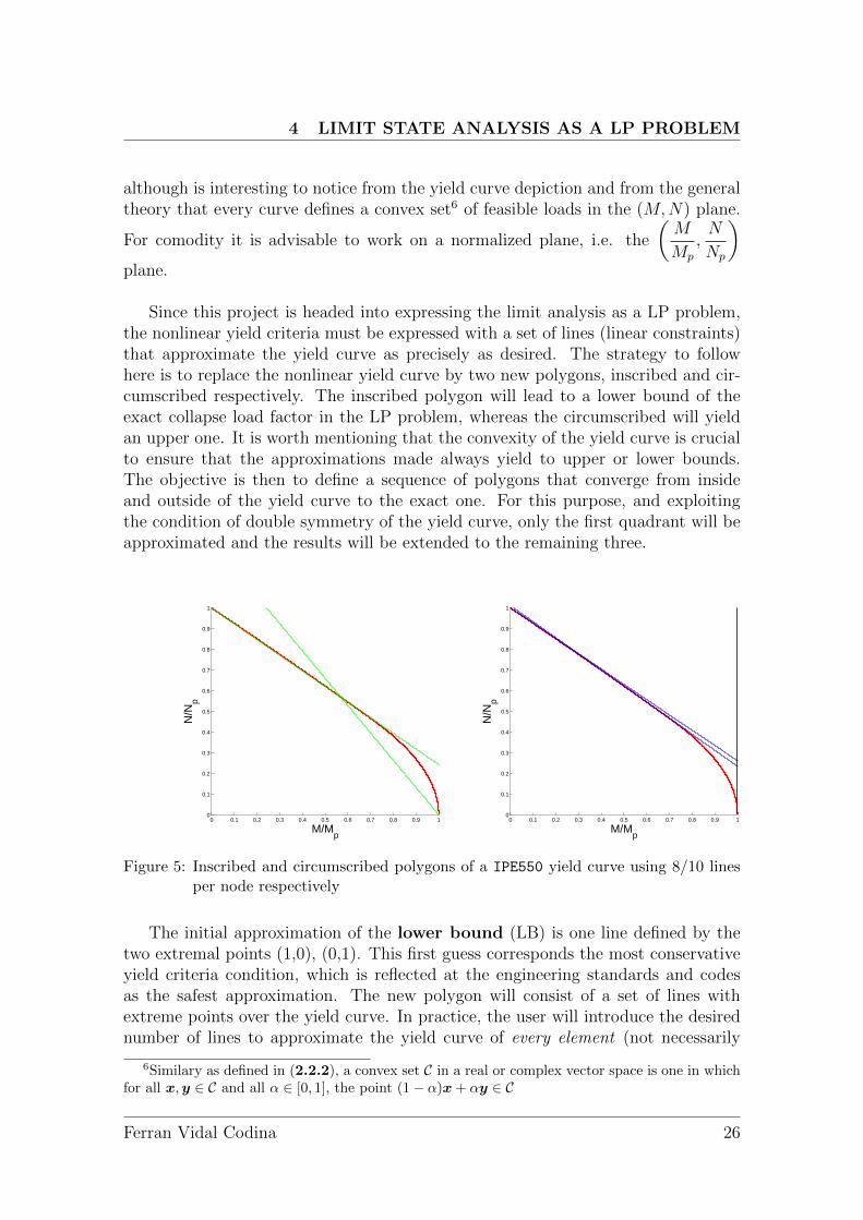
Since this project is headed into expressing the limit analysis as a LP problem,the nonlinear yield criteria must be expressed with a set of lines (linear constraints)that approximate the yield curve as precisely as desired. The strategy to followhere is to replace the nonlinear yield curve by two new polygons, inscribed and cir-cumscribed respectively. The inscribed polygon will lead to a lower bound of theexact collapse load factor in the LP problem, whereas the circumscribed will yieldan upper one. It is worth mentioning that the convexity of the yield curve is crucialto ensure that the approximations made always yield to upper or lower bounds.The objective is then to define a sequence of polygons that converge from insideand outside of the yield curve to the exact one. For this purpose, and exploitingthe condition of double symmetry of the yield curve, only the first quadrant will beapproximated and the results will be extended to the remaining three.
0 0.1 0.2 0.3 0.4 0.5 0.6 0.7 0.8 0.9 10
0.1
0.2
0.3
0.4
0.5
0.6
0.7
0.8
0.9
1
N/N
p
M/Mp
0 0.1 0.2 0.3 0.4 0.5 0.6 0.7 0.8 0.9 10
0.1
0.2
0.3
0.4
0.5
0.6
0.7
0.8
0.9
1
N/N
p
M/Mp
Figure 5: Inscribed and circumscribed polygons of a IPE550 yield curve using 8/10 linesper node respectively
The initial approximation of the lower bound (LB) is one line defined by thetwo extremal points (1,0), (0,1). This first guess corresponds the most conservativeyield criteria condition, which is reflected at the engineering standards and codesas the safest approximation. The new polygon will consist of a set of lines withextreme points over the yield curve. In practice, the user will introduce the desirednumber of lines to approximate the yield curve of every element (not necessarily
6Similary as defined in (2.2.2), a convex set C in a real or complex vector space is one in whichfor all x,y ∈ C and all α ∈ [0, 1], the point (1− α)x+ αy ∈ C
Ferran Vidal Codina 26
4 LIMIT STATE ANALYSIS AS A LP PROBLEM
the same lines for every element), with the only restriction to be a multiple of 4.The software will divide the first quadrant into sections with a beam of lines, andthe intersection between each one of these and the yield curve will determine pointsover the yield curve. Since the yield curve is the one previously defined, it canbe written as a compact function in the bending moment-axial force plane. As aconsequence, the procedure of finding the points is as simple as a Newton-Raphson1D technique to seek the abscissa where the difference between the yield curve andeach line vanishes. Due to symmetries a collection of points over the yield curve isavailable, whereby is trivial to define a set of lines that link two consecutive points,forming an inscribed polygon. Every point in and on the polygon is feasible becauseit is either in or on the yield curve. It is obvious that this latter fact leads to thecomputation of a lower bound of the exact collapse load.
The upper bound (UB) is computed similarly. However, in this case no Newton-Raphson is needed, as the strategy is to employ the collection of points found inthe lower bound approximation and define tangent lines to the yield curve at everypoint. It is worth noticing that in this procedure a notable step is found: the sin-
gularities at the points (0,1), (0,-1) of the
(M
Mp
,N
Np
)plane. The impossibility of
defining a tangent line at these points is solved by defining a right and left tangentline using the lateral derivatives of the yield function at a neighborhood of thesesingular points. Thereby a discrepancy arises when comparing to the lower boundapproximation; in the LB case n points define n lines, whereas in the UB case npoints define n + 2 points. However, this disagreement is properly treated in thesoftware. The points on the polygon are only feasible if they are on the yield curve,and obviously this approximation leads to unsafe load multipliers as the polygonis circumscribed in the actual yield curve. Nevertheless, this upper bound givesdecisive information on ”how good” the lower bound previously found is, i.e. theprecision of the first computation, which is certainly a matter of importance if astudy of convergence by creating a sequence of polygons is carried out.
In both cases the restrictions are linear, one restriction per edge of the polygon.Finally, this procedure expresses the linear restrictions in an adequate form for itsinclusion in the linear approximation of the yield criteria in the LP problem. Figure5 shows both the lower and upper approximation (first quadrant) of a IPE550 crosssection.
4.2.4 Yield criteria as a LP problem
The original nonlinear criteria would lead to a nonlinear optimization problem
f(N,Mx,Miz,M
iy) ≤ g(m1, . . . ,mk) i = 1, 2 (9)
Ferran Vidal Codina 27
4 LIMIT STATE ANALYSIS AS A LP PROBLEM
Mz
My
N
NC
NT
M+z
M−z
M+y
M−y
NT
M−M+
NC
N
M
Figure 6: Simplest linearization for a general yield surface
where m1, . . . ,mk are the material parameters that characterize the beam prop-erties and the material, which can of course be different for every element. Toperform the computation as a LP problem this criteria is linearized following theprocedure described in the previous section. The case treated in this project is onlyconcerned in finding the factor that maximizes the external load so as to inducecollapse in the structure. Therefore only the left-hand side of (9) must be linearizedand optimized. If the aim were to optimize the material resources for a given load,the inverse process should be carried out. For each element, the condition of notexceeding yield curve can be expressed as
Fi
NM i
z
M iy
≤ gi for i = 1, 2
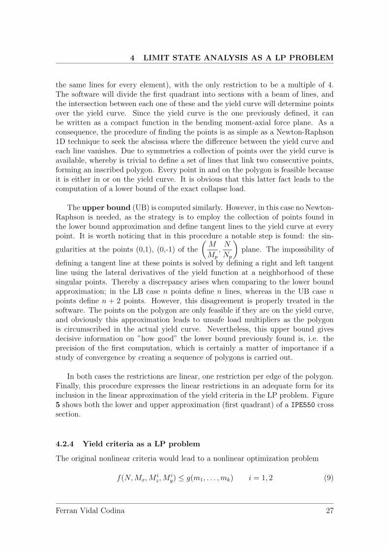
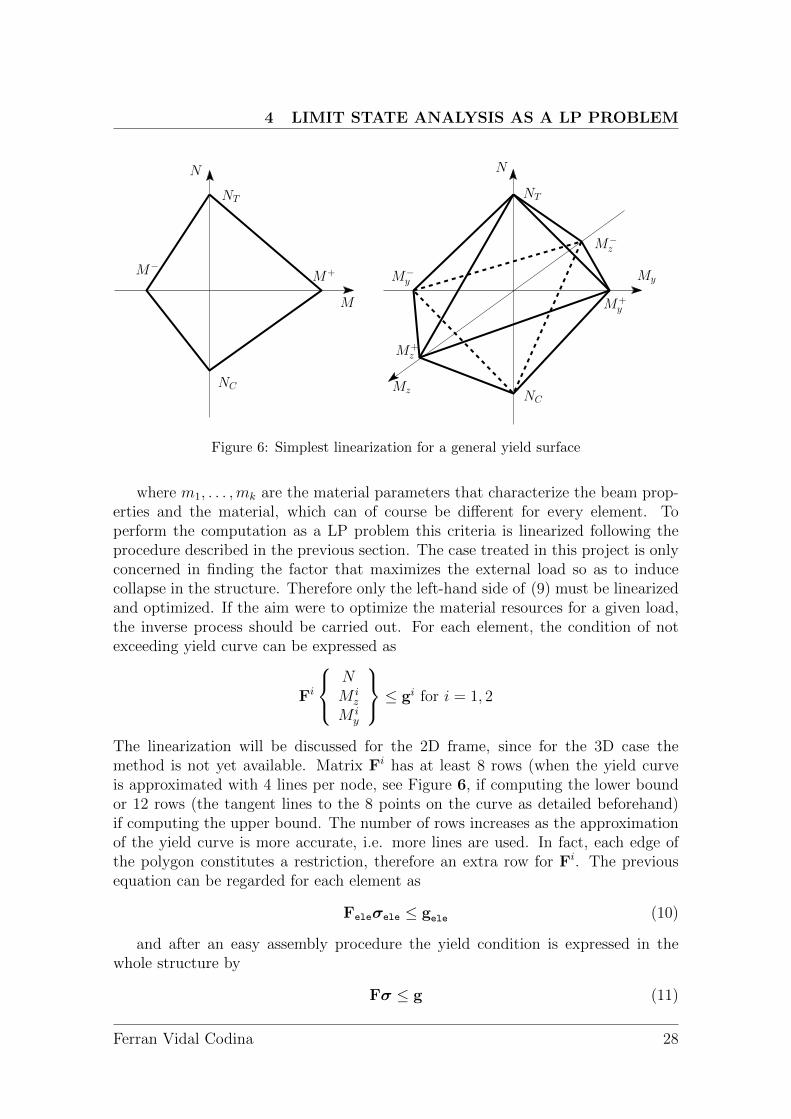
The linearization will be discussed for the 2D frame, since for the 3D case themethod is not yet available. Matrix Fi has at least 8 rows (when the yield curveis approximated with 4 lines per node, see Figure 6, if computing the lower boundor 12 rows (the tangent lines to the 8 points on the curve as detailed beforehand)if computing the upper bound. The number of rows increases as the approximationof the yield curve is more accurate, i.e. more lines are used. In fact, each edge ofthe polygon constitutes a restriction, therefore an extra row for Fi. The previousequation can be regarded for each element as
Feleσele ≤ gele (10)
and after an easy assembly procedure the yield condition is expressed in thewhole structure by
Fσ ≤ g (11)
Ferran Vidal Codina 28
4 LIMIT STATE ANALYSIS AS A LP PROBLEM
The number of columns of F equals the total number of generalized stress pa-rameters, i.e. the dimension of σ, 3nel. The number of rows is at least twice (onefor each node of each element) the number of structure elements times the numberof lines used to approximate the yield curve, minimum 4/6 per node, depending onthe bound that is being computed. From now on, a subscript will be used in orderto differentiate among the upper and the lower bound. Hence, the number of rowsof FLB is minimum 8nel, while the number of rows of FUB is at least 12nel It shouldbe noted that if a nodal point is a junction of several bars, yield at this node will bechecked as many times as the number of bars that join at the node. Thus if plasticflow is reached at a a node information about which bar contributes to the plasticattainment can be obtained.
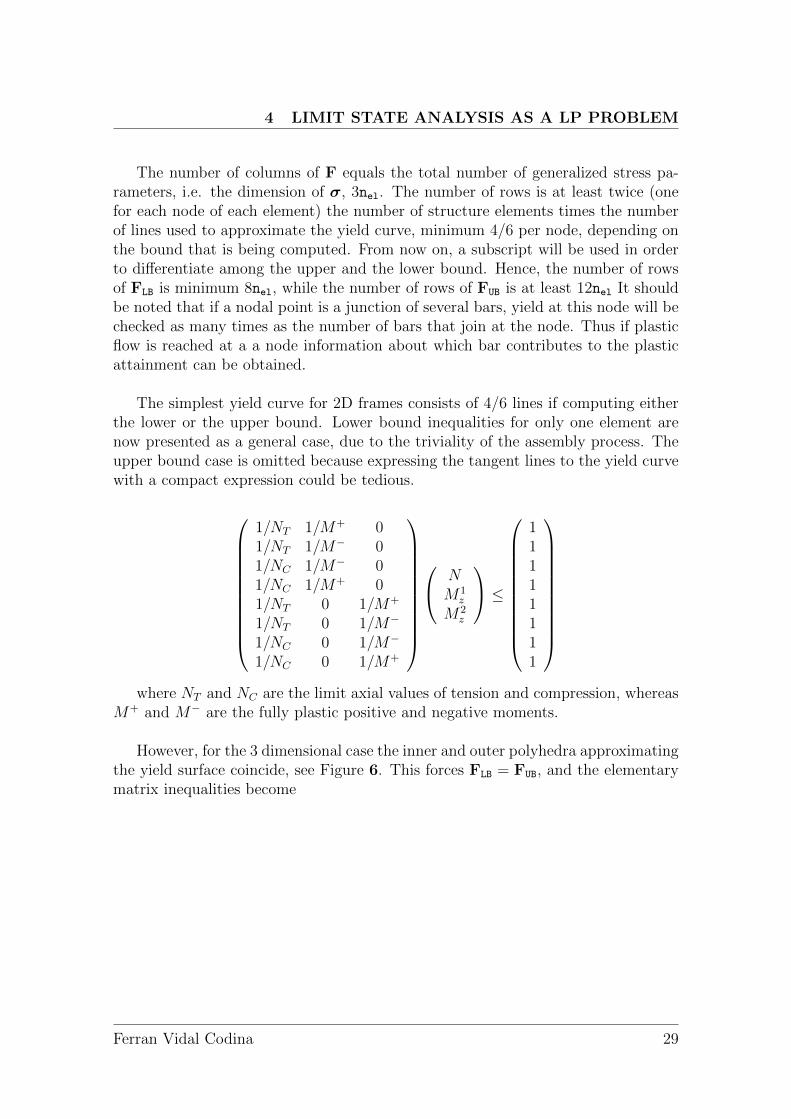
The simplest yield curve for 2D frames consists of 4/6 lines if computing eitherthe lower or the upper bound. Lower bound inequalities for only one element arenow presented as a general case, due to the triviality of the assembly process. Theupper bound case is omitted because expressing the tangent lines to the yield curvewith a compact expression could be tedious.
1/NT 1/M+ 01/NT 1/M− 01/NC 1/M− 01/NC 1/M+ 01/NT 0 1/M+
1/NT 0 1/M−
1/NC 0 1/M−
1/NC 0 1/M+
NM1
z
M2z
≤
11111111
where NT and NC are the limit axial values of tension and compression, whereas
M+ and M− are the fully plastic positive and negative moments.
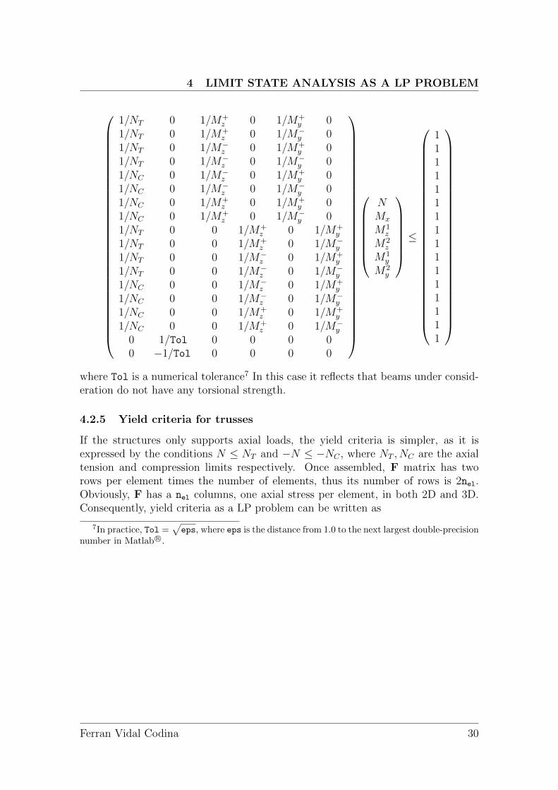
However, for the 3 dimensional case the inner and outer polyhedra approximatingthe yield surface coincide, see Figure 6. This forces FLB = FUB, and the elementarymatrix inequalities become
Ferran Vidal Codina 29
4 LIMIT STATE ANALYSIS AS A LP PROBLEM
1/NT 0 1/M+z 0 1/M+
y 01/NT 0 1/M+
z 0 1/M−y 0
1/NT 0 1/M−z 0 1/M+
y 01/NT 0 1/M−
z 0 1/M−y 0
1/NC 0 1/M−z 0 1/M+
y 01/NC 0 1/M−
z 0 1/M−y 0
1/NC 0 1/M+z 0 1/M+
y 01/NC 0 1/M+
z 0 1/M−y 0
1/NT 0 0 1/M+z 0 1/M+
y
1/NT 0 0 1/M+z 0 1/M−
y
1/NT 0 0 1/M−z 0 1/M+
y
1/NT 0 0 1/M−z 0 1/M−
y
1/NC 0 0 1/M−z 0 1/M+
y
1/NC 0 0 1/M−z 0 1/M−
y
1/NC 0 0 1/M+z 0 1/M+
y
1/NC 0 0 1/M+z 0 1/M−
y
0 1/Tol 0 0 0 00 −1/Tol 0 0 0 0
NMx
M1z
M2z
M1y
M2y
≤
1111111111111111
where Tol is a numerical tolerance7 In this case it reflects that beams under consid-eration do not have any torsional strength.
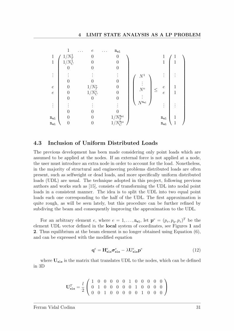
4.2.5 Yield criteria for trusses
If the structures only supports axial loads, the yield criteria is simpler, as it isexpressed by the conditions N ≤ NT and −N ≤ −NC , where NT , NC are the axialtension and compression limits respectively. Once assembled, F matrix has tworows per element times the number of elements, thus its number of rows is 2nel.Obviously, F has a nel columns, one axial stress per element, in both 2D and 3D.Consequently, yield criteria as a LP problem can be written as
7In practice, Tol =√eps, where eps is the distance from 1.0 to the next largest double-precision
number in Matlab R©.
Ferran Vidal Codina 30
4 LIMIT STATE ANALYSIS AS A LP PROBLEM
1 . . . e . . . nel1 1/N1
T 0 01 1/N1
C 0 00 0 0
......
......
0 0 0e 0 1/N e
T 0e 0 1/N e
C 00 0 0
......
......
0 0 0nel 0 0 1/Nnel
T
nel 0 0 1/NnelC
N1
...N e
...Nnel
≤
1 11 1
......
e 1e 1
......
nel 1nel 1
4.3 Inclusion of Uniform Distributed Loads
The previous development has been made considering only point loads which areassumed to be applied at the nodes. If an external force is not applied at a node,the user must introduce an extra node in order to account for the load. Nonetheless,in the majority of structural and engineering problems distributed loads are oftenpresent, such as selfweight or dead loads, and more specifically uniform distributedloads (UDL) are usual. The technique adopted in this project, following previousauthors and works such as [15], consists of transforming the UDL into nodal pointloads in a consistent manner. The idea is to split the UDL into two equal pointloads each one corresponding to the half of the UDL. The first approximation isquite rough, as will be seen lately, but this procedure can be further refined bysubdiving the beam and consequently improving the approximation to the UDL.
For an arbitrary element e, where e = 1, . . . , nel, let pe = (px, py, pz)T be the
element UDL vector defined in the local system of coordinates, see Figures 1 and2. Thus equilibrium at the beam element is no longer obtained using Equation (6),and can be expressed with the modified equation
qe = Heeleσ
eele − λUe
elepe (12)
where Uele is the matrix that translates UDL to the nodes, which can be definedin 3D
UTele =
l
2
1 0 0 0 0 0 1 0 0 0 0 00 1 0 0 0 0 0 1 0 0 0 00 0 1 0 0 0 0 0 1 0 0 0
Ferran Vidal Codina 31
4 LIMIT STATE ANALYSIS AS A LP PROBLEM
where l is the beam element length. It should be pointed out that UDL is alsoamplified by the sought load factor λ. Since the element equilibrium equation ismodified, so is the global equilibrium equation (8). The definitive equation that willbe provided to the LP solver will be the following
Hσ = Gr + λf (13)
with the definition of f as the force vector, which contemplates both nodal andUDL loads, namely f = f + Up. In this latter expression, pT = (pT
1 , . . . ,pTnel
)
and UT =(
U1eleT
1T. . . UeleT
nelT)
where T is the rotation matrix defined
in (4.1.2). The software will automatically set either f or Up to the zero matrixwhenever a matrix of point loads or UDL respectively is not detected.
SecantTangentMoment distribution Max moment
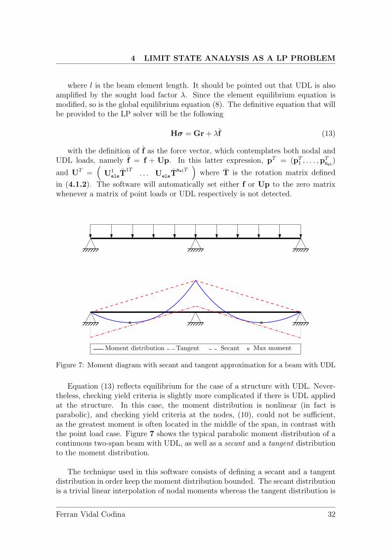
Figure 7: Moment diagram with secant and tangent approximation for a beam with UDL
Equation (13) reflects equilibrium for the case of a structure with UDL. Never-theless, checking yield criteria is slightly more complicated if there is UDL appliedat the structure. In this case, the moment distribution is nonlinear (in fact isparabolic), and checking yield criteria at the nodes, (10), could not be sufficient,as the greatest moment is often located in the middle of the span, in contrast withthe point load case. Figure 7 shows the typical parabolic moment distribution of acontinuous two-span beam with UDL, as well as a secant and a tangent distributionto the moment distribution.
The technique used in this software consists of defining a secant and a tangentdistribution in order keep the moment distribution bounded. The secant distributionis a trivial linear interpolation of nodal moments whereas the tangent distribution is
Ferran Vidal Codina 32
4 LIMIT STATE ANALYSIS AS A LP PROBLEM
the secant distribution translated a quantity of pil2
8, i = y, z depending on the axis
that supports load, as can be observed in Figure 7. These two approximations of themoment diagram induce an upper bound and a lower bound on the exact collapsefactor, which nature is completely different from the yield curve approximation, butboth can be complemented.
If only the secant distribution is considered, yield inequalities contained in (11)will lead to an upper bound of the exact collapse factor. Since yield conditionsare only checked at the nodes, if yield is attained at the element nodes the secantmoment distribution produces a factor that coincides with the exact one. However,if yield occurs somewhere on the span, the secant load factor will be always greaterthan the actual one.
On the other hand, if the LP problem is computed including the both the secantand the tangent moment distribution, a lower bound can be obtained. Obviously,adding more inequalities to (11) can only decrease λ. Moreover, since the exactmoment distribution always lies in between the secant and the moment, checkingyield criteria at the nodes will always produce a worse case scenario. For thispurpose, the generalized element stress vector for an arbitrary element e, σe
ele must
be modified according to the pil2
8, i = y, z translation when accounting the tangent
distribution
σeele = σe
ele − λΣeele ⇐⇒ σe
ele =
NMx
M1z
M2z
M1y
M2y
− λ
00
peyl2
8
peyl2
8
pezl2
8
pezl2
8
Thus, equation (10) transforms into
Feleσele ≤ gele ⇐⇒ Fele(σele − λΣele) ≤ gele ⇐⇒ Feleσele ≤ gele + λFeleΣele
by naming gele = FeleΣele we obtain the expression for the tangent distribution.Obviously, if no UDL is present gele = 0. The assembly process is trivial, and thematrices for the whole structure are easily obtained. The compact form that will beused in the LP problem is reached by considering both the secant and the tangentdistribution in the same equation, i.e.(
FF
)σ − λ
(0g
)≤(
gg
)Ferran Vidal Codina 33
4 LIMIT STATE ANALYSIS AS A LP PROBLEM
Finally, it is important to recall that if the UDL has a component along thex-direction of the local coordinate system the axial forces must be modified accord-ingly at corresponding equations in (10) (one for each node). This approach alwaysproduce an upper and lower bound of the load factor and this for any subdivision ofthe elements bearing UDL. Moreover, since the distance between the secant and the
tangent moment distributions is pil2
8with i either y or z depending on the flexural
axis considered, the bound gap decreases quadratically, obviously with the squareof the subdivision length.
4.3.1 Combination of yield and UDL bounding
When computing the collapse load factor via the LP problem, two different ap-proaches have been proposed that induce lower and upper bounds to the exact loadfactor. The approximation of the yield curve using an inscribed polygon producesa lower bound and the circumscribed polygon an upper bound. On the other hand,and considering UDL on the structure, using a secant distribution to the momentdiagram leads to an upper bound of the load factor, whereas using both the secantand the tangent distribution a lower bound is obtained.
If loading on the structure consists only of external point loads, bounding ofthe load factor is origined only by the approximation of the yield curve. However,the most common case in structural calculus involves UDL, and thus it must beconsidered. In order to obtain consistent bounds on the exact collapse load factor,the Lower Bound will be the one obtained by using an inscribed polygon to theyield curve and the secant and tangent distribution to the moment diagram. Con-sequently, the Upper Bound is computed by approximating the yield curve with acircumscribed polygon and the moment distribution using the secant interpolation.Thereby, this procedure ensures that the Upper Bound is always greater than theLower Bound, and therefore the bound gap (BG), which is the difference betweenthe UB and the LB, is positive.
Recall that the latter refers to 2D frames, since bounding for 3D frames is onlyaccomplished via the secant and the tangent moment distribution, as the yield sur-face is approximated inwards and outwards using the simplest linearization in Figure6.
4.4 The LP problem
For the general case of a structure with both point loads and UDL, and once equi-librium and yield conditions are defined, the optimization problem can be writtenas
Ferran Vidal Codina 34
4 LIMIT STATE ANALYSIS AS A LP PROBLEM
maximize λ
subject to Hσ = Gr + λf (14)
FUBσ ≤ gUB
if the aim is to obtain the UB or
maximize λ
subject to Hσ = Gr + λf
FLBσ ≤ gLB (15)
FLBσ − λg ≤ gLB
if computing the LB. In these formulations, λ ∈ R, σ ∈ R6nel and r ∈ Rngr
are unknown variables (ngr is the number of geometric restrictions), whereas H ∈R6nnp×6nel , G ∈ R6nnp×ngr , f ∈ R6nnp , FLB ∈ R18nel×6nel , FUB ∈ R18nel×6nel , gLB ∈ R18nel ,gUB ∈ R16nel and g ∈ R16nel are given data. On this latter five the number of rows isa minimum, since improving the approximation of the yield surface provides moreequations, hence more rows are added to the matrix. As has been commented, thisimplementation for 3D frames is not yet available, but it is for 2D frames. Note thatalthough λ ∈ R, the solutions of the LP problem always imply that the collapse loadis nonnegative. The proof of this fact is that taking λ = 0 there exists a feasiblestress state (σ0, r0) that verifies equilibrium and such that yield is not attained atany node, i.e. Hσ0 = Gr0 and Fσ0 ≤ g which can be (σ0, r0) = (0, 0). Sincethe problem is a maximization over λ, nonnegativity is thereby guaranteed. Forexpressing the LP problem in the general form described by (4) it will be clearlydifferentiated the LB and UB computation, as well as its dual problem.
4.4.1 Upper Bound
Auxiliary variables will be used in order to write the LP problem in the compactform. Using the following definitions
cT = (−1, 0, . . . , 0), xT = (λ,σT , rT ),
D =( 1 6nel ngr
18nel 0 FUB 0)
, e = gUB,
A =( 1 6nel ngr
6nnp f −H G), b = 0,
problem (14) is equivalent to (4). As a direct consequence, its dual problemshould be equivalent to (5), which expressed in the structural notation states as
Ferran Vidal Codina 35
4 LIMIT STATE ANALYSIS AS A LP PROBLEM
minimize gTUBη
subject to fTν = 1
GTν = 0 (16)
FTUBη = HTν
η ≥ 0
where the first restriction is a normalization of the work produced by external
forces. This term, fTν = 1 involves external forces, both nodal and UDL, and the
generalized displacement rates ν. Consequently, if external work is equalized to theinternal dissipation, that is
λfTν = gT
UBη (17)
this latter equation shows that the objective function of the dual problem for anykinematically admissible solution is the load factor λ found using the kinematic the-orem, as it must be according to [10].
For dimensional criteria, the dual variables η, ν belong to [R+]18nel and R6nnp .Moreover, the latter is clearly associated to the displacement rate and angular veloc-ity of each node of the structure. Due to it, it is easy to observe that the restrictionGTν = 0 imposes the geometric restrictions. The other dual variable, η, is a vectorof nonnegative plastic multiplier rates. At optimality, only the active constraints ofthe primal problem associated with plastic failure will have its corresponding pos-itive plastic multiplier rate. Thus gT
UBη is the plastic dissipation of internal work.Finally, the third constraint, FT
UBη = HTν, imposes compatibility.
4.4.2 Lower Bound
The same notation is used, although variables here are slightly different
cT = (−1, 0, . . . , 0), xT = (λ,σT , rT ),
D =
( 1 6nel ngr18nel 0 FLB 018nel −g FLB 0
), e =
(gLB
gLB
),
A =( 1 6nel ngr
6nnp f −H G), b = 0
This development supposes that UDL loads are present in the structure, whichis the most general case. If not, the last row of D and e must be suppressed, andthe rename that is now proposed need not to be taken into account. Therefore, ifthe structure bears UDL loads, in order to obtain the dual problem, the elements ofthe D matrix are renamed in a more compact form
Ferran Vidal Codina 36
4 LIMIT STATE ANALYSIS AS A LP PROBLEM
FLB =
(FLB
FLB
), gLB =
(gLB
gLB
), g =
(0g
)With this new notation, the dual problem is written
minimize gTLBη
subject to fTν − gTη = 1
GTν = 0 (18)
FTLBη = HTν
η ≥ 0
Obviously, η ∈ [R+]36nel and ν ∈ R6nnp .
4.4.3 Problem normalization
Both problems (14) and (15) are not normalized. The inequalities that represent theyield conditions, see (11), are pseudo-normalized, as the right-hand-side is alwaysa vector of ones, whereas the equilibrium equation (13) is not normalized. Nor-malization and scaling of the problem may be important to convergence of the LPproblem and thus it gains interest. However, it should be noted that any scalingin the external load vector f has a direct effect not only in λ, but also in the dualvariables η and ν.
In the software both the external load vector and the vector g, which containsthe UDL, are scaled with the norm of f, before calling the LP solver. After theoptimization the variables affected and the external load vector are rescaled in orderto obtain the actual values.
4.4.4 Evaluation of the bound gap
In sections (4.2.4) and (4.3) two different approaches are detailed in order to boundthe exact collapse load factor. In the first one, the gap is arbitrarily reduced as thenumber of lines to approximate the yield curve at each node is increased, while inthe second the gap decreases quadratically as beam elements are split into halves.In order to determine an adaptive strategy to reduce the bound gap, which is oneof the further goals of the software, it is required to state the contribution of everyelement to the total gap.
Using both equations (17) and the dual problem (16) an upper bound of the loadfactor at collapse is simply
λUB = gTUBηUB = ηT
UBgUB (19)
Ferran Vidal Codina 37
5 USE OF STRUCTURAL COLLAPSE SIMULATOR
To determine a lower bound of the load factor the equilibrium equation (13)must be used, namely
HσLB = GrLB + λLBf
A lower bound of the collapse factor can be obtained right multiplying the ex-
pression before by νUB. Since νUB verifies the normalization restriction, fTν = 1, and
the geometric condition GTν = 0, the lower bound becomes λLB = νTUBHσLB, and
applying compatibility, i.e. the third restriction of the dual problem (16)
λLB = ηTUBFUBσLB (20)
The expressions for an upper bound (19) and a lower bound (20) determine thebound gap of the structure
∆ = λUB − λLB = ηTUB(gUB − FUBσLB)
which determine the accuracy of the computations. Regard that the secondconstraint of (14) and the positiveness of η imply that the bound gap is nonnegative.This latter expression is for the bound gap of the global structure. However, if anadaptive process is sought, information about the contribution of every element isrequired. This contribution can easily be determined, namely
∆ =∑e
∆e with ∆e = ηeUB,ele
T (geUB,ele − FUB,eleσ
eLB,ele),
where ∆e ≥ 0 as ηeUB,ele ≥ 0 by definition and ge
UB,ele − FUB,eleσeLB,ele ≥ 0 as it is
stated in (10).
5 Use of Structural Collapse Simulator
Once the problem has been studied and its formulation as a LP problem has beenwritten, it is highly interesting to detail how the Structural Collapse Simulator (SCS)is designed and how it can be employed by the user in order to obtain the collapseload factor for the desired structure. Firstly, it should be stated that the softwareutilized for developing the SCS is Matlab R©, as it provides an easy treatment ofmatrices and some efficient LP solvers. The program is designed with a descendentstructure and the main operations can be summarised as data input, data process-ing, creation of matrices, LP solver and postprocessing. The central commandingprogram that the user will work on the most is named main. From this file the userdecides which structure to compute and the postprocessing desired. It also accountsfor the time taken for the computation, and it is displayed on the screen. Furtherreferences will be made to main as the whole procedure is detailed.
Ferran Vidal Codina 38
5 USE OF STRUCTURAL COLLAPSE SIMULATOR
5.1 Data input
The data input is done via the so-called drivers, the programs that contain themain information about the structure that is about to be computed. For everynew structure, the user will be asked to create a new driver, with different infor-mation but with the same exact development, and therefore it is crucial to regard it.
5.1.1 Logicals for structure characterization
Firstly, two boolean must be defined, and are initially set to zero. The first boolean,istruss, states whereas the computation will be made for a framed or for a trussedstructure. If the second boolean, isnorm, is activated, no approximation of the yieldcurve is carried out. Consequently, the yield curve is described with 4 lines per node,see Figure 6, for both the lower and the upper bound, which is exactly the yieldcheck that is recommended in the steel normative. This is the most conservativeapproach to the yield curve, but it is sometimes useful in order to determine theinfluence of the UDL in the bound gap, since is the only condition that preventsboth the lower and the upper bound from coinciding.
5.1.2 Nodal and Connectivity matrices
Once known which kind of structure will be computed and how to make the yieldcurve computation, geometric data must be provided. The nodal matrix X ∈Rnnp×nsd, with nsd being the number of spatial dimensions, 2 or 3, must be en-tered with each row referring to a node, with the x, y and z coordinates as the first,second and third column. Node numeration will automatically be assigned by theSCS according to the node’s row number in the X matrix.
The connectivity matrix T is defined as a Matlab R© cell array. The first cell isa real-valued matrix belonging to Rnel×3, which will be named T1. In the first andthe second column of the T1 matrix the beginning and the end nodes of the beamelement must be introduced, according to the coordinate system defined in Figure1. As happened before, the elements numeration depends on how the T1 matrixis constructed . In the third column the number of lines to approximate the yieldcurve8 of each node in the element is detailed. This number must be a multiple of4, and can be different for each element. It should be regarded that this number isuseless in case the isnorm is set to 1, which is the case for 3D frames.
The second cell, T2, is a string array, with as many columns as the number ofelements nel. Each column contains a string that indicates the cross section of each
8This number will be used for the inscribed polygon, and the circumscribed polygon will consistof essentially the same number of lines plus the extra restrictions detailed in (4.2.3), which willbe regarded afterwards.
Ferran Vidal Codina 39
5 USE OF STRUCTURAL COLLAPSE SIMULATOR
element for the further check of the yield curve. There exists the option of plottingthe structure to reassure the introduction of nodal and connectivity data has beensuccessful, by using the function PlotStructure in the driver. When computing a 3Dframe an additional cell T3 must be entered, which contains the direction of the webvector for every beam in the global coordinate system.
5.1.3 External Load matrices
Furthermore, load conditions must be entered by the user. Since both point loadsand UDL are accounted, load data may concern either one or two matrices. Thematrix of external point loads, namely P, contains an undetermined number or rows.This latter is due to the fact that the P needs not to have an entrance for every node,but only for the nodes with point loads. Hence, it will have as many rows as thenumber of nodes carrying external forces, namely 1 ≤ # ≤ nnp. This implies thatthe user is not asked to fill the matrix with 0s for the non-loaded nodes, which issensible accounting the dimension of the problems that will be solved. The numberof columns and the data contained in them varies in each case, namely
� nsd = 2 istruss = 0 P = (node, Px, Py,Mz)nsd = 2 istruss = 1 P = (node, Px, Py)
� nsd = 3 istruss = 0 P = (node, Px, Py, Pz,Mx,My,Mz)nsd = 3 istruss = 1 P = (node, Px, Py, Pz)
The forces must be referred to a global coordinate system, which must be definedby the user prior to SCS computations, as X, T and P matrices highly depend on it.According to the global coordinate system, signs must be placed correctly, and ingeneral considering counter-clockwise moments to be positive.
The matrix that carries the UDL loads will normally be named UDL, and similarlyto P will have no stipulated number of rows. In fact, this matrix has as many rowsas the number of elements with UDL, thus 1 ≤ # ≤ nel . Regarding the columns,the cases now are
� nsd = 2 istruss = 0 UDL = (element, px, py)
� nsd = 3 istruss = 0 UDL = (element, px, py, pz)
The loads are defined using local coordinate system defined in Figure 1.
5.1.4 Geometric Restrictions matrix
Finally, geometric restrictions such as embeddings or simple supports need to beintroduced. This will be done using the C matrix, with ngr rows and 3k columns,with k ≥ 1. With the moving index i = 0, . . . , k − 1, for every row column 3i + 1
Ferran Vidal Codina 40
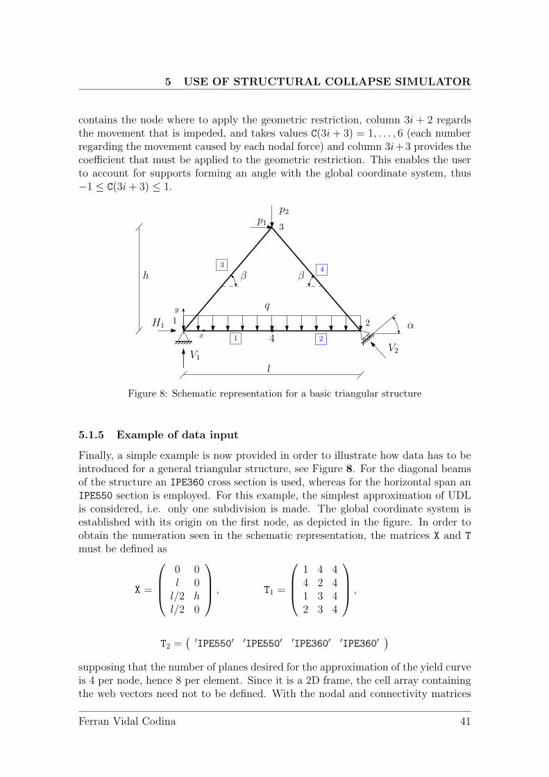
5 USE OF STRUCTURAL COLLAPSE SIMULATOR
contains the node where to apply the geometric restriction, column 3i + 2 regardsthe movement that is impeded, and takes values C(3i + 3) = 1, . . . , 6 (each numberregarding the movement caused by each nodal force) and column 3i+3 provides thecoefficient that must be applied to the geometric restriction. This enables the userto account for supports forming an angle with the global coordinate system, thus−1 ≤ C(3i+ 3) ≤ 1.
α1 2
3
y
x
h
l
p1
q
21
β β
4
43
p2
V1
H1
V2
Figure 8: Schematic representation for a basic triangular structure
5.1.5 Example of data input
Finally, a simple example is now provided in order to illustrate how data has to beintroduced for a general triangular structure, see Figure 8. For the diagonal beamsof the structure an IPE360 cross section is used, whereas for the horizontal span anIPE550 section is employed. For this example, the simplest approximation of UDLis considered, i.e. only one subdivision is made. The global coordinate system isestablished with its origin on the first node, as depicted in the figure. In order toobtain the numeration seen in the schematic representation, the matrices X and T
must be defined as
X =
0 0l 0l/2 hl/2 0
, T1 =
1 4 44 2 41 3 42 3 4
,
T2 =( ′IPE550′ ′IPE550′ ′IPE360′ ′IPE360′
)supposing that the number of planes desired for the approximation of the yield curveis 4 per node, hence 8 per element. Since it is a 2D frame, the cell array containingthe web vectors need not to be defined. With the nodal and connectivity matrices
Ferran Vidal Codina 41
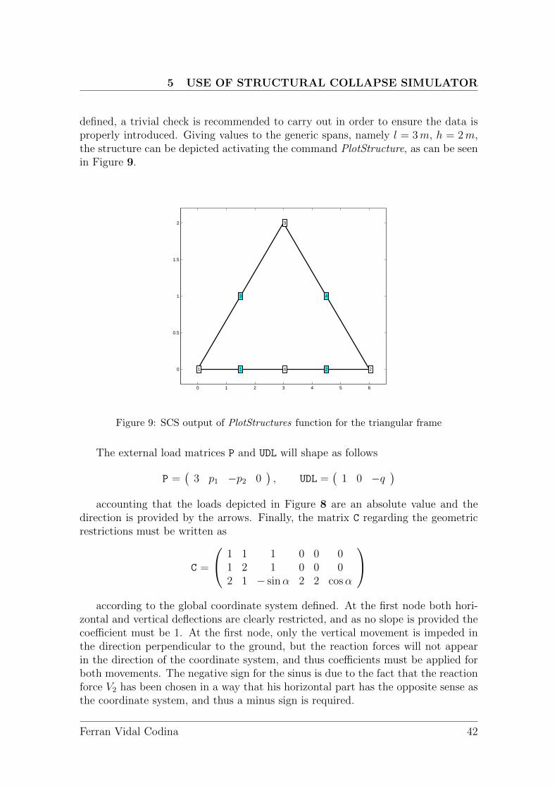
5 USE OF STRUCTURAL COLLAPSE SIMULATOR
defined, a trivial check is recommended to carry out in order to ensure the data isproperly introduced. Giving values to the generic spans, namely l = 3m, h = 2m,the structure can be depicted activating the command PlotStructure, as can be seenin Figure 9.
0 1 2 3 4 5 6
0
0.5
1
1.5
2
1 2
3
41 2
3 4
Figure 9: SCS output of PlotStructures function for the triangular frame
The external load matrices P and UDL will shape as follows
P =(
3 p1 −p2 0), UDL =
(1 0 −q
)accounting that the loads depicted in Figure 8 are an absolute value and the
direction is provided by the arrows. Finally, the matrix C regarding the geometricrestrictions must be written as
C =
1 1 1 0 0 01 2 1 0 0 02 1 − sinα 2 2 cosα
according to the global coordinate system defined. At the first node both hori-
zontal and vertical deflections are clearly restricted, and as no slope is provided thecoefficient must be 1. At the first node, only the vertical movement is impeded inthe direction perpendicular to the ground, but the reaction forces will not appearin the direction of the coordinate system, and thus coefficients must be applied forboth movements. The negative sign for the sinus is due to the fact that the reactionforce V2 has been chosen in a way that his horizontal part has the opposite sense asthe coordinate system, and thus a minus sign is required.
Ferran Vidal Codina 42
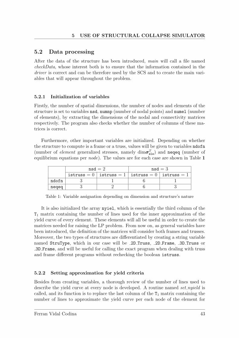
5 USE OF STRUCTURAL COLLAPSE SIMULATOR
5.2 Data processing
After the data of the structure has been introduced, main will call a file namedcheckData, whose interest both is to ensure that the information contained in thedriver is correct and can be therefore used by the SCS and to create the main vari-ables that will appear throughout the problem.
5.2.1 Initialization of variables
Firstly, the number of spatial dimensions, the number of nodes and elements of thestructure is set to variables nsd, numnp (number of nodal points) and numel (numberof elements), by extracting the dimensions of the nodal and connectivity matricesrespectively. The program also checks whether the number of columns of these ma-trices is correct.
Furthermore, other important variables are initialized. Depending on whetherthe structure to compute is a frame or a truss, values will be given to variables ndofn(number of element generalized stresses, namely dimσT
ele) and neqeq (number ofequilibrium equations per node). The values are for each case are shown in Table 1
nsd = 2 nsd = 3istruss = 0 istruss = 1 istruss = 0 istruss = 1
ndofn 3 1 6 1neqeq 3 2 6 3
Table 1: Variable assignation depending on dimension and structure’s nature
It is also initialized the array nyiel, which is essentially the third column of theT1 matrix containing the number of lines used for the inner approximation of theyield curve of every element. These elements will all be useful in order to create thematrices needed for raising the LP problem. From now on, as general variables havebeen introduced, the definition of the matrices will consider both frames and trusses.Moreover, the two types of structures are differentiated by creating a string variablenamed StruType, which in our case will be 2D Truss, 2D Frame, 3D Truss or3D Frame, and will be useful for calling the exact program when dealing with truss
and frame different programs without rechecking the boolean istruss.
5.2.2 Setting approximation for yield criteria
Besides from creating variables, a thorough review of the number of lines used todescribe the yield curve at every node is developed. A routine named set nyield iscalled, and its function is to replace the last column of the T1 matrix containing thenumber of lines to approximate the yield curve per each node of the element for
Ferran Vidal Codina 43
5 USE OF STRUCTURAL COLLAPSE SIMULATOR
the total lines that will be used per element for the lower bound9. In general, thisnumber will be multiplied by 2, since the lines for an element is twice the lines fora single node.
However, this function is significant in two special cases: where the normativecriteria is applied, i.e. isnorm is set to 1, or where some or all cross sections ofelements are classified as C4. As seen in (4.2.1), these sections do not attain plasticflow, and thus it is preposterous to propose a the yield curve approximation, andyield will be checked using the simplest approximation in Figure 6, just as if norma-tive criteria was applied. In order to work with C4 sections, the user must explicitlyadd it to the name of the cross section in the T2 string array, using notation ’ C4’at the end of the cross section name. When working with normative criteria, thefunction set nyield will set the whole third column of the T1 matrix automatically toeither 18 planes or 8 lines per element, depending on the dimension of the structure.On the other hand, if the computation is carried without normative criteria (only2D case can be computed this way so far) but some or all of beam elements areexpected to behave as a C410, the function will set the corresponding number ofplanes to 8, it does not have to be necessarily every element of the structure.
5.2.3 Dimensional check
Finally, checkData is relevant as it confirms whether the data for the P, UDL and C isproperly introduced. Besides checking that the number of columns of the matricesare appropriate, it creates either an empty P or UDL matrix in case only UDL loadsor point loads are considered respectively. Moreover, it displays an error if the useris trying to compute a trussed structure with UDL loads, stopping the execution ofthe SCS.
5.3 Creation of matrices
Once the data provided has proven to be correct, the SCS advances to create andassemble the matrices needed for setting the LP problem, namely H, f, G and allthe matrices involved in the yield criteria, for upper and lower bound calculations.This is done via the program Create var, which is addressed from the main file. Theprogram creates the matrices one-by-one and stores them in the workspace, readyto be used by the LP solver.
9The upper bound is properly treated based on the lower bound information and the extrarestrictions
10Class types of different cross sections ought to be known in advance by consulting catalogues.For instance, IPE and HEB sections are usually C1, sometimes C2. For further information, Arcelor-Mittal catalogues can be checked out.
Ferran Vidal Codina 44
5 USE OF STRUCTURAL COLLAPSE SIMULATOR
5.3.1 Equilibrium matrices
The construction of the H ∈ Rneqeq∗numnp×numel∗ndofn matrix, which is done in thefunction CreateH, will no further be discussed, as both the rotation and the assem-bly process has been widely detailed in (4.1.5). In order to obtain f = f + Up, thetwo independent matrices are firstly generated. The creation of f, which consistsof only point loads, is as simple as reshaping the input matrix P into a columnarray of neqeq ∗ numnp rows, since for each node horizontal, vertical and momentloads are placed in this order, and can be done by calling Createf. The procedurefor generating the Up has been discussed in (4.3), and also a neqeq ∗ numnp × 1array is obtained after rotation, assembly and reshaping process in CreateUp hasfinished. Once the sum is made, the euclidean norm of f is stored as Scale in orderto normalize the LP problem as seen in (4.4.3) The geometric restriction matrixG ∈ Rneqeq∗numnp×numgr is obtained after properly reshaping the C matrix in order thateach geometric restriction relates to the corresponding node and element, and thefunction responsible for it is CreateG.
5.3.2 Yield criteria matrices
Once equilibrium matrices are stored, yield criteria matrices must be generated,namely FUB, FLB, gUB, gLB and g. A routine named CreateFg is used for creatingthese latter matrices. The g arrays are the simplest, as consists only of a vector ofones. The amount of restrictions used to make an inner approximation the yieldcurve for every node of every element, which are the number of rows of gLB, can befound by summing the elements of nyiel, that is sum nyiel. The number of rows ofgUB is essentially the number of rows of gLB plus the extra restrictions. As explainedin (4.2.4), when dealing with a double I/H-shaped section the extra restrictions are2 per node, i.e. 4 per element. Nevertheless, extra restrictions must be checked atevery element since C4 cross section beams obviously do not have extra restrictions.The total amount of extra restrictions is a temporary variable named extra rest.Of course, if is isnorm=1 no extra restrictions are used. Hence, gLB ∈ Rsum nyiel×1
and gUB ∈ R(sum nyiel+extra rest)×1. Note that yield criteria for trusses has alreadybeen specified in (4.2.5). The following developments are only for 2D frames, since3D frames are computed using normative criteria and the matrices are the ones de-fined in Section (4.2.4).
According to the latter, the dimensions of the F matrices are easily determined,namely FUB ∈ R(sum nyiel+extra rest)×numel∗ndofn and FLB ∈ Rsum nyiel×numel∗ndofn. Thecoefficients of the two matrices are found by calling the function Create Fgele 2D Framefor each element. For each element the function returns the elementary matrix thatappears in (4.2.4) if isnorm=1 or the cross section is a C4. If none of this condi-tions happens, then another function named yield Ishape 2D11 is accessed in order
11So far yield has only been studied for I/H-shaped cross sections.
Ferran Vidal Codina 45
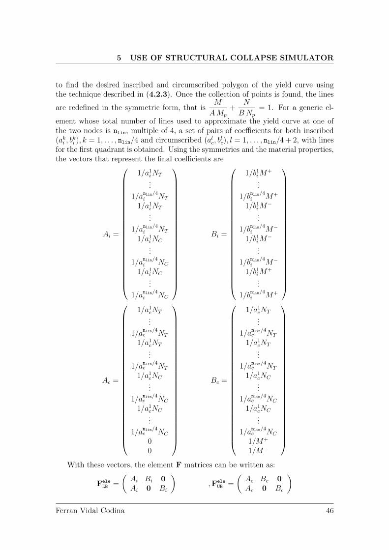
5 USE OF STRUCTURAL COLLAPSE SIMULATOR
to find the desired inscribed and circumscribed polygon of the yield curve usingthe technique described in (4.2.3). Once the collection of points is found, the lines
are redefined in the symmetric form, that isM
AMp
+N
BNp
= 1. For a generic el-
ement whose total number of lines used to approximate the yield curve at one ofthe two nodes is nlin, multiple of 4, a set of pairs of coefficients for both inscribed(aki , b
ki ), k = 1, . . . , nlin/4 and circumscribed (alc, b
lc), l = 1, . . . , nlin/4 + 2, with lines
for the first quadrant is obtained. Using the symmetries and the material properties,the vectors that represent the final coefficients are
Ai =
1/a1iNT...
1/anlin/4i NT
1/a1iNT...
1/anlin/4i NT
1/a1iNC...
1/anlin/4i NC
1/a1iNC...
1/anlin/4i NC
Bi =
1/b1iM+
...
1/bnlin/4i M+
1/b1iM−
...
1/bnlin/4i M−
1/b1iM−
...
1/bnlin/4i M−
1/b1iM+
...
1/bnlin/4i M+
Ac =
1/a1cNT...
1/anlin/4c NT
1/a1cNT...
1/anlin/4c NT
1/a1cNC...
1/anlin/4c NC
1/a1cNC...
1/anlin/4c NC
00
Bc =
1/a1cNT...
1/anlin/4c NT
1/a1cNT...
1/anlin/4c NT
1/a1cNC...
1/anlin/4c NC
1/a1cNC...
1/anlin/4c NC
1/M+
1/M−
With these vectors, the element F matrices can be written as:
FeleLB =
(Ai Bi 0Ai 0 Bi
),Fele
UB =
(Ac Bc 0Ac 0 Bc
)
Ferran Vidal Codina 46
5 USE OF STRUCTURAL COLLAPSE SIMULATOR
Finally, the g ∈ Rsum nyiel×1 is obtained assembling the various gele. The con-struction of this latter vector, for a generic element of length l, differs slightly fromthe one seen in (4.3), since the external loads must be scaled in order to normalizethe problem. Thus, we obtain
gele =l2
8 ∗ ScaleFeleLB
(0 0 pey pey pez pez
)TOnce these matrices have been generated, before advancing to the LP solver,
SCS checks whether the structure is or not supporting UDL. If the problem beingcomputed bears UDL, the matrices for the lower bound computation are renamed asexplained in (4.4.2), and thus we will work with matrices FLB, gLB and g = (0 gT )T
for the lower bound. Note that it is advisable to state first the presence of UDL, asfor a point loaded structure this operation is useless and in fact only adds redundantequations to the LP problem.
5.4 LP Solver
The process of solving the LP problems involves first transforming the equilibriumand yield matrices for both lower and upper bounds problems into the adequatenotation, see (4.4.1) and (4.4.2). The function in where this rearrangement takesplace is named LP solver, and it is called twice from the main file. Placing thevariables in order to obtain the standard LP form is due to the fact that the solverthat has been employed for the SCS is Matlab R© linsolve. Although it is not themost efficient LP solver, it suffices for the structures computed. However, in thefuture the intention is to adapt the SCS to work with SDPT3 in order to enhancethe solving capacities.
For both problems, once the process of solving is successfully completed (al-lowing a maximum number of 500 iterations) the solution vector xT = (λ,σT , rT )and the Lagrange multipliers (η,ν) are obtained. The function also rescales λ, themultipliers in order to obtain the adequate information, which is properly storedfor postprocessing. Matrices g, f are rescaled as well, in order to recover the inputdata. Finally, the program verifies that the solution meets the hypotheses of thebasic approach to the limit analysis problem, i.e. equilibrium and yield is satisfiedeverywhere. In case not all restrictions are satisfied, the program details which equa-tions of either equilibrium or yield are violated, and thus enables an easy overcheck.
The default options include displaying λ and the result from the verification ofequilibrium and yield, either showing a positive message or the list of restrictionsthat are not satisfied for both equilibrium and yield. The bound gap ∆ will also bedisplayed.
Ferran Vidal Codina 47
5 USE OF STRUCTURAL COLLAPSE SIMULATOR
5.5 Postprocessing
SCS has been provided with several postprocessing tools in order not only to depictthe final outcome of the computation, but also to support the process of adequatelyunderstanding and analysing the results obtained, a basic task that users of SCSneed to be able to develop. Thus, postprocessing tools can be extremely usefulwhenever SCS provides weird or nonsense results, for both programmers and users.These tools all located on the main page, thereby it is trivial to deactivate them ifdesired. They are activated as a default setting.
5.5.1 Gap Evaluation
This option provides a numel×2 matrix named gap eval, in where the first columnshows the element contribution ∆e to the total bound gap ∆, and the second col-umn displays the number of element itself. The contribution is computed using theoperations discussed in (4.4.4) in a function named GapEvaluation, which utilizesthe output of the LP solver, and the result is shown using descending order, i.e. theelement with the greatest contribution occupies the first row.
This enables the user to form an average idea of which sections need more specificcalculations, namely using more lines to approximate the yield curve, subdividingthe beam element into more subelements or even both improvements. Generally,better computations can be made by manually adjusting these latter features ofthe structure in the driver, although the initial idea is to turn this procedure intoan adaptive one, which we believe it must be hand driven. This idea will be laterdiscussed.
5.5.2 Plotting plastic hinges and displacement rates
This is a tremendously useful tool to understand how framed structures react to theexternal loading and how the collapse mechanism looks like. Moreover, it can leadto detect mistakes in the implementation or even in the problem modeling. Theplastic hinges and displacements will be depicted only for the lower bound problem,as they represent a safe scenario and for structures with UDL the program will beable locate plastic hinges even though before subdividing the elements. The mainreason to explain this latter is that the lower bound for UDL seeks for the exactmoment distribution lying between the secant and the tangent distribution, andthus the combination of stresses that attain plastic flow can be in this range withno need to have a node defined. This helps detect plastic hinges in advance.
In C1, C2 type cross sections, a plastic hinge forms when the fully plastic mo-ment is attained at one node under pure bending stress. However, if compressionbending stresses take place, a plastic hinge develops if the yield curve is reachedat some point. The process of locating plastic hinges is developed in FindHinges.The physical condition to locate plastic hinges is to find the yield inequalities that
Ferran Vidal Codina 48

5 USE OF STRUCTURAL COLLAPSE SIMULATOR
turn to equalities. Mathematically, as it is expressed in FindHinges, the constraintswhere |gLB − FLBσLB + λLBg| < Tol.
The output of FindHinges is the matrix hinges, with three columns and asmany rows as plastic hinges. The first column represents the node that attains plas-tic flow, the second shows which element this node belongs to (recall that the samenode can belong to several elements as they intersect in the node, and yield must notnecessarily be reached at every one of these elements), and finally the third columnprovides information about what restriction of the node is violated. Using the samenotation as before, if the yield curve at a node is approximated using nlin lines,the restriction’s range is 1 to nlin, accounting the conventional counter-clockwisenumeration of quadrants.
The aforementioned information is used to plot both the plastic hinges and thedisplacement rates of the structures, which are represented by the dual variable ν.The program used to depict this data is PlotHinges, and provides both the basicrepresentation of the structure12, nodes and bars, and the structure at collapse, i.e.with the plastic hinges (red background and black number for the node) and thedisplacement rate in red arrows. Note that there is the possibility of scaling thedisplacement rates using an amplifying factor in order to be visible, since they areoften to small to be seen in the representation.
5.5.3 Plotting elements failure
Obviously, the concept of plastic hinges lacks sense when dealing with trussed struc-tures. For this reason the routine PlotFailure has been designed. When computinga truss, SCS will access this routine ignoring PlotHinges, employing the data ex-tracted in FindHinges. This easy program represents the structure depicting in redthe elements that fail due to traction and in blue the elements that fail for compres-sion. This routine also offers the option of plotting the deformed structure in thesame conditions as explained before.
5.5.4 Plotting bending moment diagram
Knowing the moment stress distribution is often a useful tool for either verifying ordenying the outcome of a computation. As explained before, the moment diagramwill be depicted only for the lower bound problem and for the 2D frame case.
The only information that will be used is the value of σLB. The representationis done by the function PlotMoments, and the procedure is as simple as unitingthe moment stresses for nodes in the same element with lines. This will lead toan accurate plot for point loaded structure, but it may be weird when computing
12The same that can be obtained by activating the option PlotStructure in the driver of eachstructure
Ferran Vidal Codina 49
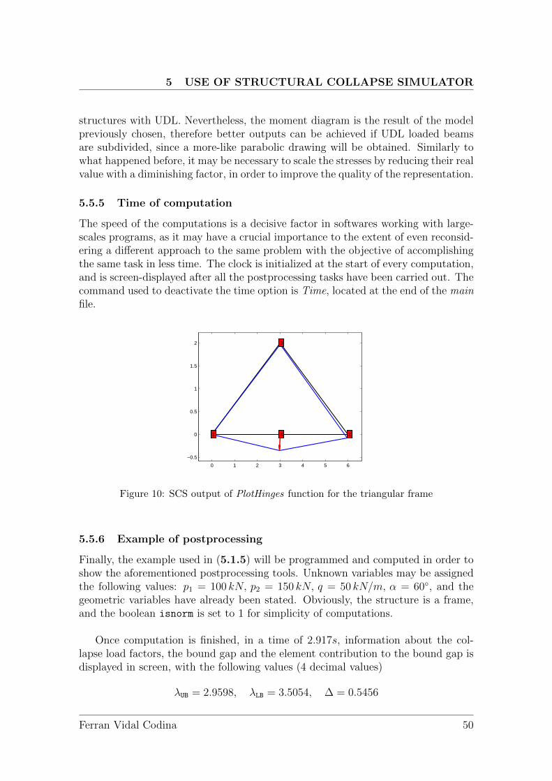
5 USE OF STRUCTURAL COLLAPSE SIMULATOR
structures with UDL. Nevertheless, the moment diagram is the result of the modelpreviously chosen, therefore better outputs can be achieved if UDL loaded beamsare subdivided, since a more-like parabolic drawing will be obtained. Similarly towhat happened before, it may be necessary to scale the stresses by reducing their realvalue with a diminishing factor, in order to improve the quality of the representation.
5.5.5 Time of computation
The speed of the computations is a decisive factor in softwares working with large-scales programs, as it may have a crucial importance to the extent of even reconsid-ering a different approach to the same problem with the objective of accomplishingthe same task in less time. The clock is initialized at the start of every computation,and is screen-displayed after all the postprocessing tasks have been carried out. Thecommand used to deactivate the time option is Time, located at the end of the mainfile.
0 1 2 3 4 5 6
−0.5
0
0.5
1
1.5
2
1 2
3
441 2
3
Figure 10: SCS output of PlotHinges function for the triangular frame
5.5.6 Example of postprocessing
Finally, the example used in (5.1.5) will be programmed and computed in order toshow the aforementioned postprocessing tools. Unknown variables may be assignedthe following values: p1 = 100 kN, p2 = 150 kN, q = 50 kN/m, α = 60◦, and thegeometric variables have already been stated. Obviously, the structure is a frame,and the boolean isnorm is set to 1 for simplicity of computations.
Once computation is finished, in a time of 2.917s, information about the col-lapse load factors, the bound gap and the element contribution to the bound gap isdisplayed in screen, with the following values (4 decimal values)
λUB = 2.9598, λLB = 3.5054, ∆ = 0.5456
Ferran Vidal Codina 50
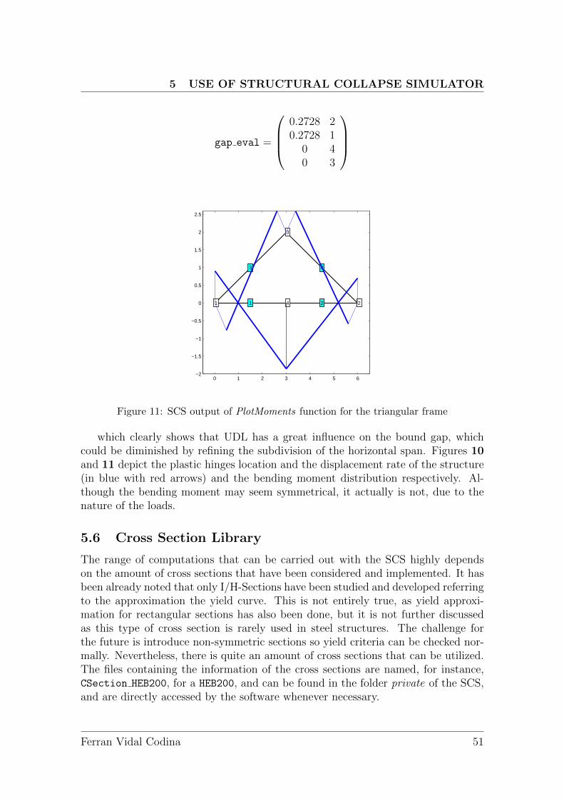
5 USE OF STRUCTURAL COLLAPSE SIMULATOR
gap eval =
0.2728 20.2728 1
0 40 3
0 1 2 3 4 5 6−2
−1.5
−1
−0.5
0
0.5
1
1.5
2
2.5
1 2
3
41 2
3 4
Figure 11: SCS output of PlotMoments function for the triangular frame
which clearly shows that UDL has a great influence on the bound gap, whichcould be diminished by refining the subdivision of the horizontal span. Figures 10and 11 depict the plastic hinges location and the displacement rate of the structure(in blue with red arrows) and the bending moment distribution respectively. Al-though the bending moment may seem symmetrical, it actually is not, due to thenature of the loads.
5.6 Cross Section Library
The range of computations that can be carried out with the SCS highly dependson the amount of cross sections that have been considered and implemented. It hasbeen already noted that only I/H-Sections have been studied and developed referringto the approximation the yield curve. This is not entirely true, as yield approxi-mation for rectangular sections has also been done, but it is not further discussedas this type of cross section is rarely used in steel structures. The challenge forthe future is introduce non-symmetric sections so yield criteria can be checked nor-mally. Nevertheless, there is quite an amount of cross sections that can be utilized.The files containing the information of the cross sections are named, for instance,CSection HEB200, for a HEB200, and can be found in the folder private of the SCS,and are directly accessed by the software whenever necessary.
Ferran Vidal Codina 51
5 USE OF STRUCTURAL COLLAPSE SIMULATOR
The library of cross sections will suppose that the steel employed has an elasticlimit of fy = 275 N/mm2 = 275000 kN/m2, (the subscript is for yield) i.e. a steelcharacterized as S275. By changing data in the files appropriately, the steel usedfor the structure can be S235, S355 or even S460 if structural, building or economicimplications must be met.
5.6.1 I/H-shaped
Obviously this is the most typical cross section employed for steel structures design,as it provides satisfying results for both economic and structural issues. The twoseries used in SCS so far are IPE and HEB. According to the catalogues these sec-tions attain plastic flow, C1 or C2, almost always. The only exceptions regard thehighest and widest sections under pure compression stress, when they cannot reachplastic regime. Since it is highly improbable to encounter pure compression stressessituations in actual structures, I/H-shaped structures will be considered to attainplastic flow.
The information that has to be provided to create a cross section file are both thegeometric data, namely tw, h, b, hw, A and the plastic data, i.e. NT , NC , M
+p , M
−p
which in this case the positive and negative stresses coincide. The geometric data isdirectly extracted from the catalogues, and the plastic data can be easily obtainedby performing the simple computations
NT = −NC = AfyM+
p = −M−p = Wpz fy
where Wpz is the plastic resistant modulus of the section around the strong axis,z, (remember Figure 3) and can be found in the catalogues. Regard that the unitsmainly used in the program are kN and m, and thus both the geometrical andplastic data have to be calculated consistently.
Nevertheless, it may not always be correct to evaluate this sections using plasticdata. Mostly, if the computations are desired to be made according to the elasticprinciples, plastic flow must not be attained. Again, it may respond to structural,safety or economical conditions, and therefore it must be considered. Setting isnorm
to 1 implies that elastic criteria is adopted, since the yield curve cannot be approx-imated. In the data processing stage, the detection of isnorm=1 automaticallyleads the program to add the string ’ NORM’ to the name of the file. This allowsSCS to recognize which file, CSection HEB200 or CSection HEB200 NORM (continu-ing with the aforementioned example), should be accessed, depending on whethercalculations will be made regarding plastic or elastic regime. The NORM files con-tain the same geometric data, but the plastic data is replaced with the elastic data,NT , NC , M
+e , M
−e . The elastic axial limit loads are the same as the plastic ones,
whereas the elastic bending moments are slightly different, and can be computed as
Ferran Vidal Codina 52

5 USE OF STRUCTURAL COLLAPSE SIMULATOR
M+e = −M−
e = Wez fy
where Wez is the elastic resistant modulus of the section around the axis z,and it can be obtained from the catalogues. Obviously, the elastic magnitudes aresignificantly lower than the plastic ones, and thus considering calculations with thenormative prescriptions will yield to lower collapse loads.
5.6.2 C4 Sections
SCS enables the users to introduce C4 sections that are not considered in the cat-alogues. These sections are usually used in plates or thin steel structures. It iscommon that slender or thin cross sections have a behavior that can be classified asC4. To enter a new cross section to the library, a file must be created and the nameof the section has to end with the string ’ C4’ to assure the program will recognizeit and consider it properly for the yield calculations. Moreover, only elastic datais required, since no computations will demand geometric data. It is advisable toprovide an approximate scheme of the section and the axis orientation in order toassist the user for further employments of the file. Finally, elastic data must beprovided, namely NT , NC , M
+e , M
−e , which can be obtained performing the latter
operations or by directly introducing the numerical value. This easy process widensthe horizons of the SCS, since a great deal of the production of steel industriesconsists of beams or plates with C4 cross sections.
5.7 Utility of SCS
Finally, before studying examples to show the functioning of SCS, its utility incomparison to other softwares must be highlighted. In engineering, the majorityof structures that have to be dealt with are hyperstatic structures, i.e. they arenot statically determined. It implies that structural collapse appears when severalsections attain plastic flow. Consequently, the structure turns into a mechanism,and the failure of the sections cause the structure to lose its stability and bear-ing capacities. Thereby, a given structure can continue to bear external load eventhough one or diverse plastic hinges have formed in sections where plastic limit hasbeen reached. Namely, the structure does not collapse until the necessary numberof plastic hinges to turn the structure into a mechanism have formed.
5.7.1 Linear analysis
Linear analysis, either analytical or by computer, only indicate the failure of thefirst section, regarding normative criteria, not the collapse of the entire structure.These methods are interesting for engineering since they are robust methods of com-putation, they provide reliable results, the cost of computation is reduced and theyalways yield to safe results.
Ferran Vidal Codina 53
6 NUMERICAL EXAMPLES
On the other hand, there are several drawbacks in linear analysis methods. Asthey detect only the failure of the first section, the actual collapse load is unknown,and therefore they lead to overdimensioning of the structure. Moreover, they donot provide neither information about the security margin nor how the collapsemechanism shapes. This latter impedes to work on improvements of the structure’sdesign. Finally, nonlinearity of the yield curve is not considered in the computations.Consequently, linear methods constitute a useful tool for having a first approach atthe structure but accuracy of results and data can be improved by using nonlinearmethods.
5.7.2 Nonlinear analysis
Nonlinear analysis considers the structure’s real behavior and the evolution of theexternal loading. Methods using nonlinear analysis are realistic, as they show the ac-tual changes the structure suffers. Furthermore, information can be obtained aboutthe actual collapse load and the collapse mechanism.
Although nonlinear analysis provides more accurate information for an engineer,it is not always advisable to use. In general, nonlinear analysis methods tend notto be robust, and thus require an expert user. They are unefficient methods, withelevated cost and time of computation, either for the definition of the problem or forthe computation. Besides from this, as a certain amount of initial data is requiredthe accuracy of the input data lessens, lowering the reliability of the method.
5.7.3 SCS
The Structural Collapse Simulator is a computational tool of numerical calculusspecifically designed for the robust, efficient and reliable evaluation of structures.SCS employs linear programming techniques to find the unique solution of the prob-lem, thus robustness is assured. Moreover, nonexpert users can easily perform com-putations with the SCS. It is clearly an efficient software, as its basis in LP enablesthe use of several optimization packages in order to improve the calculations. Finally,it constitutes a reliable method since it provides a bounded solution, indicating theminimum or safe value of the load factor (lower bound) and the precision of thecomputations (bound gap). The bounding can be reduced arbitrarily by the user.SCS satisfyingly combines the characteristics of the linear and the nonlinear analysismethods, achieving interesting results as can be seen in next section.
6 Numerical examples
6.1 Simply supported beam
The simply supported beam of one span subject to a uniform distributed load alongthe span is perhaps the simplest, yet one of the most useful examples to both show
Ferran Vidal Codina 54
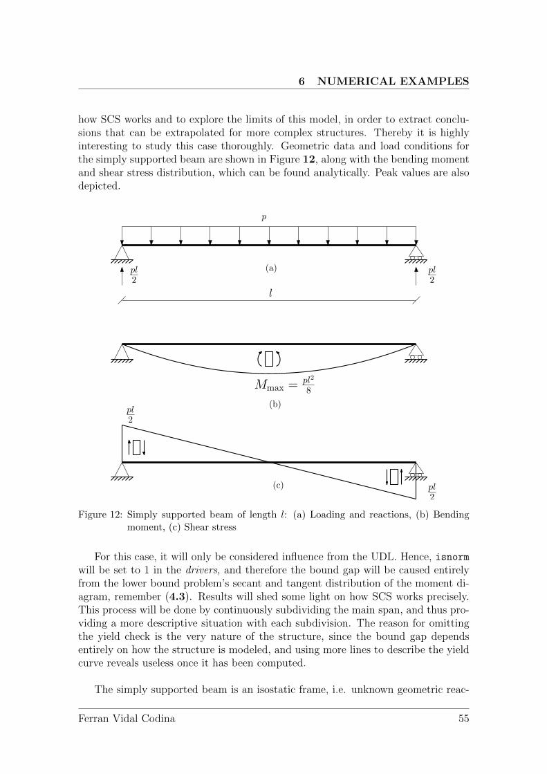
6 NUMERICAL EXAMPLES
how SCS works and to explore the limits of this model, in order to extract conclu-sions that can be extrapolated for more complex structures. Thereby it is highlyinteresting to study this case thoroughly. Geometric data and load conditions forthe simply supported beam are shown in Figure 12, along with the bending momentand shear stress distribution, which can be found analytically. Peak values are alsodepicted.
Mmax =pl2
8
p
pl2
pl2
pl2
pl2
(a)
(b)
(c)
l
Figure 12: Simply supported beam of length l: (a) Loading and reactions, (b) Bendingmoment, (c) Shear stress
For this case, it will only be considered influence from the UDL. Hence, isnormwill be set to 1 in the drivers, and therefore the bound gap will be caused entirelyfrom the lower bound problem’s secant and tangent distribution of the moment di-agram, remember (4.3). Results will shed some light on how SCS works precisely.This process will be done by continuously subdividing the main span, and thus pro-viding a more descriptive situation with each subdivision. The reason for omittingthe yield check is the very nature of the structure, since the bound gap dependsentirely on how the structure is modeled, and using more lines to describe the yieldcurve reveals useless once it has been computed.
The simply supported beam is an isostatic frame, i.e. unknown geometric reac-
Ferran Vidal Codina 55
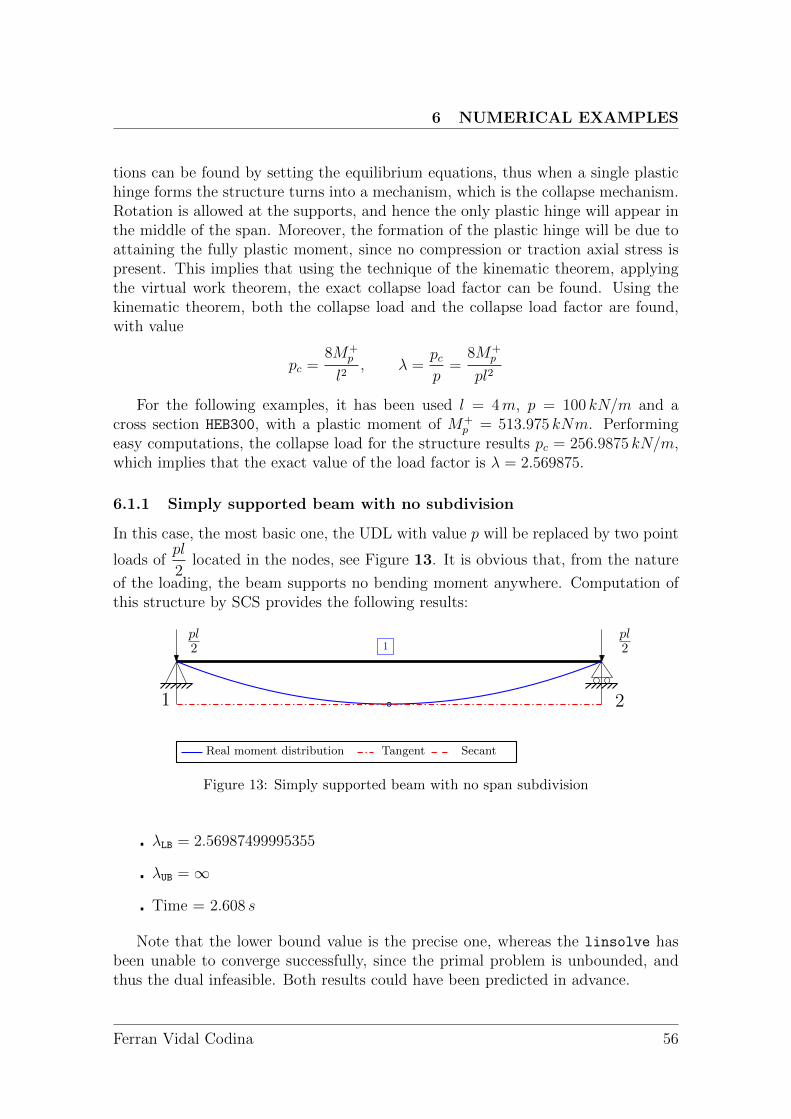
6 NUMERICAL EXAMPLES
tions can be found by setting the equilibrium equations, thus when a single plastichinge forms the structure turns into a mechanism, which is the collapse mechanism.Rotation is allowed at the supports, and hence the only plastic hinge will appear inthe middle of the span. Moreover, the formation of the plastic hinge will be due toattaining the fully plastic moment, since no compression or traction axial stress ispresent. This implies that using the technique of the kinematic theorem, applyingthe virtual work theorem, the exact collapse load factor can be found. Using thekinematic theorem, both the collapse load and the collapse load factor are found,with value
pc =8M+
p
l2, λ =
pcp
=8M+
p
pl2
For the following examples, it has been used l = 4m, p = 100 kN/m and across section HEB300, with a plastic moment of M+
p = 513.975 kNm. Performingeasy computations, the collapse load for the structure results pc = 256.9875 kN/m,which implies that the exact value of the load factor is λ = 2.569875.
6.1.1 Simply supported beam with no subdivision
In this case, the most basic one, the UDL with value p will be replaced by two point
loads ofpl
2located in the nodes, see Figure 13. It is obvious that, from the nature
of the loading, the beam supports no bending moment anywhere. Computation ofthis structure by SCS provides the following results:
pl2
pl21
1 2
SecantTangentReal moment distribution
Figure 13: Simply supported beam with no span subdivision
� λLB = 2.56987499995355
� λUB =∞
� Time = 2.608 s
Note that the lower bound value is the precise one, whereas the linsolve hasbeen unable to converge successfully, since the primal problem is unbounded, andthus the dual infeasible. Both results could have been predicted in advance.
Ferran Vidal Codina 56
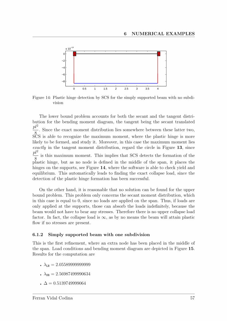
6 NUMERICAL EXAMPLES
0 0.5 1 1.5 2 2.5 3 3.5 4
−8
−6
−4
−2
0
x 10−14
11 22
Figure 14: Plastic hinge detection by SCS for the simply supported beam with no subdi-vision
The lower bound problem accounts for both the secant and the tangent distri-bution for the bending moment diagram, the tangent being the secant translatedpl2
8. Since the exact moment distribution lies somewhere between these latter two,
SCS is able to recognize the maximum moment, where the plastic hinge is morelikely to be formed, and study it. Moreover, in this case the maximum moment liesexactly in the tangent moment distribution, regard the circle in Figure 13, sincepl2
8is this maximum moment. This implies that SCS detects the formation of the
plastic hinge, but as no node is defined in the middle of the span, it places thehinges on the supports, see Figure 14, where the software is able to check yield andequilibrium. This automatically leads to finding the exact collapse load, since thedetection of the plastic hinge formation has been successful.
On the other hand, it is reasonable that no solution can be found for the upperbound problem. This problem only concerns the secant moment distribution, whichin this case is equal to 0, since no loads are applied on the span. Thus, if loads areonly applied at the supports, those can absorb the loads indefinitely, because thebeam would not have to bear any stresses. Therefore there is no upper collapse loadfactor. In fact, the collapse load is ∞, as by no means the beam will attain plasticflow if no stresses are present.
6.1.2 Simply supported beam with one subdivision
This is the first refinement, where an extra node has been placed in the middle ofthe span. Load conditions and bending moment diagram are depicted in Figure 15.Results for the computation are
� λLB = 2.05589999999999
� λUB = 2.56987499990634
� ∆ = 0.5139749999064
Ferran Vidal Codina 57
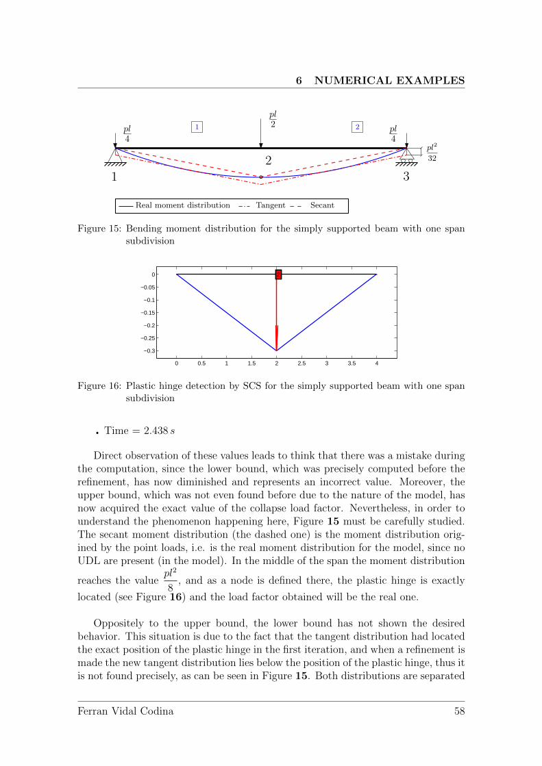
6 NUMERICAL EXAMPLES
pl4
pl4
pl2
12
3
1 2
SecantTangentReal moment distribution
pl2
32
Figure 15: Bending moment distribution for the simply supported beam with one spansubdivision
0 0.5 1 1.5 2 2.5 3 3.5 4
−0.3
−0.25
−0.2
−0.15
−0.1
−0.05
0 2222
Figure 16: Plastic hinge detection by SCS for the simply supported beam with one spansubdivision
� Time = 2.438 s
Direct observation of these values leads to think that there was a mistake duringthe computation, since the lower bound, which was precisely computed before therefinement, has now diminished and represents an incorrect value. Moreover, theupper bound, which was not even found before due to the nature of the model, hasnow acquired the exact value of the collapse load factor. Nevertheless, in order tounderstand the phenomenon happening here, Figure 15 must be carefully studied.The secant moment distribution (the dashed one) is the moment distribution orig-ined by the point loads, i.e. is the real moment distribution for the model, since noUDL are present (in the model). In the middle of the span the moment distribution
reaches the valuepl2
8, and as a node is defined there, the plastic hinge is exactly
located (see Figure 16) and the load factor obtained will be the real one.
Oppositely to the upper bound, the lower bound has not shown the desiredbehavior. This situation is due to the fact that the tangent distribution had locatedthe exact position of the plastic hinge in the first iteration, and when a refinement ismade the new tangent distribution lies below the position of the plastic hinge, thus itis not found precisely, as can be seen in Figure 15. Both distributions are separated
Ferran Vidal Codina 58
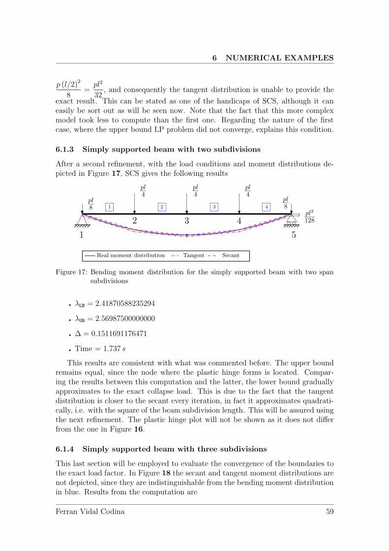
6 NUMERICAL EXAMPLES
p (l/2)2
8=pl2
32, and consequently the tangent distribution is unable to provide the
exact result. This can be stated as one of the handicaps of SCS, although it caneasily be sort out as will be seen now. Note that the fact that this more complexmodel took less to compute than the first one. Regarding the nature of the firstcase, where the upper bound LP problem did not converge, explains this condition.
6.1.3 Simply supported beam with two subdivisions
After a second refinement, with the load conditions and moment distributions de-picted in Figure 17, SCS gives the following results
pl8
pl8
pl4
1
2 3
1 2
SecantTangentReal moment distribution
pl4
pl4
3 4
4
5
pl2
128
Figure 17: Bending moment distribution for the simply supported beam with two spansubdivisions
� λLB = 2.41870588235294
� λUB = 2.56987500000000
� ∆ = 0.1511691176471
� Time = 1.737 s
This results are consistent with what was commented before. The upper boundremains equal, since the node where the plastic hinge forms is located. Compar-ing the results between this computation and the latter, the lower bound graduallyapproximates to the exact collapse load. This is due to the fact that the tangentdistribution is closer to the secant every iteration, in fact it approximates quadrati-cally, i.e. with the square of the beam subdivision length. This will be assured usingthe next refinement. The plastic hinge plot will not be shown as it does not differfrom the one in Figure 16.
6.1.4 Simply supported beam with three subdivisions
This last section will be employed to evaluate the convergence of the boundaries tothe exact load factor. In Figure 18 the secant and tangent moment distributions arenot depicted, since they are indistinguishable from the bending moment distributionin blue. Results from the computation are
Ferran Vidal Codina 59
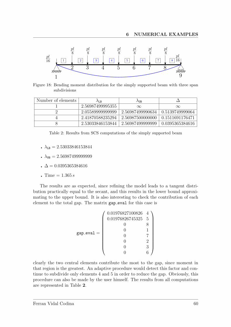
6 NUMERICAL EXAMPLES
pl16
pl16
1
2 3
1
pl8
pl8
4
pl8
pl8
pl8
pl8
pl8
2 3 4 5 6 7 8
5 6 7 8
9
Figure 18: Bending moment distribution for the simply supported beam with three spansubdivisions
Number of elements λLB λUB ∆1 2.56987499995355 ∞ ∞2 2.05589999999999 2.56987499990634 0.51397499990644 2.41870588235294 2.56987500000000 0.15116911764718 2.53033846153844 2.56987499999999 0.0395365384616
Table 2: Results from SCS computations of the simply supported beam
� λLB = 2.53033846153844
� λUB = 2.56987499999999
� ∆ = 0.0395365384616
� Time = 1.365 s
The results are as expected, since refining the model leads to a tangent distri-bution practically equal to the secant, and this results in the lower bound approxi-mating to the upper bound. It is also interesting to check the contribution of eachelement to the total gap. The matrix gap eval for this case is
gap eval =
0.01976827100826 40.01976826745325 5
0 80 10 70 20 30 6
clearly the two central elements contribute the most to the gap, since moment inthat region is the greatest. An adaptive procedure would detect this factor and con-tinue to subdivide only elements 4 and 5 in order to reduce the gap. Obviously, thisprocedure can also be made by the user himself. The results from all computationsare represented in Table 2.
Ferran Vidal Codina 60
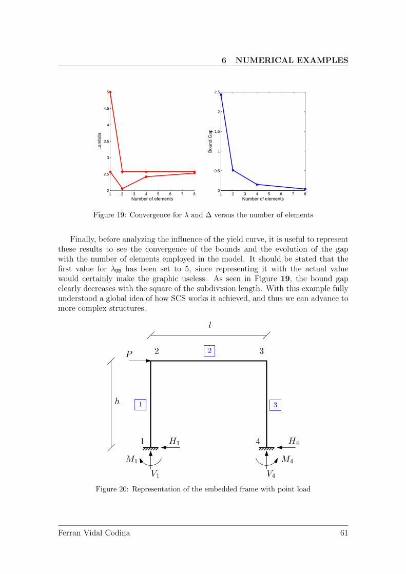
6 NUMERICAL EXAMPLES
1 2 3 4 5 6 7 82
2.5
3
3.5
4
4.5
5
Number of elements
Lam
bda
1 2 3 4 5 6 7 80
0.5
1
1.5
2
2.5
Number of elements
Bou
nd G
apFigure 19: Convergence for λ and ∆ versus the number of elements
Finally, before analyzing the influence of the yield curve, it is useful to representthese results to see the convergence of the bounds and the evolution of the gapwith the number of elements employed in the model. It should be stated that thefirst value for λUB has been set to 5, since representing it with the actual valuewould certainly make the graphic useless. As seen in Figure 19, the bound gapclearly decreases with the square of the subdivision length. With this example fullyunderstood a global idea of how SCS works it achieved, and thus we can advance tomore complex structures.
1
2
3
1
2 3
4
l
h
H1 H4
V1 V4
M4M1
P
Figure 20: Representation of the embedded frame with point load
Ferran Vidal Codina 61
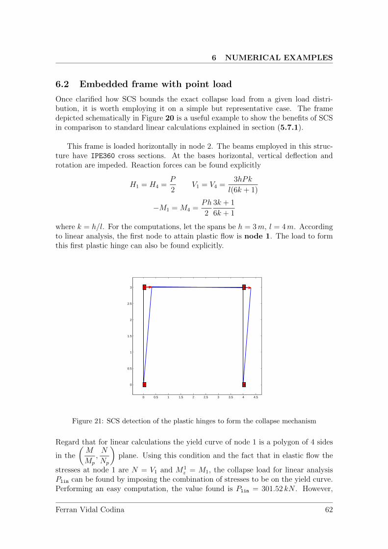
6 NUMERICAL EXAMPLES
6.2 Embedded frame with point load
Once clarified how SCS bounds the exact collapse load from a given load distri-bution, it is worth employing it on a simple but representative case. The framedepicted schematically in Figure 20 is a useful example to show the benefits of SCSin comparison to standard linear calculations explained in section (5.7.1).
This frame is loaded horizontally in node 2. The beams employed in this struc-ture have IPE360 cross sections. At the bases horizontal, vertical deflection androtation are impeded. Reaction forces can be found explicitly
H1 = H4 =P
2V1 = V4 =
3hPk
l(6k + 1)
−M1 = M4 =Ph
2
3k + 1
6k + 1
where k = h/l. For the computations, let the spans be h = 3m, l = 4m. Accordingto linear analysis, the first node to attain plastic flow is node 1. The load to formthis first plastic hinge can also be found explicitly.
0 0.5 1 1.5 2 2.5 3 3.5 4 4.5
0
0.5
1
1.5
2
2.5
3
1
2 3
4
Figure 21: SCS detection of the plastic hinges to form the collapse mechanism
Regard that for linear calculations the yield curve of node 1 is a polygon of 4 sides
in the
(M
Mp
,N
Np
)plane. Using this condition and the fact that in elastic flow the
stresses at node 1 are N = V1 and M1z = M1, the collapse load for linear analysis
Plin can be found by imposing the combination of stresses to be on the yield curve.Performing an easy computation, the value found is Plin = 301.52 kN . However,
Ferran Vidal Codina 62
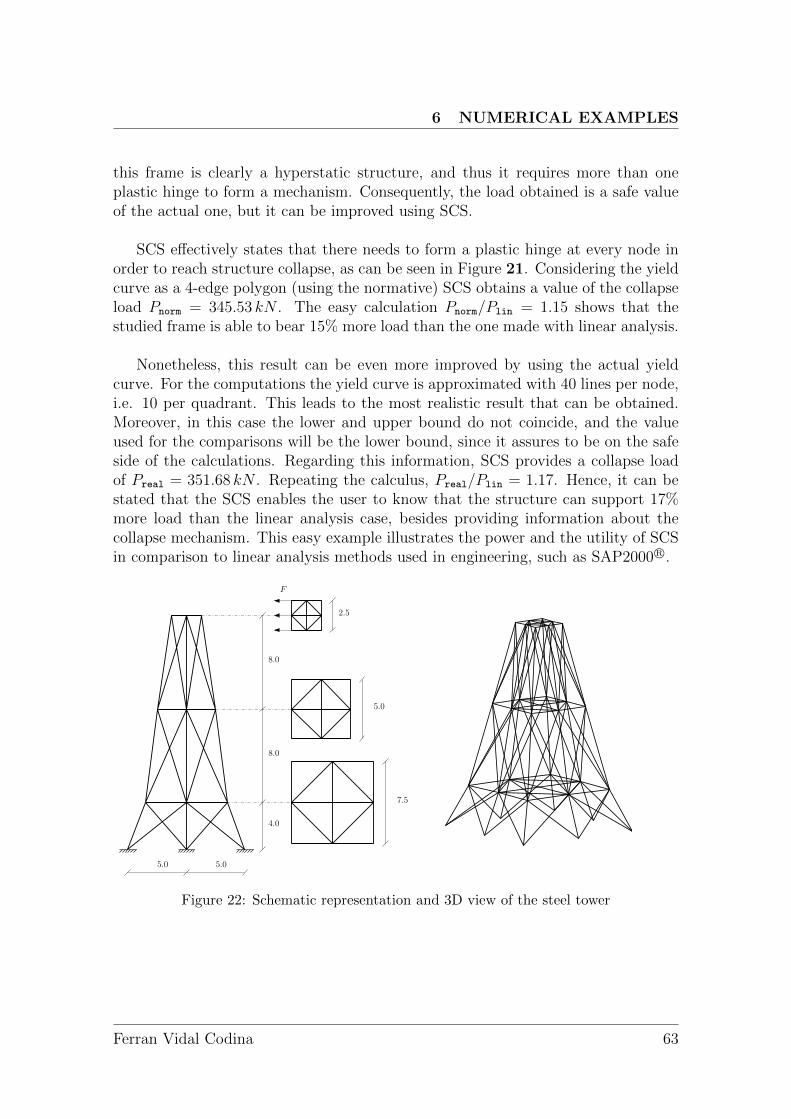
6 NUMERICAL EXAMPLES
this frame is clearly a hyperstatic structure, and thus it requires more than oneplastic hinge to form a mechanism. Consequently, the load obtained is a safe valueof the actual one, but it can be improved using SCS.
SCS effectively states that there needs to form a plastic hinge at every node inorder to reach structure collapse, as can be seen in Figure 21. Considering the yieldcurve as a 4-edge polygon (using the normative) SCS obtains a value of the collapseload Pnorm = 345.53 kN . The easy calculation Pnorm/Plin = 1.15 shows that thestudied frame is able to bear 15% more load than the one made with linear analysis.
Nonetheless, this result can be even more improved by using the actual yieldcurve. For the computations the yield curve is approximated with 40 lines per node,i.e. 10 per quadrant. This leads to the most realistic result that can be obtained.Moreover, in this case the lower and upper bound do not coincide, and the valueused for the comparisons will be the lower bound, since it assures to be on the safeside of the calculations. Regarding this information, SCS provides a collapse loadof Preal = 351.68 kN . Repeating the calculus, Preal/Plin = 1.17. Hence, it can bestated that the SCS enables the user to know that the structure can support 17%more load than the linear analysis case, besides providing information about thecollapse mechanism. This easy example illustrates the power and the utility of SCSin comparison to linear analysis methods used in engineering, such as SAP2000 R©.
5.0 5.0
4.0
8.0
8.0
2.5
5.0
7.5
F
Figure 22: Schematic representation and 3D view of the steel tower
Ferran Vidal Codina 63
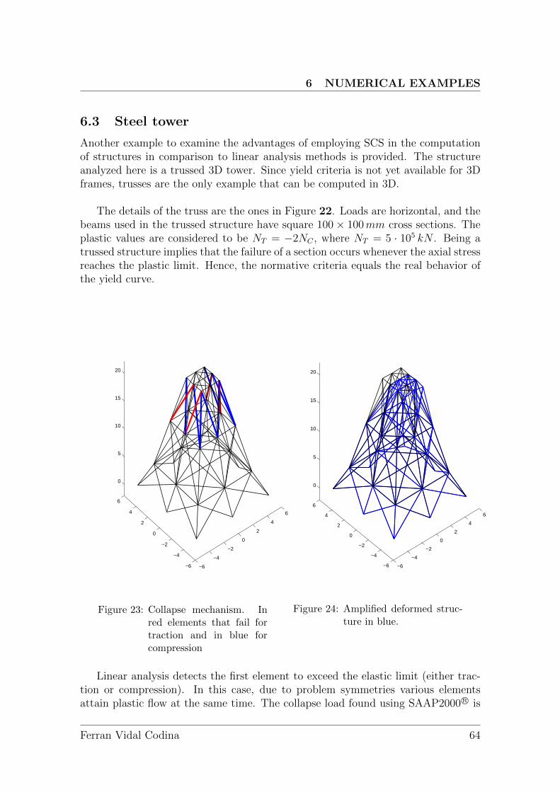
6 NUMERICAL EXAMPLES
6.3 Steel tower
Another example to examine the advantages of employing SCS in the computationof structures in comparison to linear analysis methods is provided. The structureanalyzed here is a trussed 3D tower. Since yield criteria is not yet available for 3Dframes, trusses are the only example that can be computed in 3D.
The details of the truss are the ones in Figure 22. Loads are horizontal, and thebeams used in the trussed structure have square 100× 100mm cross sections. Theplastic values are considered to be NT = −2NC , where NT = 5 · 105 kN . Being atrussed structure implies that the failure of a section occurs whenever the axial stressreaches the plastic limit. Hence, the normative criteria equals the real behavior ofthe yield curve.
−6
−4
−2
0
2
4
6
−6
−4
−2
0
2
4
6
0
5
10
15
20
Figure 23: Collapse mechanism. Inred elements that fail fortraction and in blue forcompression
−6
−4
−2
0
2
4
6
−6
−4
−2
0
2
4
6
0
5
10
15
20
Figure 24: Amplified deformed struc-ture in blue.
Linear analysis detects the first element to exceed the elastic limit (either trac-tion or compression). In this case, due to problem symmetries various elementsattain plastic flow at the same time. The collapse load found using SAAP2000 R© is
Ferran Vidal Codina 64
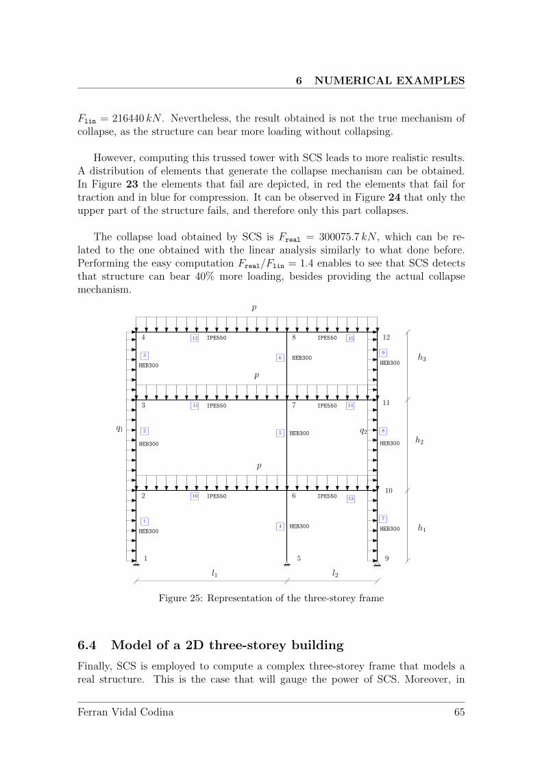
6 NUMERICAL EXAMPLES
Flin = 216440 kN . Nevertheless, the result obtained is not the true mechanism ofcollapse, as the structure can bear more loading without collapsing.
However, computing this trussed tower with SCS leads to more realistic results.A distribution of elements that generate the collapse mechanism can be obtained.In Figure 23 the elements that fail are depicted, in red the elements that fail fortraction and in blue for compression. It can be observed in Figure 24 that only theupper part of the structure fails, and therefore only this part collapses.
The collapse load obtained by SCS is Freal = 300075.7 kN , which can be re-lated to the one obtained with the linear analysis similarly to what done before.Performing the easy computation Freal/Flin = 1.4 enables to see that SCS detectsthat structure can bear 40% more loading, besides providing the actual collapsemechanism.
IPE550
IPE550
IPE550
IPE550
IPE550
IPE550
HEB300
HEB300
HEB300
HEB300
HEB300
HEB300
HEB300
HEB300
HEB300
l1 l2
p
p
p
q1 q2
h1
h2
h3
1
2
3
4
5
6
7
8
9
10
11
12
1
2
4
6
7
8
10
11
12 15
3
5
9
14
13
Figure 25: Representation of the three-storey frame
6.4 Model of a 2D three-storey building
Finally, SCS is employed to compute a complex three-storey frame that models areal structure. This is the case that will gauge the power of SCS. Moreover, in
Ferran Vidal Codina 65
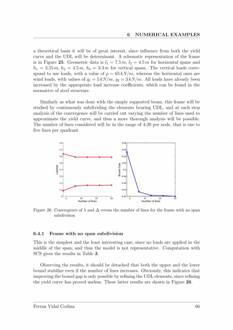
6 NUMERICAL EXAMPLES
a theoretical basis it will be of great interest, since influence from both the yieldcurve and the UDL will be determinant. A schematic representation of the frameis in Figure 25. Geometric data is l1 = 7.5m, l2 = 4.5m for horizontal spans andh1 = 3.55m, h2 = 4.5m, h3 = 3.3m for vertical spans. The vertical loads corre-spond to use loads, with a value of p = 65 kN/m, whereas the horizontal ones arewind loads, with values of q1 = 5 kN/m, q2 = 3 kN/m. All loads have already beenincreased by the appropriate load increase coefficients, which can be found in thenormative of steel structure.
Similarly as what was done with the simply supported beam, this frame will bestudied by continuously subdividing the elements bearing UDL, and at each stepanalysis of the convergence will be carried out varying the number of lines used toapproximate the yield curve, and thus a more thorough analysis will be possible.The number of lines considered will be in the range of 4-20 per node, that is one tofive lines per quadrant.
5 10 15 202
2.1
2.2
2.3
2.4
2.5
2.6
2.7
2.8
Number of lines
Lam
bda
5 10 15 200.42
0.44
0.46
0.48
0.5
0.52
0.54
0.56
0.58
Number of lines
Bou
nd G
ap
Figure 26: Convergence of λ and ∆ versus the number of lines for the frame with no spansubdivision
6.4.1 Frame with no span subdivision
This is the simplest and the least interesting case, since no loads are applied in themiddle of the span, and thus the model is not representative. Computation withSCS gives the results in Table 3.
Observing the results, it should be detached that both the upper and the lowerbound stabilize even if the number of lines increases. Obviously, this indicates thatimproving the bound gap is only possible by refining the UDL elements, since refiningthe yield curve has proved useless. These latter results are shown in Figure 26.
Ferran Vidal Codina 66
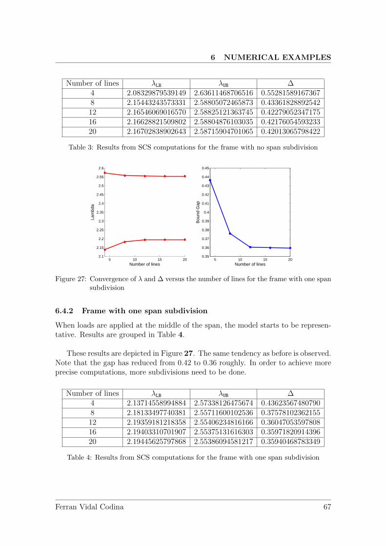
6 NUMERICAL EXAMPLES
Number of lines λLB λUB ∆4 2.08329879539149 2.63611468706516 0.552815891673678 2.15443243573331 2.58805072465873 0.4336182889254212 2.16546069016570 2.58825121363745 0.4227905234717516 2.16628821509802 2.58804876103035 0.4217605459323320 2.16702838902643 2.58715904701065 0.42013065798422
Table 3: Results from SCS computations for the frame with no span subdivision
5 10 15 202.1
2.15
2.2
2.25
2.3
2.35
2.4
2.45
2.5
2.55
2.6
Number of lines
Lam
bda
5 10 15 200.35
0.36
0.37
0.38
0.39
0.4
0.41
0.42
0.43
0.44
0.45
Number of lines
Bou
nd G
ap
Figure 27: Convergence of λ and ∆ versus the number of lines for the frame with one spansubdivision
6.4.2 Frame with one span subdivision
When loads are applied at the middle of the span, the model starts to be represen-tative. Results are grouped in Table 4.
These results are depicted in Figure 27. The same tendency as before is observed.Note that the gap has reduced from 0.42 to 0.36 roughly. In order to achieve moreprecise computations, more subdivisions need to be done.
Number of lines λLB λUB ∆4 2.13714558994884 2.57338126475674 0.436235674807908 2.18133497740381 2.55711600102536 0.3757810236215512 2.19359181218358 2.55406234816166 0.3604705359780816 2.19403310701907 2.55375131616303 0.3597182091439620 2.19445625797868 2.55386094581217 0.35940468783349
Table 4: Results from SCS computations for the frame with one span subdivision
Ferran Vidal Codina 67
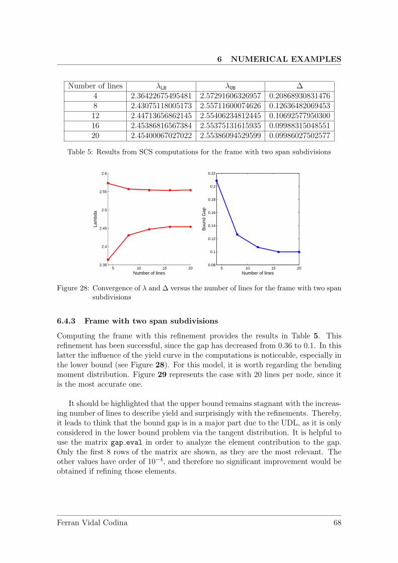
6 NUMERICAL EXAMPLES
Number of lines λLB λUB ∆4 2.36422675495481 2.57291606326957 0.208689308314768 2.43075118005173 2.55711600074626 0.1263648206945312 2.44713656862145 2.55406234812445 0.1069257795030016 2.45386816567384 2.55375131615935 0.0998831504855120 2.45400067027022 2.55386094529599 0.09986027502577
Table 5: Results from SCS computations for the frame with two span subdivisions
5 10 15 202.35
2.4
2.45
2.5
2.55
2.6
Number of lines
Lam
bda
5 10 15 200.08
0.1
0.12
0.14
0.16
0.18
0.2
0.22
Number of lines
Bou
nd G
ap
Figure 28: Convergence of λ and ∆ versus the number of lines for the frame with two spansubdivisions
6.4.3 Frame with two span subdivisions
Computing the frame with this refinement provides the results in Table 5. Thisrefinement has been successful, since the gap has decreased from 0.36 to 0.1. In thislatter the influence of the yield curve in the computations is noticeable, especially inthe lower bound (see Figure 28). For this model, it is worth regarding the bendingmoment distribution. Figure 29 represents the case with 20 lines per node, since itis the most accurate one.
It should be highlighted that the upper bound remains stagnant with the increas-ing number of lines to describe yield and surprisingly with the refinements. Thereby,it leads to think that the bound gap is in a major part due to the UDL, as it is onlyconsidered in the lower bound problem via the tangent distribution. It is helpful touse the matrix gap eval in order to analyze the element contribution to the gap.Only the first 8 rows of the matrix are shown, as they are the most relevant. Theother values have order of 10−4, and therefore no significant improvement would beobtained if refining those elements.
Ferran Vidal Codina 68
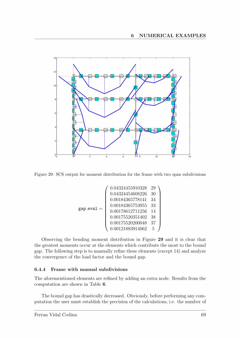
6 NUMERICAL EXAMPLES
−2 0 2 4 6 8 10 12 140
2
4
6
8
10
12
14
1
2
3
4
5
6
7
8
9
10
11
12
13
14
15
16
17
18
19
20
21
22
23
24
25
26
27
28
29
30
31
32
33
34
35
36
37 38
39 40
41 42
43 44
45 46
47 48
1
2
3
4
5
6
7
8
9
10
11
12
13
14
15
16
17
18
19
20
21
22
23
24
25
26
27
28 29 30 31
32 33 34 35
36 37 38 39
40 41 42 43
44 45 46 47
48 49 50 51
Figure 29: SCS output for moment distribution for the frame with two span subdivisions
gap eval =
0.04324455910328 290.04324454608226 300.00184365778141 340.00184365753955 330.00178612711256 140.00175520351402 380.00175520200048 370.00121883914062 5
Observing the bending moment distribution in Figure 29 and it is clear that
the greatest moments occur at the elements which contribute the most to the boundgap. The following step is to manually refine these elements (except 14) and analyzethe convergence of the load factor and the bound gap.
6.4.4 Frame with manual subdivisions
The aforementioned elements are refined by adding an extra node. Results from thecomputation are shown in Table 6.
The bound gap has drastically decreased. Obviously, before performing any com-putation the user must establish the precision of the calculations, i.e. the number of
Ferran Vidal Codina 69
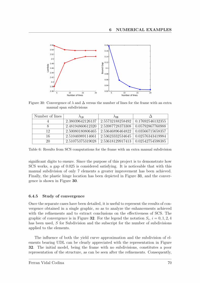
6 NUMERICAL EXAMPLES
5 10 15 202.36
2.38
2.4
2.42
2.44
2.46
2.48
2.5
2.52
2.54
2.56
Number of lines
Lam
bda
5 10 15 200.02
0.04
0.06
0.08
0.1
0.12
0.14
0.16
0.18
Number of lines
Bou
nd G
apFigure 30: Convergence of λ and ∆ versus the number of lines for the frame with an extra
manual span subdivisions
Number of lines λLB λUB ∆4 2.38039642126137 2.55732188258492 0.176925461323558 2.48194860612320 2.53987728373308 0.0579286776098812 2.50080180806465 2.53646896464822 0.0356671565835716 2.51046989114661 2.53623332534645 0.0257634341998420 2.51075375319028 2.53618129917413 0.02542754598385
Table 6: Results from SCS computations for the frame with an extra manual subdivision
significant digits to ensure. Since the purpose of this project is to demonstrate howSCS works, a gap of 0.025 is considered satisfying. It is noticeable that with thismanual subdivision of only 7 elements a greater improvement has been achieved.Finally, the plastic hinge location has been depicted in Figure 31, and the conver-gence is shown in Figure 30.
6.4.5 Study of convergence
Once the separate cases have been detailed, it is useful to represent the results of con-vergence obtained in a single graphic, so as to analyze the enhancements achievedwith the refinements and to extract conclusions on the effectiveness of SCS. Thegraphic of convergence is in Figure 32. For the legend the notation Si, i = 0, 1, 2, 4has been used, S for Subdivision and the subscript for the number of subdivisionsapplied to the elements.
The influence of both the yield curve approximation and the subdivision of el-ements bearing UDL can be clearly appreciated with the representation in Figure32. The initial model, being the frame with no subdivisions, constitutes a poorrepresentation of the structure, as can be seen after the refinements. Consequently,
Ferran Vidal Codina 70
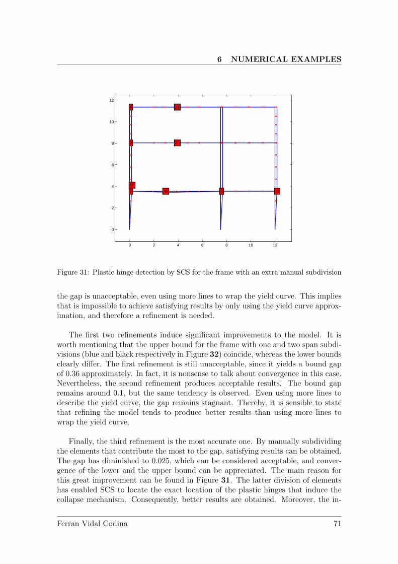
6 NUMERICAL EXAMPLES
0 2 4 6 8 10 12
0
2
4
6
8
10
12
4
662
5555
3
6 104949
2020
2121
Figure 31: Plastic hinge detection by SCS for the frame with an extra manual subdivision
the gap is unacceptable, even using more lines to wrap the yield curve. This impliesthat is impossible to achieve satisfying results by only using the yield curve approx-imation, and therefore a refinement is needed.
The first two refinements induce significant improvements to the model. It isworth mentioning that the upper bound for the frame with one and two span subdi-visions (blue and black respectively in Figure 32) coincide, whereas the lower boundsclearly differ. The first refinement is still unacceptable, since it yields a bound gapof 0.36 approximately. In fact, it is nonsense to talk about convergence in this case.Nevertheless, the second refinement produces acceptable results. The bound gapremains around 0.1, but the same tendency is observed. Even using more lines todescribe the yield curve, the gap remains stagnant. Thereby, it is sensible to statethat refining the model tends to produce better results than using more lines towrap the yield curve.
Finally, the third refinement is the most accurate one. By manually subdividingthe elements that contribute the most to the gap, satisfying results can be obtained.The gap has diminished to 0.025, which can be considered acceptable, and conver-gence of the lower and the upper bound can be appreciated. The main reason forthis great improvement can be found in Figure 31. The latter division of elementshas enabled SCS to locate the exact location of the plastic hinges that induce thecollapse mechanism. Consequently, better results are obtained. Moreover, the in-
Ferran Vidal Codina 71
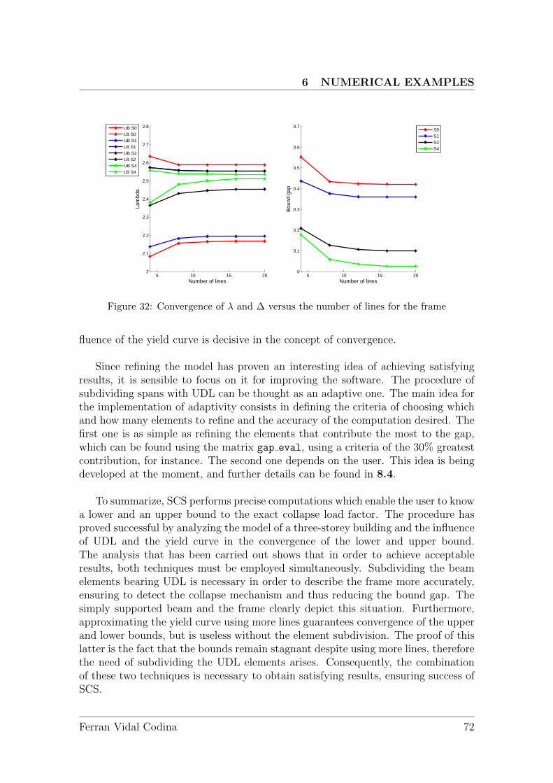
6 NUMERICAL EXAMPLES
5 10 15 202
2.1
2.2
2.3
2.4
2.5
2.6
2.7
2.8
Number of lines
Lam
bda
UB S0LB S0UB S1LB S1UB S2LB S2UB S4LB S4
5 10 15 200
0.1
0.2
0.3
0.4
0.5
0.6
0.7
Number of linesB
ound
gap
S0S1S2S4
Figure 32: Convergence of λ and ∆ versus the number of lines for the frame
fluence of the yield curve is decisive in the concept of convergence.
Since refining the model has proven an interesting idea of achieving satisfyingresults, it is sensible to focus on it for improving the software. The procedure ofsubdividing spans with UDL can be thought as an adaptive one. The main idea forthe implementation of adaptivity consists in defining the criteria of choosing whichand how many elements to refine and the accuracy of the computation desired. Thefirst one is as simple as refining the elements that contribute the most to the gap,which can be found using the matrix gap eval, using a criteria of the 30% greatestcontribution, for instance. The second one depends on the user. This idea is beingdeveloped at the moment, and further details can be found in 8.4.
To summarize, SCS performs precise computations which enable the user to knowa lower and an upper bound to the exact collapse load factor. The procedure hasproved successful by analyzing the model of a three-storey building and the influenceof UDL and the yield curve in the convergence of the lower and upper bound.The analysis that has been carried out shows that in order to achieve acceptableresults, both techniques must be employed simultaneously. Subdividing the beamelements bearing UDL is necessary in order to describe the frame more accurately,ensuring to detect the collapse mechanism and thus reducing the bound gap. Thesimply supported beam and the frame clearly depict this situation. Furthermore,approximating the yield curve using more lines guarantees convergence of the upperand lower bounds, but is useless without the element subdivision. The proof of thislatter is the fact that the bounds remain stagnant despite using more lines, thereforethe need of subdividing the UDL elements arises. Consequently, the combinationof these two techniques is necessary to obtain satisfying results, ensuring success ofSCS.
Ferran Vidal Codina 72
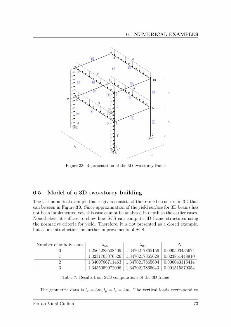
6 NUMERICAL EXAMPLES
lz
lx
ly
p
pq
q
xy
z 1
2
3
4 5
6
7
8
1
5
2
63
7
84
9
10
11
12 1613
14
15
9
10
11
12 q
q
lz
Figure 33: Representation of the 3D two-storey frame
6.5 Model of a 3D two-storey building
The last numerical example that is given consists of the framed structure in 3D thatcan be seen in Figure 33. Since approximation of the yield surface for 3D beams hasnot been implemented yet, this case cannot be analysed in depth as the earlier cases.Nonetheless, it suffices to show how SCS can compute 3D frame structures usingthe normative criteria for yield. Therefore, it is not presented as a closed example,but as an introduction for further improvements of SCS.
Number of subdivisions λLB λUB ∆0 1.2564283508409 1.3470217865156 0.0905934356741 1.3231703376526 1.3470217865629 0.0238514489102 1.3409786711463 1.3470217865604 0.0060431154143 1.3455059072096 1.3470217865643 0.001515879354
Table 7: Results from SCS computations of the 3D frame
The geometric data is lx = 3m, ly = lz = 4m. The vertical loads correspond to
Ferran Vidal Codina 73
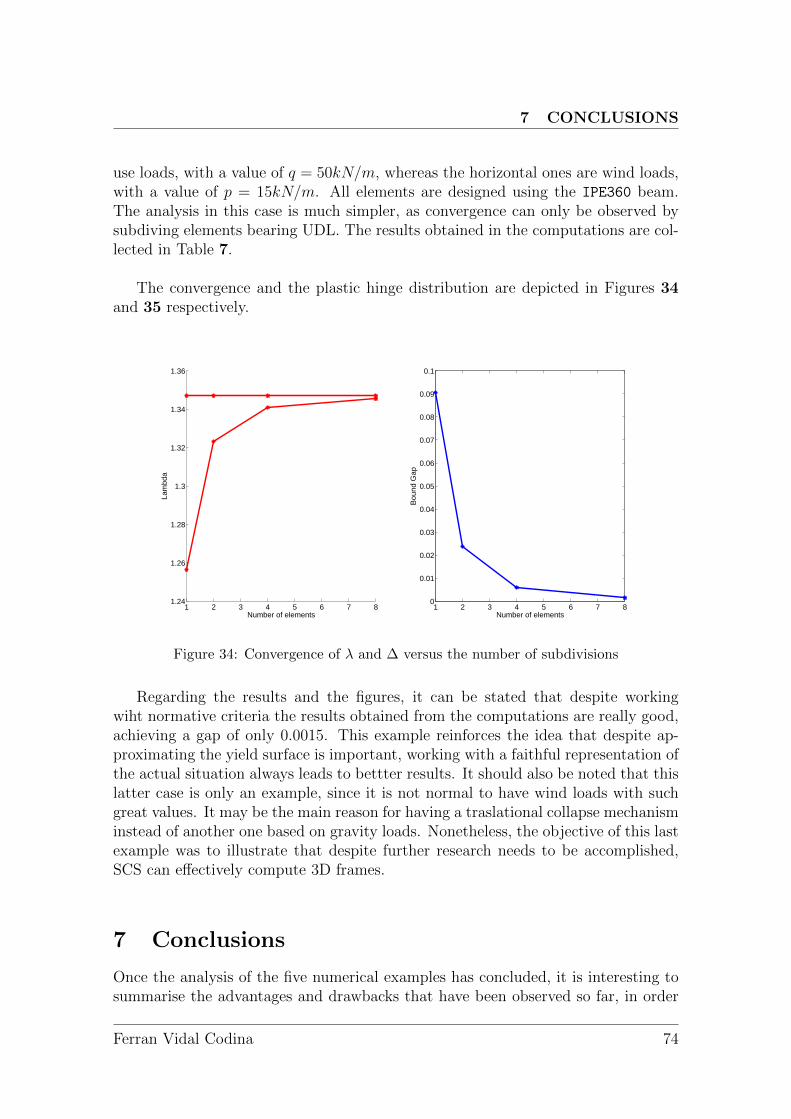
7 CONCLUSIONS
use loads, with a value of q = 50kN/m, whereas the horizontal ones are wind loads,with a value of p = 15kN/m. All elements are designed using the IPE360 beam.The analysis in this case is much simpler, as convergence can only be observed bysubdiving elements bearing UDL. The results obtained in the computations are col-lected in Table 7.
The convergence and the plastic hinge distribution are depicted in Figures 34and 35 respectively.
1 2 3 4 5 6 7 81.24
1.26
1.28
1.3
1.32
1.34
1.36
Number of elements
Lam
bda
1 2 3 4 5 6 7 80
0.01
0.02
0.03
0.04
0.05
0.06
0.07
0.08
0.09
0.1
Number of elements
Bou
nd G
ap
Figure 34: Convergence of λ and ∆ versus the number of subdivisions
Regarding the results and the figures, it can be stated that despite workingwiht normative criteria the results obtained from the computations are really good,achieving a gap of only 0.0015. This example reinforces the idea that despite ap-proximating the yield surface is important, working with a faithful representation ofthe actual situation always leads to bettter results. It should also be noted that thislatter case is only an example, since it is not normal to have wind loads with suchgreat values. It may be the main reason for having a traslational collapse mechanisminstead of another one based on gravity loads. Nonetheless, the objective of this lastexample was to illustrate that despite further research needs to be accomplished,SCS can effectively compute 3D frames.
7 Conclusions
Once the analysis of the five numerical examples has concluded, it is interesting tosummarise the advantages and drawbacks that have been observed so far, in order
Ferran Vidal Codina 74
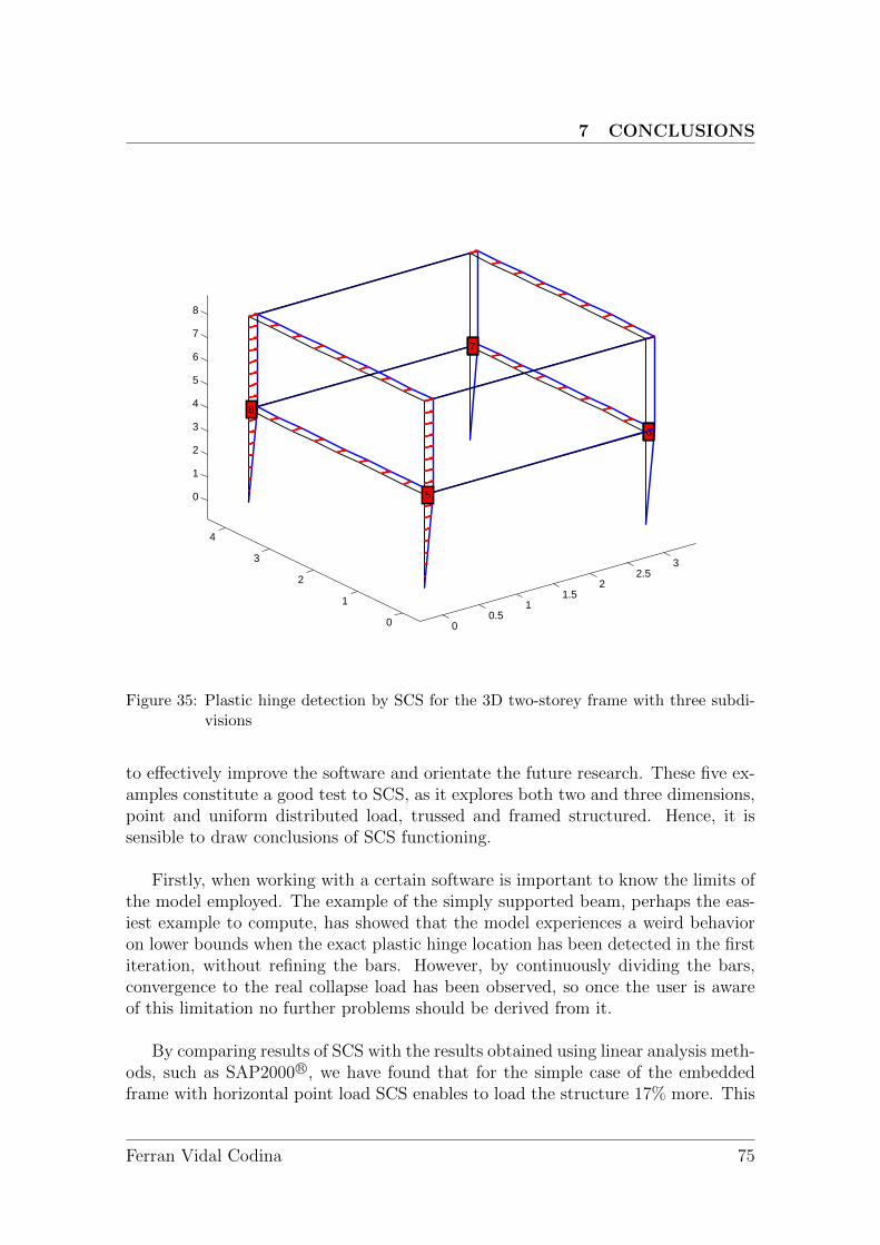
7 CONCLUSIONS
00.5
11.5
22.5
3
0
1
2
3
4
0
1
2
3
4
5
6
7
8
6666
7777
55
88
Figure 35: Plastic hinge detection by SCS for the 3D two-storey frame with three subdi-visions
to effectively improve the software and orientate the future research. These five ex-amples constitute a good test to SCS, as it explores both two and three dimensions,point and uniform distributed load, trussed and framed structured. Hence, it issensible to draw conclusions of SCS functioning.
Firstly, when working with a certain software is important to know the limits ofthe model employed. The example of the simply supported beam, perhaps the eas-iest example to compute, has showed that the model experiences a weird behavioron lower bounds when the exact plastic hinge location has been detected in the firstiteration, without refining the bars. However, by continuously dividing the bars,convergence to the real collapse load has been observed, so once the user is awareof this limitation no further problems should be derived from it.
By comparing results of SCS with the results obtained using linear analysis meth-ods, such as SAP2000 R©, we have found that for the simple case of the embeddedframe with horizontal point load SCS enables to load the structure 17% more. This
Ferran Vidal Codina 75
7 CONCLUSIONS
fact illustrates the convenience of employing SCS for collapse computations, sinceit finds the load factor necessary for the structure to collapse and the real collapsemechanism. Linear elastic methods, however, only find the first plastic hinge toform. Moreover, it does not only give a greater collapse load, but also bounds itupper and lower as precisely as the user desires. This case and the steel tower justifythe use of SCS in structure limit analysis.
Finally, once clarified the limits of the model and the justification of employ-ment, a 2D and a 3D frame have been computed in order to study the influenceof several parameters in the convergence of the load factor. The theoretical basisstates that bounding of the actual load factor comes from approximating the yieldcurve/surface of each beam element inwards or outwards and from considerating asecant and a tangent moment distribution to the actual one in UDL elements. In thelast two examples the influence of each factor has been widely studied. According tothe results obtained, it is clear that refining the UDL elements leads to much betterresults than the ones obtained by refining the yield surface. By subdividing the UDLelements, the actual moment distribution is progressively approximated, with thegap diminishing with the square of the beam length. This fact explains the resultsobtained. Nonetheless, it is advisable to combine both bounding techniques in orderto obtain the best results possible. This influence is best observed in Figure 32. Byimproving the yield criteria results slightly get better, although refining the UDL ele-ments -i.e. having a more representative model- is decisive in achieving convergence.
To conclude, SCS is a powerful tool that computes all kind of trussed and framedstructures using plastic analysis, offering a bounding as precise as desired of theload that induces collapse in the structure. It enables the user to perform strongercomputations than the ones with elastic methods, as well as being able to combinetwo different methods of bounding the load factor for more efficient computations.
Ferran Vidal Codina 76
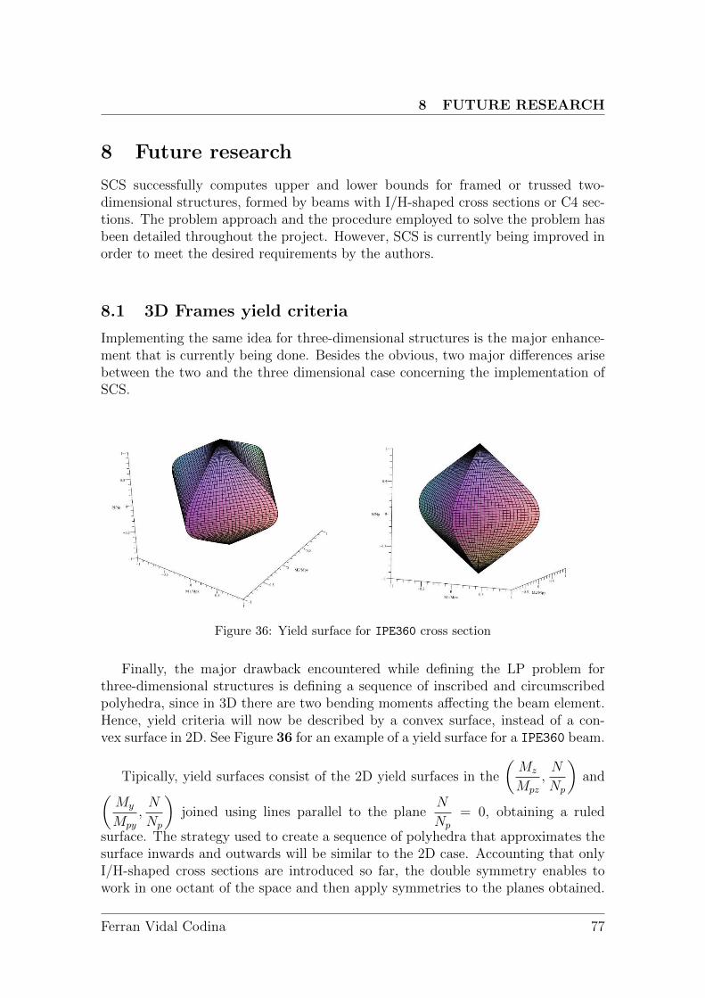
8 FUTURE RESEARCH
8 Future research
SCS successfully computes upper and lower bounds for framed or trussed two-dimensional structures, formed by beams with I/H-shaped cross sections or C4 sec-tions. The problem approach and the procedure employed to solve the problem hasbeen detailed throughout the project. However, SCS is currently being improved inorder to meet the desired requirements by the authors.
8.1 3D Frames yield criteria
Implementing the same idea for three-dimensional structures is the major enhance-ment that is currently being done. Besides the obvious, two major differences arisebetween the two and the three dimensional case concerning the implementation ofSCS.
Figure 36: Yield surface for IPE360 cross section
Finally, the major drawback encountered while defining the LP problem forthree-dimensional structures is defining a sequence of inscribed and circumscribedpolyhedra, since in 3D there are two bending moments affecting the beam element.Hence, yield criteria will now be described by a convex surface, instead of a con-vex surface in 2D. See Figure 36 for an example of a yield surface for a IPE360 beam.
Tipically, yield surfaces consist of the 2D yield surfaces in the
(Mz
Mpz
,N
Np
)and(
My
Mpy
,N
Np
)joined using lines parallel to the plane
N
Np
= 0, obtaining a ruled
surface. The strategy used to create a sequence of polyhedra that approximates thesurface inwards and outwards will be similar to the 2D case. Accounting that onlyI/H-shaped cross sections are introduced so far, the double symmetry enables towork in one octant of the space and then apply symmetries to the planes obtained.
Ferran Vidal Codina 77
8 FUTURE RESEARCH
The technique for creating the polyhedra approximating the yield surface is currentlybeing developed.
8.2 Cross Section Library
Besides implementing the 3D case, there is a concern for widening the range ofcross sections available to use in the computations. I/H-shaped cross sections andC4 sections are perhaps the most commonly used, but regardless this condition apowerful program must offer the maximum number of possibilities to the user. InSection (4.2.2) sections with T, L and U are mentioned. The first one is currentlybeing studied, and the expression of the yield surface has been analytically found.The problem encountered is that it differs from the I/H-shaped sections that itcannot be written explicitly, i.e. the moment as a function of the axial stress orviceversa. The fact that the yield surface is an implicit function of M
Mp, N
Npimpedes
to use the Newton-Raphson routine employed for the explicit case. One of the maingoals is to adapt the technique in order to make it able to operate with implicitfunctions. The case of L and U is quite different, since the analytical formulae havenot been found yet, although it constitutes another point of major interest. Once theyield surface is written, they will likely be easily studied with the Newton-Raphsontechnique for implicit functions.
8.3 LP solver
The routine linsolve in Matlab R© is the one currently used to resolve both the upperand the lower bound problems. For the cases studied it has provided satisfyingresults within reasonable time. In fact, the case that took longer to compute isthe one described in Section 6.4.4 with 20 lines approximating the yield surfaceper node, and the computation time was around 20 s. Nonetheless, the final goalof SCS is to compute complex 3D framed structures with hundreds or thousandsof elements. At this extent, linsolve would probably not only be slow, but alsoinsufficient to assure convergence. The authors’ idea is to introduce the convexoptimization package SDPT3 to achieve a better performance of the LP solver.The main difficulty nowadays is that the LP problems (14) and (15) are describedin the general LP form, see (4), and SDPT3 package requires the problem to beexpressed with nonnegative variables and equality constraints. Even though it doesnot suppose a great effort to transform the existing problems into ones that fit thischaracteristics by using slack variables, it is a procedure that has not been developedyet, and it will gain interest as the 3D case reaches to completion.
8.4 Adaptivity
Throughout the project it has been proven repeatedly the importance of refining theelements bearing UDL in a framed structure, in order to reduce the bound gap inthe computations. Nonetheless, the procedure of refining is nowadays hand-driven,
Ferran Vidal Codina 78
8 FUTURE RESEARCH
and hence it may result tedious when precise computations have to be carried out.The authors’ idea is to transform SCS into an iterative method where the user wouldset manually the precision desired in the computation, and the program would useadaptivity to improve the computations after each iteration. The basic idea ofadaptivity applied to SCS consists of locating after each iteration the elements thatcontribute the most to the gap, i.e. the top rows of the matrix gap eval. Thecriteria employed for selecting how many elements should be refined would also bea user’s choice. Thereby, after each iteration SCS would refine the selected bars, ameasure that can be complemented with improving the approximation of the yieldcurve/surface. Using adaptivity, SCS would not only be more efficient, but alsoeasier and faster to be used, since the work of entering the structure informationwould only be done once.
Ferran Vidal Codina 79
REFERENCES
References
[1] S. Boyd and L. Vandenberghe, Convex optimization. Cambridge UniversityPress, Cambridge, 1994.
[2] H. Maier and Leibnitz, Versuche mit eingespannten und einfachen Balken vonI-Form aus St. 37, vol. 7. Bautechnik, 1929.
[3] H. Greenberg and W. Prager, “On limit design of beams and frames,” Proc.ASCE, vol. 77, no. 59, 1951.
[4] B. Neal and P. Symonds, “The calculations of collapse loads for framed struc-tures,” J Inst Civil Eng, 1951.
[5] B. Neal and P. Symonds, “The rapid calculation of plastic collapse loads fora framed structure,” Proceedings of the institution of civil engineers London,vol. 1, no. 3, pp. 58–100, 1952.
[6] B. Neal and P. Symonds, “Recent progress in the plastic methods of structuralanalysis,” Journal of the Franklin Institute, vol. 252, pp. 383–407, November1951.
[7] E. Chwalla, “Three contributions to the problem of the load carrying capacityof statically indeterminate steel frames,” Publ. of Intern. Assn. Bridge andStructural Engrg. Zurich, Switzerland, vol. 2, pp. 96–125, 1933-34.
[8] M. Baker, J.F. Horne and J. Roderick, “The behaviour of continuous stan-chions,” Royal Society, vol. 198, p. 493, 1949.
[9] A. Charnes and H. Greenberg Bull. Amer. Math. Soc., vol. 57, 1951.
[10] C. Charnes, A. Lemke and O. Zienkiewicz, “Virtual work, linear programmingand plastic limit analysis,” Royal Society, vol. 251, pp. 110–116, May 1959.
[11] J. Heyman, “On the minimum weight design of a simple portal frame,” Int JMech Sci, 1960.
[12] M. Horne, “Determination of the shape of fixed ended beams for maximumeconomy according to the plastic theory,” fourth congress, final report, Inter-national association of bridge and structural engineering, 1953.
[13] J. Baker and J. Heyman, Plastic design of frames, fundamentals, vol. 1. Cam-bridge University Press, 1969.
[14] V. Watwood, “Mechanism generation for limit analysis of frames,” Journal ofthe Structural Division, vol. 105, pp. 1–15, January 1979.
Ferran Vidal Codina 80
REFERENCES
[15] E. Anderheggen and H. Knopfel, “Finite element limit analysis using linearprogramming,” International Journal of Solids and Structures, vol. 8, pp. 1413–1431, January 1972.
[16] J. Munro, “Optimal plastic design of frames,” 71-136, Proceedings of NATO,Waterloo: Advanced Study in Engineering Plasticity by Mathematical Pro-gramming, 1977.
[17] R. Livesley, Linear programming in structural analysis and design. Wiley, 1977.
[18] S. Maier, G. Giacomini and F. Paterlini, “Combined elastoplastic and limitanalysis via restricted basis linear programming,” Computer methods in appliedmathematics and engineering, vol. 19, pp. 21–48, 1979.
[19] A. Jennings and T. Tam, “Automatic plastic design of frames,” EngineeringStructures, vol. 8, 1986.
[20] G. Thierauf, “A method for optimal limit design of structures withalternat iveloads.,” Computer methods in applied mathematics and engineering, vol. 16,pp. 49–134, 1987.
[21] L. Damkilde and O. Hoyer, “An efficient implementation of limit state calcula-tions based on lower-bound solutions,” Computers & Structures, vol. 49, no. 6,pp. 953–962, 1993.
[22] F. Tin-Loi, “Plastic limit analysis of plane frames and grids using gams,” Com-puters & Structures, vol. 54, no. 1, pp. 15–25, 1995.
[23] A. Kaveh and M. Jahanshahi, “Plastic limit analysis of frames using ant colonysystems,” Computers & Structures, vol. 86, pp. 1152–1163, 2008.
[24] L. Corradi, L. Luzzi and P. Vena, “Finite element limit analysis of anisotropicstructures,” Computer methods in applied mathematics and engineering,vol. 195, pp. 5422–5436, 2006.
[25] T. Tjhin and A. Kuchma, “Integrated analysis and design tool for the strut-and-tie method,” Engineering Structures, vol. 29, pp. 3042–3052, March 2007.
[26] H. Van Long and N. Dang Hung, “Limit and shakedown analysis of 3d steelframes,” Engineering Structures, vol. 30, pp. 1895–1904, January 2008.
[27] J. Ciria, H. Peraire and J. Bonet, “Mesh adaptive computation of upper andlower bounds in limit analysis,” International Journal for Numerical Methodsin Engineering, vol. 75, pp. 899–904, January 2008.
[28] N. Borges, L.A. Zouain and A. Huespe, “A nonlinear optimization procedurefor limit analysis,” European Journal of Mechanics, vol. 15, no. 3, p. 487512,1996.
Ferran Vidal Codina 81

REFERENCES
[29] A. Lyamin and S. Sloan, “Lower bound limit analysis using non-linear program-ming,” International Journal for Numerical Methods in Engineering, vol. 55,pp. 573–611, 2002.
[30] K. Krabbenhoft and L. Damkilde, “A general nolinear optimization algorithmfor lower bound limit analysis,” International Journal for Numerical Methodsin Engineering, vol. 56, pp. 84–165, 2003.
Ferran Vidal Codina 82


![Flexible Load Balancing with Multi-dimensional State-space Collapse: Throughput … · 2020. 4. 28. · Given a throughput optimal load balancing policy, if there exists an 2(0;1]](https://static.fdocument.org/doc/165x107/60f8d6ad82289657c10a2577/flexible-load-balancing-with-multi-dimensional-state-space-collapse-throughput.jpg)