Ongoing calibration and extension of SST 4 and 11 μm waveband algorithms for AQUA and TERRA MODIS using the in situ buoy,

radiometer matchup database

Robert EvansGuilllermo Podesta’

RSMASMay 17-20, 2011

with special thanks to R. Reynolds forthe provision of AVHRR OI reference fields

andChelle Gentemann

for provision of AMSR fields

Proposal Activities - Maintenance Component

• Update MODIS SST algorithm coefficients and uncertainty estimates (Hypercube) based on new MCST calibration “collection 6.”

• Monitor and validate SST retrievals for MODIS AQUA and TERRA with respect to in situ observations to enable calculation of a seamless climate-quality data record.

• Maintain and update the MODIS SST Matchup Database.• New Hypercube and algorithm coefficient tables based on

the MCST Collection 6 MODIS calibration have been computed and are being tested. Delivery to OBPG will follow.

Development of Version 6, Collection 6 SST algorithm

Correction to SST4 bias resulting from TERRA configuration changes

Upper and middle panels: MODIS-Terra calibration changes for channels 20 and 22.

Lower panel: Median of SST4 residuals estimated using 4µ channels. In all panels the x-axis indicates time. It is clear that calibration issues during 2000 and 2001 had considerable impact on SST retrievals based on 4µm bands.

MODIS TERRA Mirror side and Scan Angle corrections to SST

(analogous corrections computed for AQUA)

Terra mirror side

offset order 0.1K

Terra cross-scan correction order

0.15K

Colors indicatemagnitude ofResiduals, K

Description of LATBAND formulation and Matchup criteria

LATBANDLatitude

increments

•MODIS Version 6 (+Collection 6 calibration) based on LATBAND formulation – 6 zonal bands 20 degrees wide centered on the Equator•2.5 degree wide transition band, linearly interpolated•Coefficients estimated monthly, e.g. all January sat-in situ observations grouped, for each month of all years for a given sensor•Matchup criteria – within 2km and ±30 minutes for buoy-satellite observation•Skin temperature product•SST retrievals validated againstradiometer matchups (M-AERI)

Comparison of Version 5 & 6, AQUA(after correction for mirror side, scan angle)

Time series of mean SST residuals for MODIS-Aqua. SSTs were calculated using algorithm coefficients estimated separately for six fixed latitudinal bands and for each month of the year. This approach is referred to as the “LATBAND” approach.

Lower panel: mean SST residuals for MODIS-Aqua calculated using the current (Version 5) formulation of the MODIS SST algorithm. It is clear that the latitude-specific coefficients contribute to lower and more stable values of retrieval bias.

Version 6

Version 5

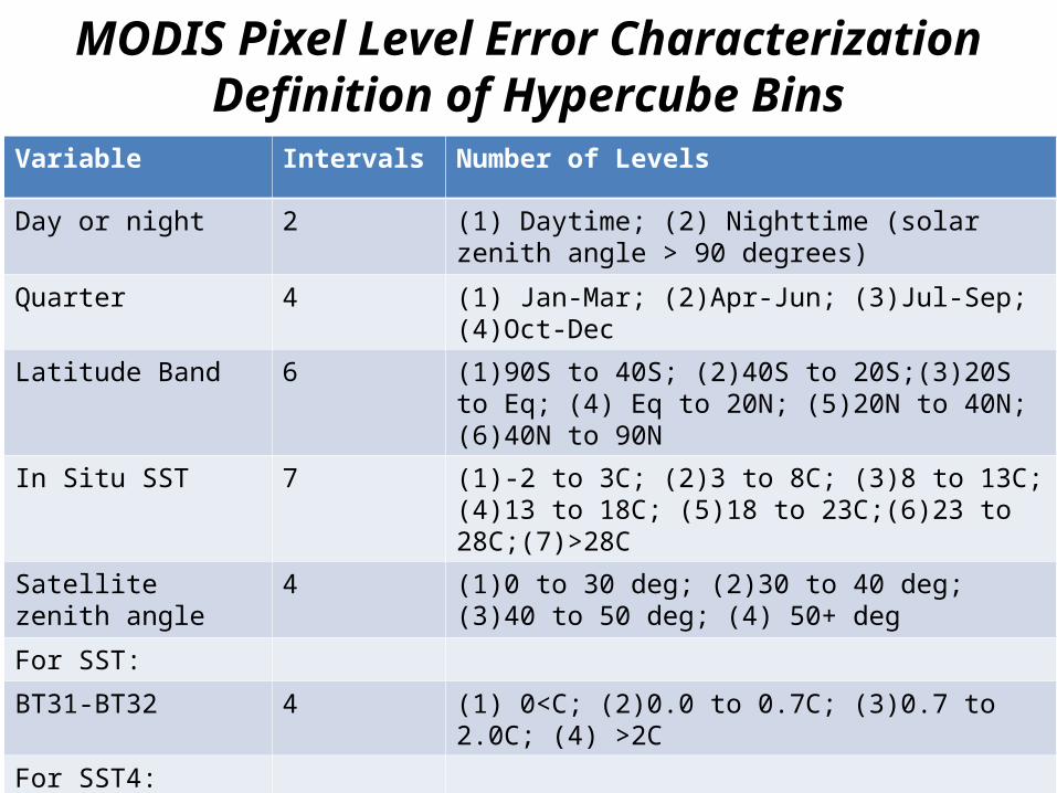
MODIS Pixel Level Error CharacterizationDefinition of Hypercube Bins

Variable Intervals Number of Levels

Day or night 2 (1) Daytime; (2) Nighttime (solar zenith angle > 90 degrees)

Quarter 4 (1) Jan-Mar; (2)Apr-Jun; (3)Jul-Sep; (4)Oct-Dec

Latitude Band 6 (1)90S to 40S; (2)40S to 20S;(3)20S to Eq; (4) Eq to 20N; (5)20N to 40N; (6)40N to 90N

In Situ SST 7 (1)-2 to 3C; (2)3 to 8C; (3)8 to 13C; (4)13 to 18C; (5)18 to 23C;(6)23 to 28C;(7)>28C

Satellite zenith angle 4 (1)0 to 30 deg; (2)30 to 40 deg; (3)40 to 50 deg; (4) 50+ deg

For SST:

BT31-BT32 4 (1) 0<C; (2)0.0 to 0.7C; (3)0.7 to 2.0C; (4) >2C

For SST4:

BT22-BT21 4 (1)0.0 to 2.0C; (2)2.0 to 3.0C; (3)3.0 to 4.0C; (4) >4.0C

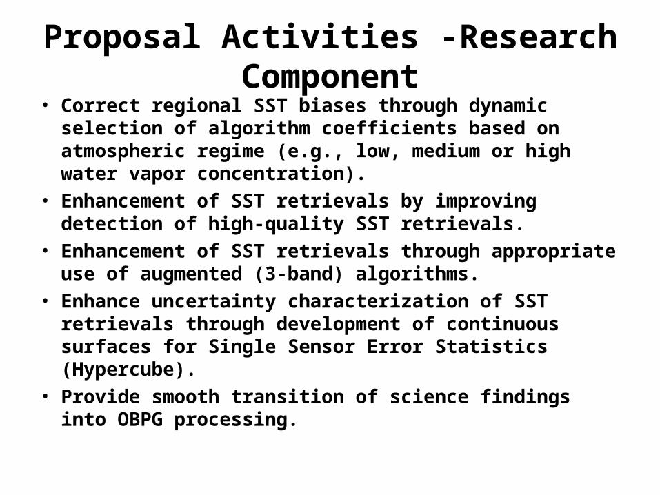
Proposal Activities -Research Component• Correct regional SST biases through dynamic selection of

algorithm coefficients based on atmospheric regime (e.g., low, medium or high water vapor concentration).

• Enhancement of SST retrievals by improving detection of high-quality SST retrievals.

• Enhancement of SST retrievals through appropriate use of augmented (3-band) algorithms.

• Enhance uncertainty characterization of SST retrievals through development of continuous surfaces for Single Sensor Error Statistics (Hypercube).

• Provide smooth transition of science findings into OBPG processing.

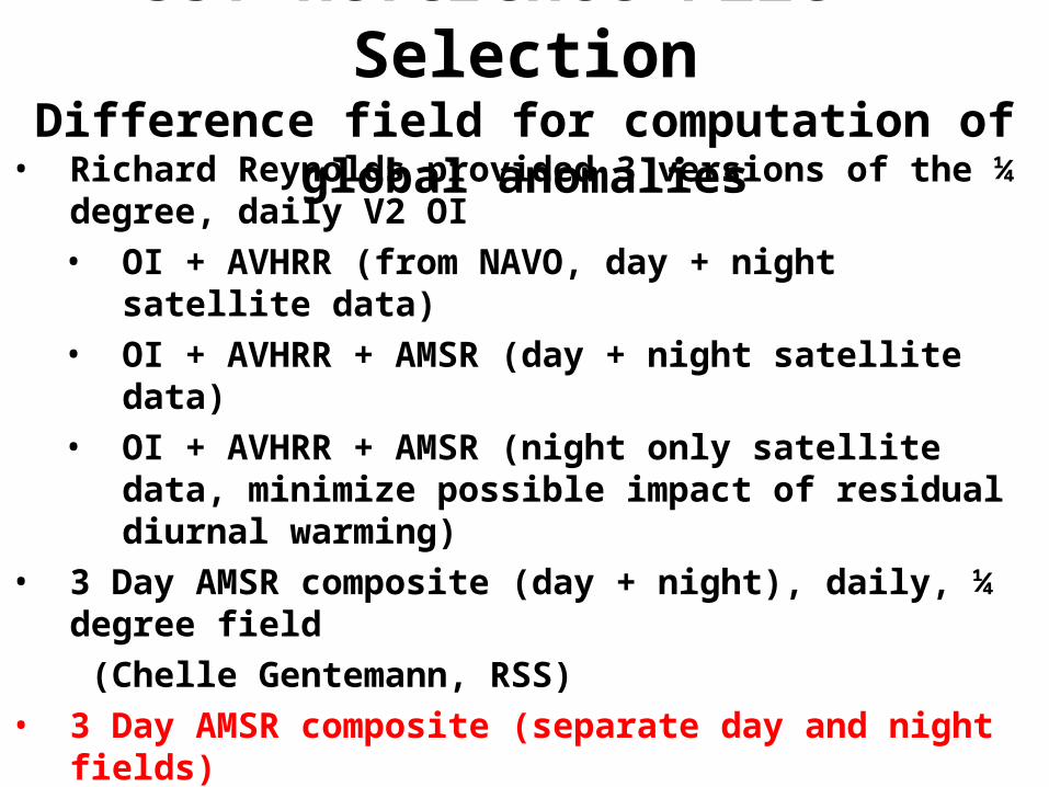
SST Reference File – SelectionDifference field for computation of global anomalies• Richard Reynolds provided 3 versions of the ¼ degree, daily V2 OI

• OI + AVHRR (from NAVO, day + night satellite data)• OI + AVHRR + AMSR (day + night satellite data)• OI + AVHRR + AMSR (night only satellite data, minimize

possible impact of residual diurnal warming)• 3 Day AMSR composite (day + night), daily, ¼ degree field

(Chelle Gentemann, RSS)• 3 Day AMSR composite (separate day and night fields)• AATSR (night only), based on 0.1 degree night only, 3 channel,

dual view product (processing version: May, 2010)• R . Reynolds processed AATSR daily fields into monthly, ¼

degree maps to fill gaps due to combination of narrow swath and cloudy observing conditions

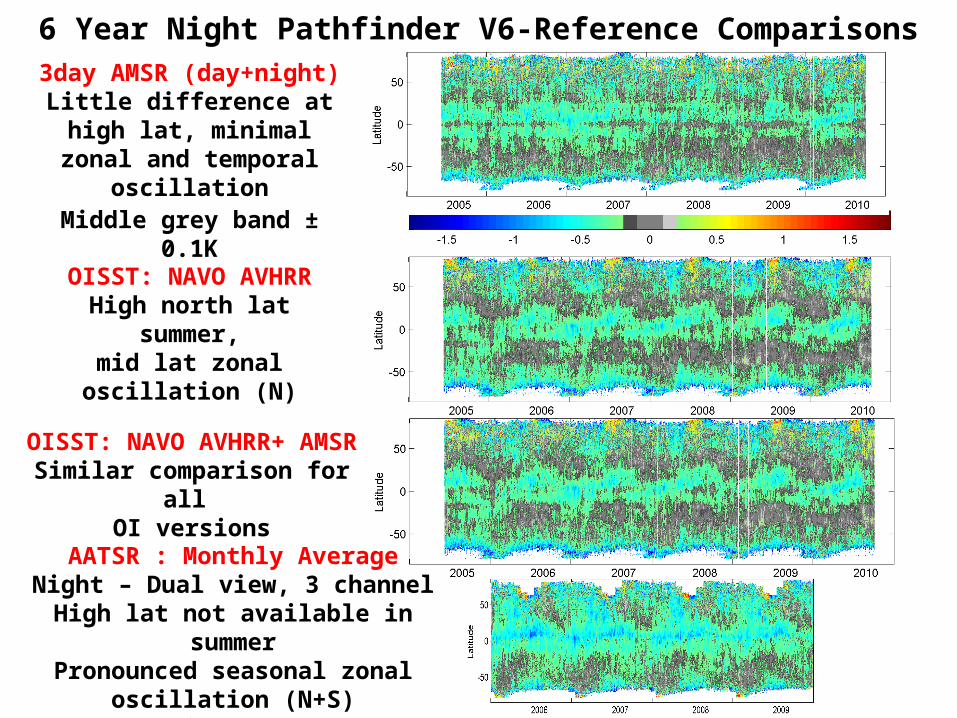
6 Year Night Pathfinder V6-Reference Comparisons3day AMSR (day+night)

Little difference at high lat, minimal zonal and temporal

oscillation

OISST: NAVO AVHRRHigh north lat summer,

mid lat zonal oscillation (N)

OISST: NAVO AVHRR+ AMSRSimilar comparison for all

OI versions

Middle grey band ± 0.1K

AATSR : Monthly AverageNight – Dual view, 3 channel

High lat not available in summerPronounced seasonal zonal oscillation (N+S)

N equatorial aerosol more pronounced

Impact of diurnal warming on comparison to reference fields

Anomaly fields show significant difference whena single reference field is used for both day and nightsatellite fields

Anomaly fields are very similar when reference field is temporally matched to satellite observation time

Path V6 – 3day AMSR composite (single field for 24 hours)

Path V6- Reynolds OI (single field for 24 hours)

Path V6 – AMSR 3 day composite, separate day and night

Day

Night

Day

N18 PF6-AMSR (night only) monthly, best quality, 2006Residual patterns evolve month to month

MarJan

May Jul

Sep Nov

Version 7 SST algorithm• Version 7 will retain the 6 regions use by the

Version 6 LATBAND algorithm but will use the 11-12μm brightness temperature difference (water vapor proxy) to select region boundaries, 3 each in the northern and southern hemispheres to minimize seasonal, regional anomalies.

• Hypercube implementation for Version 6 uses discrete intervals for the selection variables. Version 7 will use smoothly varying parameterization for scan angle, brightness temperature difference and temperature

Comparison of 3 band vs 2 band SST4Difference fields between MODIS Aqua SST4 (2 July 2006) and corresponding Reynolds V2 SST analysis.

The upper panel is based on a two-band (3.95 and 4.05 μm bands) LATBAND SST4 algorithm.

The lower panel is based on a three-band SST4 algorithm incorporating data from the 3.75μm band. The color scale at right goes from -3 to +3 K.

Conclusions•Collection 6 based Version 6 SST LATBAND algorithm coefficients and uncertainty Hypercube being validated for AQUA and TERRA. Delivery to OBPG will follow.•Use of reference fields temporally matched to the satellites minimizes the magnitude of residual patterns,AMSR 3 day composite day and night fields are the preferred reference SST field.•A Version 7 SST algorithm will be investigated to determine if the residual seasonal, regional anomalies are minimized.•Implementation of a smoothed field Hypercube will be investigated to remove field discontinuities present in the current discrete implementation•The 3 band SST4 algorithm will be tested to validate its ability to more completely address identification and correction of dust aerosol influence.•SeaDAS now has LATBAND support for MODIS, VIIRS and AVHRR.

END

Use of homogeneity and channel difference to develop a probability tree to assign quality level –

PF6

Q=0Q=1Q=4 Q=3

Example of using a probability distribution approach to assign quality.Implementation of this approach will require exploration of multiple categories, e.g. small; large residuals

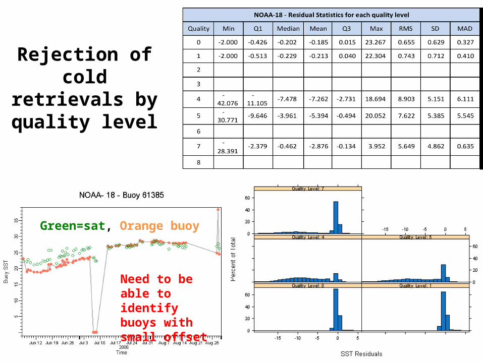
Rejection of cold retrievals by quality

level

Green=sat, Orange buoy

Need to be able to identify buoys with small offset

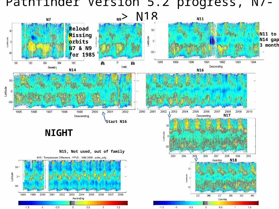
Pathfinder Version 5.2 progress, N7-> N18

N15, Not used, out of family

NIGHT

N16

N18

N7 N9 N11

N14

Reload MissingorbitsN7 & N9for 1985

N11 toN14 gap3 month

N17

Start N16

86 88

Comparison of 1 day Pathfinder vs ref fields

3day AMSR reference

OISST (NAVO AVHRR ) reference

Monthly AATSR referenceNight, Dual view, 3 channel

July 19, 2009 N18 night

Note differences, Med, high lat

Anomalies reasonably consistent across satellites although diurnal

variability is present

Monthly DT field, Pathfinder V6 – 3 day AMSR (separate Day and Night reference) for January 2006

N18-AMSR NNight

N18-AMSR DDay

N17-AMSR DMorning

N17-AMSR NEvening

Color step = 0.2K -.2 0 .2

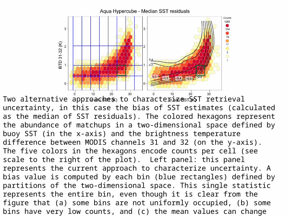
Two alternative approaches to characterize SST retrieval uncertainty, in this case the bias of SST estimates (calculated as the median of SST residuals). The colored hexagons represent the abundance of matchups in a two-dimensional space defined by buoy SST (in the x-axis) and the brightness temperature difference between MODIS channels 31 and 32 (on the y-axis). The five colors in the hexagons encode counts per cell (see scale to the right of the plot). Left panel: this panel represents the current approach to characterize uncertainty. A bias value is computed by each bin (blue rectangles) defined by partitions of the two-dimensional space. This single statistic represents the entire bin, even though it is clear from the figure that (a) some bins are not uniformly occupied, (b) some bins have very low counts, and (c) the mean values can change substantially between adjacent bins, leading to discontinuities in the retrieved uncertainty field. Right panel: In the proposed approach, a surface is fit to the median of residuals as a function of the two dimensions selected. Contour lines describe SST residual bias (values shown for 0.4K to -0.8K, every 0.2K). A rectangle overlaid on the contours (corresponding to one of the bins in the left panel) shows that the same bin may have a very broad range of bias values, and a single value fails to describe uncertainty adequately.