14.771 Development Economics: Microeconomic … marriage (e.g. random allocation of CCT transfers to...

MIT OpenCourseWarehttp://ocw.mit.edu

14.771 Development Economics: Microeconomic issues and Policy Models Fall 2008

For information about citing these materials or our Terms of Use, visit: http://ocw.mit.edu/terms.

http://ocw.mit.edu

http://ocw.mit.edu/terms

Testing Household Models

Esther Duflo

14.771

1 / 25

Outline

• Is the household unitary?

Is the household efficient? •

What next? •

2 / 25

Is the Household Unitary?

• Do things other than prices and overall resources (“distribution factors”) enter in the production function

• Most tests are test of “income pooling”: Does the identity of a transfer recipient matter?

• Other things can influence distribution inside the household: • Divorce Laws (Chiappori-Fortin-Lacroix) • Marriage markets (Angrist; Lafortune)

Labor market• • Assets brought to the wedding and that spouse retains control

of (Thomas-Frankenberg-Contreras)

3 / 25

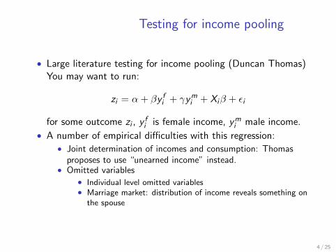
Testing for income pooling

• Large literature testing for income pooling (Duncan Thomas) You may want to run:

zi = α + βyfi + γymi + Xi β + �i

for some outcome zi , y fi is female income, ymi male income.

• A number of empirical difficulties with this regression: • Joint determination of incomes and consumption: Thomas

proposes to use “unearned income” instead.Omitted variables•

Individual level omitted variables • • Marriage market: distribution of income reveals something on

the spouse

4 / 25

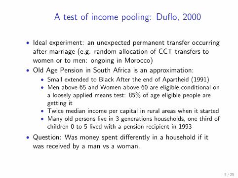
A test of income pooling: Duflo, 2000

• Ideal experiment: an unexpected permanent transfer occurring after marriage (e.g. random allocation of CCT transfers to women or to men: ongoing in Morocco)

• Old Age Pension in South Africa is an approximation: • Small extended to Black After the end of Apartheid (1991) • Men above 65 and Women above 60 are eligible conditional on

a loosely applied means test: 85% of age eligible people are getting it

• Twice median income per capital in rural areas when it started • Many old persons live in 3 generations households, one third of

children 0 to 5 lived with a pension recipient in 1993

• Question: Was money spent differently in a household if it was received by a man vs a woman.

5 / 25

Empirical strategy

• Outcome of interest: Children’s weight-for-age and height-for-age

• Children who live with pensioners live in different households than those who don’t (extended families are poorer, more rural, etc.).

• This may also differ for female vs male. • Two strategies:

• “Regression Discontinuity Design” using the age cutoffs for pension recipient for weight-for-height

• Difference-in-difference for the height-for-age

6 / 25

�

Weight for height

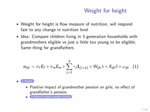
• Weight for height is flow measure of nutrition, will respond fast to any change in nutrition level

• Idea: Compare children living in 3 generation households with grandmothers eligible vs just a little too young to be eligible; Same thing for grandfathers

4

wijk = πf Ef + πmEm + γl 1(l=k) + Wijk λ + Xijk δ + ωijk (1) j=1

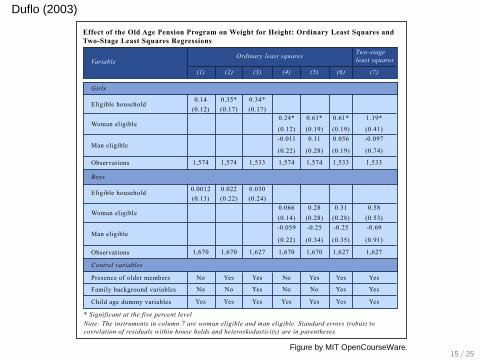
• Positive impact of grandmother pension on girls, no effect of grandfather’s pension

• Results

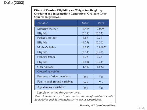
• Mother’s mother pension matters

7 / 25

� �

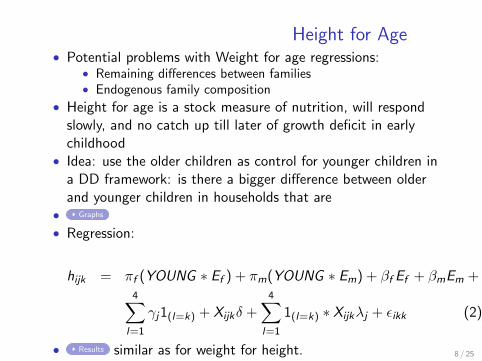
Height for Age • Potential problems with Weight for age regressions:

• Remaining differences between families • Endogenous family composition

• Height for age is a stock measure of nutrition, will respond slowly, and no catch up till later of growth deficit in early childhood

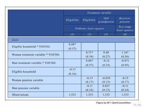
• Idea: use the older children as control for younger children in a DD framework: is there a bigger difference between older and younger children in households that are

• Regression:

hijk = πf (YOUNG ∗ Ef ) + πm(YOUNG ∗ Em) + βf Ef + βmEm + 4 4

γj 1(l=k) + Xijk δ + 1(l=k) ∗ Xijk λj + �ikk (2) l=1 l=1

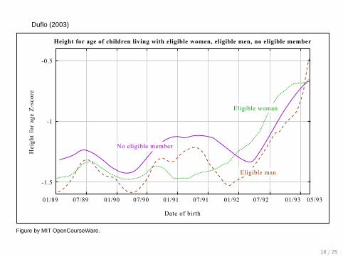
• Graphs

• Results similar as for weight for height. 8 / 25

Household Efficiency: Ratio tests

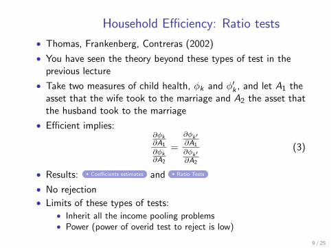
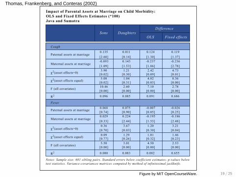
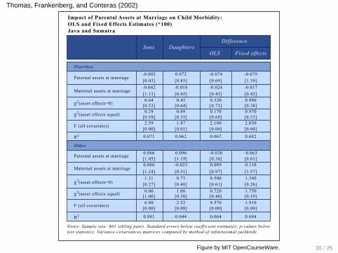
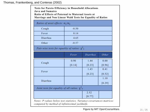
• Thomas, Frankenberg, Contreras (2002)

• You have seen the theory beyond these types of test in the previous lecture

Take two measures of child health, φk and φ� , and let A1 the• k asset that the wife took to the marriage and A2 the asset thatthe husband took to the marriage

• Efficient implies: ∂φk ∂φk� ∂A1 ∂A1= (3)∂φk ∂φk�∂A2 ∂A2

Ratio Tests

• No rejection • Limits of these types of tests:

• Inherit all the income pooling problems • Power (power of overid test to reject is low)

9 / 25

• Results: Coefficients estimates and

Household Efficiency: Production Efficiency

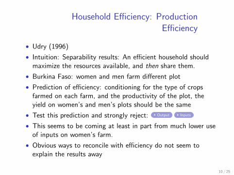
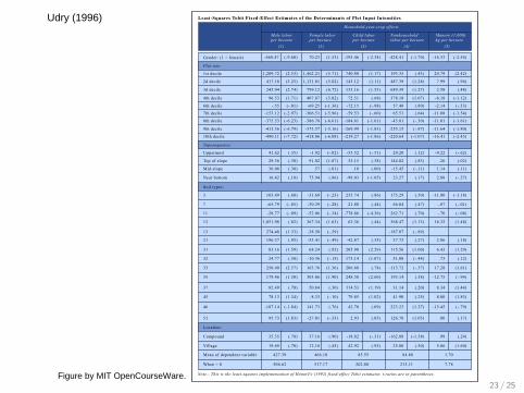
• Udry (1996)

• Intuition: Separability results: An efficient household should maximize the resources available, and then share them.

• Burkina Faso: women and men farm different plot

• Prediction of efficiency: conditioning for the type of crops farmed on each farm, and the productivity of the plot, the yield on women’s and men’s plots should be the same

• Test this prediction and strongly reject: Output Inputs

• This seems to be coming at least in part from much lower use of inputs on women’s farm.

• Obvious ways to reconcile with efficiency do not seem to explain the results away

10 / 25

• What is the likely source of violation of efficiency here? • Household looks at income brought by each household member

(rather than potential income). Household member invest to increase their share of the income (not only maximize total pie), to influence their bargaining power.

• Note that this means that husband should buy out the wife (and promise her a utility stream to compensate her).

• Other setting where this “buying out” policy would be efficient: Goldstein-Udry (women are less likely to fallow their land because their property rights are not very secure).

11 / 25

Household Efficiency: Insurance • Another prediction of a pareto efficient household is that

household members should insure each other • In other words, the pareto weights should not fluctuate with

year to year variation in income. • Women and Men (tend to) grow different crop, on their

different farm. • A special crop is Yam, which is to be used by men for

household public goods. • We can compute proxies for male and female income (and yam

income) by aggregating crop income across different crops.

Haddad and Hodinott run:•

log(cit ) = α + βyfit + γymit + δyyit + �it

what are the various reasons why we may expect β and γ todiffer?

12 / 25

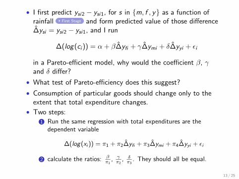
I first predict First Stage

ysi2 − ysi1, for s in {m, f , y} as a function of and form predicted value of those difference

•

rainfall Δ̂ysi = ysi2 − ysi1, and I run

Δ(log(ci )) = α + βΔ̂yfi + γΔ̂ymi + δΔ̂yyi + �i

in a Pareto-efficient model, why would the coefficient β, γ and δ differ?

• What test of Pareto-efficiency does this suggest?

• Consumption of particular goods should change only to the extent that total expenditure changes.

• Two steps: 1 Run the same regression with total expenditures are the

dependent variable

Δ(log(xi )) = π1 + π2Δ̂yfi + π3Δ̂ymi + π4Δ̂yyi + �i

γβ δ 3

2 calculate the ratios: . They should all be equal. π1 , π2

, π

13 / 25

Results Interpretation

• Results Rejection of equality of ratio

• Does not seem to be explained by obvious failure of identification

Is this a labor market failure? •

• Can this be due to lack of observability of the output?

Can this be due to moral Hazard? •

• Why do household keep separate mental account? • Incomplete contracting in the household: constant negotiations

of what transfers should be in a given period are very difficult. • Households members decide instead of very simple rules they

follow, and would be subject to strong punishment if they re-negociated upon. This allows for insurance against mis-behavior (and perhaps avoids the unpleasantness of negociating).

14 / 25

Duflo (2003)

15 / 25

Effect of the Old Age Pension Program on Weight for Height: Ordinary Least Squares andTwo-Stage Least Squares Regressions

Ordinary least squaresVariable

(1)

Girls

Eligible household

Eligible household

Woman eligible

Woman eligible

Man eligible

Man eligible

Observations

Observations

Boys

Control variables

Presence of older members

Family background variables

Child age dummy variables

* Significant at the five percent levelNote: The instruments in column 7 are woman eligible and man eligible. Standard errors (robust to correlation of residuals within house holds and heteroskedasticity) are in parentheses.

(2) (3) (4) (5) (6) (7)

Two-stageleast squares

0.14 0.35* 0.34*(0.12) (0.17) (0.17)

0.24*

(0.12)

0.61*

(0.19)

0.61*

(0.19)

1.19*

(0.41)-0.097

(0.74)

0.056

(0.19)

0.11

(0.28)

-0.011

(0.22)

0.0012

1,574 1,574 1,574 1,574 1,533 1,5331,533

(0.13)0.022(0.22)

0.030(0.24)

0.066(0.14)

0.28(0.28)

0.31(0.28)

0.58(0.53)-0.69

(0.91)

-0.25

(0.35)

-0.25

(0.34)

-0.059

(0.22)

1,670

No

No No

No

No No

Yes

Yes Yes

Yes

Yes

Yes Yes Yes

Yes Yes

Yes

Yes

Yes

Yes

Yes

1,670 1,670 1,6701,627 1,627 1,627

Figure by MIT OpenCourseWare.

Duflo (2003)

16 / 25

Effect of Pension Eligibility on Weight for Height byGender of the Intermediate Generation: Ordinary Least Squares Regressions

Variable Girls Boys

Mother's mother 0.48*

(0.21)

0.099

(0.27)0.29

(0.30)

0.15

(0.25)

0.097

(0.34)

0.00052

(0.43)

0.25

(0.44)

0.22

(0.48)

1,457 1,552

Yes

Yes

Yes

Yes

Yes

Yes

Mother's father

Father's mother

Father's father

Eligible

Eligible

Eligible

Observations

Control variables

* Significant at the five percent level.Note: Standard errors (robust to correlation of residuals withinhouseholds and heteroskedasticity) are in parentheses.

Presence of older members

Family background variables

Age dummy variables

Eligible


Duflo (2003)

17 / 25

Treatment variable

Eligibility Eligibility Oldgrandparent

Receivespension

Two-stageleast squaresOrdinary least squares

(1)

Girls

Eligible household * YOUNG0.68*(0.37)

0.71*(0.34)

0.40(0.27)

1.16*(0.56)-0.071(0.95)

-0.12(0.35)

-0.17(0.16)

-0.15(0.17)

-0.039(0.13)

-0.15(0.17)

-0.11(0.24)

1,533 1,533 1,533 1,533

-0.11(0.24)

0.027(0.15)

0.097(0.57)

Woman treatment variable * YOUNG

Man treatment variable * YOUNG

Eligible household

Woman pension variable

Man pension variable

Observations

(2) (3) (4)


Duflo (2003)

18 / 25

Height for age of children living with eligible women, eligible men, no eligible member

01/89 07/89 01/90 07/90 01/91 07/91 01/92 07/92 01/93 05/93

Date of birth

-1.5

-1

-0.5

Hei

ght f

or a

ge Z

-sco

re

Eligible woman

Eligible man

No eligible member


Thomas, Frankenberg, and Conteras (2002)

19 / 25

Impact of Parental Assets at Marriage on Child Morbidity: OLS and Fixed Effects Estimates (*100) Java and Sumatra

Sons

Paternal assets at marriage


Maternal assets at marriage


F (all covariates)

F (all covariates)

R2

R2

χ2(asset effects=0)


χ2(asset effects equal)


Cough

Fever

DaughtersDifference

OLS Fixed effects

0.135[2.60]

0.011[0.14]

0.124[1.30]

0.119[1.37]-0.236[2.78]

-0.237[1.86]

0.143[1.53]

-0.093[1.09]3.90

[0.02]1.21

[0.30]2.42

[0.09]4.73

[0.01]8.36

[0.00]4.82

[0.03]1.04

[0.31]5.08

[0.02]10.46[0.00]

0.068[0.74]

0.075[0.90]0.224[2.44]3.67

[0.03]1.29

[0.26]3.01

[0.00]

1.01[0.32]

1.20[0.30]

4.50[0.00]

0.029[0.33]0.36

[0.70]0.09

[0.77]5.50

[0.00]

0.080 0.083 0.082 0.655

-0.007[0.05]

-0.026[0.25]-0.186[2.48]3.21

[0.04]1.46

[0.23]2.53

[0.00]

-0.195[1.53]

2.60[0.00]

7.10[0.00]

2.78[0.00]0.6860.0910.0850.096

Notes: Sample size: 601 sibling pairs. Standard errors below coefficient estimates; p-values belowtest statistics. Variance-covariances matrices computed by method of infinitesimal jackknife.



20 / 25

Impact of Parental Assets at Marriage on Child Morbidity:OLS and Fixed Effects Estimates (*100)Java and Sumatra

Sons





F (all covariates)

F (all covariates)

R2

R2





Diarrhea

Other

DaughtersDifference

OLS Fixed effects

-0.002[0.03]

0.072[0.85]

-0.074[0.69]

-0.079[1.39]-0.017[0.42]

-0.024[0.43]

-0.018[0.45]

-0.042[1.13]0.64

[0.53]0.45

[0.64]0.320[0.73]

0.980[0.38]0.970[0.33]

0.170[0.68]

0.89[0.35]

0.29[0.59]2.59

[0.00]

0.066[1.05]

0.096[1.19]-0.023[0.31]0.73

[0.48]1.08

[0.30]2.52

[0.00]

0.720[0.40]

0.500[0.61]

4.570[0.00]

0.066[1.24]1.31

[0.27]0.00

[1.00]6.80

[0.00]

0.081 0.044 0.064 0.684

-0.030[0.30]

-0.063[0.61]0.110[1.57]1.340[0.26]1.750[0.19]1.910[0.00]

0.089[0.97]

1.87[0.01]

2.180[0.00]

2.030[0.00]0.6820.0670.0620.071

Notes: Sample size: 601 sibling pairs. Standard errors below coefficient estimates; p-values belowtest statistics. Variance-covariances matrices computed by method of infinitesimal jackknife.



21 / 25

Tests for Pareto Efficiency in Household Allocations Java and Sumatra Ratio of Effects of Paternal to Maternal Assets at Marriage and Non Linear Wald Tests for Equality of Ratios

Ratios of asset effects: α1/α2

Pair-wise tests for equality of ratios: χ21

Joint tests for equality of all ratios: χ25

Cough

Fever

Diarrhea

Other

-0.50

0.14

4.65

-0.57

Fever Diarrhea Other

Cough0.90

[0.14]

0.00

[0.96]1.43

[0.23]

0.41

[0.52]

1.10

[0.29]

2.52[0.77]

1.44

[0.23]

Fever

Diarrhea

Notes: P-values below test statistics. Variance-covariances matricescomputed by method of infinitesimal jackknife.


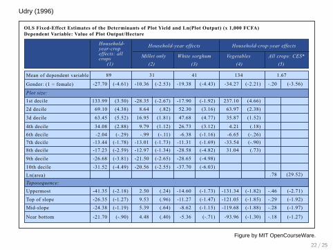
Udry (1996)

22 / 25

OLS Fixed-Effect Estimates of the Determinants of Plot Yield and Ln(Plot Output) (x 1,000 FCFA) Dependent Variable: Value of Plot Output/Hectare

Household-year-crop effects: allcrops

Household-year effects Household-crop-year effects

Millet only(1)

Mean of dependent variable

Gender: (1 = female)

Plot size:

Toposequence:

1st decile

89 31 41 134 1.67

(-3.56)

(29.52)

(-2.71)

(-1.92)(-1.97)

(-1.27)

(-2.21)

(4.66)(2.38)

(1.52)

(.18)(-.26)(-.90)(.73)

(-1.82)

(-1.85)(-1.88)

(-1.30)

(-4.43)

(-1.92)(3.16)

(4.77)

(3.12)(-1.16)(-1.69)(-4.82)

(-4.98)

(-6.03)

(-1.73)

(-1.47)

(-.71)

(-1.15)

(-2.53)

(-2.67)(.82)

(1.81)

(1.12)(-.11)

(-1.73)(-1.34)

(-2.65)

(-2.55)

(.24)

(.96)(.64)

(.40)

(-4.61) -.20

.78

-.46

-.29-.28

-.18

-34.27

237.1063.97

35.87

4.21-6.65

-33.5431.04

-131.34

-121.05-119.68

-93.96

-19.38

-17.9052.30

47.68

26.73-6.38

-11.31-28.58

-28.65

-37.70

-14.60

-11.27-8.62

-5.36

-10.36

-28.358.64

16.95

9.79-.99

-13.01-12.97

-21.50

-20.56

2.50

9.535.39

4.48

-27.70

133.99 (3.50)(4.38)

(5.52)

(2.88)(-.29)

(-1.78)(-2.59)

(-3.81)

(-4.49)

(-2.18)

(-1.27)(-1.19)

(-.90)

69.10

63.45

34.08-2.04

-13.44-17.23

-26.68

-31.52

-41.35

-26.35-24.38

-21.70

2d decile

3d decile

4th decile6th decile7th decile8th decile

9th decile

10th decileLn(area)

Uppermost

Top of slopeMid-slope

Near bottom

(2) (3) (4) (5)White sorghum Vegetables All crops: CES*


Udry (1996)

23 / 25

Least-Squares Tobit Fixed-Effect Estimates of the Determinants of Plot Input Intensities

Male laborper hectare

Female laborper hectare

Child laborper hectare

Nonhouseholdlabor per hectare

Manure (1,000)kg per hectare

Household-year-crop effects

(1)

Gender: (1 = female)

Plot size:

Toposequence:

1st decile

(-2.54)

(-.62)

(.02)

(.11)

(-.27)

(-1.70)

(.43)

(1.28)

(1.27)

(1.07)

(.80)

(.64)

(-.30)

(-.87)

(-1.07)

(.12)

(.83)

(-.11)

(.17)

(-2.34)

(1.17)

(1.11)

(1.53)

(.68)

(-.98)

(-.60)

(-1.61)

(-1.83)

(-1.86)

(-.51)

(.38)

(-1.05)

(.00)

(1.53)

(5.71)

(5.82)

(6.72)

(5.02)

(-1.36)

(-5.96)

(-6.61)

(-5.16)

(-6.08)

(-.02)

(1.07)

(.01)

(.86)

(-9.60) -16.33

-9.22

.26

1.14

2.88

-428.41

193.35

487.39

689.39

378.18

57.48

65.51

-43.81

-255.15

-220.64

(2.42)

(.96)

(.48)

(-1.12)

(-.33)

(-1.54)

(-1.61)

(-1.80)

(-2.45)

24.79

7.99

2.58

-6.18

-2.14

-11.08

-11.01

-11.64

-16.41

20.20

144.02

-15.45

23.27

-195.46

740.80

143.12

133.16

72.51

-72.15

-59.53

-184.61

-269.99

-219.27

-55.52

35.15

.10

-98.03

70.23

1,462.21

1,131.01

799.12

407.87

-69.25

-306.51

-386.78

-373.57

-418.06

-1.92

91.02

.57

75.94

-668.47

1,209.72 (2.53)

(3.25)

(2.74)

(1.71)

(-.01)

(-2.97)

(-6.23)

(-6.79)

(-7.72)

(.35)

(.30)

(.38)

(.18)

417.18

245.94

96.53

-.55

-153.12

-375.53

-413.36

-490.11

41.62

29.36

36.08

16.42

(.60)103.49

(-.85)-65.79

(-.09)-28.77

(.82)1,051.98

(1.33)274.48

(.95)196.37

(1.59)83.16

(.50)24.77

(2.57)250.40

(1.50)179.46

(.70)82.49

(1.34)78.13

(-1.84)-187.14

(1.83)95.73

(.78)35.35

(.70)19.69

427.39

506.62

(-.23)-31.68

(-.28)-30.39

(-.34)-52.06

(1.63)367.34

(-.29)-38.50

(-.49)-53.41

(.92)68.24

(-.15)-10.36

(1.36)163.76

(1.90)303.86

(.30)50.84

(-.10)-8.33

(.76)141.73

(-.33)-27.01

(.90)37.16

(.45)12.18

466.18

517.17

(.86)235.74

(.44)21.88

(-4.36)-778.86

(.44)62.36

(.35)-42.87

(2.29)205.90

(1.07)173.14

(.78)206.68

(2.60)248.38

(1.19)114.53

(1.02)79.85

(.09)42.70

(.05)2.93

(-.31)-18.82

(.93)42.92

85.55

202.88

(.50)175.29

(.47)66.04

(.70)262.71

(1.13)368.47

(-.89)-187.07

(.27)37.73

(1.00)115.56

(-.44)51.08

(-.37)-113.72

(.58)195.14

(.20)31.14

(.25)41.90

(1.27)223.23

(1.05)126.70

(-1.38)-162.88

(.30)25.80

84.88

213.11

(-1.18)-11.80

(-.01)-.07

(-.08)-.70

(1.48)16.32

(.18)2.86

(1.29)6.43

(.12).73

(1.61)17.28

(-.94)-12.75

(1.44)8.34

(1.83)8.00

(-.79)-15.45

(.17).80

(.24).99

(1.60)5.86

1.70

7.78

2d decile

3d decile

4th decile

6th decile

7th decile

8th decile

9th decile

10th decile

Uppermost

Top of slope

Mid-slope

Near bottom

Soil types:

3

7

11

12

13

21

31

32

33

35

37

45

46

51

Location:

Compound

Village

Mean of dependent variable

When > 0

(2) (3) (4) (5)

Note.- This is the least-squares implementation of Honore's (1992) fixed-effect Tobit estimator. t-ratios are in parentheses.'Figure by MIT OpenCourseWare.

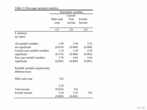
Table 2: First stage summary statistics

Male cash Yam Femalecrop income Income

(1) (2) (3)F statistics(p value)

All rainfall variables 1.99 3.50 2.53are significant (0.014) (0.000) (0.000)Current year rainfall variables 1.18 3.38 2.43significant (0.315) (0.000) (0.005)Past year rainfall variables 2.79 4.64 2.64significant (0.005) (0.000) (0.001)

Rainfall variables significantly different from:

Male cash crop NA

2.10Yam income (0.010) NAFemale income 2.10 2.38 NA

(0.009) (0.002)

Note(1) The full results are presented in Appendix, table 1(2) The specification include year dummies, region dummies, and their interactions

Dependent variablesCurrent

24 / 25

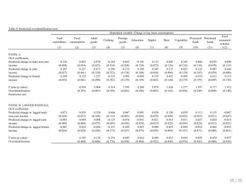
Table 4: Restricted overidentification tests

Total expenditure

Food consumption

Adult goods Clothing Prestige

goods Education Staples Meat Vegetables Processed foods

Purchased foods

Food consumed at home

(1) (2) (3) (4) (5) (6) (7) (8) (9) (10) (11) (12)

PANEL AOLS coefficients:Predicted change in male non-yam 0.126 0.062 0.870 -0.164 0.683 -0.101 0.113 0.002 0.345 0.004 -0.029 0.098income (0.049) (0.054) (0.425) (0.334) (0.209) (0.128) (0.072) (0.126) (0.210) (0.139) (0.078) (0.119)Predicted change in yam 0.207 0.227 -0.473 0.296 -0.272 0.320 0.345 0.135 0.023 0.122 0.087 0.444income (0.037) (0.041) (0.320) (0.252) (0.158) (0.108) (0.054) (0.096) (0.159) (0.105) (0.059) (0.090)Predicted change in female 0.309 0.235 1.537 0.535 0.993 -0.098 0.193 0.492 0.995 0.474 0.412 0.313income (0.056) (0.061) (0.490) (0.382) (0.239) (0.159) (0.082) (0.144) (0.239) (0.159) (0.089) (0.136)

F tests (p value) : 0.934 5.064 0.514 7.595 2.260 5.870 1.824 3.277 1.397 4.777 1.912Overidentification (0.393) (0.007) (0.598) (0.001) (0.106) (0.003) (0.162) (0.038) (0.248) (0.009) (0.148)Restriction test

PANEL B: LAGGED RAINFALLOLS coefficients: Predicted change in lagged male 0.073 0.039 0.350 0.044 0.047 0.091 0.038 0.150 0.039 0.115 0.155 -0.007non-yam income (0.020) (0.022) (0.169) (0.133) (0.082) (0.056) (0.029) (0.050) (0.083) (0.055) (0.031) (0.047)Predicted change in lagged yam -0.003 0.004 0.008 -0.125 -0.076 -0.031 -0.021 0.015 0.011 0.027 0.024 -0.018income (0.009) (0.009) (0.073) (0.059) (0.036) (0.029) (0.013) (0.022) (0.036) (0.024) (0.013) (0.021)Predicted change in lagged female -0.001 0.018 -0.024 -0.251 -0.289 0.093 0.044 0.023 -0.054 -0.010 0.062 -0.035income (0.026) (0.028) (0.220) (0.173) (0.107) (0.079) (0.038) (0.064) (0.107) (0.071) (0.040) (0.061)

F tests (p value) : 0.105 0.128 0.254 0.043 0.016 0.049 0.052 0.024 0.058 0.054 0.057Overidentification (0.900) (0.880) (0.776) (0.958) (0.984) (0.952) (0.949) (0.976) (0.943) (0.948) (0.945)Restriction testNote: The table presents the OLS coefficient of the difference in log consumption of each item on the difference in predicted log income (obtained from the equation presented in table A1). Standard errors are shown in parentheses. The regressions include year dummies, region dummies, and their interactions.The overidentification test is a non-linear wald test for the hypothesis that the coefficients in each regression are proportionalto their coefficients in column (1)

Dependent variable: Change in log (item consumption)

25 / 25

14.771 Development Economics: Microeconomic … marriage (e.g. random allocation of CCT transfers to...

Documents

Transcript of 14.771 Development Economics: Microeconomic … marriage (e.g. random allocation of CCT transfers to...