Olaf Trygve Berglihn - NTNU · Olaf Trygve Berglihn Dynamic simulation ... model in gPROMS ... α...
121
Olaf Trygve Berglihn Dynamic simulation on a thermodynamic canonical basis Doctoral thesis for the degree of philosophiae doctor Trondheim, June 2010 Norwegian University of Science and Technology Faculty of Natural Sciences and Techology Department of Chemical Engineering
Transcript of Olaf Trygve Berglihn - NTNU · Olaf Trygve Berglihn Dynamic simulation ... model in gPROMS ... α...
Olaf Trygve Berglihn
Dynamic simulationon a thermodynamiccanonical basis
Doctoral thesisfor the degree of philosophiae doctor
Trondheim, June 2010
Norwegian University of Science and TechnologyFaculty of Natural Sciences and TechologyDepartment of Chemical Engineering
NTNU
Norwegian University of Science and Technology
Doctoral thesisfor the degree of philosophiae doctor
Faculty of Natural Sciences and TechologyDepartment of Chemical Engineering
c© 2010 Olaf Trygve Berglihn.
ISBN 978-82-471-2231-0 (printed version)ISBN 978-82-471-2235-8 (electronic version)ISSN 1503-8181
Doctoral theses at NTNU, 2010:132
Printed by Tapir Uttrykk
Acknowledgments
This thesis is a contribution to the field of chemical engineering and model-ing from a thermodynamic perspective. But as in all aspects of science, thiswork would never have been possible without the work of others. And assuch, I am humble to have been given the possibility of exploring the fieldfrom the elevated perspective standing on the shoulders of giants.
First and foremost, I would like to thank my main supervisor AssociateProfessor Tore Haug-Warberg for having faith in me and opening my eyes tothe world of pure thermodynamics, not obfuscated by mundane engineeringand applied perspectives only. Professor Heinz Preisig and Professor TerjeHertzberg also deserve special thanks for their valuable input and criticalcomments.
When this work started, the thermodynamic models used were tediouslycoded by hand. If not for the work of Ph.D. Bjørn Tore Løvfall on gradi-ents of thermodynamic potentials, the development of the methods in thisthesis would have been tremendously impeded by the implementation costassociated with the thermodynamic models. Thanks, Bjørn Tore, for ourmany debates and for help with proofreading the thesis.
I would also like to thank my co-worker through these years of Ph.D.-studies, Jens Petter Strandberg for his good spirit and encouragement.Ph.D. Tarek Ali Yousef deserves his thanks for the many interesting andlengthy theoretical debates, and for help with proofreading the thesis.
Finally I would like to thank my family, my spouse Berit, and especiallymy two small kids Una and Sondre for their patience and support throughthese years. Without you, this thesis would never have been completed.
Financial support for this project was provided by The Norwegian Re-search Council, Statoil AS, Yara AS, and The Chemical Engineering De-partment, NTNU.
i

ii
Summary
In this thesis a general approach is outlined for the modeling and simula-tion of dynamic processes involving phase and reaction equilibria. A newmethodology is presented that exploits the intrinsic structure of thermody-namic functions in their canonical form.
The equations for the equilibrium sub-problems of the dynamic pro-cess are stated such as to get a mathematical problem with linear con-straints. This implies iterating in the variables most suited for the prob-lem. A methodology is given by an equation structure called the dynamicNewton-Lagrange-Euler formulation. The equation structure is a set of lin-ear equations that when solved yield a simultaneous integration in time anditeration towards the equilibrium of each sub-problem.
A software tool has been designed and implemented in order to automatethe construction and updating of the dynamic Newton-Lagrange-Euler equa-tions. Two case studies are shown that explore the described methodology.The simulation results are on par with the results found in the literature.
This systematic approach to the process modeling of flow sheets on acanonical thermodynamic basis has some promising benefits compared totraditional approaches based on a single choice of iteration variables. Thepresented methodology and software design is very general and has thepotential for wide application in dynamic simulation and the developmentof simulation software.
iii

iv
Contents
Acknowledgments i
Summary iii
Nomenclature xi
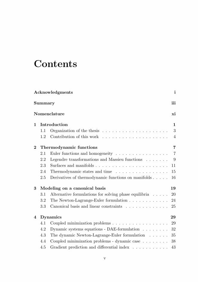
1 Introduction 1
1.1 Organization of the thesis . . . . . . . . . . . . . . . . . . . . 3
1.2 Contribution of this work . . . . . . . . . . . . . . . . . . . . 4
2 Thermodynamic functions 7
2.1 Euler functions and homogeneity . . . . . . . . . . . . . . . . 7
2.2 Legendre transformations and Massieu functions . . . . . . . 9
2.3 Surfaces and manifolds . . . . . . . . . . . . . . . . . . . . . . 11
2.4 Thermodynamic states and time . . . . . . . . . . . . . . . . 15
2.5 Derivatives of thermodynamic functions on manifolds . . . . . 16
3 Modeling on a canonical basis 19
3.1 Alternative formulations for solving phase equilibria . . . . . 20
3.2 The Newton-Lagrange-Euler formulation . . . . . . . . . . . . 24
3.3 Canonical basis and linear constraints . . . . . . . . . . . . . 25
4 Dynamics 29
4.1 Coupled minimization problems . . . . . . . . . . . . . . . . . 29
4.2 Dynamic systems equations - DAE-formulation . . . . . . . . 32
4.3 The dynamic Newton-Lagrange-Euler formulation . . . . . . 35
4.4 Coupled minimization problems - dynamic case . . . . . . . . 38
4.5 Gradient prediction and differential index . . . . . . . . . . . 43
v
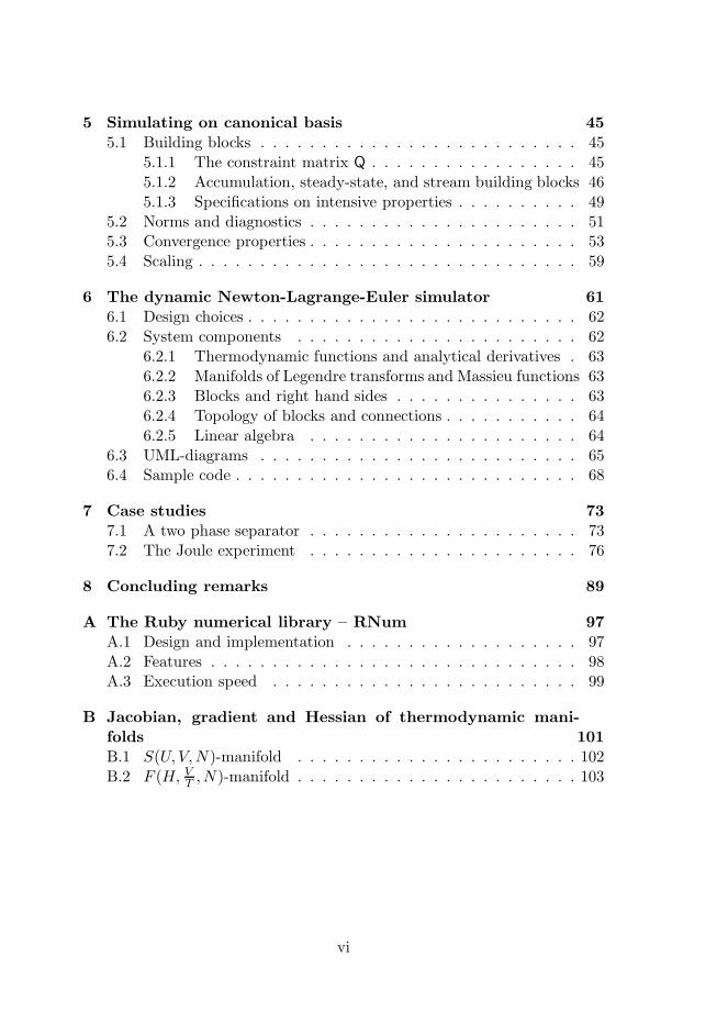
5 Simulating on canonical basis 455.1 Building blocks . . . . . . . . . . . . . . . . . . . . . . . . . . 45
5.1.1 The constraint matrix Q . . . . . . . . . . . . . . . . . 455.1.2 Accumulation, steady-state, and stream building blocks 465.1.3 Specifications on intensive properties . . . . . . . . . . 49
5.2 Norms and diagnostics . . . . . . . . . . . . . . . . . . . . . . 515.3 Convergence properties . . . . . . . . . . . . . . . . . . . . . . 535.4 Scaling . . . . . . . . . . . . . . . . . . . . . . . . . . . . . . . 59
6 The dynamic Newton-Lagrange-Euler simulator 616.1 Design choices . . . . . . . . . . . . . . . . . . . . . . . . . . . 626.2 System components . . . . . . . . . . . . . . . . . . . . . . . 62
6.2.1 Thermodynamic functions and analytical derivatives . 636.2.2 Manifolds of Legendre transforms and Massieu functions 636.2.3 Blocks and right hand sides . . . . . . . . . . . . . . . 636.2.4 Topology of blocks and connections . . . . . . . . . . . 646.2.5 Linear algebra . . . . . . . . . . . . . . . . . . . . . . 64
6.3 UML-diagrams . . . . . . . . . . . . . . . . . . . . . . . . . . 656.4 Sample code . . . . . . . . . . . . . . . . . . . . . . . . . . . . 68
7 Case studies 737.1 A two phase separator . . . . . . . . . . . . . . . . . . . . . . 737.2 The Joule experiment . . . . . . . . . . . . . . . . . . . . . . 76
8 Concluding remarks 89
A The Ruby numerical library – RNum 97A.1 Design and implementation . . . . . . . . . . . . . . . . . . . 97A.2 Features . . . . . . . . . . . . . . . . . . . . . . . . . . . . . . 98A.3 Execution speed . . . . . . . . . . . . . . . . . . . . . . . . . 99
B Jacobian, gradient and Hessian of thermodynamic mani-folds 101B.1 S(U, V,N)-manifold . . . . . . . . . . . . . . . . . . . . . . . 102B.2 F (H, V
T , N)-manifold . . . . . . . . . . . . . . . . . . . . . . . 103
vi
List of Figures
2.1 Legendre transform as tangent envelope. . . . . . . . . . . . . 10
2.2 From model to manifold . . . . . . . . . . . . . . . . . . . . . 11
2.3 Transformation from a thermodynamic surface to a thermo-dynamic manifold. . . . . . . . . . . . . . . . . . . . . . . . . 14
2.4 Change in time of thermodynamic state by explicit vs. im-plicit integration . . . . . . . . . . . . . . . . . . . . . . . . . 16
4.1 Simple steady state process with mass connection . . . . . . . 30
4.2 Snamprogetti urea-process (with courtesy of Volker Siepmann). 32
4.3 An isolated system of two gas tanks – mimicking the Jouleexperiment of 1843. . . . . . . . . . . . . . . . . . . . . . . . . 39
5.1 Connecting from a steady-state block . . . . . . . . . . . . . . 48
5.2 Connecting from an accumulation block . . . . . . . . . . . . 49
5.3 Vapor-liquid separator base case . . . . . . . . . . . . . . . . 55
5.4 Vapor-liquid separator base case with initial ∆t = 100s, re-duced by a factor
√10. . . . . . . . . . . . . . . . . . . . . . . 56
5.5 Vapor-liquid separator, with feed and product streams set to1% at time t = 5000s. . . . . . . . . . . . . . . . . . . . . . . 57
5.6 Vapor-liquid separator, with both liquid product draw set to300% at time t = 5000s. . . . . . . . . . . . . . . . . . . . . . 58
6.1 Class diagram for the Manifold . . . . . . . . . . . . . . . . . 65
6.2 Class inheritance diagram for the different block types . . . . 66
6.3 Class diagram for the Topology . . . . . . . . . . . . . . . . . 67
6.4 Components overview and interfaces . . . . . . . . . . . . . . 68
7.1 Dynamic separator with feeding reservoir and product streams. 74
7.2 Block structure for the dynamic two phase separator . . . . . 75
7.3 Composition profiles for the separator case . . . . . . . . . . 77
7.4 Temperature profile for the separator case . . . . . . . . . . . 78
vii
7.5 Pressure profile for the separator case . . . . . . . . . . . . . 787.6 Pressure profiles for the separator at selected ∆t and from a
model in gPROMS R©. . . . . . . . . . . . . . . . . . . . . . . 797.7 Block structure for the Joule case. . . . . . . . . . . . . . . . 837.8 Simulation results for the Joule case . . . . . . . . . . . . . . 857.9 Mach number for the Joule case. . . . . . . . . . . . . . . . . 86
viii
List of Tables
3.1 Thermodynamic state functions . . . . . . . . . . . . . . . . . 27
5.1 Diagnostic norms . . . . . . . . . . . . . . . . . . . . . . . . . 535.2 Scaling of units for a typical vapor and liquid using the Peng-
Robinson equation of state. . . . . . . . . . . . . . . . . . . . 59
7.1 Initial conditions for separator simulation . . . . . . . . . . . 767.2 Description of the diagonal blocks for the Joule case. . . . . . 827.3 Initial conditions for the Joule-case . . . . . . . . . . . . . . . 84
ix

x
Nomenclature
Greek letters
µ Chemical potential
α Slack variable introduced for overspecified systems of equations.
α Vapor phase mole fraction
γi Activity coefficient
φi Fugacity coefficient
ρ Density
k Iteration counter
Latin letters
h Heat transfer coefficient
H Hessian
g Gradient
H Enthalpy
Nc The number of chemical components (species).
p Pressure
t Time
Ff Feed flow rate – mole based
Fl Liquid flow rate – mole based
Fv Vapor flow rate – mole based
xi
N Flow rate – mole-based
V Volumetric flow.
R The set of real numbers
M Thermodynamic manifold
S Thermodynamic surface
L Legendre transform
M Massieu function
A Coefficient matrix for the Newton-Lagrange-Euler equations
Q Constraint matrix for balance equations
A Helmholtz energy
a Cross sectional area
Cv Valve constant.
f(z) Valve characteristics, z being actuator position.
g Standard gravity
h Specific enthalpy
K Equilibrium constant
Ki Equilibrium constant for component i
l Liquid level
N Mole number
p(l) Pressure at liquid outlet
S Entropy
T Temperature
U Inner energy
u Specific internal energy
V Volume
xii
v Specific volume
Vt Total volume
xi Mole fraction, liquid
yi Mole fraction, vapor
zi Mole fraction, feed
Mathematical symbols
x Time differential, ∂x/∂t
x vector
T Transpose
Supersrcipts
Reference
(ω) Refers to the ω phase.
F Feed
L Liquid
V Vapor
Subsrcipts
k Iteration variable
(i,j) Matrix element or sub block indices
xiii

xiv
Chapter 1
Introduction
The study of how phenomena evolve over time in chemical unit operationsgive highly valued insights for chemical engineers. With the progress incomputing powers of modern computers, processes of great complexity anddetail can be modeled and simulated for use in design studies and controlsystem design, optimization, production planning, operator training andmore.
A simulation study can roughly be split into the tasks of:
1. Physical description.
2. Mathematical description.
3. Equation manipulation and solving using a numerical method.
4. Programming.
5. Simulation and presentation.
Preforming the above tasks involves many disciplines of science. Firstly,the physical insights of the process and the decision on which relevant phe-nomena to describe is paramount for the success of the simulation study.Secondly, knowledge of both mathematical modeling and numerical methodsis required to formulate an algorithm that can be implemented. Program-ming requires yet another set of capabilities, especially for complex modelsand large systems. At last, if all the prior subtasks have been completedsuccessfully, the simulation can be run and the results disseminated usingphysical and systems insight.
For other than simple modeling and simulation, the proficiency requiredin all these disciplines exceeds the skills of the average undergraduate chem-
1
2 Introduction
ical engineer. Even at graduate level, people mastering both modeling andsimulation will usually belong to a specialized group of chemical engineers.
Several initiatives have been taken to lessen the requirements on skillsfor engaging in modeling and simulation studies. Commercial packages suchas Aspen Plus R© and Hysys R©, PRO-II R©, ProSimPlus R© and others offer thechemical engineer graphical user interfaces which hide most of the detailsof modeling and numerics for the user. Other tools, such as gPROMS R©,Ascend [Allan, 1997] and Jacobian R©, offer an input language that resemblesthe mathematical representation, and will automatically do equation re-arrangement and solve the system numerically.
However, none of the above tools are problem free. From an academicpoint of view, one would like to know what exactly is happening “under thehood” of the commercial simulators – something that is often impossibledue to the proprietary nature of these products. Moreover, the user shouldalways be able to analyze the problems arising from the choice of equationstructure and numerical strategy when the equation oriented tools are used.
For most chemical engineering problems involving rigorous phase equi-libria and reactions in dynamic simulation, the equations can be put intothe form of an Differential Algebraic Equation system (DAE):
f(x, x, y, t) = 0. (1.1)
Much work has been done over the last three decades to develop meth-ods and codes for solving this class of problems. Some of the known toolsare DASSL [Brenan et al., 1989] and various other derived implementations(Matlab R© ode15s/ode15i, Sundials Suite IDA [Hindmarsh et al., 2005], etc).Though these codes show great merit, they still only solve a subset of prob-lems (index 1-2), and depend on the equation system being well formed,and on an appropriate choice of initial values.
An alternative to solving the complete DAE is to integrate each sub-process separately by a dynamic sequential-modular scheme as shown byHlavacek [1977] and Hillestad and Hertzberg [1986]. The advantage of thismethod is that each sub-process can be developed and tested separately.However, care must be taken when choosing the calculation sequence, thehandling of calculation loops by using tear streams, and controlling the steplength for stiff systems.
Instead of looking for general tools to solve specific problems, the mo-tivation for this work started off with the opposite perspective: How canspecific problems be solved with the simplest possible means, and withoutthe loss of control over the implementation and the numerical strategy? Themotivation for taking this perspective stems from the experience with sim-
1.1. Organization of the thesis 3
ulating multiphase equilibrium problems with reaction, and the observationthat most of the numerical cost associated with solving these systems stemsfrom the calculation of thermodynamic properties and solving chemical andphase equilibria. In other words: Can the knowledge of the properties ofthermodynamic functions and their equation structure lead to simpler ormaybe better ways of constructing models for simulation studies?
The condition of phase and reaction equilibrium is a frequently usedassumption when modeling chemical phenomena. A reaction and phaseequilibrium is characterized by a maximum in entropy, subject to givenenergy, volume and mass constraints. Equivalently, the equilibrium canbe described by a minimum in internal energy (subject to given entropy,volume and mass constraints), or by a minimum of Gibbs free energy (sub-ject to given constraints on temperature, pressure and mass). Many otherformulations exist, using an extremum of a thermodynamic potential withaccompanying constraints. The question that was raised above can partlybe answered by investigating how the equilibrium condition and constraintscan be described in a manner that gives the simplest possible system ofequations to solve. This imposes a certain structure on the problem. Thetopic of this thesis is the analysis of the emerging structure and how toexploit this structure when modeling and simulating dynamic systems.
1.1 Organization of the thesis
The thesis starts with a brief summary of the theory of thermodynamicfunctions in Chapter 2. Euler homogeneity and the Legendre transformare important concepts which forms the basis for defining a thermodynamicsurface and a thermodynamic manifold, respectively. An analysis of thederivatives on the surface and the manifold is given, and this is related tointegration of dynamic processes.
Chapter 3 compares three different formulations of the phase equilib-rium problem and introduces the Newton-Lagrange-Euler formulation. Theselection of an appropriate thermodynamic potential to optimize and theproblem constraints are discussed. Each thermodynamic potential has anaccompanying set of variables which give the potential in the simplest form– the canonical basis. To arrive at a simplest possible optimization prob-lem, it is argued that a canonical basis should be chosen such that theconstraints become linear. The term canonical variables is applied to thiscanonical basis.
Each equilibrium problem can be viewed as a node. Nodes that exchangemass and energy compromise a process. A methodology for exchanging mass
4 Introduction
and energy between different nodes is given in Chapter 4. The chapter startsby looking at the steady-state case, and progresses to the dynamic case byfirst reviewing the formulation of a differential algebraic equation set (DAE).Based on the idea of using canonical variables, a formulation is given thatuse the structure of the thermodynamic equations to state the dynamic casein the Newton-Lagrange-Euler formulation. The chapter concludes with abrief discussion on the DAE index problem.
In Chapter 5 the dynamic Newton-Lagrange-Euler formulation is de-scribed in detail. The construction and update of the system of equationsare shown for phase equilibrium, both with and without reaction equilib-rium. It is also shown how to add constraints on intensive quantities, e.g.quantities that are not affected by system size; by fixing Lagrange multi-pliers. Normed quantities for step length algorithms and diagnostics aresuggested, and the convergence properties are analyzed by means of anexample. A simple scaling of the physical units is suggested for achievinggood conditioning of the Newton-Lagrange-Euler equations, without havingto rewrite the equations.
A tool has been developed for automating the construction and updat-ing of the Newton-Lagrange-Euler equations for an arbitrary set of nodes.Chapter 6 describes the design and implementation of this tool and givesan example of its use.
Finally, the methodology presented in this thesis has been applied totwo case studies given in Chapter 7. The first case study looks at a sim-ple dynamic flash model found in the literature. The model has been re-implemented using the dynamic Newton-Lagrange-Euler method and theresults compare favorably with the original paper. The second case studypresents a model of the famous Joule experiment from 1843 with a blow-down from a high pressure reservoir to a lower pressure reservoir. Simula-tions are preformed for the Joule experiment both with and without reactionequilibrium. The model includes the restriction of choked flow in the valvebetween the two reservoirs. The results are discussed.
1.2 Contribution of this work
The philosophy behind the perspective taken in this thesis builds, to a largeextent, on the work by Haug-Warberg [1988], Brendsdal [1999] and Siep-mann [2006]. The main new contributions lies in expanding on the basisfrom these authors and applying the results in the modeling and simulationof dynamic systems.
The analysis of the canonical basis and distinguishing between explicit
1.2. Contribution of this work 5
and implicit thermodynamic functions guides the understanding of the chal-lenges involved in the calculation of reaction and phase equilibria. Thedistinction is formalized by introducing the concept of a thermodynamicsurface and a thermodynamic manifold. With the choices available for ther-modynamic manifolds, a manifold can be chosen such that it best suits themodel balance equations and constraints. This leads to the definition of thecanonical basis that yields a linearly constrained problem: the canonicalvariables.
A new methodology is developed for simultaneous integration and iter-ation of phase and reaction equilibrium problems based on canonical vari-ables. This method is called the dynamic Newton-Lagrange-Euler formula-tion. The method is capable of simulating the complete process formed bya set of equilibrium nodes that exchange mass and energy. A framework forconstructing and updating the equations for the dynamic Newton-Lagrange-Euler formulation is given.
To explore the new methodology, a software tool has been designed andimplemented to automate the construction and updating of the equations.

6 Introduction
Chapter 2
Thermodynamic functions
Thermodynamic potentials are mathematical expressions that aim to de-scribe the thermodynamic properties of a collection of interacting particles.The collection, or ensemble, is described by averaging the properties of theindividual particles over time or space. The thermodynamic potential is ascalar function that take the form f : R
Nc+2 7→ R, where Nc ≥ 1 is thenumber of chemical species in the mixture. A thermodynamic potential isa state function. This implies that the function value of f for a system de-pends only on its Nc + 2 free variables, not on the way in which the systemacquired the state.
This chapter investigates the properties of thermodynamic potentialsand the use of the Legendre transform to arrive at alternative thermody-namic potentials with different sets of free variables. The concepts of thethermodynamic surface and the thermodynamic manifold are introduced todistinguish the explicitly and implicitly defined thermodynamic potentials.Methods are shown for approximating the mapping from a thermodynamicmanifold to another thermodynamic manifold or surface, and the relevanceto integration in time on a thermodynamic manifold is discussed.
2.1 Euler functions and homogeneity
The treatment of thermodynamic potentials is greatly simplified by the factthat they are linear along every straight line passing through the origin.The function f is Euler homogeneous in the variables xi, . . . , xn to degree
7
8 Thermodynamic functions
k if it satisfies the following relations
F =f(X1, . . . ,Xn, ξn+1, . . . , ξm)
=λkf(x1, . . . , xn, ξn+1, . . . , ξm), (2.1)
Xi=λxi. (2.2)
The function F is a scaling of the function f with the factor λk whenthe variables xi are scaled by a factor λ. The remaining variables, or pa-rameters, ξi are not taking part in the scaling and are thus regarded asconstants. A thermodynamic quantity is said to be extensive if the thermo-dynamic potential is Euler homogeneous to degree k = 1, and intensive ifthe state function is Euler homogeneous to degree k = 0. Scaling all exten-sive quantities by a factor λ will scale the potential accordingly. Examples ofextensive quantities are mole number and volume, and generally any otherquantity concerning the system size. Intensive quantities are independentof the system size, such as pressure and temperature.
The total differential of F can be written as follows by substituting thetotal differential dX by dX = λdx + xdλ:
dF =
(∂F
∂X
)
ξ
dX +
(∂F
∂ξ
)
X
dξ (2.3)
=
(∂F
∂X
)
ξ
xdλ +
(∂F
∂X
)
ξ
λdx +
(∂F
∂ξ
)
X
dξ. (2.4)
An alternative formulation using F = λkf yields:
dF = kλk−1fdλ + λkdf (2.5)
= kλk−1fdλ + λk
(∂f
∂x
)
ξ
dx + λk
(∂f
∂ξ
)
x
dξ. (2.6)
By comparing equivalent differentials in the Equations (2.4) and (2.6), andusing the definitions in equations (2.1) and (2.2), the following three prop-erties are found:
dλ :
(∂F
∂X
)
ξ
X = kF. (2.7)
dx :
(∂F
∂X
)
ξ
= λk−1
(∂f
∂x
)
ξ
. (2.8)
dξ :
(∂F
∂ξ
)
X
= λk
(∂f
∂ξ
)
x
. (2.9)
2.2. Legendre transformations and Massieu functions 9
Using the result in equation (2.7) for k = 1, the general integral of F hasthe solution
F (X, ξ) =
∫
(dF )ξ =
∫ (∂F
∂X
)
ξ
dX =∂F
∂X·X. (2.10)
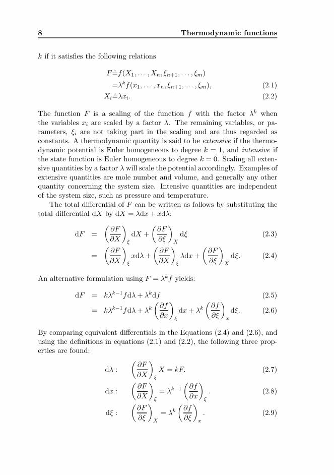
This is the Euler integration on F and is described as Euler’s first theorem.An implication of this result is that for a function of all extensive variables(k = 1) the curvature ∂2f/(∂x ∂xT ) is always zeros in the direction of x:
∂f
∂xx = f ⇒
(∂2f
∂x∂xT
)
x = 0. (2.11)
Equation (2.11) forms a part of the background for developing the methodsin this thesis, as will be discussed in Section 3.2.
2.2 Legendre transformations and Massieu func-
tions
A function f : x 7→ f(x) can be described by different functions, whoseargument is the derivative of f , rather than the function argument x, bymeans of a Legendre transform. Given f , the new function f⋆ is defined as
f⋆ : ξ 7→ f⋆(ξ) = minx
(f(x)− ξx) (2.12)
This is the general Legendre transform, L [Arnold, 1989]. For a convexfunction, the minimum f⋆ is found when ξ = ∂f(x)/∂x. In the general casein thermodynamics, the Legendre transform can be written as
f⋆i (ξi, xj , . . . , xn) = fi(xi, xj , . . . , xn)− ξixi
ξi =
(∂f
∂xi
)
xi,xk,...,xn
. (2.13)
The use of this transform is central in the manipulation of thermodynamicfunctions. The information content of the original function f is conservedunder the transformation, such that it is possible to get back the originalvariables by means of an inverse Legendre transform. As an example, thefunction of internal energy U as a function of (S, V,N) can be subjected toa Legendre transform with the variable S, yielding the Helmholtz energyfunction
A : (T, V,N) 7→ U − TS (2.14)
where T =
(∂U
∂S
)
V,N
10 Thermodynamic functions
Energy
U1
H1
V1
U2
H2
V2 V3
U3H3
Volume
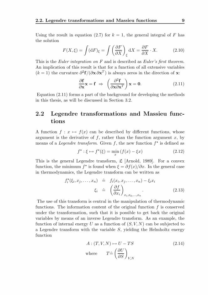
Figure 2.1: Legendre transform as tangent envelope.
or with p, yielding the enthalpy function
H : (S,−p,N) 7→ U + pV (2.15)
where p=−(
∂U
∂V
)
S,N
.
The tangent envelope of the function being transformed gives the Leg-endre transform as is shown in Figure 2.1. Starting with U1, the product ofV1 and the tangent slope −p is subtracted. This yields H1 = U1 + pV1.
In addition to the Legendre transform, swapping a variable xi with thestate function is a useful operation. The function resulting from this swap-ping is called a Massieu function of the variable xi. Massieu functions, M,are useful for expressing e.g. S(U, V,N) from U(S, V,N) and S(H, p,N)from H(S, p,N). The term Massieu function is somewhat loosely definedin the literature and is most commonly described as Legendre transformsstarting from S, rather than U [Callen, 1985].
Thermodynamic models can be categorized into two classes, dependingon the set of free variables used. Models using temperature, volume andmass as free variables are referred to as pressure explicit Equations of state,and can be viewed as a Helmholtz free energy surface A(T, V,N). Manyequations of state are able to predict both liquid and vapor properties.Models using pressure instead of volume as a free variable are generallydenoted Gibbs excess models, or activity models, and can be written as aGibbs free energy surface G(T, p,N). Activity models typically describeliquid and solid properties, and are unable, at the same time, to predict the
2.3. Surfaces and manifolds 11
Modeling(T, V, N) or (T, p, N) as independent variables
SurfacesHelmholtz (A) or Gibbs (G) free energy
ManifoldsLegendre transforms on (A) or (G)
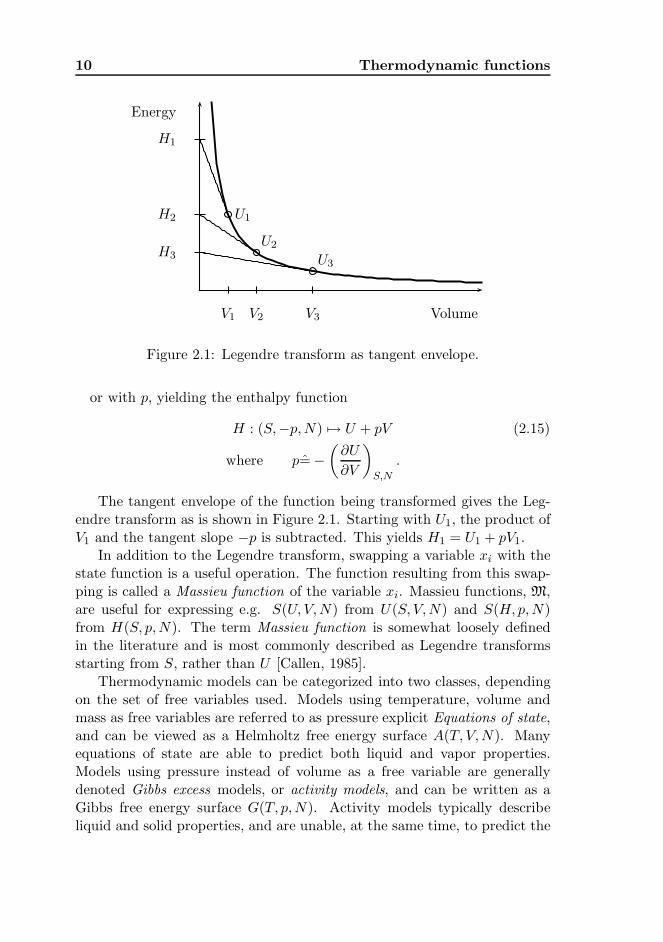
Figure 2.2: From model to manifold
properties of a vapor phase.The Helmholtz (A) or Gibbs (G) free energy surfaces can form the basis
of thermodynamic manifolds which have variables that are more convenientfor a given modeling problem. Depending on the constraints of the systembeing studied, a set of Legendre transforms can be applied in order to arriveat a manifold which has the model constrained variables as its free variables.The different set of manifold variables will be described further in Section3.3. The choice of free variables in the thermodynamic state function thusdictates the possible independent set of variables of the thermodynamicsurface, and further transformation to manifolds with different sets of in-dependent variables is possible through a series of Legendre transforms. Aschematic of the path from a thermodynamic model to a thermodynamicmanifold is shown in Figure 2.2.
2.3 Surfaces and manifolds
The following terminology will be used to describe thermodynamic poten-tials and the transformations of these:
Thermodynamic surface: The explicit thermodynamic potential, a statefunction f : R
Nc+2 → R, forms a thermodynamic surface S in RNc+2+1
.
Thermodynamic manifold: The thermodynamic surface S formed by fcan be modeled on to an Euclidean spaceM by Legendre transforms
12 Thermodynamic functions
or Massieu functions. The spaceM forms a thermodynamic manifoldin R
Nc+2+1.
According to the definitions above, the Helmholtz energy A(T, V,N) isa thermodynamic surface. From this surface the entropy S can be obtainedas a Massieu function of (U, V,N):
A : (T, V,N) 7→ A(T, V,N) (2.16)
S : (U, V,N) 7→ 1
T(U −A) =
1
T(U + pV − µN) (2.17)
using that
U = A− TS = A + T
(∂A
∂T
)
V,N
(2.18)
p = −(
∂A
∂V
)
T,N
(2.19)
µ =
(∂A
∂N
)
T,V
(2.20)
Given the coordinates [A,T, V,N ] on this thermodynamic surface S andthe partial derivatives of A at this point, the function value S(U, V,N) canbe calculated and the point [S,U, V,N ] on the thermodynamic manifoldMis found.
Now, assume changes in the internal energy, volume and mole numbersfrom [U0, V0, N0] to the new values [U1, V1, N1]. To calculate the new valueof the entropy S1 on the manifold M, the quantities 1
T1, p1 and µ1 must
be found in order to evaluate the function (2.17). Equation (2.18) musttherefore be iterated on T1 until the value for U equals U1. Then, the valueof S1 can be calculated. In other words, a point on the surface S can bemapped to a point on the manifold M. Only a single point and its localderivatives on the manifold are known. New points on the manifold canonly be found by first finding a new point on the surface S.
If gradients of A at [T0, V0, N0] are known, the gradients of S for the cor-responding values of [U0, V0, N0] can be calculated by the implicit functiontheorem. For small changes [∆U,∆V,∆N ], the gradients can be assumedconstant, and the change in S can be approximated by
dS ≈ 1
T0(dU + p0 · dV + µ0N). (2.21)
By calculating the Jacobian
J|T0,V0,N0 =∂([T, V,N ]T )
∂([U, V,N ])|T=T0,V =V0,N=N0 (2.22)
2.3. Surfaces and manifolds 13
a linear approximation of the update is given by
∆T∆V∆N
≈ J|T0,V0,N0
∆U∆V∆N
(2.23)
The transformation from a surface to a manifold will be illustrated by atrivial example. The graphical representation of a thermodynamic surfaceand the associated manifold will in general span Nc+2+1 dimensions, whichare hard to illustrate graphically. For the sake of the illustration the scopeis therefore limited to a surface of one single variable, A : T 7→ A(T ). Atransformation that will give entropy S as a function of the internal energyU is given by:
A : T 7→ A(T ) (2.24)
U = A + TS = A− T∂A
∂T(2.25)
−S =∂A
∂T(2.26)
(2.27)
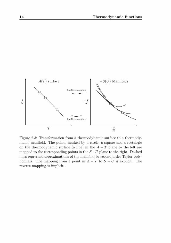
The mapping from U to −S can not be written explicitly. However, givena point [A,T ] and its derivative ∂A/∂T , the corresponding [−S,U ] canbe calculated. In order to have more information than a single point inthe S–U -plane, derivative information can be used to extrapolate along asecond order Taylor polynomial. Figure 2.3 shows a plot of the Helmholtzenergy surface using ideal gas law. The points marked with circle, squareand triangle represent three states in the Helmholtz-temperature, and thestates in the entropy-internal energy plane are given by the correspondingsymbol. The solid curve on the left represents the explicit surface. Thedashed lines on the right lines show the approximations of the manifold byTaylor-polynomials from the given points.
Assume a model is to be constructed of a closed container with fixedmass and volume, subjected to an external heat source. A typical dynamicequation to describe the flow of energy to the system is given by
U = Q = h(Ts − T ) (2.28)
where h is a heat transfer coefficient, T is the temperature in the tank, andTs is the temperature of the heat source. If the heat flow equation is inte-grated from t0 to t1 using an explicit scheme, the change in internal energyis given by ∆U = h(Ts−T |t0)∆t. This yields the update in internal energy
14 Thermodynamic functions
bc
rs
ut
AN
T
A(T ) surface
Explicit mapping
Implicit mapping
bc
rs
ut
−SN
UN
−S(U) Manifolds
Figure 2.3: Transformation from a thermodynamic surface to a thermody-namic manifold. The points marked by a circle, a square and a rectangleon the thermodynamic surface (a line) in the A − T plane to the left aremapped to the corresponding points in the S−U plane to the right. Dashedlines represent approximations of the manifold by second order Taylor poly-nomials. The mapping from a point in A − T to S − U is explicit. Thereverse mapping is implicit.
2.4. Thermodynamic states and time 15
for the container. Since only a point in the S–U -plane is known, −S1 orT1 must be found by iteration on T till the value of A and ∂A/∂T is foundthat match the updated U1, via Equation (2.25). However, extrapolationalong the Manifold given by the Taylor-expansion from the point [−S0, U0](confer with Figure 2.3), the update to [−S1, U1] can be approximated with-out iteration, and the new temperature T1 is given by the inverse gradient(∂S/∂U)−1 at [−S1, U1].
With basic knowledge of thermodynamics, this problem could be solvedusing the isochoric heat capacity Cv =
(∂U∂T
)
V,N, which is usually available
as explicit expressions if ideal gas behaviour can be assumed. The abovecase was chosen to allow for a simple and comprehensible illustration of thesurface–manifold usage and properties. For other modeling tasks, the sur-face must in general be represented in R
Nc+2+1. The strategy for updatingthe variables of the surface from the Legendre-transformed variables is thennon-trivial.
2.4 Thermodynamic states and time
There is no time associated with thermodynamic state functions. Eventhough the name is thermodynamics, time is not one of the function vari-ables, as the state is independent of the history of the system and how ithas been prepared. The dynamics behavior of the system must thereforebe explained by other factors, such as chemical reactions, flow relations,external forcing and control systems. While time is definitely relevant whenlooking at collisions and other interactions between a small set of particles,thermodynamic state functions attempt only to describe the average behav-ior of a large number of particles. However, the validity of the averagingbecomes dubious when looking at systems on a tiny scale; i.e. comparableto the mean free path of the particles.
As has been shown in this chapter, a set of Legendre transforms andMassieu functions are required to model a thermodynamic surface on to athermodynamic manifold which has variables coinciding with the dynamicmodel equations.
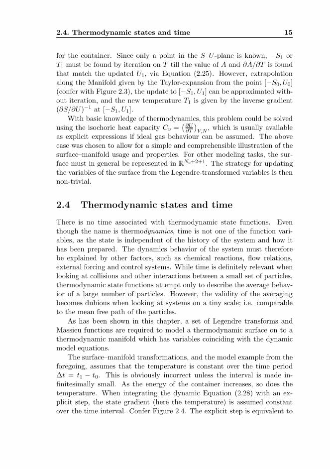
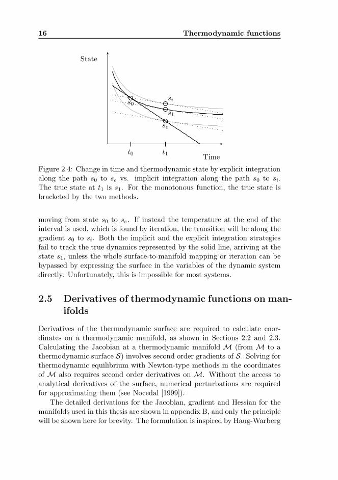
The surface–manifold transformations, and the model example from theforegoing, assumes that the temperature is constant over the time period∆t = t1 − t0. This is obviously incorrect unless the interval is made in-finitesimally small. As the energy of the container increases, so does thetemperature. When integrating the dynamic Equation (2.28) with an ex-plicit step, the state gradient (here the temperature) is assumed constantover the time interval. Confer Figure 2.4. The explicit step is equivalent to
16 Thermodynamic functions
State
Time
s0
s1
se
si
t0 t1
Figure 2.4: Change in time and thermodynamic state by explicit integrationalong the path s0 to se vs. implicit integration along the path s0 to si.The true state at t1 is s1. For the monotonous function, the true state isbracketed by the two methods.
moving from state s0 to se. If instead the temperature at the end of theinterval is used, which is found by iteration, the transition will be along thegradient s0 to si. Both the implicit and the explicit integration strategiesfail to track the true dynamics represented by the solid line, arriving at thestate s1, unless the whole surface-to-manifold mapping or iteration can bebypassed by expressing the surface in the variables of the dynamic systemdirectly. Unfortunately, this is impossible for most systems.
2.5 Derivatives of thermodynamic functions on man-
ifolds
Derivatives of the thermodynamic surface are required to calculate coor-dinates on a thermodynamic manifold, as shown in Sections 2.2 and 2.3.Calculating the Jacobian at a thermodynamic manifold M (from M to athermodynamic surface S) involves second order gradients of S. Solving forthermodynamic equilibrium with Newton-type methods in the coordinatesof M also requires second order derivatives on M. Without the access toanalytical derivatives of the surface, numerical perturbations are requiredfor approximating them (see Nocedal [1999]).
The detailed derivations for the Jacobian, gradient and Hessian for themanifolds used in this thesis are shown in appendix B, and only the principlewill be shown here for brevity. The formulation is inspired by Haug-Warberg
2.5. Derivatives of thermodynamic functions on manifolds 17
[2006]. Given an explicit thermodynamic function f and its transform f⋆
found by a combination of Legendre transforms and Massieu functions, thegradient g⋆ and Hessian are given by H⋆
g⋆ =∂f⋆
∂x⋆. (2.29)
H⋆ =∂g⋆
∂x⋆T=
∂g⋆
∂xT
∂x
∂x⋆T. (2.30)
Since dimx⋆ = dimx, the Hessian with respect to the untransformed vari-ables x can be written as
∂g⋆
∂xT=
∂g⋆
∂x⋆T
∂x⋆
∂xT. (2.31)
which leads to
H⋆ =∂g⋆
∂xT
(∂x⋆
∂xT
)−1
. (2.32)
This establishes a route from the derivatives of the thermodynamic surface,to the local derivatives of the manifold, and a Jacobian for mapping a pointon the manifold back to the surface.
The Hessian H⋆ is a second order derivative, and it follows that it mustbe symmetric. As shown in the appendix B, the Hessian can be written asa congruence product
H = αLALT . (2.33)

18 Thermodynamic functions
Chapter 3
Modeling on a canonical
basis
The term Canonical denotes the characteristic of being in its standard form,usually also the simplest form. In thermodynamics, a canonical basis givesa complete description of the thermodynamic state with no loss of informa-tion; the function U : (S, V,N) 7→ U(S, V,N) contains the same informa-tion as A : (T, V,N) 7→ A(T, V,N) [Callen, 1985]. In the previous chapter,methods for mapping from one canonical basis to another by the use of theLegendre transform and the Massieu function were shown. This chapter willfocus on the selection of sets of variables when modeling phase and reactionequilibria such that the representation is as simple as possible.
First, a review of alternative formulations for solving phase equilibriais given. It will be shown that the problem can be stated as a constrainedminimization of Gibbs Free Energy and how this formulation can solve si-multaneous phase and reaction equilibria. This leads to a general iterationscheme for solving the equilbria using any thermodynamic state function:The Newton-Lagrange-Euler formulation. The rest of this chapter deals withthe selection of a proper canonical basis, such that the constrained mini-mization problem associated with the phase and reaction equilibria will belinearly constrained. A canonical basis that achieves this property will bedefined as the canonical variables of the problem.
19
20 Modeling on a canonical basis
3.1 Alternative formulations for solving phase equi-
libria
Take as an example the steady-state flash drum. A common method for solv-ing for the equilibrium composition at constant temperature and pressureis the well established Rachford-Rice equations, also known as the K-valuemethod [Biegler, 1997]. A mass balance is written on the mass flow ratesF over the drum for each component. The mole fraction of component i inthe vapor phase, yi, is given by the scalar K-function value Ki multipliedwith the liquid mole fraction xi. Note that the K-function is a compositefunction of the activity coefficient function γi, the reference fugacity func-tion f0
i and the fugacity function φi, and thus depends on the compositionof both liquid and vapor phases, the temperature, and the pressure. TheRachford-Rice equations are given by
Ff = Fl + Fv. (3.1)
ziFf = Fvyi + Flxi (3.2)
yi = Kixi (3.3)
Ki =γi(x, T )f0
i (T, p)
φi(y, T )p. (3.4)
∑
yi −∑
xi = 0 (3.5)
which after introduction of the vapor face fraction α and some substitutionleads to
α =V
F(3.6)
f(α) =∑
yi −∑
xi =∑ (Ki − 1)zi
1 + (Ki − 1)α= 0. (3.7)
The problem can be solved by iteration with the Newton formula
αk+1 = αk −(
∂f
∂α
)−1
f. (3.8)
After converging the equation with respect to the vapor fraction α, the Ki
values must be updated, and the Newton iteration run repeatedly until nochanges in the compositions xi, yi and the Ki are observed. The Rachford-Rice method works well for mildly non-ideal mixtures, but may requirevery frequent calls to the thermodynamic functions for other cases. This isespecially true when the enthalpy balance needs to be incorporated. Also,
3.1. Alternative formulations for solving phase equilibria 21
the method becomes less intuitive for multi-phase systems, and difficult toextend to reacting mixtures.
An alternative method for solving the flash drum problem is to formulateit as an optimization problem with Nc components and α and β phases. Theobjective is to minimize the Gibbs free energy G, at which the equilibriumis found:
minN
(α)i ,N
(β)i
GT,p(N(α)i , N
(β)i ) i = 1, . . . , Nc (3.9)
subject to
N(α)i + N
(β)i = Ni. (3.10)
The solution is found when
dG =∑
i
∂G(α)i
∂N(α)i
dN(α)i +
∂G(β)i
∂N(β)i
dN(β)i =
∑
i
µ(α)i dN
(α)i + µ
(β)i dN
(β)i = 0.
(3.11)Here µi is known as the chemical potential of component i. The massbalance constraint can be written as
dN(α)i = −dN
(β)i . (3.12)
Introducing G as the second order derivatives of the Gibbs free energy andn as the vector of mole numbers Ni, the resulting Newton-Raphson formulacan then be written as
µ(α) + G(α)∆n(α) = µ(β) + G(β)∆n(β) (3.13)
−∆n(α) = ∆n(β) (3.14)
Defining ∆µ = µ(α)−µ(β) and H = G(α)+G(β), leads to the general Newtonupdate formula:
∆n(α) = −H−1∆µ (3.15)
The Newton-Raphson iteration has second order convergence and showsgood behavior in non-ideal mixtures and close to critical points. But havingfairly accurate starting points is a prerequisite, and finding these is often adifficult task. Additionally, calculating ∆µ and H requires first and secondorder derivatives of G.
A third formulation, closely linked to the Newton-Raphson scheme is thetechnique of Lagrange multipliers as known from optimization textbooks[Nocedal, 1999]. The mass balance constraint is here combined with the
22 Modeling on a canonical basis
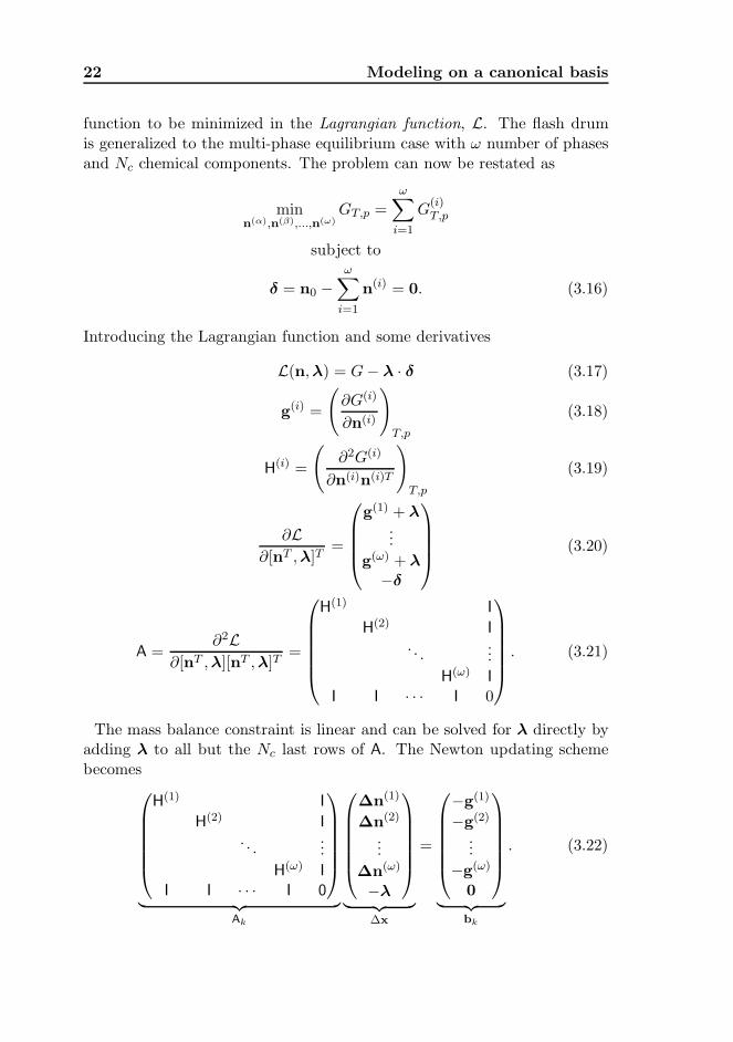
function to be minimized in the Lagrangian function, L. The flash drumis generalized to the multi-phase equilibrium case with ω number of phasesand Nc chemical components. The problem can now be restated as
minn(α),n(β),...,n(ω)
GT,p =
ω∑
i=1
G(i)T,p
subject to
δ = n0 −ω∑
i=1
n(i) = 0. (3.16)
Introducing the Lagrangian function and some derivatives
L(n,λ) = G− λ · δ (3.17)
g(i) =
(
∂G(i)
∂n(i)
)
T,p
(3.18)
H(i) =
(
∂2G(i)
∂n(i)n(i)T
)
T,p
(3.19)
∂L∂[nT ,λ]T
=
g(1) + λ...
g(ω) + λ
−δ
(3.20)
A =∂2L
∂[nT ,λ][nT ,λ]T=
H(1) I
H(2) I
. . ....
H(ω) I
I I · · · I 0
. (3.21)
The mass balance constraint is linear and can be solved for λ directly byadding λ to all but the Nc last rows of A. The Newton updating schemebecomes
H(1) I
H(2) I
. . ....
H(ω) I
I I · · · I 0
︸ ︷︷ ︸
Ak
∆n(1)
∆n(2)
...
∆n(ω)
−λ
︸ ︷︷ ︸
∆x
=
−g(1)
−g(2)
...
−g(ω)
0
︸ ︷︷ ︸
bk
. (3.22)
3.1. Alternative formulations for solving phase equilibria 23
For the one- and two-phase case, the matrix Ak is easily inverted:(
H I
I 0
)−1
=
(0 I
I −H
)
(3.23)
H1 I
H2 I
I I 0
−1
=
(H(1) + H(2))−1 −(H(1) + H(2))−1 I− (H(1) + H(2))−1H1
−(H(1) + H(2))−1 (H(1) + H(2))−1 (H(1) + H(2))−1H1
I− H1(H(1) + H(2))−1 H1(H
(1) + H(2))−1 −H2(I− (H(1) + H(2))−1H1)
(3.24)
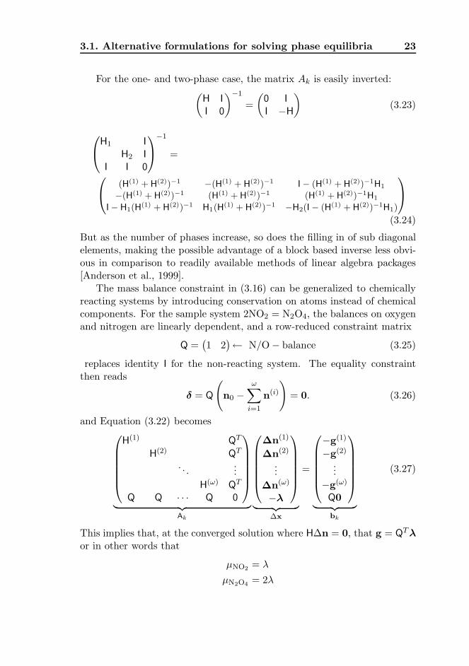
But as the number of phases increase, so does the filling in of sub diagonalelements, making the possible advantage of a block based inverse less obvi-ous in comparison to readily available methods of linear algebra packages[Anderson et al., 1999].
The mass balance constraint in (3.16) can be generalized to chemicallyreacting systems by introducing conservation on atoms instead of chemicalcomponents. For the sample system 2NO2 = N2O4, the balances on oxygenand nitrogen are linearly dependent, and a row-reduced constraint matrix
Q =(1 2
)← N/O− balance (3.25)
replaces identity I for the non-reacting system. The equality constraintthen reads
δ = Q
(
n0 −ω∑
i=1
n(i)
)
= 0. (3.26)
and Equation (3.22) becomes
H(1) QT
H(2) QT
. . ....
H(ω) QT
Q Q · · · Q 0
︸ ︷︷ ︸
Ak
∆n(1)
∆n(2)
...
∆n(ω)
−λ
︸ ︷︷ ︸
∆x
=
−g(1)
−g(2)
...
−g(ω)
Q0
︸ ︷︷ ︸
bk
(3.27)
This implies that, at the converged solution where H∆n = 0, that g = QT λ
or in other words that
µNO2 = λ
µN2O4 = 2λ
24 Modeling on a canonical basis
which in turn implies
2µNO2 = µN2O4 .
Inerts can be introduced in the n-vector to inhibit equilibrium reactionon some species, and different component lists for each phase can be used byintroducing a projection onto a common basis [Brendsdal, 1999, Siepmann,2006].
The minimization of Gibbs Free energy for solving a general, multiphasesystem was first proposed by White et al. [1958], and the methods have laterbeen extended and explored by several authors [Castillo and Grossmann,1981, Seider and Widagdo, 1996]. Computation of thermodynamic equi-librium by the iteration scheme shown in Equations (3.22) and (3.27) hasbeen reviewed and explored by Haug-Warberg [1988] and Brendsdal [1999].Although the minimization of Gibbs energy is a frequently encounteredmethodology in the literature, it is seldom used in commercial simulatorswhere the K-value method is still dominates. Few publications exist usingminimization of other energy functions. Two examples are Brendsdal [1999]and Castier [2009].
Note that phase stability is not considered here. Stability criterions andalgorithm is thoroughly described by Haug-Warberg [1988].
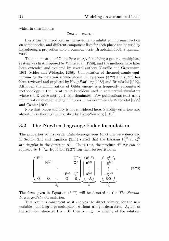
3.2 The Newton-Lagrange-Euler formulation
The properties of first order Euler-homogeneous functions were described
in Section 2.1, and Equation (2.11) stated that the Hessians H(i)k at x
(i)k
are singular in the direction x(i)k . Using this, the product H(i)∆x can be
replaced by H(i)x. Equation (3.27) can then be rewritten as
H(1) QT
H(2) QT
. . ....
H(ω) QT
Q Q · · · Q 0
︸ ︷︷ ︸
Ak
n(1)
n(2)
...
n(ω)
−λ
︸ ︷︷ ︸
x
=
−g(1)
−g(2)
...
−g(ω)
Q0
︸ ︷︷ ︸
bk
. (3.28)
The form given in Equation (3.27) will be denoted as the The Newton-Lagrange-Euler -formulation.
This result is convenient as it enables the direct solution for the newvariables and Lagrange-multipliers, without using a delta-form. Again, atthe solution where all Hn = 0, then λ = g. In vicinity of the solution,
3.3. Canonical basis and linear constraints 25
the Lagrange multipliers give a second order approximation of the k + 1gradient.
3.3 Canonical basis and linear constraints
The Newton-Lagrange formulations (3.22) and (3.27) were stated for a sys-tem constrained to constant temperature and pressure, and by mass bal-ance on component or atom basis. Other systems have other constraints.A closed container could be modeled at constant temperature and volume,or with constant volume and balance on energy and mass, or even withconstraints on the chemical potentials, rather than mass, for membranesystems.
The minimization problem associated with the choice of constraints fol-lows from the basic equations for equilibrium as shown by Callen [1985].At equilibrium, the combined system and reservoir/surroundings (r) is atminimum total energy when
d(U + U (r)) = 0 Energy conservation (3.29)
d2(U + U (r)) = d2U > 0 Minimum condition (3.30)
This is the general form of the equilibrium conditions. Note that the mini-mum condition can be stated on U only, since the second order total differ-ential with respect to the reservoir is zero:
d2U (r) =∑
j
∑
k
∂2U (r)
∂X(r)j ∂X
(r)k
dX(r)j dX
(r)k = 0. (3.31)
Different formulations of the minimization problem can be chosen basedon the system constraints. The most commonly used are stated here (fromCallen [1985]):
Helmholtz potential minimum principle. The equilib-rium value of any unconstrained internal parameter in a sys-tem in diathermal contact with a heat reservoir minimizes theHelmholtz potential over the manifold of states for which T =T (r).
Enthalpy minimum principle. The equilibrium value ofany unconstrained internal parameter in a system in contactwith a pressure reservoir minimizes the enthalpy over the mani-fold of states of constant pressure (equal to that of the pressurereservoir).
26 Modeling on a canonical basis
Gibbs potential minimum principle. The equilibriumvalue of any unconstrained internal parameter in a system incontact with a thermal and a pressure reservoir minimizes theGibbs potential at constant temperature and pressure (equal tothose of the respective reservoirs).
And this is further generalized to systems characterized by other exten-sive parameters in addition to the volume and mole numbers to yield
The general minimum principle for Legendre trans-forms of the energy. The equilibrium value of any uncon-strained internal parameter in a system in contact wth a set of
reservoirs (with intensive parameters P(r)1 , P
(r)2 , . . . ) minimizes
the thermodynamic potential LP1,P2,...[U ] at constant P1, P2, . . .
(equal to P(r)1 , P
(r)2 , . . . ).
For other thermodynamic functions, involving variable substitution, e.g.Massieu-functions, the extremal condition can be reversed. Hence the equi-librium is found for the entropy function S when d2S > 0. In general, goingfrom one formulation to another, the associated congruence transform ofthe Hessian will reveal whether the new function will have a minimum or amaximum at the equilibrium. If there is a sign change on the eigenvalues inthe congruence transform, the extremal condition flips. Some transforms ofthe Hessians are shown in appendix B.
This can be generalized even further to state the equilibrium problem inany Massieu function and set of Legendre transforms of a thermodynamicstate function. Finding the extremal value (maximum or minimum, respec-tively) of these functions will give the equilibrium value of any unconstrainedinternal parameter. If the internal parameter is also the system constrainedvariable the extremal value problem will be a linearly constrained problem.This result should be emphasized, as it is of major importance:
Given the constrained variables of the problem, seek thethermodynamic state function function that will have these con-strained variables as free variables. The optimization problem offinding the equilibrium will then have linear constraints.
Expressing the optimization problem in other variables than that ofthe explicit thermodynamic state function require the use of the Legendretransform and the Massieu function to model a manifold from an explicitthermodynamic surface. The functions from the set of possible transforms
3.3. Canonical basis and linear constraints 27
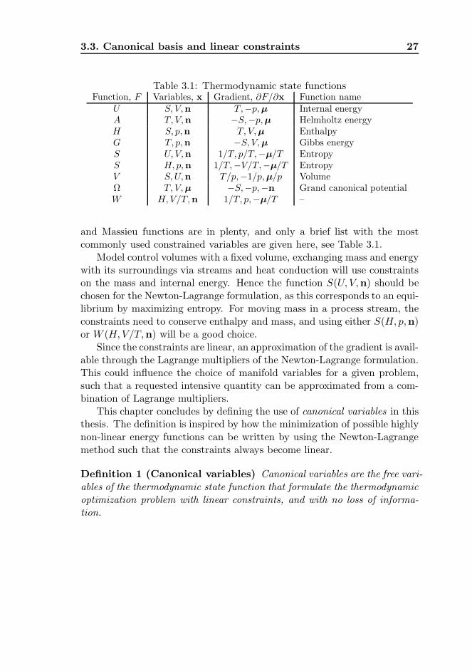
Table 3.1: Thermodynamic state functionsFunction, F Variables, x Gradient, ∂F/∂x Function name
U S, V,n T,−p, µ Internal energyA T, V,n −S,−p, µ Helmholtz energyH S, p,n T, V, µ EnthalpyG T, p,n −S, V, µ Gibbs energyS U, V,n 1/T, p/T,−µ/T EntropyS H, p,n 1/T,−V/T,−µ/T EntropyV S, U,n T/p,−1/p, µ/p VolumeΩ T, V, µ −S,−p,−n Grand canonical potentialW H, V/T,n 1/T, p,−µ/T –
and Massieu functions are in plenty, and only a brief list with the mostcommonly used constrained variables are given here, see Table 3.1.
Model control volumes with a fixed volume, exchanging mass and energywith its surroundings via streams and heat conduction will use constraintson the mass and internal energy. Hence the function S(U, V,n) should bechosen for the Newton-Lagrange formulation, as this corresponds to an equi-librium by maximizing entropy. For moving mass in a process stream, theconstraints need to conserve enthalpy and mass, and using either S(H, p,n)or W (H,V/T,n) will be a good choice.
Since the constraints are linear, an approximation of the gradient is avail-able through the Lagrange multipliers of the Newton-Lagrange formulation.This could influence the choice of manifold variables for a given problem,such that a requested intensive quantity can be approximated from a com-bination of Lagrange multipliers.
This chapter concludes by defining the use of canonical variables in thisthesis. The definition is inspired by how the minimization of possible highlynon-linear energy functions can be written by using the Newton-Lagrangemethod such that the constraints always become linear.
Definition 1 (Canonical variables) Canonical variables are the free vari-ables of the thermodynamic state function that formulate the thermodynamicoptimization problem with linear constraints, and with no loss of informa-tion.

28 Modeling on a canonical basis
Chapter 4
Dynamics
In Chapter 3, the Newton-Lagrange formulation for phase and chemicalequilibrium was introduced, in addition to the concept of canonical vari-ables for making the constraints linear. In this chapter, attention will begiven to how this formulation can be used to build a set of interconnectedminimization problems to integrate dynamic flowsheets.
4.1 Coupled minimization problems
The idea of interconnecting minimization problems has been described andused by Siepmann [2006] to model steady-state flowsheets . He also built ageneral steady-state simulatorYasim based on these techniques. The basicidea for the steady-state case is to aggregate the i individual A(i,i),k-matricesalong the block diagonal of a combined matrix Ak, and connect the i-th andj-th minimization problem by adding an off-diagonal block A(i,j).
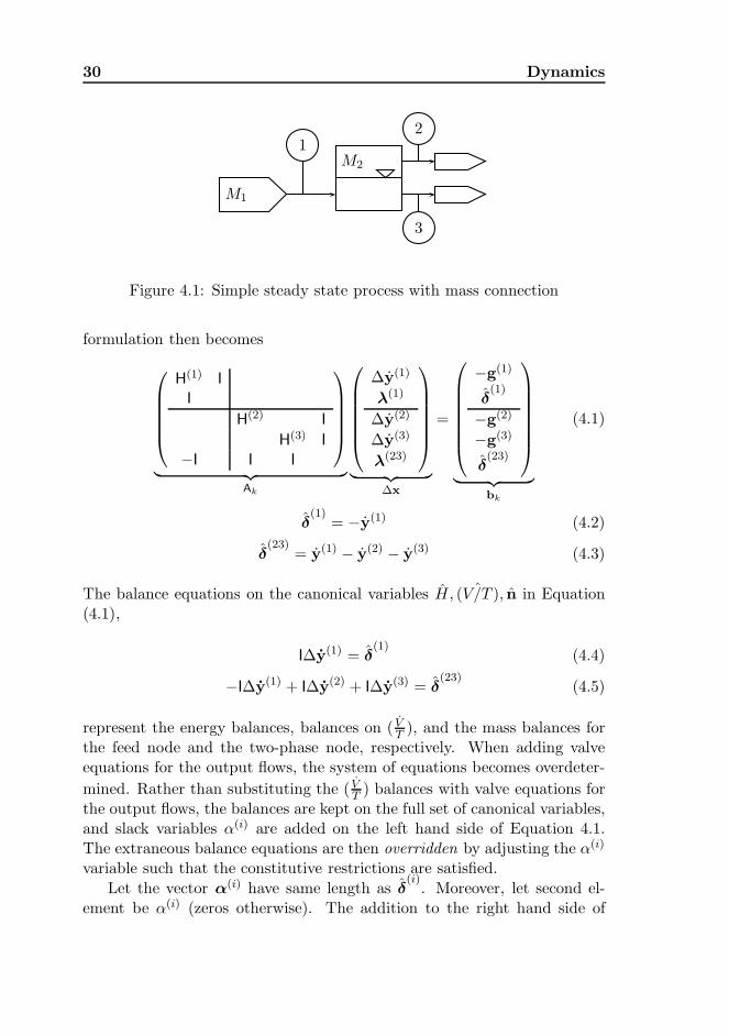
An example of the connection of minimization problems is given byconsidering the simple process in Figure 4.1. A feed stream enters a twophase separator with two exit streams. This process can be represented by asingle 1-phase equilibrium system coupled to a 2-phase equilibrium systemwith mass and energy exchange. The system is constrained by mass andenergy balances, and the volumetric flow rates are constrained to fulfill twovalve equations, typically on the form h = V 2 − C2
v∆p = 0. Here V is thevolumetric flow rate, Cv is the valve characteristic, and ∆p the pressuredifference over the valve.
With constraints on enthalpy and mass, and with flow constraints relat-
ing to the pressure, the canonical variable set y =[
H, ˙(V/T ), n]
was chosen
to get linearly constrained optimization problems. The Newton-Lagrange
29
30 Dynamics
M1
1M2
2
3
Figure 4.1: Simple steady state process with mass connection
formulation then becomes
H(1) I
I
H(2) I
H(3) I
−I I I
︸ ︷︷ ︸
Ak
∆y(1)
λ(1)
∆y(2)
∆y(3)
λ(23)
︸ ︷︷ ︸
∆x
=
−g(1)
δ(1)
−g(2)
−g(3)
δ(23)
︸ ︷︷ ︸
bk
(4.1)
δ(1)
= −y(1) (4.2)
δ(23)
= y(1) − y(2) − y(3) (4.3)
The balance equations on the canonical variables H, ˆ(V/T ), n in Equation(4.1),
I∆y(1) = δ(1)
(4.4)
−I∆y(1) + I∆y(2) + I∆y(3) = δ(23)
(4.5)
represent the energy balances, balances on ( VT ), and the mass balances for
the feed node and the two-phase node, respectively. When adding valveequations for the output flows, the system of equations becomes overdeter-
mined. Rather than substituting the ( VT ) balances with valve equations for
the output flows, the balances are kept on the full set of canonical variables,and slack variables α(i) are added on the left hand side of Equation 4.1.The extraneous balance equations are then overridden by adjusting the α(i)
variable such that the constitutive restrictions are satisfied.
Let the vector α(i) have same length as δ(i)
. Moreover, let second el-ement be α(i) (zeros otherwise). The addition to the right hand side of
4.1. Coupled minimization problems 31
Equation (4.1) can then be written as
[0,α(1),0,0,α(23)]T = E
(α(1)
α(23)
)
= Eα. (4.6)
The flow relations h, and derivatives in terms of the free variables x =[x,α]T are given by
h(x) = 0 (4.7)
Jx=
(∂h
∂xT
)
(4.8)
Jα=
(∂h
∂αT
)
. (4.9)
These equations can be iterated using the Newton method simultaneouslywith the rest of the Newton-Lagrange system of equations by augmentingthe Equation (4.1) to the fully determined
A∆x + E∆α = b + Eα
Jx∆x + Jα∆α = −h
⇓(
A E
Jx Jα
)
︸ ︷︷ ︸
Ak
(∆x∆α
)
︸ ︷︷ ︸
∆x
=
(b + Eα
−h
)
︸ ︷︷ ︸
bk
. (4.10)
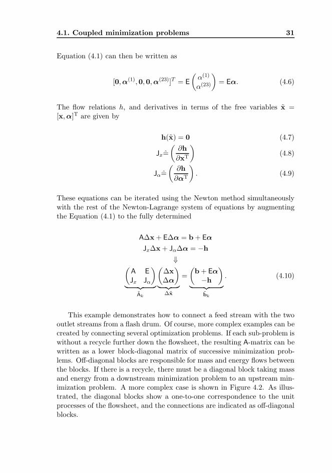
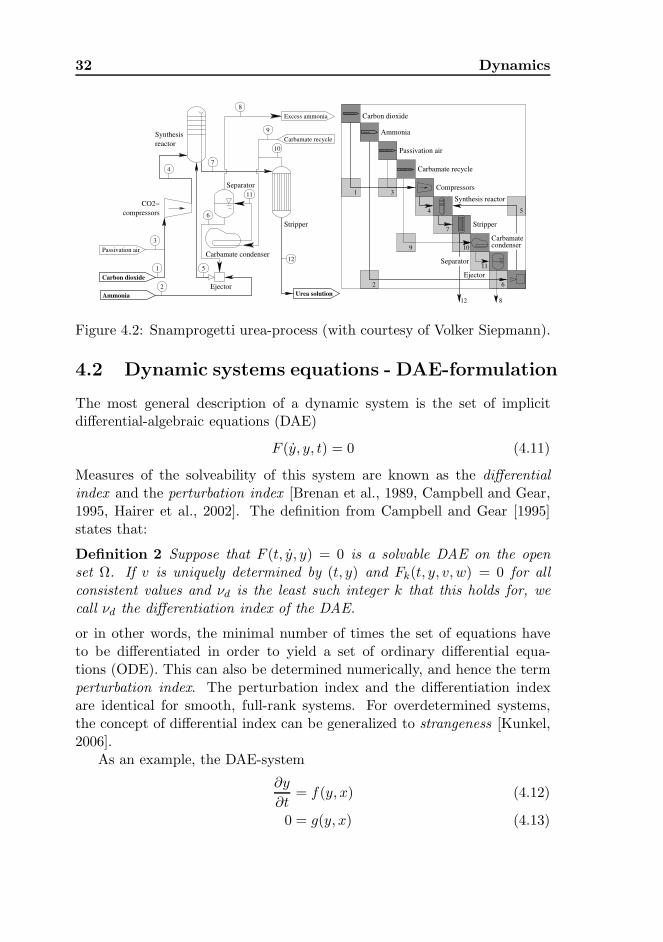
This example demonstrates how to connect a feed stream with the twooutlet streams from a flash drum. Of course, more complex examples can becreated by connecting several optimization problems. If each sub-problem iswithout a recycle further down the flowsheet, the resulting A-matrix can bewritten as a lower block-diagonal matrix of successive minimization prob-lems. Off-diagonal blocks are responsible for mass and energy flows betweenthe blocks. If there is a recycle, there must be a diagonal block taking massand energy from a downstream minimization problem to an upstream min-imization problem. A more complex case is shown in Figure 4.2. As illus-trated, the diagonal blocks show a one-to-one correspondence to the unitprocesses of the flowsheet, and the connections are indicated as off-diagonalblocks.
32 Dynamics
Carbon dioxide
Ammonia
Passivation air
Carbamate recycle
Urea solution
Excess ammonia
Ejector
Carbamate condenser
Synthesis
reactor
Separator
Stripper
compressors
CO2−
2
4
5
6
7
8
10
11
3
1
12
9
7
4
31
2
5
6
9 10
11
812
Carbon dioxide
Ammonia
Passivation air
Carbamate recycle
Carbamatecondenser
Stripper
Ejector
Synthesis reactor
Compressors
Carbamate recycle
Passivation air
Ammonia
Carbon dioxide
Separator
Figure 4.2: Snamprogetti urea-process (with courtesy of Volker Siepmann).
4.2 Dynamic systems equations - DAE-formulation
The most general description of a dynamic system is the set of implicitdifferential-algebraic equations (DAE)
F (y, y, t) = 0 (4.11)
Measures of the solveability of this system are known as the differentialindex and the perturbation index [Brenan et al., 1989, Campbell and Gear,1995, Hairer et al., 2002]. The definition from Campbell and Gear [1995]states that:
Definition 2 Suppose that F (t, y, y) = 0 is a solvable DAE on the openset Ω. If v is uniquely determined by (t, y) and Fk(t, y, v, w) = 0 for allconsistent values and νd is the least such integer k that this holds for, wecall νd the differentiation index of the DAE.
or in other words, the minimal number of times the set of equations haveto be differentiated in order to yield a set of ordinary differential equa-tions (ODE). This can also be determined numerically, and hence the termperturbation index. The perturbation index and the differentiation indexare identical for smooth, full-rank systems. For overdetermined systems,the concept of differential index can be generalized to strangeness [Kunkel,2006].
As an example, the DAE-system
∂y
∂t= f(y, x) (4.12)
0 = g(y, x) (4.13)
4.2. Dynamic systems equations - DAE-formulation 33
must be differentiated once to obtain
∂x
∂t= −
(∂g
∂x
)−1 ∂g
∂yf (4.14)
and is hence index-1. On the other hand, the DAE-system
∂y
∂t= f(y, x) (4.15)
0 = g(y) (4.16)
will give a hidden constraint when the algebraic equation is differentiatedto find
0 =∂g
∂yf (4.17)
and needs to be differentiated twice to get at system of only ODEs:
0 =∂2g
∂y2f +
∂g
∂y
∂f
∂yf +
∂g
∂y
∂f
∂x
∂x
∂t(4.18)
⇓∂x
∂t= −
(∂g
∂y
∂f
∂x
)−1(∂2g
∂y2f +
∂g
∂y
∂f
∂yf
)
. (4.19)
Hence, this system is index-2. Available DAE-codes will in general be unableto cope with systems of differential index higher than 1.
Index-1 formulations of chemical engineering problems can be writtenon the following form:
x(t) =
∫ t
t0
x dt + x(t0) (4.20)
x = Fz (4.21)
f : y 7→ z (4.22)
g(x,y) = 0 (4.23)
Solving this system with available DAE-methods will involve a discretizationin time to solve a large system of equations simultaneously. The systemalso has to be given consistent initial conditions. For systems involvingthermodynamic equilibria, the set of equations (4.23) can be highly non-linear.
The DAE formulation of the simple example shown in Figure 4.1 can bewritten as
34 Dynamics
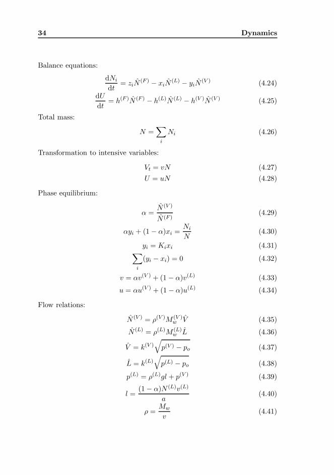
Balance equations:
dNi
dt= ziN
(F ) − xiN(L) − yiN
(V ) (4.24)
dU
dt= h(F )N (F ) − h(L)N (L) − h(V )N (V ) (4.25)
Total mass:
N =∑
i
Ni (4.26)
Transformation to intensive variables:
Vt = vN (4.27)
U = uN (4.28)
Phase equilibrium:
α =N (V )
N (F )(4.29)
αyi + (1− α)xi =Ni
N(4.30)
yi = Kixi (4.31)∑
i
(yi − xi) = 0 (4.32)
v = αv(V ) + (1− α)v(L) (4.33)
u = αu(V ) + (1− α)u(L) (4.34)
Flow relations:
N (V ) = ρ(V )M (V )w V (4.35)
N (L) = ρ(L)M (L)w L (4.36)
V = k(V )√
p(V ) − po (4.37)
L = k(L)√
p(L) − po (4.38)
p(L) = ρ(L)gl + p(V ) (4.39)
l =(1− α)N (L)v(L)
a(4.40)
ρ =Mw
v(4.41)
4.3. The dynamic Newton-Lagrange-Euler formulation 35
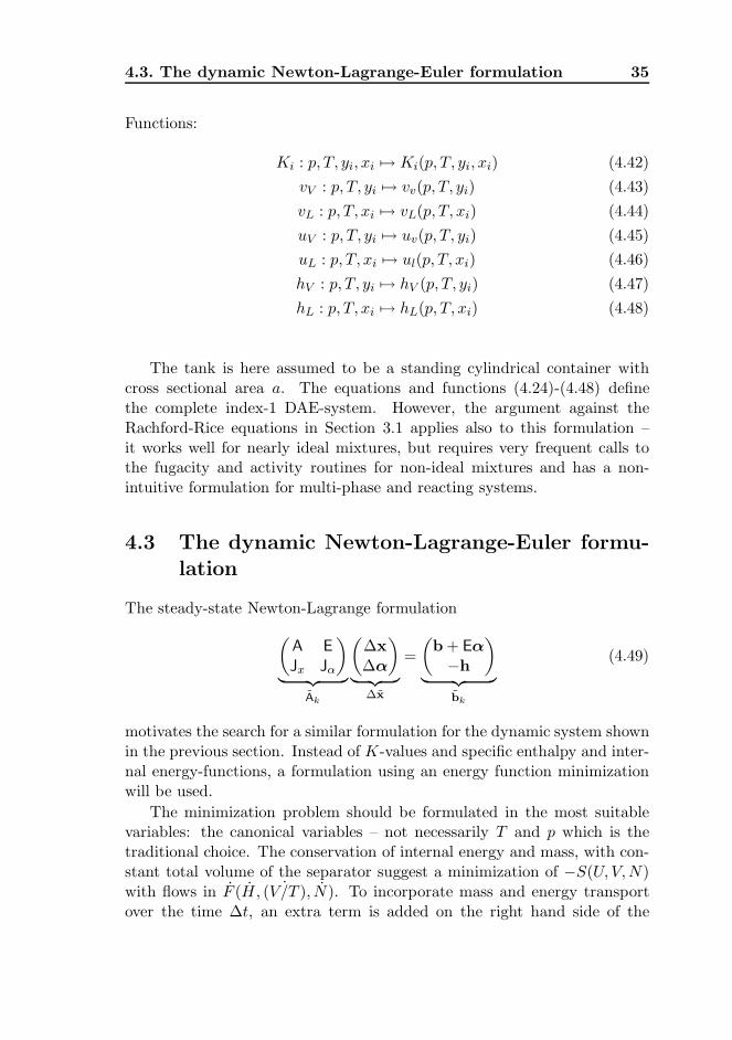
Functions:
Ki : p, T, yi, xi 7→ Ki(p, T, yi, xi) (4.42)
vV : p, T, yi 7→ vv(p, T, yi) (4.43)
vL : p, T, xi 7→ vL(p, T, xi) (4.44)
uV : p, T, yi 7→ uv(p, T, yi) (4.45)
uL : p, T, xi 7→ ul(p, T, xi) (4.46)
hV : p, T, yi 7→ hV (p, T, yi) (4.47)
hL : p, T, xi 7→ hL(p, T, xi) (4.48)
The tank is here assumed to be a standing cylindrical container withcross sectional area a. The equations and functions (4.24)-(4.48) definethe complete index-1 DAE-system. However, the argument against theRachford-Rice equations in Section 3.1 applies also to this formulation –it works well for nearly ideal mixtures, but requires very frequent calls tothe fugacity and activity routines for non-ideal mixtures and has a non-intuitive formulation for multi-phase and reacting systems.
4.3 The dynamic Newton-Lagrange-Euler formu-
lation
The steady-state Newton-Lagrange formulation
(A E
Jx Jα
)
︸ ︷︷ ︸
Ak
(∆x∆α
)
︸ ︷︷ ︸
∆x
=
(b + Eα
−h
)
︸ ︷︷ ︸
bk
(4.49)
motivates the search for a similar formulation for the dynamic system shownin the previous section. Instead of K-values and specific enthalpy and inter-nal energy-functions, a formulation using an energy function minimizationwill be used.
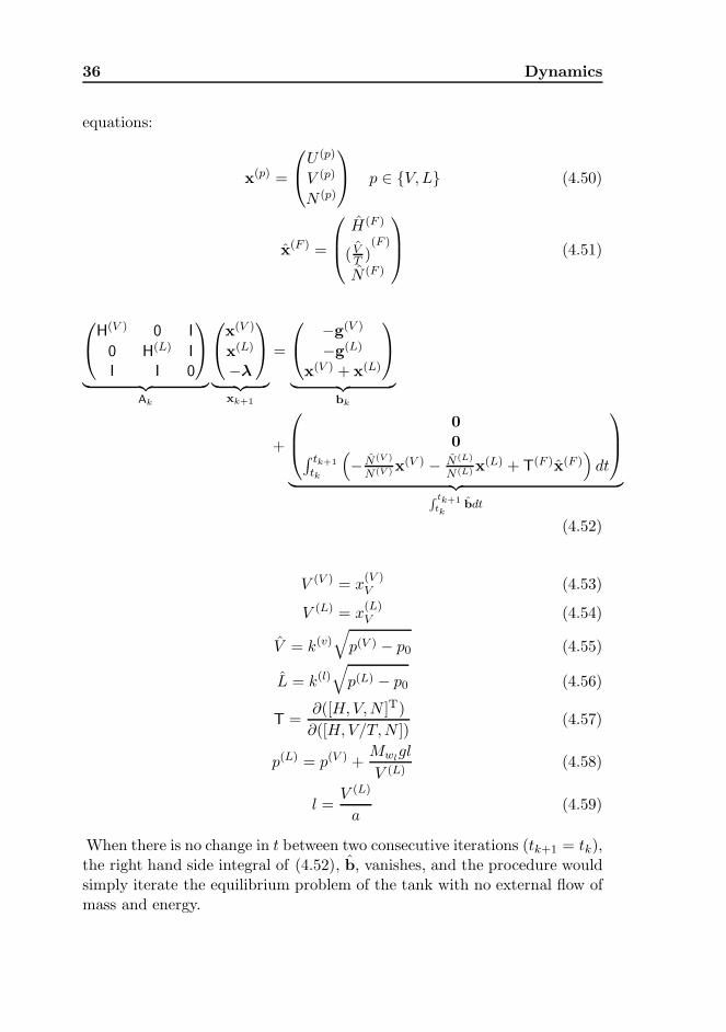
The minimization problem should be formulated in the most suitablevariables: the canonical variables – not necessarily T and p which is thetraditional choice. The conservation of internal energy and mass, with con-stant total volume of the separator suggest a minimization of −S(U, V,N)with flows in F (H, ˙(V/T ), N). To incorporate mass and energy transportover the time ∆t, an extra term is added on the right hand side of the
36 Dynamics
equations:
x(p) =
U (p)
V (p)
N (p)
p ∈ V,L (4.50)
x(F ) =
H(F )
ˆ(VT )
(F )
N (F )
(4.51)
H(V ) 0 I
0 H(L) I
I I 0
︸ ︷︷ ︸
Ak
x(V )
x(L)
−λ
︸ ︷︷ ︸
xk+1
=
−g(V )
−g(L)
x(V ) + x(L)
︸ ︷︷ ︸
bk
+
00
∫ tk+1
tk
(
− N(V )
N(V ) x(V ) − N(L)
N(L) x(L) + T(F )x(F )
)
dt
︸ ︷︷ ︸R tk+1
tkbdt
(4.52)
V (V ) = x(V )V (4.53)
V (L) = x(L)V (4.54)
V = k(v)√
p(V ) − p0 (4.55)
L = k(l)√
p(L) − p0 (4.56)
T =∂([H,V,N ]T)
∂([H,V/T,N ])(4.57)
p(L) = p(V ) +Mwl
gl
V (L)(4.58)
l =V (L)
a(4.59)
When there is no change in t between two consecutive iterations (tk+1 = tk),the right hand side integral of (4.52), b, vanishes, and the procedure wouldsimply iterate the equilibrium problem of the tank with no external flow ofmass and energy.
4.3. The dynamic Newton-Lagrange-Euler formulation 37
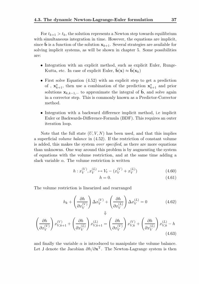
For tk+1 > tk, the solution represents a Newton step towards equilibriumwith simultaneous integration in time. However, the equations are implicit,since b is a function of the solution xk+1. Several strategies are available forsolving implicit systems, as will be shown in chapter 5. Some possibilitiesare:
• Integration with an explicit method, such as explicit Euler, Runge-Kutta, etc. In case of explicit Euler, b(x) ≈ b(xk)
• First solve Equation (4.52) with an explicit step to get a predictionof , x⋆
k+1, then use a combination of the prediction x⋆k+1 and prior
solutions xk,k−1,··· to approximate the integral of b, and solve againin a corrector step. This is commonly known as a Predictor-Correctormethod.
• Integration with a backward difference implicit method, i.e implicitEuler or Backwards-Difference-Formula (BDF). This requires an outeriteration loop.
Note that the full state (U, V,N) has been used, and that this impliesa superficial volume balance in (4.52). If the restriction of constant volumeis added, this makes the system over specified, as there are more equationsthan unknowns. One way around this problem is by augmenting the systemof equations with the volume restriction, and at the same time adding aslack variable α. The volume restriction is written
h : x(V )V , x
(L)V 7→ Vt − (x
(V )V + x
(L)V ) (4.60)
h = 0. (4.61)
The volume restriction is linearized and rearranged
hk +
(
∂h
∂x(V )V
)
∆x(V )V +
(
∂h
∂x(L)V
)
∆x(L)V = 0 (4.62)
⇓(
∂h
∂x(V )V
)
x(V )V,k+1 +
(
∂h
∂x(L)V
)
x(L)V,k+1 =
(
∂h
∂x(V )V
)
x(V )V,k +
(
∂h
∂x(L)V
)
x(L)V,k − h
(4.63)
and finally the variable α is introduced to manipulate the volume balance.Let J denote the Jacobian ∂h/∂xT. The Newton-Lagrange system is then
38 Dynamics
augmented with the volume restriction to
(Ak E
Jk 0
)(xk+1
α
)
=
(bk
Jkxk − h
)
+
(∫ t+∆tt bdt
0
)
(4.64)
where the matrix E is simply a selection matrix to let α adjust the balanceequation in volume.
4.4 Coupled minimization problems - dynamic case
In the previous section a set of equations was written for integrating a simpledynamic flash (4.64). In this section, the formulation for the connection ofseveral minimization problems will be shown.
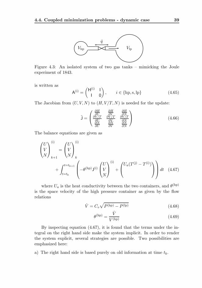
The celebrated Joule experiment [Joule, 1884] is used as an example.In his original paper On the Changes of Temperature produced by the Rar-efaction and Condensation of Air, Joule describes an experiment in whichhe immersed two copper containers in a water bath, one with dry air at 22atmospheres, the other close to vacuum. The two containers were separatedby a valve, and Joule was interested in the change of temperature in thewater bath when the stopcock was opened and the air expanded into theevacuated cylinder. A sketch of the experiment (excluding the water bathand thermometer) is shown in Figure 4.3. Joule recorded the temperature,and concluded that
The difference between the means of the expansions and alter-ations being exactly such as was found to be due to the increasedeffect of the temperature of the room in the latter case, we arriveat the conclusion, that no change of temperature occurs when airis allowed to expand in such a manner as not to develop mechan-ical power.1
This experiment can be modeled as two connected equilibrium problemsshowing an exchange of mass and energy. The tanks is modeled in variablesthat are explicitly used as constraint variables, thus the minimizations arein −S(U, V,N). The flow between the two tanks is conveniently representedby the set of canonical variables (H,V/T,N). Denoting the high pressurecylinder, the stream and the low pressure side with superscripts hp, s, lp, re-spectively, the coefficient matrix A for the individual minimization problems
1Later, Joule and Thompson found that for non-ideal gases there would be an temper-ature change under adiabatic expansion, known as the Joule-Thompson effect.
4.4. Coupled minimization problems - dynamic case 39
Vhp
q
Vlp
Figure 4.3: An isolated system of two gas tanks – mimicking the Jouleexperiment of 1843.
is written as
A(i) =
(H(i) I
I 0
)
, i ∈ hp, s, lp (4.65)
The Jacobian from (U, V,N) to (H,V/T,N) is needed for the update:
J =
∂H∂U
∂H∂V
∂H∂N
∂V/T∂U
∂V/T∂V
∂V/T∂N
∂N∂U
∂N∂V
∂N∂N
(4.66)
The balance equations are given as
UVN
(i)
k+1
=
UVN
(i)
k
+
∫ t=tk+1
t=tk
−θ(hp)J(i)
UVN
(i)
+
Ua(T(j) − T (i))
dt (4.67)
where Ua is the heat conductivity between the two containers, and θ(hp)
is the space velocity of the high pressure container as given by the flowrelations
V = Cv
√
P (hp) − P (lp) (4.68)
θ(hp) =V
V (hp)(4.69)
By inspecting equation (4.67), it is found that the terms under the in-tegral on the right hand side make the system implicit. In order to renderthe system explicit, several strategies are possible. Two possibilities areemphasized here:
a) The right hand side is based purely on old information at time tk.
40 Dynamics
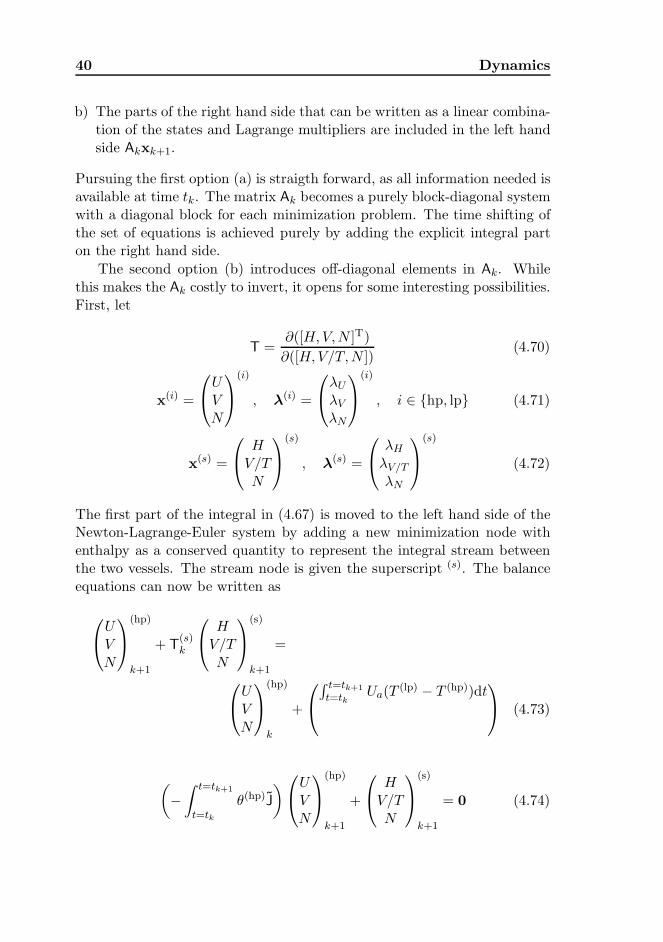
b) The parts of the right hand side that can be written as a linear combina-tion of the states and Lagrange multipliers are included in the left handside Akxk+1.
Pursuing the first option (a) is straigth forward, as all information needed isavailable at time tk. The matrix Ak becomes a purely block-diagonal systemwith a diagonal block for each minimization problem. The time shifting ofthe set of equations is achieved purely by adding the explicit integral parton the right hand side.
The second option (b) introduces off-diagonal elements in Ak. Whilethis makes the Ak costly to invert, it opens for some interesting possibilities.First, let
T =∂([H,V,N ]T)
∂([H,V/T,N ])(4.70)
x(i) =
UVN
(i)
, λ(i) =
λU
λV
λN
(i)
, i ∈ hp, lp (4.71)
x(s) =
HV/TN
(s)
, λ(s) =
λH
λV/T
λN
(s)
(4.72)
The first part of the integral in (4.67) is moved to the left hand side of theNewton-Lagrange-Euler system by adding a new minimization node withenthalpy as a conserved quantity to represent the integral stream betweenthe two vessels. The stream node is given the superscript (s). The balanceequations can now be written as
UVN
(hp)
k+1
+ T(s)k
HV/TN
(s)
k+1
=
UVN
(hp)
k
+
∫ t=tk+1
t=tkUa(T
(lp) − T (hp))dt
(4.73)
(
−∫ t=tk+1
t=tk
θ(hp)J
)
UVN
(hp)
k+1
+
HV/TN
(s)
k+1
= 0 (4.74)
4.4. Coupled minimization problems - dynamic case 41
T(s)k
HV/TN
(s)
k+1
+
UVN
(lp)
k+1
=
UVN
(lp)
k
+
∫ t=tk+1
t=tkUa(T
(hp) − T (lp))dt
(4.75)
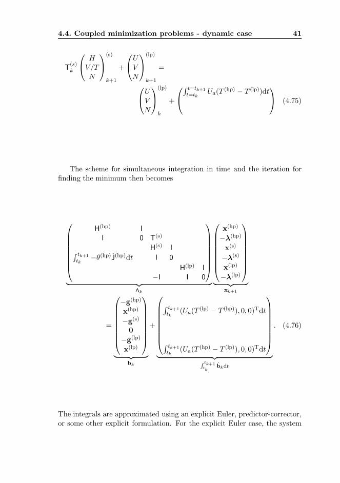
The scheme for simultaneous integration in time and the iteration forfinding the minimum then becomes
H(hp) I
I 0 T(s)
H(s) I∫ tk+1
tk−θ(hp)J(hp)dt I 0
H(lp) I
−I I 0
︸ ︷︷ ︸
Ak
x(hp)
−λ(hp)
x(s)
−λ(s)
x(lp)
−λ(lp)
︸ ︷︷ ︸
xk+1
=
−g(hp)
x(hp)
−g(s)
0
−g(lp)
x(lp)
︸ ︷︷ ︸
bk
+
∫ tk+1
tk(Ua(T
(lp) − T (hp)), 0, 0)Tdt
∫ tk+1
tk(Ua(T
(hp) − T (lp)), 0, 0)Tdt
︸ ︷︷ ︸R tk+1tk
bkdt
. (4.76)
The integrals are approximated using an explicit Euler, predictor-corrector,or some other explicit formulation. For the explicit Euler case, the system
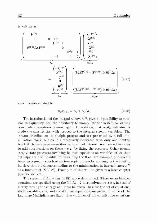
42 Dynamics
is written as
H(hp) I
I 0 T(s)
H(s) I
−θ(hp)∆tJ(hp) I 0
H(lp) I
−I I 0
︸ ︷︷ ︸
Ak
x(hp)
−λ(hp)
x(s)
−λ(s)
x(lp)
−λ(lp)
︸ ︷︷ ︸
xk+1
=
−g(hp)
x(hp)
−g(s)
0
−g(lp)
x(lp)
︸ ︷︷ ︸
bk
+
(Ua(T(lp) − T (hp)), 0, 0)T∆t
(Ua(T(hp) − T (lp)), 0, 0)T∆t
︸ ︷︷ ︸
bk∆t
(4.77)
which is abbreviated to
Akxk+1 = bk + bk∆t. (4.78)
The introduction of the integral stream x(s), gives the possibility to mon-itor this quantity, and the possibility to manipulate the system by writingconstitutive equations referencing it. In addition, matrix Ak will also in-clude the sensitivities with respect to the integral stream variables. Thestream describes an isenthalpic process and is represented by a full min-imization block, but could alternatively be stated with only one identityblock if the intensive quantities were not of interest, nor needed in orderto add specifications on those – e.g. by fixing the pressure. Other pseudosteady-state processes involving balance equations on variables other thanenthalpy are also possible for describing the flow. For example, the streambecomes a pseudo steady-state isentropic process by exchanging the identityblock with a block corresponding to the minimization in internal energy Uas a function of (S, V,N). Examples of this will be given in a later chapter(see Section 7.2).
The system of Equations (4.78) is overdetermined. Three extra balanceequations are specified using the full Nc+2 thermodynamic state, instead ofmerely stating the energy and mass balances. To close the set of equations,slack variables, α’s, and constitutive equations are given, or some of theLagrange-Multipliers are fixed. The variables of the constitutive equations
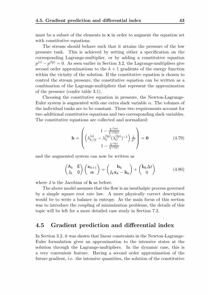
4.5. Gradient prediction and differential index 43
must be a subset of the elements in x in order to augment the equation setwith constitutive equations.
The stream should behave such that it attains the pressure of the lowpressure tank. This is achieved by setting either a specification on thecorresponding Lagrange-multiplier, or by adding a constitutive equationp(s)− p(lp) = 0. As seen earlier in Section 3.2, the Lagrange-multipliers givesecond order approximations to the k + 1 gradients of the energy functionwithin the vicinity of the solution. If the constitutive equation is chosen tocontrol the stream pressure, the constitutive equation can be written as acombination of the Lagrange-multipliers that represent the approximationof the pressure (confer table 3.1).
Choosing the constitutive equation in pressure, the Newton-Lagrange-Euler system is augmented with one extra slack variable α. The volumes ofthe individual tanks are to be constant. These two requirements account fortwo additional constitutive equations and two corresponding slack variables.The constitutive equations are collected and normalized:
h =
1− V (hp)
V (hp)(
λ(s)V/T − λ
(lp)V (λ
(lp)U )−1
)1p
1− V (lp)
V (lp)
= 0 (4.79)
and the augmented system can now be written as
(Ak E
Jk 0
)(xk+1
α
)
=
(bk
Jkxk − hk
)
+
(
bk∆t0
)
(4.80)
where J is the Jacobian of h as before.
The above model assumes that the flow is an isenthalpic process governedby a simple square root rate law. A more physically correct descriptionwould be to write a balance in entropy. As the main focus of this sectionwas to introduce the coupling of minimization problems, the details of thistopic will be left for a more detailed case study in Section 7.2.
4.5 Gradient prediction and differential index
In Section 3.2, it was shown that linear constraints in the Newton-Lagrange-Euler formulation gives an approximation to the intensive states at thesolution through the Lagrange-multipliers. In the dynamic case, this isa very convenient feature. Having a second order approximation of thefuture gradient, i.e. the intensive quantities, the solution of the constitutive
44 Dynamics
equations can be found at the end of each time step. Without this predictivecapability, one would have to resort to quadrature, using multiple steps.
As the careful reader might have noticed, the constitutive Equations(4.79) were stated in terms of the Lagrange multipliers, not in terms ofthe intensive quantities. As the predicted intensive quantities were used,and not the actual intensive quantities in the constitutive equations, theproblems of hidden constraints found in the usual DAE-formulation are notencountered. Thus it can be concluded that index problems do not occurin the dynamic Newton-Lagrange-Euler formulation.
Chapter 5
Simulating on canonical basis
Examples of how to formulate a model and how to define an iteration schemebased on canonical variables using the Newton-Lagrange-Euler formulationwere given in Chapter 4. This chapter will explain the methodology in moredetail and investigate some of its properties.
5.1 Building blocks
As examples in Section 4.4 showed, the coupled system of minimizationproblems, augmented with a linearization of constitutive equations can bewritten as
(Ak E
Jk 0
)(xk+1
α
)
=
(bk
Jkxk − hk
)
+
(bk∆t
0
)
(5.1)
The general diagonal building block is written
A(i,i) =
H(1) Q(1)T
H(2) Q(2)T
. . ....
H(ω) Q(ω)T
Q(1) Q(2) · · · Q(ω) 0
. (5.2)
5.1.1 The constraint matrix Q
The matrix Q(i) in Equation (5.2) is the product of a row-reduced transfor-mation from extensive quantities to conserved extensive quantities (energy,volume, atoms and inerts) Q, with a projection P(i) on the extensive quan-tities of phase (i) to a common minimal set of extensive quantities for all
45
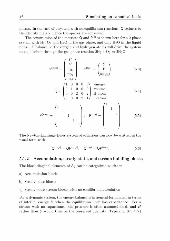
46 Simulating on canonical basis
phases. In the case of a system with no equilibrium reactions, Q reduces tothe identity matrix, hence the species are conserved.
The construction of the matrices Q and P(i) is shown here for a 2-phasesystem with H2, O2 and H2O in the gas phase, and only H2O in the liquidphase. A balance on the oxygen and hydrogen atoms will drive the systemto equilibrium through the gas phase reaction 2H2 + O2 2H2O.
x(vap) =
UV
nH2
nO2
nH2O
, x(liq) =
UV
nH2O
(5.3)
Q =
1 0 0 0 00 1 0 0 00 0 2 0 20 0 0 2 1
energyvolumeH-atomO-atom
(5.4)
P(vap) =
11
11
1
, P(liq) =
11
1
(5.5)
The Newton-Lagrange-Euler system of equations can now be written in theusual form with
Q(vap) = QP(vap), Q(liq) = QP(liq). (5.6)
5.1.2 Accumulation, steady-state, and stream building blocks
The block diagonal elements of Ak can be categorized as either
a) Accumulation blocks
b) Steady-state blocks
c) Steady-state stream blocks with no equilibrium calculation
For a dynamic system, the energy balance is in general formulated in termsof internal energy U when the equilibrium node has capacitance. For astream with no capacitance, the pressure is often assumed fixed, and Hrather than U would then be the conserved quantity. Typically, (U, V,N)
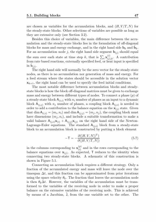
5.1. Building blocks 47
are chosen as variables for the accumulation blocks, and (H,V/T,N) forthe steady-state blocks. Other selections of variables are possible as long asthey are extensive only (see Section 3.2).
Besides this choice of variables, the main difference between the accu-mulation and the steady-state blocks lies in the formulation of off-diagonalblocks for mass and energy exchange, and in the right hand side bk and bk.For an accumulation node j, the right hand side segment b(j) should equal
the sum over each state at time step k, that is∑
i x(i)(j),k. A contribution
from rate based reactions, externally specified feed, or heat input is specifiedin b(j).
The right hand side will normally be the zero vector for the steady-statenodes, as there is no accumulation nor generation of mass and energy. Fora feed stream where the states should be accessible in the solution vectorxk+1, the right hand can be used to specify the feed initial conditions.
The most notable difference between accumulation blocks and steady-state blocks is how the block off-diagonal matrices must be given to exchangemass and energy between different types of nodes. To connect a phase (p) ofa steady-state block A(i,i) with ni number of phases as an input to a dynamicblock A(j,j) with nj number of phases, a coupling block A(j,i) is needed inorder to add a contribution to the balance equation on the x(j) state. Giventhat dim A(i,i) = (mi, ni) and dimA(j,j) = (mj , nj), the coupling block musthave dimensions (mj , ni), and include a suitable transformation to make avalid balance A(j,i)x(i) + A(j,j)x(j) on the right hand side of the Newton-Lagrange-Euler equations. The standard A(j,i) block from a steady-stateblock to an accumulation block is constructed by putting a block element
−T = − ∂([H,V,N ])T)
∂([H,V/T,N ])(5.7)
in the columns corresponding to x(p)(i) and in the rows corresponding to the
balance equations over x(j). As expected, T reduces to the identity whenconnecting two steady-state blocks. A schematic of this construction isshown in Figure 5.1.
Connecting an accumulation block requires a different strategy. Only afraction of the accumulated energy and mass will leave the node over thetimespan ∆t, and this fraction can be approximated from prior iterationsusing the space velocity θk. The fraction that leaves the accumulation nodeis then θk∆t. However, the variables of the accumulation must be trans-formed to the variables of the receiving node in order to make a properbalance on the extensive variables of the receiving node. This is achievedby means of a Jacobian, J, from the one variable set to the other. The
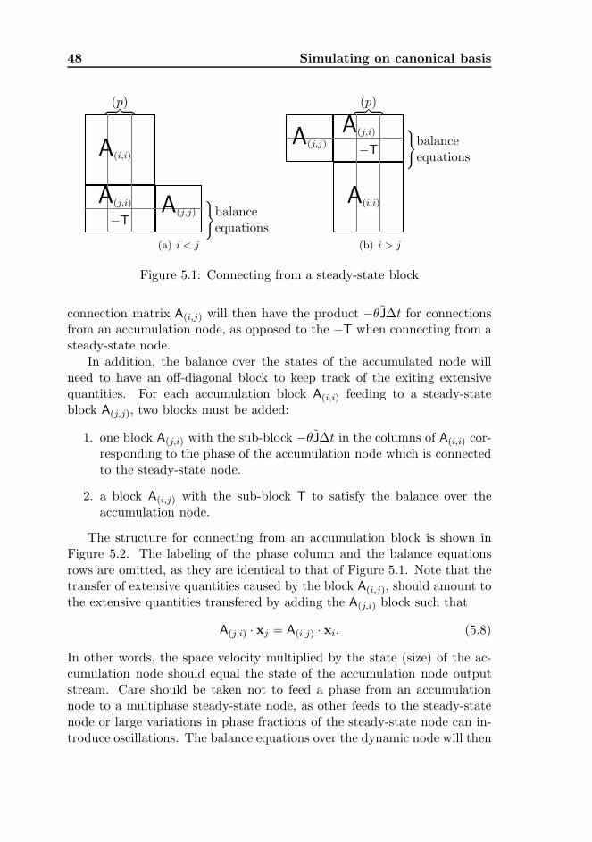
48 Simulating on canonical basis
A(j,i)
A(i,i)
A(j,j)−T
(p)
balanceequations
(a) i < j
A(j,j)
A(i,i)
A(j,i)
−T
(p)
balanceequations
(b) i > j
Figure 5.1: Connecting from a steady-state block
connection matrix A(i,j) will then have the product −θJ∆t for connectionsfrom an accumulation node, as opposed to the −T when connecting from asteady-state node.
In addition, the balance over the states of the accumulated node willneed to have an off-diagonal block to keep track of the exiting extensivequantities. For each accumulation block A(i,i) feeding to a steady-stateblock A(j,j), two blocks must be added:
1. one block A(j,i) with the sub-block −θJ∆t in the columns of A(i,i) cor-responding to the phase of the accumulation node which is connectedto the steady-state node.
2. a block A(i,j) with the sub-block T to satisfy the balance over theaccumulation node.
The structure for connecting from an accumulation block is shown inFigure 5.2. The labeling of the phase column and the balance equationsrows are omitted, as they are identical to that of Figure 5.1. Note that thetransfer of extensive quantities caused by the block A(i,j), should amount tothe extensive quantities transfered by adding the A(j,i) block such that
A(j,i) · xj = A(i,j) · xi. (5.8)
In other words, the space velocity multiplied by the state (size) of the ac-cumulation node should equal the state of the accumulation node outputstream. Care should be taken not to feed a phase from an accumulationnode to a multiphase steady-state node, as other feeds to the steady-statenode or large variations in phase fractions of the steady-state node can in-troduce oscillations. The balance equations over the dynamic node will then
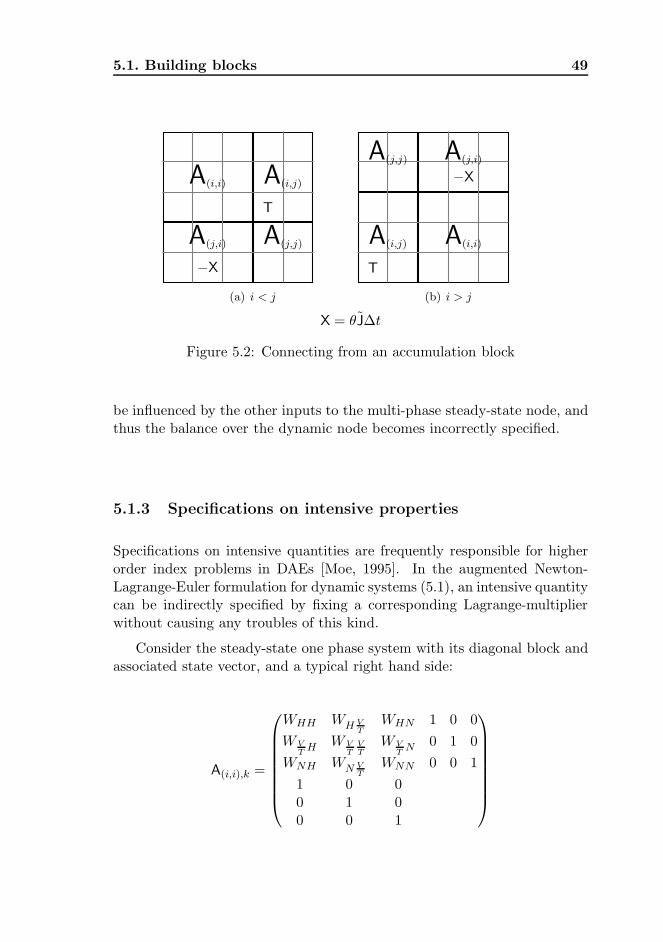
5.1. Building blocks 49
A(i,i) A(i,j)
A(j,i) A(j,j)
T
−X
(a) i < j
T
−X
A(j,j) A(j,i)
A(i,j) A(i,i)
(b) i > j
X = θJ∆t
Figure 5.2: Connecting from an accumulation block
be influenced by the other inputs to the multi-phase steady-state node, andthus the balance over the dynamic node becomes incorrectly specified.
5.1.3 Specifications on intensive properties
Specifications on intensive quantities are frequently responsible for higherorder index problems in DAEs [Moe, 1995]. In the augmented Newton-Lagrange-Euler formulation for dynamic systems (5.1), an intensive quantitycan be indirectly specified by fixing a corresponding Lagrange-multiplierwithout causing any troubles of this kind.
Consider the steady-state one phase system with its diagonal block andassociated state vector, and a typical right hand side:
A(i,i),k =
WHH WH VT
WHN 1 0 0
WVT
H WVT
VT
WVT
N 0 1 0
WNH WN VT
WNN 0 0 1
1 0 00 1 00 0 1
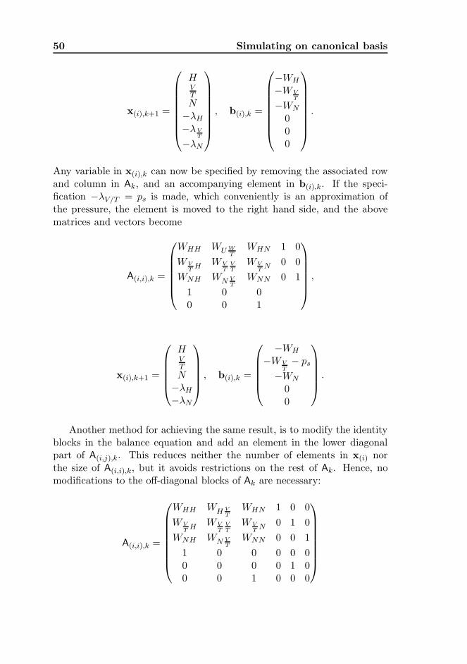
50 Simulating on canonical basis
x(i),k+1 =
HVTN−λH
−λVT
−λN
, b(i),k =
−WH
−WVT
−WN
000
.
Any variable in x(i),k can now be specified by removing the associated rowand column in Ak, and an accompanying element in b(i),k. If the speci-fication −λV/T = ps is made, which conveniently is an approximation ofthe pressure, the element is moved to the right hand side, and the abovematrices and vectors become
A(i,i),k =
WHH WU WT
WHN 1 0
WVT
H WVT
VT
WVT
N 0 0
WNH WN VT
WNN 0 1
1 0 00 0 1
,
x(i),k+1 =
HVTN−λH
−λN
, b(i),k =
−WH
−WVT− ps
−WN
00
.
Another method for achieving the same result, is to modify the identityblocks in the balance equation and add an element in the lower diagonalpart of A(i,j),k. This reduces neither the number of elements in x(i) northe size of A(i,i),k, but it avoids restrictions on the rest of Ak. Hence, nomodifications to the off-diagonal blocks of Ak are necessary:
A(i,i),k =
WHH WH VT
WHN 1 0 0
WVT
H WVT
VT
WVT
N 0 1 0
WNH WN VT
WNN 0 0 1
1 0 0 0 0 00 0 0 0 1 00 0 1 0 0 0
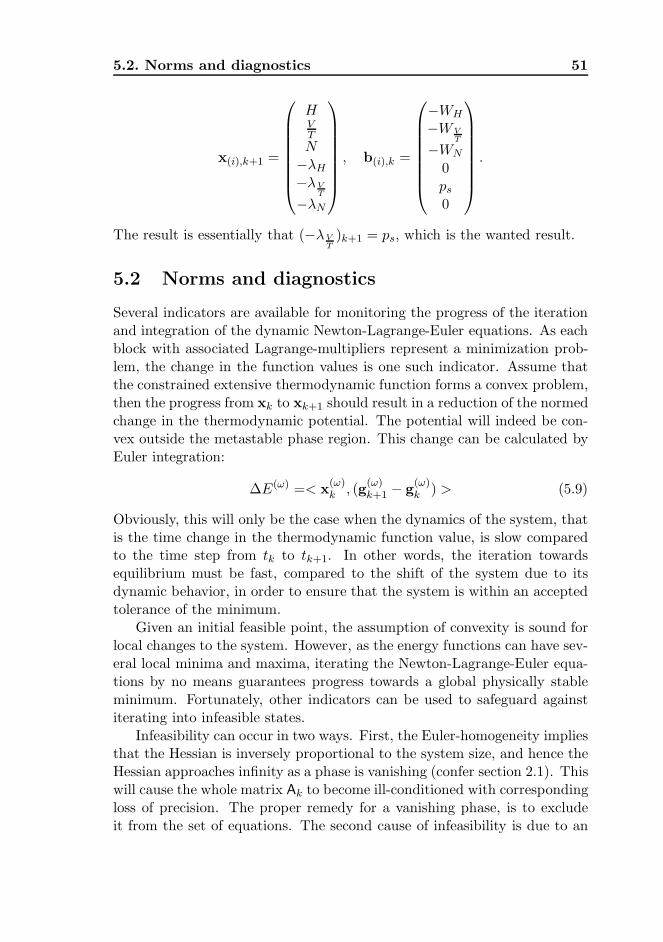
5.2. Norms and diagnostics 51
x(i),k+1 =
HVTN−λH
−λVT
−λN
, b(i),k =
−WH
−WVT
−WN
0ps
0
.
The result is essentially that (−λVT
)k+1 = ps, which is the wanted result.
5.2 Norms and diagnostics
Several indicators are available for monitoring the progress of the iterationand integration of the dynamic Newton-Lagrange-Euler equations. As eachblock with associated Lagrange-multipliers represent a minimization prob-lem, the change in the function values is one such indicator. Assume thatthe constrained extensive thermodynamic function forms a convex problem,then the progress from xk to xk+1 should result in a reduction of the normedchange in the thermodynamic potential. The potential will indeed be con-vex outside the metastable phase region. This change can be calculated byEuler integration:
∆E(ω) =< x(ω)k , (g
(ω)k+1 − g
(ω)k ) > (5.9)
Obviously, this will only be the case when the dynamics of the system, thatis the time change in the thermodynamic function value, is slow comparedto the time step from tk to tk+1. In other words, the iteration towardsequilibrium must be fast, compared to the shift of the system due to itsdynamic behavior, in order to ensure that the system is within an acceptedtolerance of the minimum.
Given an initial feasible point, the assumption of convexity is sound forlocal changes to the system. However, as the energy functions can have sev-eral local minima and maxima, iterating the Newton-Lagrange-Euler equa-tions by no means guarantees progress towards a global physically stableminimum. Fortunately, other indicators can be used to safeguard againstiterating into infeasible states.
Infeasibility can occur in two ways. First, the Euler-homogeneity impliesthat the Hessian is inversely proportional to the system size, and hence theHessian approaches infinity as a phase is vanishing (confer section 2.1). Thiswill cause the whole matrix Ak to become ill-conditioned with correspondingloss of precision. The proper remedy for a vanishing phase, is to excludeit from the set of equations. The second cause of infeasibility is due to an
52 Simulating on canonical basis
instable or a metastable phase. For a minimization of a thermodynamicpotential, e.g. min(−S) or min U , a positive semidefinite Hessian impliesa stable phase. Conversely, an indefinite Hessian implies an intrinsic phaseinstability. However, if the inclusion of a new trial phase does lower theobjective function further, the current topology is metastable and a newtrial phase must be included in the block. Stability testing is not a topic ofthis work, and the metastable case has not been considered, although this isclearly important for the general applicability of the described methods. Thereader is referred to Haug-Warberg [1988], Brendsdal [1999] and Michelsen[1982] for a detailed analysis.
Another useful indicator stems from the Lagrange-multipliers. As wasshown in section 3.2, the Lagrange-multipliers give second order approxi-mations to the gradient of the thermodynamic potentials in vicinity of thesolution. Monitoring the discrepancy between the prediction λk+1 from thesolution vector xk+1, and the calculated gradient gk+1 (after updating thestate), therefore gives an indication of how well the Lagrange-multiplierspredict the future intensive quantities. If the prediction is off by more thana given tolerance, the system is either becoming ill-conditioned, or the timeresolution is not fine enough to follow an induced dynamic transient.
The last indicator suggested here is the change in the space velocity ofan accumulation node phase θ. The value of θ represents the fraction ofa given phase in an accumulation node that exits the node per unit time.If the integral of
∫ tk+1
tkθdt approaches unity, the flow through this phase
becomes as large as the contents of the phase itself. This implies that thecomplete contents of the phase at time tk is emptied from tk to tk+1, andreplaced by whatever enters the node. If this is the case for an arbitrarytime interval, the node is more appropriately described as being in a pseudosteady-state condition, saying that whatever enters over the time interval,will exit and not accumulate. Conversely, if the integral approaches unityduring the course of the iteration, this is an indication of the dynamicsof the node being too fast to be accurately described by the current timeresolution (the integration horizon for θ).
To summarize, the following indicators can be monitored:
a) The progress of the combined iteration-integration by tracking the changein the extensive thermodynamic function of each phase
b) The discrepancy between the prediction of future intensive quantities(λk+1) to the actual updated intensive quantities (gk+1)
c) The magnitude of the space velocities (θ) compared to the time step.
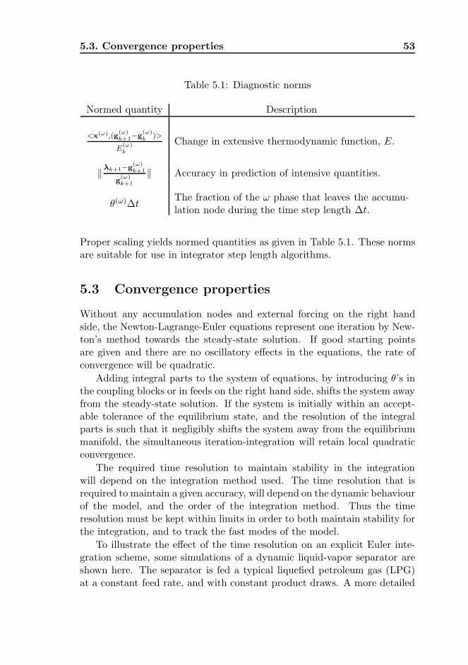
5.3. Convergence properties 53
Table 5.1: Diagnostic norms
Normed quantity Description
<x(ω),(g(ω)k+1−g
(ω)k
)>
E(ω)k
Change in extensive thermodynamic function, E.
‖λk+1−g(ω)k+1
g(ω)k+1
‖ Accuracy in prediction of intensive quantities.
θ(ω)∆tThe fraction of the ω phase that leaves the accumu-lation node during the time step length ∆t.
Proper scaling yields normed quantities as given in Table 5.1. These normsare suitable for use in integrator step length algorithms.
5.3 Convergence properties
Without any accumulation nodes and external forcing on the right handside, the Newton-Lagrange-Euler equations represent one iteration by New-ton’s method towards the steady-state solution. If good starting pointsare given and there are no oscillatory effects in the equations, the rate ofconvergence will be quadratic.
Adding integral parts to the system of equations, by introducing θ’s inthe coupling blocks or in feeds on the right hand side, shifts the system awayfrom the steady-state solution. If the system is initially within an accept-able tolerance of the equilibrium state, and the resolution of the integralparts is such that it negligibly shifts the system away from the equilibriummanifold, the simultaneous iteration-integration will retain local quadraticconvergence.
The required time resolution to maintain stability in the integrationwill depend on the integration method used. The time resolution that isrequired to maintain a given accuracy, will depend on the dynamic behaviourof the model, and the order of the integration method. Thus the timeresolution must be kept within limits in order to both maintain stability forthe integration, and to track the fast modes of the model.
To illustrate the effect of the time resolution on an explicit Euler inte-gration scheme, some simulations of a dynamic liquid-vapor separator areshown here. The separator is fed a typical liquefied petroleum gas (LPG)at a constant feed rate, and with constant product draws. A more detailed
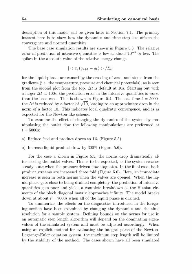
54 Simulating on canonical basis
description of this model will be given later in Section 7.1. The primaryinterest here is to show how the dynamics and time step size affects theconvergence and normed quantities.
The base case simulation results are shown in Figure 5.3. The relativeerror in prediction of intensive quantities is low at about 10−5 or less. Thespikes in the absolute value of the relative energy change
| < x, (gk+1 − gk) > /Ek|
for the liquid phase, are caused by the crossing of zero, and stems from thegradients (i.e. the temperature, pressure and chemical potentials), as is seenfrom the second plot from the top. ∆t is default at 10s. Starting out witha larger ∆t at 100s, the prediction error in the intensive quantities is worsethan the base case. This is shown in Figure 5.4. Then at time t = 5000sthe ∆t is reduced by a factor of
√10, leading to an approximate drop in the
norm of a factor 10. This indicates local quadratic convergence, and is asexpected for the Newton-like scheme.
To examine the effect of changing the dynamics of the system by ma-nipulating the outlet flow the following manipulations are preformed att = 5000s:
a) Reduce feed and product draws to 1% (Figure 5.5).
b) Increase liquid product draw by 300% (Figure 5.6).
For the case a shown in Figure 5.5, the norms drop dramatically af-ter closing the outlet valves. This is to be expected, as the system reachessteady state when the pressure driven flow stagnates. In the final case, bothproduct streams are increased three fold (Figure 5.6). Here, an immediateincrease is seen in both norms when the valves are opened. When the liq-uid phase gets close to being drained completely, the prediction of intensivequantities gets poor and yields a complete breakdown as the Hessian ele-ments of the block diagonal matrix approaches infinity. The model breaksdown at about t = 7000s when all of the liquid phase is drained.
To summarize, the effects on the diagnostics introduced in the forego-ing section have been examined by changing the dynamics and the timeresolution for a sample system. Defining bounds on the norms for use inan automatic step length algorithm will depend on the dominating eigen-values of the simulated system and must be adjusted accordingly. Whenusing an explicit method for evaluating the integral parts of the Newton-Lagrange-Euler equation system, the maximum step length will be limitedby the stability of the method. The cases shown have all been simulated
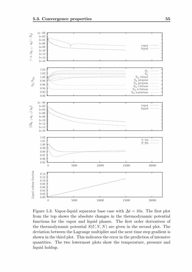
5.3. Convergence properties 55
1e-16 1e-14 1e-12 1e-10 1e-08 1e-06 1e-04 1e-02
1e+00|<
x, (
g k+
1 -
g k)>
/Ek|
vaporliquid
0.90 0.92 0.94 0.96 0.98 1.00 1.02 1.04
SX/S
X0
SUSV
SN ethaneSN propeneSN propaneSN i-butaneSN n-butane
SN n-pentane
1e-16 1e-14 1e-12 1e-10 1e-08 1e-06 1e-04 1e-02
1e+00
||(λ
k+1-
g k+
1)/g
k|| vapor
liquid
0.95 0.96 0.97 0.98 0.99 1.00 1.01 1.02
0 5000 10000 15000 20000
T/T0P/P0
0.00 0.02 0.04 0.06 0.08 0.10 0.12 0.14
0 5000 10000 15000 20000
Liq
ud v
olum
e fr
acti
on
Figure 5.3: Vapor-liquid separator base case with ∆t = 10s. The first plotfrom the top shows the absolute changes in the thermodynamic potentialfunctions for the vapor and liquid phases. The first order derivatives ofthe thermodynamic potential S(U, V,N) are given in the second plot. Thedeviation between the Lagrange multiplier and the next time step gradient isshown in the third plot. This indicates the error in the prediction of intensivequantities. The two lowermost plots show the temperature, pressure andliquid holdup.
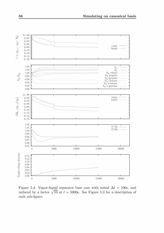
56 Simulating on canonical basis
1e-16 1e-14 1e-12 1e-10 1e-08 1e-06 1e-04 1e-02
1e+00
|<x,
(g k
+1
- g k
)>/E
k|
vaporliquid
0.90 0.92 0.94 0.96 0.98 1.00 1.02 1.04
SX/S
X0
SUSV
SN ethaneSN propeneSN propaneSN i-butaneSN n-butane
SN n-pentane
1e-16 1e-14 1e-12 1e-10 1e-08 1e-06 1e-04 1e-02
1e+00
||(λ
k+1-
g k+
1)/g
k|| vapor
liquid
0.95 0.96 0.97 0.98 0.99 1.00 1.01 1.02
0 5000 10000 15000 20000
T/T0P/P0
0.00 0.02 0.04 0.06 0.08 0.10 0.12 0.14
0 5000 10000 15000 20000
Liq
ud v
olum
e fr
action
Figure 5.4: Vapor-liquid separator base case with initial ∆t = 100s, andreduced by a factor
√10 at t = 5000s. See Figure 5.3 for a description of
each sub-figure.
5.3. Convergence properties 57
1e-16 1e-14 1e-12 1e-10 1e-08 1e-06 1e-04 1e-02
1e+00
|<x,
(g k
+1
- g k
)>/E
k|
vaporliquid
0.90 0.92 0.94 0.96 0.98 1.00 1.02 1.04
SX/S
X0
SUSV
SN ethaneSN propeneSN propaneSN i-butaneSN n-butane
SN n-pentane
1e-16 1e-14 1e-12 1e-10 1e-08 1e-06 1e-04 1e-02
1e+00
||(λ
k+1-
g k+
1)/g
k|| vapor
liquid
0.95 0.96 0.97 0.98 0.99 1.00 1.01 1.02
0 5000 10000 15000 20000
T/T0P/P0
0.00 0.02 0.04 0.06 0.08 0.10 0.12 0.14
0 5000 10000 15000 20000
Liq
ud v
olum
e fr
action
Figure 5.5: Vapor-liquid separator, with feed and product streams set to1% at time t = 5000s. See Figure 5.3 for a description of each sub-figure.
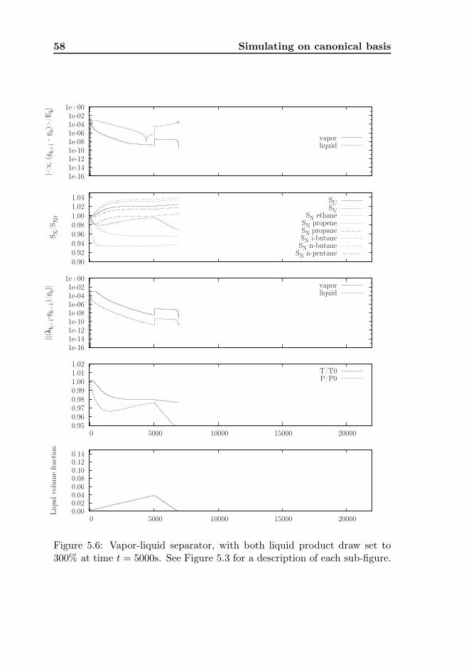
58 Simulating on canonical basis
1e-16 1e-14 1e-12 1e-10 1e-08 1e-06 1e-04 1e-02
1e+00
|<x,
(g k
+1
- g k
)>/E
k|
vaporliquid
0.90 0.92 0.94 0.96 0.98 1.00 1.02 1.04
SX/S
X0
SUSV
SN ethaneSN propeneSN propaneSN i-butaneSN n-butane
SN n-pentane
1e-16 1e-14 1e-12 1e-10 1e-08 1e-06 1e-04 1e-02
1e+00
||(λ
k+1-
g k+
1)/g
k|| vapor
liquid
0.95 0.96 0.97 0.98 0.99 1.00 1.01 1.02
0 5000 10000 15000 20000
T/T0P/P0
0.00 0.02 0.04 0.06 0.08 0.10 0.12 0.14
0 5000 10000 15000 20000
Liq
ud v
olum
e fr
action
Figure 5.6: Vapor-liquid separator, with both liquid product draw set to300% at time t = 5000s. See Figure 5.3 for a description of each sub-figure.
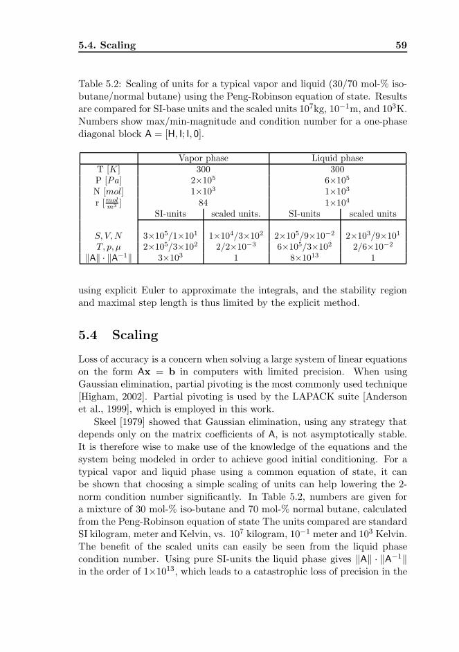
5.4. Scaling 59
Table 5.2: Scaling of units for a typical vapor and liquid (30/70 mol-% iso-butane/normal butane) using the Peng-Robinson equation of state. Resultsare compared for SI-base units and the scaled units 107kg, 10−1m, and 103K.Numbers show max/min-magnitude and condition number for a one-phasediagonal block A = [H, I; I, 0].
Vapor phase Liquid phaseT [K] 300 300P [Pa] 2×10⁵ 6×10⁵
N [mol] 1×10³ 1×10³
r [mol
m3 ] 84 1×10⁴
SI-units scaled units. SI-units scaled units
S, V, N 3×10⁵/1×101 1×10⁴/3×102 2×10⁵/9×10−2 2×10³/9×101
T, p, µ 2×10⁵/3×102 2/2×10−3 6×10⁵/3×102 2/6×10−2
‖A‖ · ‖A−1‖ 3×10³ 1 8×10¹³ 1
using explicit Euler to approximate the integrals, and the stability regionand maximal step length is thus limited by the explicit method.
5.4 Scaling
Loss of accuracy is a concern when solving a large system of linear equationson the form Ax = b in computers with limited precision. When usingGaussian elimination, partial pivoting is the most commonly used technique[Higham, 2002]. Partial pivoting is used by the LAPACK suite [Andersonet al., 1999], which is employed in this work.
Skeel [1979] showed that Gaussian elimination, using any strategy thatdepends only on the matrix coefficients of A, is not asymptotically stable.It is therefore wise to make use of the knowledge of the equations and thesystem being modeled in order to achieve good initial conditioning. For atypical vapor and liquid phase using a common equation of state, it canbe shown that choosing a simple scaling of units can help lowering the 2-norm condition number significantly. In Table 5.2, numbers are given fora mixture of 30 mol-% iso-butane and 70 mol-% normal butane, calculatedfrom the Peng-Robinson equation of state The units compared are standardSI kilogram, meter and Kelvin, vs. 107 kilogram, 10−1 meter and 103 Kelvin.The benefit of the scaled units can easily be seen from the liquid phasecondition number. Using pure SI-units the liquid phase gives ‖A‖ · ‖A−1‖in the order of 1×10¹³, which leads to a catastrophic loss of precision in the
60 Simulating on canonical basis
Gaussian elimination. Starting out with double precision and a mantissaof 53 bits, the initial number of significant digits are 15. After Gaussianelimination and back substitution, there are only two significant digits left.
The above example shows how a simple scaling of the scientific units canovercome, at least partially, the degeneration of the solution without havingto rewrite the model equations. The scaling shown with 107kg, 10−1m, and103K, and SI-base units otherwise is used for all internal calculation in thiswork. No modification or normalization of the equations are preformed toincrease the precision further.
Chapter 6
The dynamic
Newton-Lagrange-Euler
simulator
The effort required to in updating the structures used by the numericalscheme can be substantial for a model of some complexity. Simulationwith the dynamic Newton-Lagrange-Euler formulation requires for everyiteration step k the evaluation of:
a) Explicit thermodynamic functions with derivatives.
b) Legendre transform and Massieu function with derivatives.
c) Jacobian from one canonical variable set to another, and from the trans-formed coordinates to the explicit variables of the thermodynamic sur-face.
d) The right hand side elements bk and bk∆t.
e) Diagonal sub blocks and connection blocks.
f) Constitutive equations h with derivatives.
All this is needed in order to solve Equation (5.1) for xk+1, and to updatethe thermodynamic function variables via Jacobians. Needless to say, thereis a lot of bookkeeping involved for larger systems.
Inspired by the steady-state simulator Yasim[Siepmann, 2006], a proto-type of a tool for automating the equation system construction and evalu-ation was developed. The acronym DYNLE - DYnamic Newton-Lagrange-
61
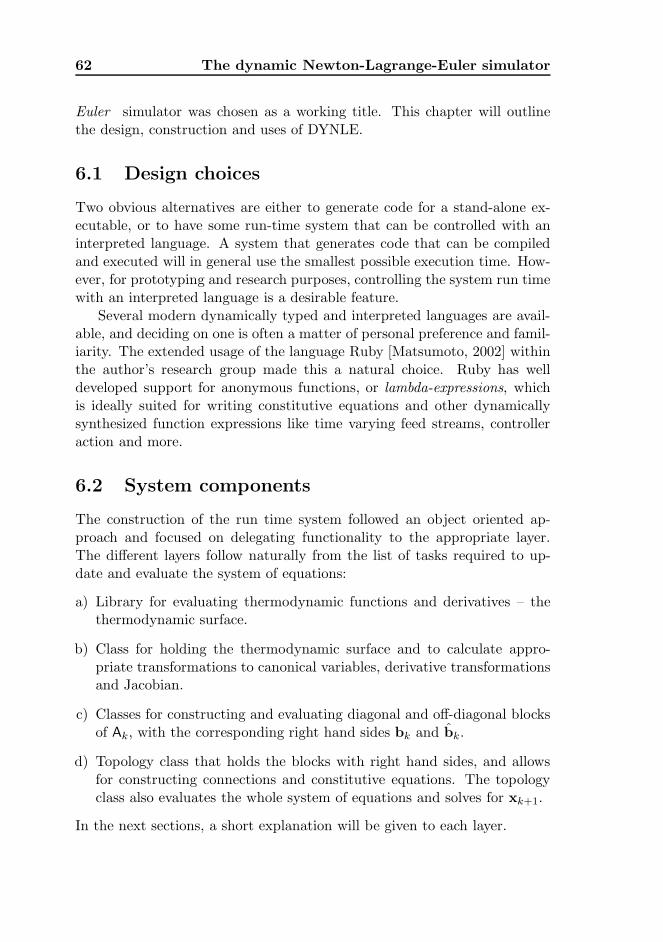
62 The dynamic Newton-Lagrange-Euler simulator
Euler simulator was chosen as a working title. This chapter will outlinethe design, construction and uses of DYNLE.
6.1 Design choices
Two obvious alternatives are either to generate code for a stand-alone ex-ecutable, or to have some run-time system that can be controlled with aninterpreted language. A system that generates code that can be compiledand executed will in general use the smallest possible execution time. How-ever, for prototyping and research purposes, controlling the system run timewith an interpreted language is a desirable feature.
Several modern dynamically typed and interpreted languages are avail-able, and deciding on one is often a matter of personal preference and famil-iarity. The extended usage of the language Ruby [Matsumoto, 2002] withinthe author’s research group made this a natural choice. Ruby has welldeveloped support for anonymous functions, or lambda-expressions, whichis ideally suited for writing constitutive equations and other dynamicallysynthesized function expressions like time varying feed streams, controlleraction and more.
6.2 System components
The construction of the run time system followed an object oriented ap-proach and focused on delegating functionality to the appropriate layer.The different layers follow naturally from the list of tasks required to up-date and evaluate the system of equations:
a) Library for evaluating thermodynamic functions and derivatives – thethermodynamic surface.
b) Class for holding the thermodynamic surface and to calculate appro-priate transformations to canonical variables, derivative transformationsand Jacobian.
c) Classes for constructing and evaluating diagonal and off-diagonal blocksof Ak, with the corresponding right hand sides bk and bk.
d) Topology class that holds the blocks with right hand sides, and allowsfor constructing connections and constitutive equations. The topologyclass also evaluates the whole system of equations and solves for xk+1.
In the next sections, a short explanation will be given to each layer.
6.2. System components 63
6.2.1 Thermodynamic functions and analytical derivatives
Haug-Warberg [2003] has developed a systematic algebra for synthesizingthermodynamic energy functions, and a tool chain to generate function ex-pressions and serialize the function representation. This algebra and toolsmakes it possible to generate consistent functions with all required param-eters, standard states, mixing rules, heat capacity expressions, etc. Furtherwork resulted in the RGrad-system by Løvfall [2008] which uses this serial-ization to generate arbitrary order function gradients, and generates code forthe function and gradient evaluation in the C-language, including wrappersfor the Ruby, Matlab and Octave interpreters. Using these tools resultsin enormous time savings in the implementation, compared to collectingparameters and writing function and function derivatives by hand.
6.2.2 Manifolds of Legendre transforms and Massieu func-
tions
The sets of Legendre transforms and Massieu functions required to map thevariables of the surface to the coordinates of the pertinent thermodynamicmanifold in canonical variables are dictated by the thermodynamic surface,and can thus be deduced automatically. The manifold needs to be initial-ized, either by assigning initial values to the surface variables, or by iterationat given manifold coordinates. Given updates in the manifold coordinates,the Jacobian can be applied to linearly approximate the update of surfacevariables.
The structure of the thermodynamic surface and some rough checks candetermine whether the proposed update of surface variables is feasible. Thechecks can include testing for the logarithm of a negative number, divisionby zero, asserting that the volume is greater than the hard sphere volume(Vm > b in the cubic equations of state), asserting the values are withinthe valid range for extrapolation, etc. This checking is a feature of theThermo/RGrad system, and it allows the possibility of testing differentupdate step lengths.
A handy feature of the manifold-implementation in DYNLE is to knowwhich surface variables are intensive, and which are extensive, thereby mak-ing it possible to scale the system by a simple method call.
6.2.3 Blocks and right hand sides
A diagonal block can be created by deciding the set of canonical variablesand whether the block represents a node that can accumulate the extensive
64 The dynamic Newton-Lagrange-Euler simulator
quantities. Typically, an accumulation block is created by assigning thecanonical variables (U, V,N) variables. A steady-state block will in generaluse the (H,V/T,N) variables. A thermodynamic surface is assigned to eachphase of the node at creation. For each block type, there is an associateddefault right hand side. The default can be overridden by supplying alambda-expression that evaluates the right hand side. The block can bemodified to facilitate a specification on the relevant Lagrange multiplierand change the right hand side accordingly, given a specification on one ofthe intensive quantities,
When all the diagonal blocks are placed, connections can be made bycreating the off-diagonal coupling blocks. Once the originating block andphases are decided, the only required specification is which block will serveas the target. When the source is a phase of an accumulation node, alambda-expression that can be evaluated to find θ should be supplied.
6.2.4 Topology of blocks and connections
On the upper layer, an object is needed to hold all the blocks and the con-stitutive equations. This object is the topology. Having initialized a setof diagonal blocks, these are placed on the topology, and later connected.Each of the diagonal blocks have an associated degree of freedom from theextraneous balance equation. This degree of freedom stems from writingthe balance on the full set of Nc + 2 canonical variables. Only Nc + 1of these variables are tied to the mass and energy balance, and the sys-tem of equations can only be closed by either specifying the correspondingLagrange-multiplier, or by adding a constitutive equation for the last bal-ance equation.
When the construction of the topology is complete, everything needed toconstruct the system of equations (5.1) can be evaluated. By keeping trackof the norms described in Section 5.2, the step length ∆t can be manipulatedto keep the norms within desired bounds.
6.2.5 Linear algebra
Solving the linear equation system (5.1) at each iteration can be preformedwith most linear algebra packages. The LAPACK suite is a well establishedand extensively used set of subroutines specifically designed to handle largeequation systems [Anderson et al., 1999]. The main interfaces for these areavailable in the Fortran language. These subroutines rely on underlying sub-routines to handle scalar, vector and matrix operations that comply with
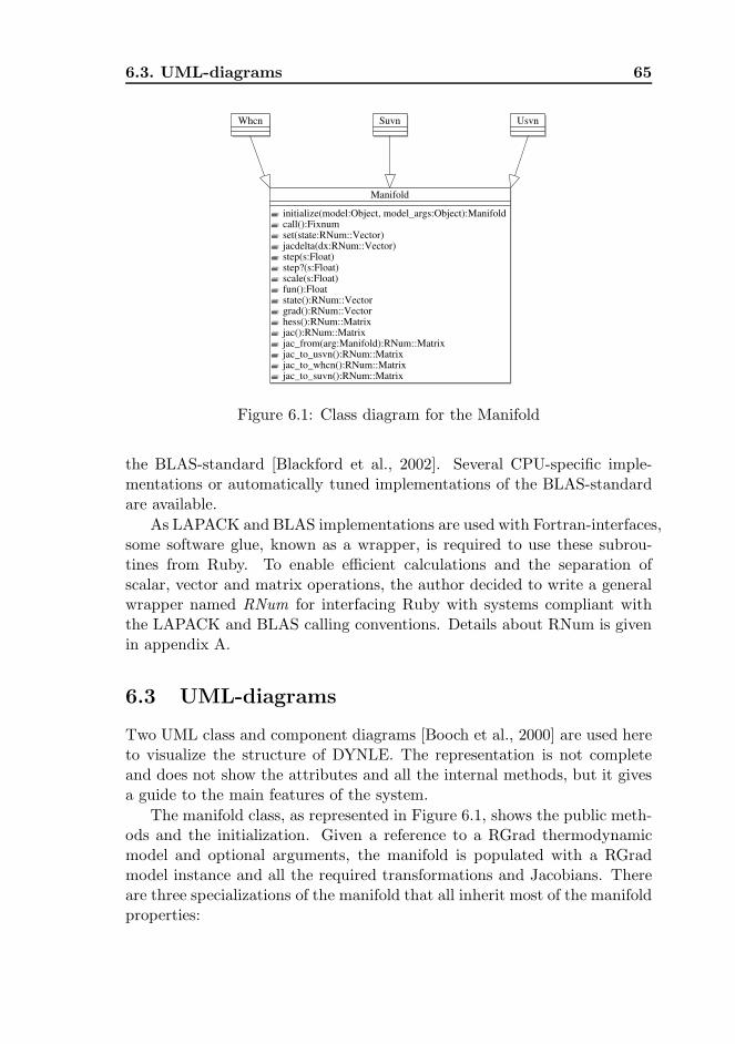
6.3. UML-diagrams 65
Manifold
initialize(model:Object, model_args:Object):Manifoldcall():Fixnumset(state:RNum::Vector)jacdelta(dx:RNum::Vector)step(s:Float)step?(s:Float)scale(s:Float)fun():Floatstate():RNum::Vectorgrad():RNum::Vectorhess():RNum::Matrixjac():RNum::Matrixjac_from(arg:Manifold):RNum::Matrixjac_to_usvn():RNum::Matrixjac_to_whcn():RNum::Matrixjac_to_suvn():RNum::Matrix
Whcn Suvn Usvn
Figure 6.1: Class diagram for the Manifold
the BLAS-standard [Blackford et al., 2002]. Several CPU-specific imple-mentations or automatically tuned implementations of the BLAS-standardare available.
As LAPACK and BLAS implementations are used with Fortran-interfaces,some software glue, known as a wrapper, is required to use these subrou-tines from Ruby. To enable efficient calculations and the separation ofscalar, vector and matrix operations, the author decided to write a generalwrapper named RNum for interfacing Ruby with systems compliant withthe LAPACK and BLAS calling conventions. Details about RNum is givenin appendix A.
6.3 UML-diagrams
Two UML class and component diagrams [Booch et al., 2000] are used hereto visualize the structure of DYNLE. The representation is not completeand does not show the attributes and all the internal methods, but it givesa guide to the main features of the system.
The manifold class, as represented in Figure 6.1, shows the public meth-ods and the initialization. Given a reference to a RGrad thermodynamicmodel and optional arguments, the manifold is populated with a RGradmodel instance and all the required transformations and Jacobians. Thereare three specializations of the manifold that all inherit most of the manifoldproperties:
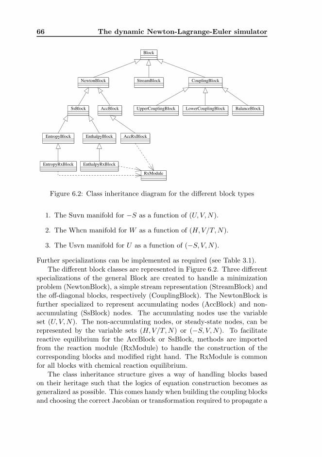
66 The dynamic Newton-Lagrange-Euler simulator
Block
StreamBlockNewtonBlock CouplingBlock
SsBlock AccBlock UpperCouplingBlock LowerCouplingBlock BalanceBlock
EntropyBlock EnthalpyBlock AccRxBlock
EntropyRxBlock EnthalpyRxBlock
RxModule
Figure 6.2: Class inheritance diagram for the different block types
1. The Suvn manifold for −S as a function of (U, V,N).
2. The Whcn manifold for W as a function of (H,V/T,N).
3. The Usvn manifold for U as a function of (−S, V,N).
Further specializations can be implemented as required (see Table 3.1).
The different block classes are represented in Figure 6.2. Three differentspecializations of the general Block are created to handle a minimizationproblem (NewtonBlock), a simple stream representation (StreamBlock) andthe off-diagonal blocks, respectively (CouplingBlock). The NewtonBlock isfurther specialized to represent accumulating nodes (AccBlock) and non-accumulating (SsBlock) nodes. The accumulating nodes use the variableset (U, V,N). The non-accumulating nodes, or steady-state nodes, can berepresented by the variable sets (H,V/T,N) or (−S, V,N). To facilitatereactive equilibrium for the AccBlock or SsBlock, methods are importedfrom the reaction module (RxModule) to handle the construction of thecorresponding blocks and modified right hand. The RxModule is commonfor all blocks with chemical reaction equilibrium.
The class inheritance structure gives a way of handling blocks basedon their heritage such that the logics of equation construction becomes asgeneralized as possible. This comes handy when building the coupling blocksand choosing the correct Jacobian or transformation required to propagate a
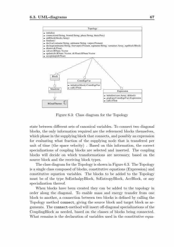
6.3. UML-diagrams 67
Topology
initializeconnect(toid:String, fromid:String, phase:String, theta:Proc)addblock(blocks:Array)finalize()declvar(varname:String, unitname:String, varpos:Fixnum)decleqn(unitname:String, freevarpos:Fixnum, eqnname:String, varnames:Array, eqnblock:Block)dtinit=(dt:Float)solve():RNum::Vectorupdate(dx:RNum::Vector, dt:Float):RNum:Vectoracceptstep(dt:Float)
ConstEqnVar
initialize(block):ConstEqnVarcall():Float
Expression
initialize(vars:Array, &block)grad(arg:ConstEqnVar):Expressioncall():Float
Block
Manifold
RGradThermo
Figure 6.3: Class diagram for the Topology
state between different sets of canonical variables. To connect two diagonalblocks, the only information required are the referenced blocks themselves,which phase in the supplying block that connects, and possibly an expressionfor evaluating what fraction of the supplying node that is transfered perunit of time (the space velocity) . Based on this information, the correctspecializations of coupling blocks are selected and inserted. The couplingblocks will decide on which transformations are necessary, based on thesource block and the receiving block types.
The class diagram for the Topology is shown in Figure 6.3. The Topologyis a single class composed of blocks, constitutive equations (Expression) andconstitutive equation variables. The blocks to be added to the Topologymust be of the type SsEnthalpyBlock, SsEntropyBlock, AccBlock, or anyspecialization thereof.
When blocks have been created they can be added to the topology inorder along the diagonal. To enable mass and energy transfer from oneblock to another, a connection between two blocks is defined by calling theTopology method connect, giving the source block and target block as ar-guments. The connect-method will insert off-diagonal specializations of theCouplingBlock as needed, based on the classes of blocks being connected.What remains is the declaration of variables used in the constitutive equa-
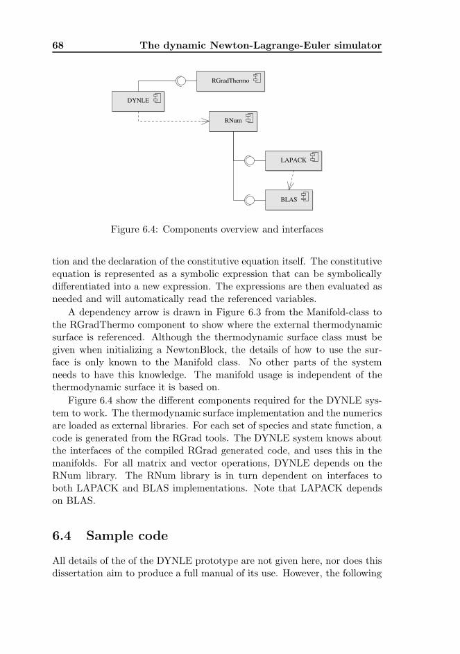
68 The dynamic Newton-Lagrange-Euler simulator
DYNLE
RGradThermo
RNum
BLAS
LAPACK
Figure 6.4: Components overview and interfaces
tion and the declaration of the constitutive equation itself. The constitutiveequation is represented as a symbolic expression that can be symbolicallydifferentiated into a new expression. The expressions are then evaluated asneeded and will automatically read the referenced variables.
A dependency arrow is drawn in Figure 6.3 from the Manifold-class tothe RGradThermo component to show where the external thermodynamicsurface is referenced. Although the thermodynamic surface class must begiven when initializing a NewtonBlock, the details of how to use the sur-face is only known to the Manifold class. No other parts of the systemneeds to have this knowledge. The manifold usage is independent of thethermodynamic surface it is based on.
Figure 6.4 show the different components required for the DYNLE sys-tem to work. The thermodynamic surface implementation and the numericsare loaded as external libraries. For each set of species and state function, acode is generated from the RGrad tools. The DYNLE system knows aboutthe interfaces of the compiled RGrad generated code, and uses this in themanifolds. For all matrix and vector operations, DYNLE depends on theRNum library. The RNum library is in turn dependent on interfaces toboth LAPACK and BLAS implementations. Note that LAPACK dependson BLAS.
6.4 Sample code
All details of the of the DYNLE prototype are not given here, nor does thisdissertation aim to produce a full manual of its use. However, the following
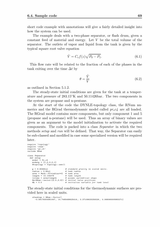
6.4. Sample code 69
short code example with annotations will give a fairly detailed insight intohow the system can be used.
The example deals with a two-phase separator, or flash drum, given aconstant feed of material and energy. Let V be the total volume of theseparator. The outlets of vapor and liquid from the tank is given by thetypical square root valve equation
V = Cvf(z)√
P0 − P1. (6.1)
This flow rate will be related to the fraction of each of the phases in thetank exiting over the time ∆t by
θ =V
V(6.2)
as outlined in Section 5.1.2.The steady-state initial conditions are given for the tank at a temper-
ature and pressure of 283.15K and 50.11426bar. The two components inthe system are propane and n-pentane.
At the start of the code the DYNLE-topology class, the RNum nu-merics and the RGrad thermodynamic model called pr c4 are all loaded.The RGrad model contains more components, but only component 1 and 5(propane and n-pentane) will be used. Thus an array of binary values aregiven as an argument to the model initialization to activate the requiredcomponents. The code is packed into a class Separator in which the twomethods setup and run will be defined. That way, the Separator can easilybe sub-classed and modified in case some specialized version will be requiredlater.require ’topology ’
require ’rnum ’
require ’pr_c4 ’
include RNum
class Separator
def setup
model = Pr_c4
modarg = [1,0,0,0,1]
@topology = Topology ::new ()
g = 9.80665 e1 # standard gravity in scaled units .
radius = 0.84 e1 # tank radius
area = Math ::PI*radius **2 # tank area
length = 10.105076 # tank length
volume = area *length # assume cylindrical shape
@z=RNum ::vector ([0.5 ,0.5]) # initial valve positions
@h = 0.0 # initialize variable for tank level
The steady-state initial conditions for the thermodynamic surfaces are pro-vided here in scaled units.
xfeedvap = RNum ::Vector[
-3.58178304981447 , 14.7485488625416 , 3.27108625259226 , 0.068069305883271]
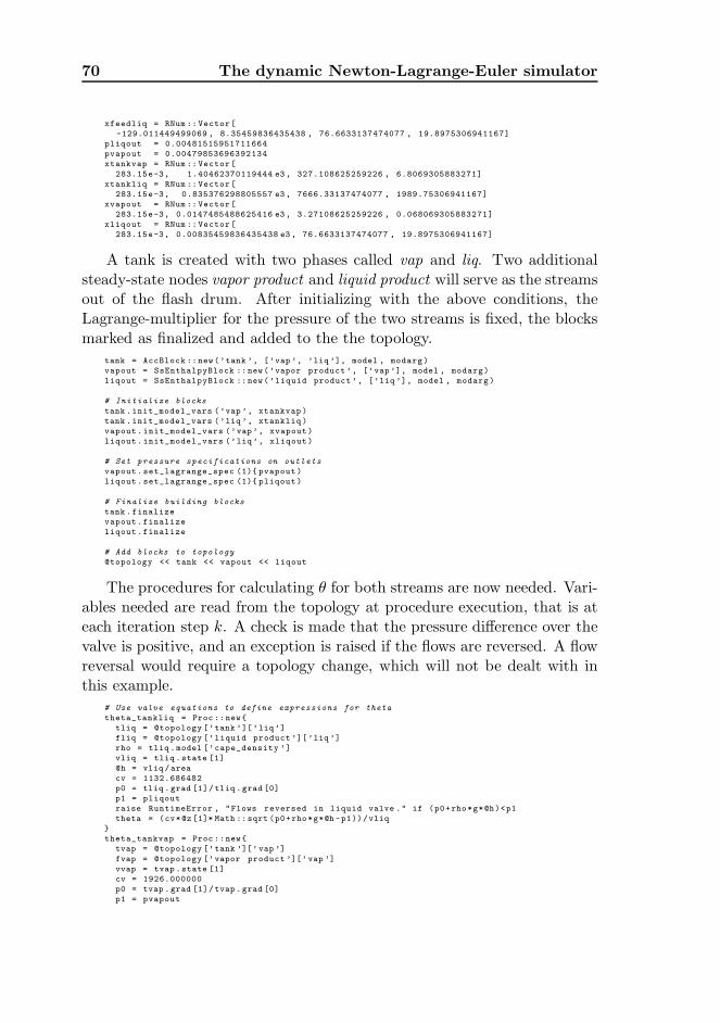
70 The dynamic Newton-Lagrange-Euler simulator
xfeedliq = RNum :: Vector[
-129.011449499069 , 8.35459836435438 , 76.6633137474077 , 19.8975306941167]
pliqout = 0.00481515951711664
pvapout = 0.00479853696392134
xtankvap = RNum :: Vector[
283.15e-3, 1.40462370119444 e3, 327.108625259226 , 6.8069305883271]
xtankliq = RNum :: Vector[
283.15e-3, 0.835376298805557 e3, 7666.33137474077 , 1989.75306941167]
xvapout = RNum :: Vector[
283.15e-3, 0.0147485488625416 e3, 3.27108625259226 , 0.068069305883271]
xliqout = RNum :: Vector[
283.15e-3, 0.00835459836435438 e3 , 76.6633137474077 , 19.8975306941167]
A tank is created with two phases called vap and liq. Two additionalsteady-state nodes vapor product and liquid product will serve as the streamsout of the flash drum. After initializing with the above conditions, theLagrange-multiplier for the pressure of the two streams is fixed, the blocksmarked as finalized and added to the the topology.
tank = AccBlock ::new(’tank ’, [’vap ’, ’liq ’], model , modarg)
vapout = SsEnthalpyBlock ::new(’vapor product ’, [’vap’], model , modarg)
liqout = SsEnthalpyBlock ::new(’liquid product ’, [’liq ’], model , modarg)
# Initialize blocks
tank .init_model_vars (’vap ’, xtankvap )
tank .init_model_vars (’liq ’, xtankliq )
vapout.init_model_vars (’vap’, xvapout)
liqout.init_model_vars (’liq’, xliqout)
# Set pressure specifications on outlets
vapout.set_lagrange_spec (1) pvapout )
liqout.set_lagrange_spec (1) pliqout )
# Finalize building blocks
tank .finalize
vapout.finalize
liqout.finalize
# Add blocks to topology
@topology << tank << vapout << liqout
The procedures for calculating θ for both streams are now needed. Vari-ables needed are read from the topology at procedure execution, that is ateach iteration step k. A check is made that the pressure difference over thevalve is positive, and an exception is raised if the flows are reversed. A flowreversal would require a topology change, which will not be dealt with inthis example.
# Use valve equations to define expressions for theta
theta_tankliq = Proc ::new
tliq = @topology [’tank ’][’liq’]
fliq = @topology [’liquid product ’][’liq ’]
rho = tliq .model [’cape_density ’]
vliq = tliq .state [1]
@h = vliq /area
cv = 1132.686482
p0 = tliq .grad [1]/tliq .grad [0]
p1 = pliqout
raise RuntimeError , "Flows reversed in liquid valve ." if (p0+rho*g*@h)<p1
theta = (cv*@z[1]* Math ::sqrt (p0+rho*g*@h -p1))/vliq
theta_tankvap = Proc ::new
tvap = @topology [’tank ’][’ vap ’]
fvap = @topology [’vapor product ’][’ vap ’]
vvap = tvap .state [1]
cv = 1926.000000
p0 = tvap .grad [1]/tvap .grad [0]
p1 = pvapout
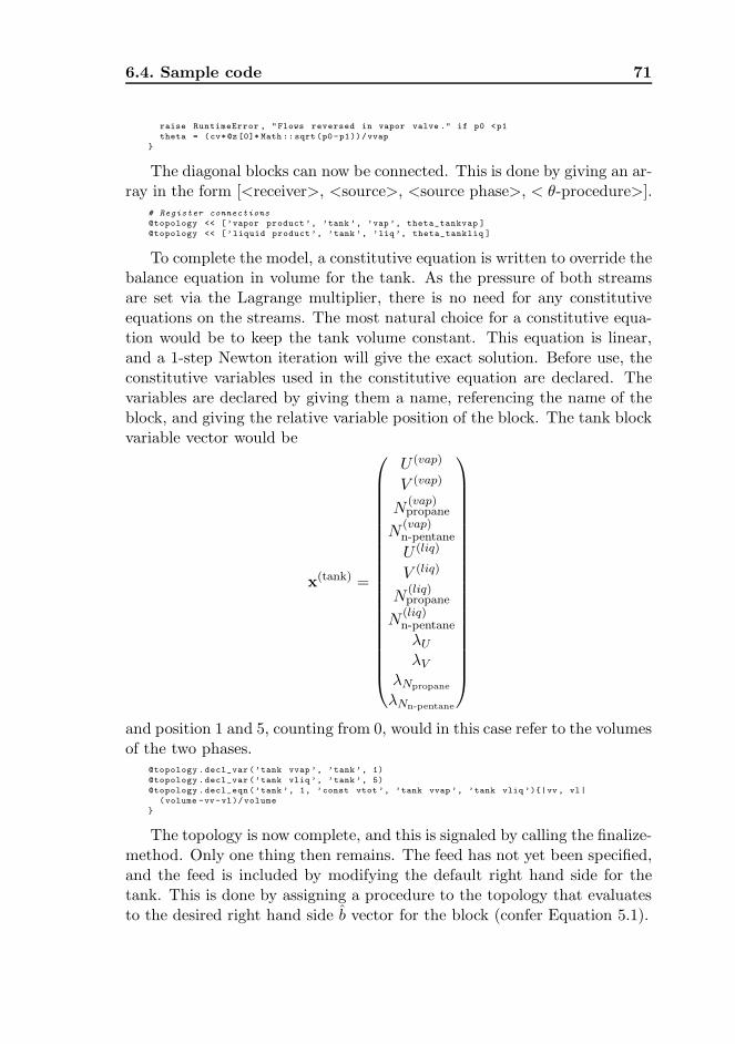
6.4. Sample code 71
raise RuntimeError , "Flows reversed in vapor valve ." if p0 <p1
theta = (cv*@z[0]* Math :: sqrt (p0-p1))/vvap
The diagonal blocks can now be connected. This is done by giving an ar-ray in the form [<receiver>, <source>, <source phase>, < θ-procedure>].
# Register connections
@topology << [’vapor product ’, ’tank ’, ’vap ’, theta_tankvap ]
@topology << [’liquid product ’, ’tank ’, ’liq ’, theta_tankliq ]
To complete the model, a constitutive equation is written to override thebalance equation in volume for the tank. As the pressure of both streamsare set via the Lagrange multiplier, there is no need for any constitutiveequations on the streams. The most natural choice for a constitutive equa-tion would be to keep the tank volume constant. This equation is linear,and a 1-step Newton iteration will give the exact solution. Before use, theconstitutive variables used in the constitutive equation are declared. Thevariables are declared by giving them a name, referencing the name of theblock, and giving the relative variable position of the block. The tank blockvariable vector would be
x(tank) =
U (vap)
V (vap)
N(vap)propane
N(vap)n-pentane
U (liq)
V (liq)
N(liq)propane
N(liq)n-pentane
λU
λV
λNpropane
λNn-pentane
and position 1 and 5, counting from 0, would in this case refer to the volumesof the two phases.
@topology .decl_var (’tank vvap ’, ’tank ’, 1)
@topology .decl_var (’tank vliq ’, ’tank ’, 5)
@topology .decl_eqn (’tank ’, 1, ’const vtot ’, ’tank vvap ’, ’tank vliq ’)|vv , vl|
(volume -vv-vl)/volume
The topology is now complete, and this is signaled by calling the finalize-method. Only one thing then remains. The feed has not yet been specified,and the feed is included by modifying the default right hand side for thetank. This is done by assigning a procedure to the topology that evaluatesto the desired right hand side b vector for the block (confer Equation 5.1).
72 The dynamic Newton-Lagrange-Euler simulator
@topology .finalize
# Set feed in rhs for tank , using a procedure.
@topology [’tank ’]. rhsintmod xfeedvap + xfeedliq
end #def setup
The model is now ready to run:
def run(fd)
t = 0.0
dt = 1.0
tfinal = 2500.0
while t < tfinal
err , dx = @topology .solve
ghaterr , lmgnorm = @topology .update(dx, dt)
@topology .acceptstep (dt)
t += dt
end
end #def run
end #class Separator
Results of a similar model are given in Section 7.1.
Chapter 7
Case studies
Two examples will be presented in this chapter in order to exemplify the usesof the Newton-Lagrange-Euler methodology. The first case is a reimplemen-tation of a model of a dynamic separator found in the literature. A directcomparison of simulation results is made. The second case goes deeper intothe Joule experiment mentioned in Section 4.4, and adds chemical reactionand an isentropic description of the flow.
7.1 A two phase separator
In Section 5.3, simulation results were shown for a simple two-phase vapor-liquid separator to show the effect of time resolution and dynamics on diag-nostics that can be used for step length control. A more detailed descriptionof the separator model and simulation results follows. The separator is areimplementation of the case given by Goncalves et al. [2007], using thedynamic Newton-Lagrange-Euler methodology and developed tools.
The model builds on the same principles as was shown by example inSection 4.3, except that the upstream reservoir and product streams areincluded to the calculation as separate blocks. A conceptual sketch of themodel is shown in Figure 7.1. The reservoir is modeled as a two phasesteady state block in (H,V/T,N)-variables, with a feed given on the righthand side of the Newton-Lagrange-Euler systems of equations. In otherwords, the reservoir is a steady state flash with specified feed. The singledegree of freedom available for this block is used to specify the pressurethrough setting the second Lagrange multiplier. The next two nodes aresimple streams, without any property calculation, in (H,V/T,N)-variableswith a corresponding diagonal block being the identity. If the feed is to bekept at a constant rate and at constant intensive properties, the reservoirs
73
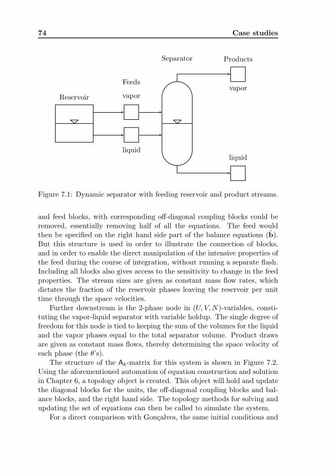
74 Case studies
Reservoir
Feeds
liquid
vapor
Separator Products
vapor
liquid
Figure 7.1: Dynamic separator with feeding reservoir and product streams.
and feed blocks, with corresponding off-diagonal coupling blocks could beremoved, essentially removing half of all the equations. The feed wouldthen be specified on the right hand side part of the balance equations (b).But this structure is used in order to illustrate the connection of blocks,and in order to enable the direct manipulation of the intensive properties ofthe feed during the course of integration, without running a separate flash.Including all blocks also gives access to the sensitivity to change in the feedproperties. The stream sizes are given as constant mass flow rates, whichdictates the fraction of the reservoir phases leaving the reservoir per unittime through the space velocities.
Further downstream is the 2-phase node in (U, V,N)-variables, consti-tuting the vapor-liquid separator with variable holdup. The single degree offreedom for this node is tied to keeping the sum of the volumes for the liquidand the vapor phases equal to the total separator volume. Product drawsare given as constant mass flows, thereby determining the space velocity ofeach phase (the θ’s).
The structure of the Ak-matrix for this system is shown in Figure 7.2.Using the aforementioned automation of equation construction and solutionin Chapter 6, a topology object is created. This object will hold and updatethe diagonal blocks for the units, the off-diagonal coupling blocks and bal-ance blocks, and the right hand side. The topology methods for solving andupdating the set of equations can then be called to simulate the system.
For a direct comparison with Goncalves, the same initial conditions and
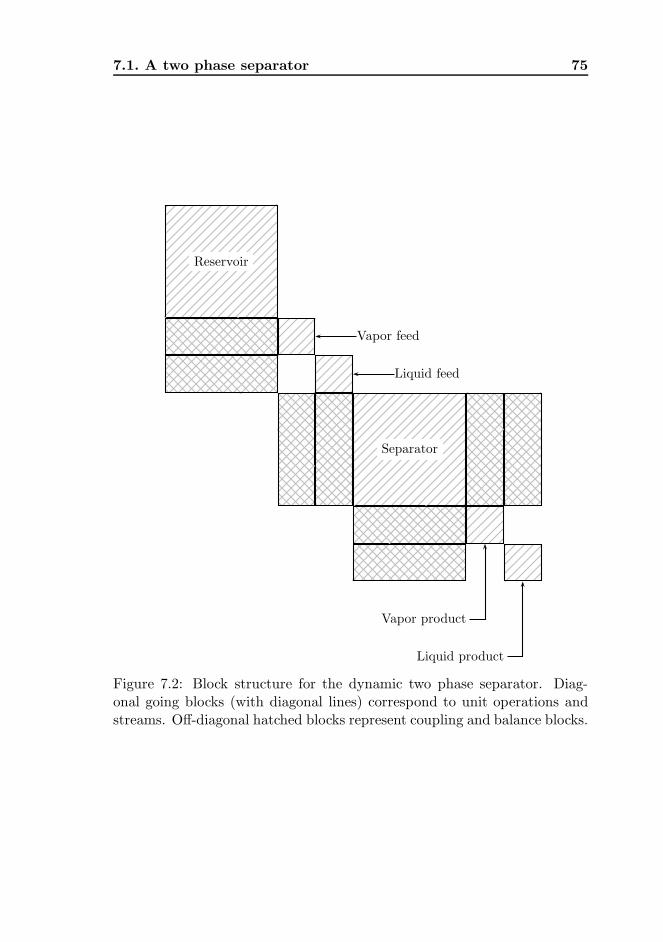
7.1. A two phase separator 75
Reservoir
Vapor feed
Liquid feed
Separator
Vapor product
Liquid product
Figure 7.2: Block structure for the dynamic two phase separator. Diag-onal going blocks (with diagonal lines) correspond to unit operations andstreams. Off-diagonal hatched blocks represent coupling and balance blocks.
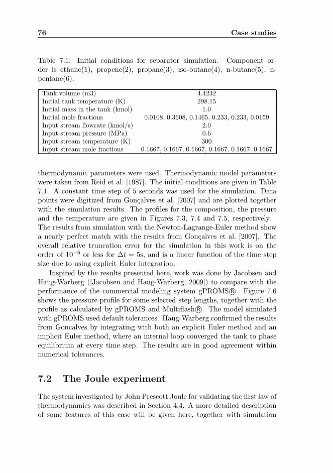
76 Case studies
Table 7.1: Initial conditions for separator simulation. Component or-der is ethane(1), propene(2), propane(3), iso-butane(4), n-butane(5), n-pentane(6).
Tank volume (m3) 4.4232Initial tank temperature (K) 298.15Initial mass in the tank (kmol) 1.0Initial mole fractions 0.0108, 0.3608, 0.1465, 0.233, 0.233, 0.0159Input stream flowrate (kmol/s) 2.0Input stream pressure (MPa) 0.6Input stream temperature (K) 300Input stream mole fractions 0.1667, 0.1667, 0.1667, 0.1667, 0.1667, 0.1667
thermodynamic parameters were used. Thermodynamic model parameterswere taken from Reid et al. [1987]. The initial conditions are given in Table7.1. A constant time step of 5 seconds was used for the simulation. Datapoints were digitized from Goncalves et al. [2007] and are plotted togetherwith the simulation results. The profiles for the composition, the pressureand the temperature are given in Figures 7.3, 7.4 and 7.5, respectively.The results from simulation with the Newton-Lagrange-Euler method showa nearly perfect match with the results from Goncalves et al. [2007]. Theoverall relative truncation error for the simulation in this work is on theorder of 10−6 or less for ∆t = 5s, and is a linear function of the time stepsize due to using explicit Euler integration.
Inspired by the results presented here, work was done by Jacobsen andHaug-Warberg ([Jacobsen and Haug-Warberg, 2009]) to compare with theperformance of the commercial modeling system gPROMS R©. Figure 7.6shows the pressure profile for some selected step lengths, together with theprofile as calculated by gPROMS and Multiflash R©. The model simulatedwith gPROMS used default tolerances. Haug-Warberg confirmed the resultsfrom Goncalves by integrating with both an explicit Euler method and animplicit Euler method, where an internal loop converged the tank to phaseequilibrium at every time step. The results are in good agreement withinnumerical tolerances.
7.2 The Joule experiment
The system investigated by John Prescott Joule for validating the first law ofthermodynamics was described in Section 4.4. A more detailed descriptionof some features of this case will be given here, together with simulation
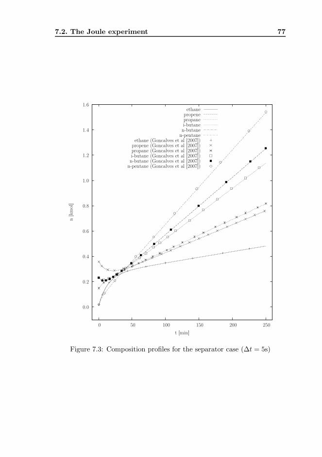
7.2. The Joule experiment 77
0.0
0.2
0.4
0.6
0.8
1.0
1.2
1.4
1.6
0 50 100 150 200 250
n [km
ol]
t [min]
ethanepropenepropanei-butanen-butane
n-pentaneethane (Goncalves et al [2007])
propene (Goncalves et al [2007])propane (Goncalves et al [2007])i-butane (Goncalves et al [2007])n-butane (Goncalves et al [2007])
n-pentane (Goncalves et al [2007])
Figure 7.3: Composition profiles for the separator case (∆t = 5s)
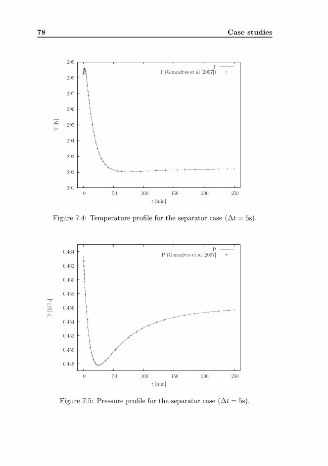
78 Case studies
291
292
293
294
295
296
297
298
299
0 50 100 150 200 250
T [K
]
t [min]
TT (Goncalves et al [2007])
Figure 7.4: Temperature profile for the separator case (∆t = 5s).
0.448
0.450
0.452
0.454
0.456
0.458
0.460
0.462
0.464
0 50 100 150 200 250
P [M
Pa]
t [min]
PP (Goncalves et al [2007]
Figure 7.5: Pressure profile for the separator case (∆t = 5s).
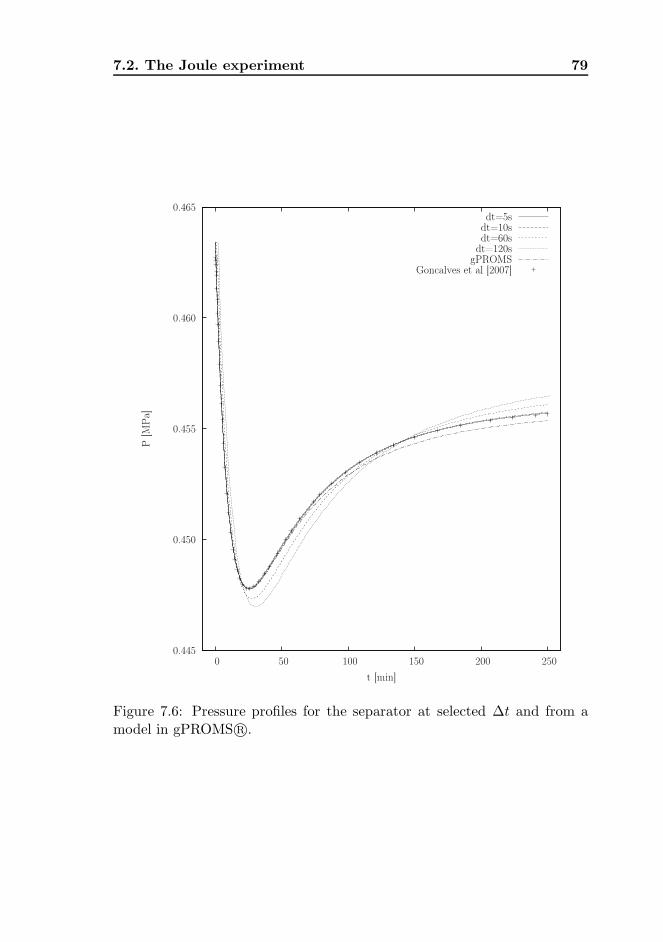
7.2. The Joule experiment 79
0.445
0.450
0.455
0.460
0.465
0 50 100 150 200 250
P [M
Pa]
t [min]
dt=5sdt=10sdt=60s
dt=120sgPROMS
Goncalves et al [2007]
Figure 7.6: Pressure profiles for the separator at selected ∆t and from amodel in gPROMS R©.
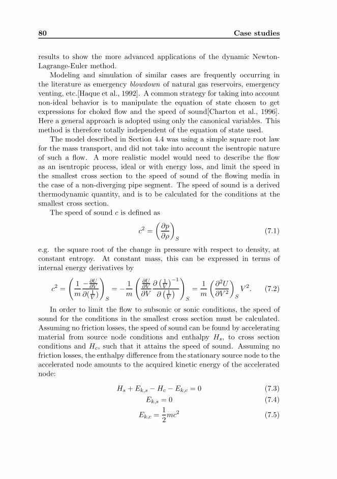
80 Case studies
results to show the more advanced applications of the dynamic Newton-Lagrange-Euler method.
Modeling and simulation of similar cases are frequently occurring inthe literature as emergency blowdown of natural gas reservoirs, emergencyventing, etc.[Haque et al., 1992]. A common strategy for taking into accountnon-ideal behavior is to manipulate the equation of state chosen to getexpressions for choked flow and the speed of sound[Charton et al., 1996].Here a general approach is adopted using only the canonical variables. Thismethod is therefore totally independent of the equation of state used.
The model described in Section 4.4 was using a simple square root lawfor the mass transport, and did not take into account the isentropic natureof such a flow. A more realistic model would need to describe the flowas an isentropic process, ideal or with energy loss, and limit the speed inthe smallest cross section to the speed of sound of the flowing media inthe case of a non-diverging pipe segment. The speed of sound is a derivedthermodynamic quantity, and is to be calculated for the conditions at thesmallest cross section.
The speed of sound c is defined as
c2 =
(∂p
∂ρ
)
S
(7.1)
e.g. the square root of the change in pressure with respect to density, atconstant entropy. At constant mass, this can be expressed in terms ofinternal energy derivatives by
c2 =
(
1
m
− ∂U∂V
∂( 1V )
)
S
= − 1
m
(∂U∂V
∂V
∂(
1V
)−1
∂(
1V
)
)
S
=1
m
(∂2U
∂V 2
)
S
V 2. (7.2)
In order to limit the flow to subsonic or sonic conditions, the speed ofsound for the conditions in the smallest cross section must be calculated.Assuming no friction losses, the speed of sound can be found by acceleratingmaterial from source node conditions and enthalpy Hs, to cross sectionconditions and Hc, such that it attains the speed of sound. Assuming nofriction losses, the enthalpy difference from the stationary source node to theaccelerated node amounts to the acquired kinetic energy of the acceleratednode:
Hs + Ek,s −Hc − Ek,c = 0 (7.3)
Ek,s = 0 (7.4)
Ek,c =1
2mc2 (7.5)
7.2. The Joule experiment 81
A copy of the source node is represented with the energy function U as afunction of (S, V,N). Keeping entropy and mass constant, the volume isincreased until the following relations are satisfied
Hs = Us +∂Ss
∂Vs
(∂Ss
∂Us
)−1
Vs (7.6)
Hc : Vc 7→∂Uc
∂ScSc+ <
∂Uc
∂Nc
,Nc > (7.7)
Ek,c : Vc 7→1
2
(∂2Uc
∂V 2c
)
S
V 2c (7.8)
f : Vc 7→ Hs −Hc − Ek,c (7.9)
f = 0 (7.10)
where subscripts s and c refers to the source and accelerated node, respec-tively. By adding to the Newton-Lagrange-Euler system of equations theconstitutive equation f = 0 and the derivative of f with respect to thevolume Vc,
(∂f
∂Vc
)
S,N
= − ∂2Uc
∂Sc∂VcSc− <
∂2Uc
∂Nc∂Vc,Nc > −1
2
∂3Uc
∂V 3c
+∂2Uc
∂V 2c
Vc, (7.11)
the accelerated node will track the speed of sound at the accelerated state.A second copy, or slave node, of the source node is used to find the
speed in the smallest cross section based on the change in specific enthalpyfrom the source node to the receiver node. This uses the U(S, V,N) energyfunction in order to conserve entropy and mass. The one degree of freedomis used to manipulate V such that the node is kept at the pressure of thereceiver node. By noting that the derivative (∂U/∂V )S,N = −p, the pressurecan be set directly by specifying the second Lagrange multiplier of this nodein the Newton-Lagrange-Euler equation system. In essence, the node actsas an isentropic valve. Knowing the change in specific enthalpy from thesource to this valve node, and the cross section area, the linear speed canbe calculated by
v =√
2∆h. (7.12)
The speed v is then compared to the speed of sound c of the acceleratedcopy of the source node, in order to ensure that the speed is at a maximumvalue of the speed of sound as described in the former paragraph. In otherwords, a maximum of Mach 1 is allowed. Given the speed and cross sectionarea, the mass and energy flow from the source node to the receiver node iscalculated.
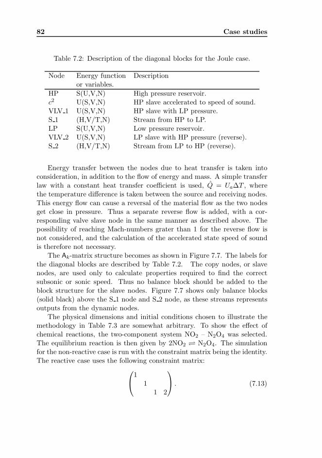
82 Case studies
Table 7.2: Description of the diagonal blocks for the Joule case.
Node Energy function Descriptionor variables.
HP S(U,V,N) High pressure reservoir.c2 U(S,V,N) HP slave accelerated to speed of sound.VLV 1 U(S,V,N) HP slave with LP pressure.S 1 (H,V/T,N) Stream from HP to LP.LP S(U,V,N) Low pressure reservoir.VLV 2 U(S,V,N) LP slave with HP pressure (reverse).S 2 (H,V/T,N) Stream from LP to HP (reverse).
Energy transfer between the nodes due to heat transfer is taken intoconsideration, in addition to the flow of energy and mass. A simple transferlaw with a constant heat transfer coefficient is used, Q = Ua∆T , wherethe temperature difference is taken between the source and receiving nodes.This energy flow can cause a reversal of the material flow as the two nodesget close in pressure. Thus a separate reverse flow is added, with a cor-responding valve slave node in the same manner as described above. Thepossibility of reaching Mach-numbers grater than 1 for the reverse flow isnot considered, and the calculation of the accelerated state speed of soundis therefore not necessary.
The Ak-matrix structure becomes as shown in Figure 7.7. The labels forthe diagonal blocks are described by Table 7.2. The copy nodes, or slavenodes, are used only to calculate properties required to find the correctsubsonic or sonic speed. Thus no balance block should be added to theblock structure for the slave nodes. Figure 7.7 shows only balance blocks(solid black) above the S 1 node and S 2 node, as these streams representsoutputs from the dynamic nodes.
The physical dimensions and initial conditions chosen to illustrate themethodology in Table 7.3 are somewhat arbitrary. To show the effect ofchemical reactions, the two-component system NO2 – N2O4 was selected.The equilibrium reaction is then given by 2NO2 N2O4. The simulationfor the non-reactive case is run with the constraint matrix being the identity.The reactive case uses the following constraint matrix:
11
1 2
. (7.13)
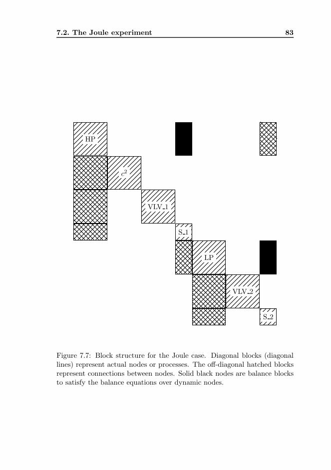
7.2. The Joule experiment 83
HP
c2
VLV 1
S 1
LP
VLV 2
S 2
Figure 7.7: Block structure for the Joule case. Diagonal blocks (diagonallines) represent actual nodes or processes. The off-diagonal hatched blocksrepresent connections between nodes. Solid black nodes are balance blocksto satisfy the balance equations over dynamic nodes.
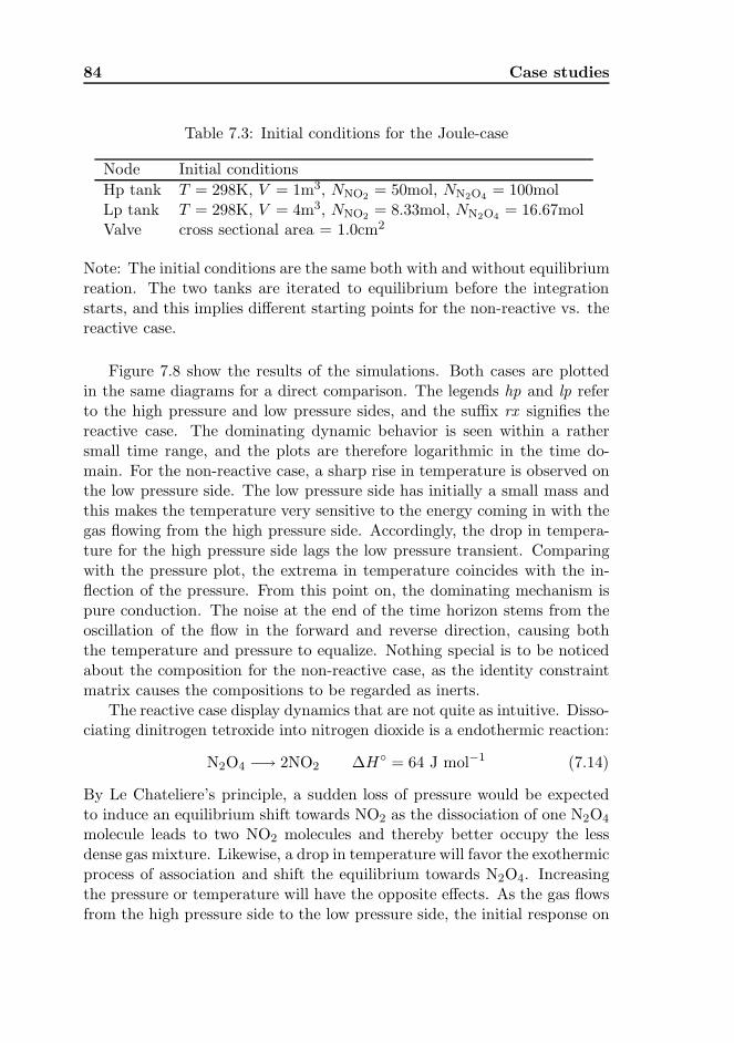
84 Case studies
Table 7.3: Initial conditions for the Joule-case
Node Initial conditions
Hp tank T = 298K, V = 1m3, NNO2 = 50mol, NN2O4 = 100molLp tank T = 298K, V = 4m3, NNO2 = 8.33mol, NN2O4 = 16.67molValve cross sectional area = 1.0cm2
Note: The initial conditions are the same both with and without equilibriumreation. The two tanks are iterated to equilibrium before the integrationstarts, and this implies different starting points for the non-reactive vs. thereactive case.
Figure 7.8 show the results of the simulations. Both cases are plottedin the same diagrams for a direct comparison. The legends hp and lp referto the high pressure and low pressure sides, and the suffix rx signifies thereactive case. The dominating dynamic behavior is seen within a rathersmall time range, and the plots are therefore logarithmic in the time do-main. For the non-reactive case, a sharp rise in temperature is observed onthe low pressure side. The low pressure side has initially a small mass andthis makes the temperature very sensitive to the energy coming in with thegas flowing from the high pressure side. Accordingly, the drop in tempera-ture for the high pressure side lags the low pressure transient. Comparingwith the pressure plot, the extrema in temperature coincides with the in-flection of the pressure. From this point on, the dominating mechanism ispure conduction. The noise at the end of the time horizon stems from theoscillation of the flow in the forward and reverse direction, causing boththe temperature and pressure to equalize. Nothing special is to be noticedabout the composition for the non-reactive case, as the identity constraintmatrix causes the compositions to be regarded as inerts.
The reactive case display dynamics that are not quite as intuitive. Disso-ciating dinitrogen tetroxide into nitrogen dioxide is a endothermic reaction:
N2O4 −→ 2NO2 ∆H = 64 J mol−1 (7.14)
By Le Chateliere’s principle, a sudden loss of pressure would be expectedto induce an equilibrium shift towards NO2 as the dissociation of one N2O4
molecule leads to two NO2 molecules and thereby better occupy the lessdense gas mixture. Likewise, a drop in temperature will favor the exothermicprocess of association and shift the equilibrium towards N2O4. Increasingthe pressure or temperature will have the opposite effects. As the gas flowsfrom the high pressure side to the low pressure side, the initial response on
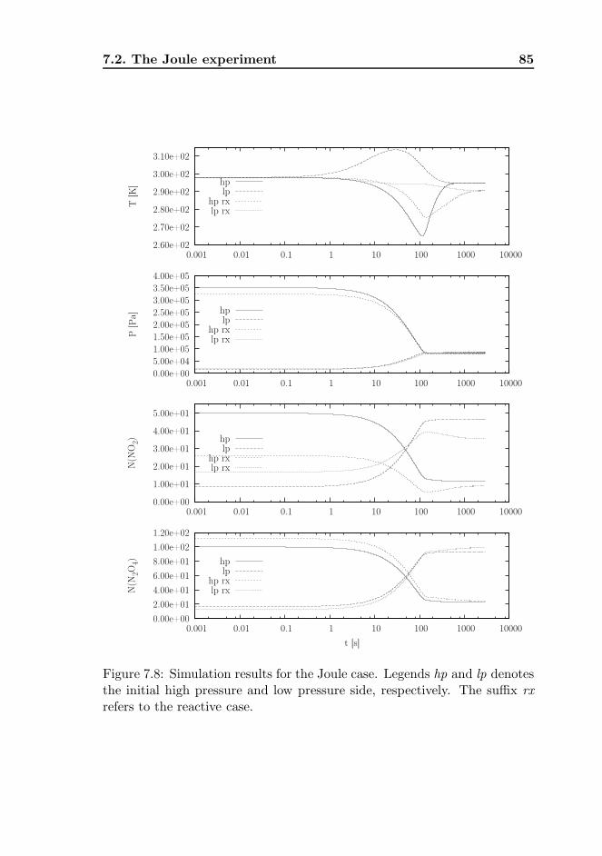
7.2. The Joule experiment 85
2.60e+02
2.70e+02
2.80e+02
2.90e+02
3.00e+02
3.10e+02
0.001 0.01 0.1 1 10 100 1000 10000
T [K
] hplp
hp rxlp rx
0.00e+00
5.00e+04
1.00e+05
1.50e+05
2.00e+05
2.50e+05
3.00e+05
3.50e+05
4.00e+05
0.001 0.01 0.1 1 10 100 1000 10000
P [P
a]
hplp
hp rxlp rx
0.00e+00
1.00e+01
2.00e+01
3.00e+01
4.00e+01
5.00e+01
0.001 0.01 0.1 1 10 100 1000 10000
N(N
O2) hp
lphp rxlp rx
0.00e+00
2.00e+01
4.00e+01
6.00e+01
8.00e+01
1.00e+02
1.20e+02
0.001 0.01 0.1 1 10 100 1000 10000
N(N
2O4)
t [s]
hplp
hp rxlp rx
Figure 7.8: Simulation results for the Joule case. Legends hp and lp denotesthe initial high pressure and low pressure side, respectively. The suffix rxrefers to the reactive case.
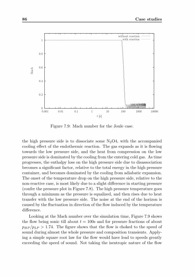
86 Case studies
0
0.2
0.4
0.6
0.8
1
0.001 0.01 0.1 1 10 100 1000 10000
Mac
h
t [s]
without reactionwith reaction
Figure 7.9: Mach number for the Joule case.
the high pressure side is to dissociate some N2O4, with the accompaniedcooling effect of the endothermic reaction. The gas expands as it is flowingtowards the low pressure side, and the heat from compression on the lowpressure side is dominated by the cooling from the entering cold gas. As timeprogresses, the enthalpy loss on the high pressure side due to disassociationbecomes a significant factor, relative to the total energy in the high pressurecontainer, and becomes dominated by the cooling from adiabatic expansion.The onset of the temperature drop on the high pressure side, relative to thenon-reactive case, is most likely due to a slight difference in starting pressure(confer the pressure plot in Figure 7.8). The high pressure temperature goesthrough a minimum as the pressure is equalized, and then rises due to heattransfer with the low pressure side. The noise at the end of the horizon iscaused by the fluctuation in direction of the flow induced by the temperaturedifference.
Looking at the Mach number over the simulation time, Figure 7.9 showsthe flow being sonic till about t = 100s and for pressure fractions of aboutpHP /pLP > 1.74. The figure shows that the flow is choked to the speed ofsound during almost the whole pressure and composition transients. Apply-ing a simple square root law for the flow would have lead to speeds greatlyexceeding the speed of sound. Not taking the isentropic nature of the flow
7.2. The Joule experiment 87
into account is thus a serious modeling error even for pressure drops withthe ratio of pressures p1/p2 = 2.

88 Case studies
Chapter 8
Concluding remarks
The success of Siepmann [2006] and his steady-state simulator concept basedon a canonical basis has inspired the search for finding a similar methodologythat could work for simulating dynamic systems.
The review of the properties of thermodynamic functions and the use ofthe Legendre transforms and Massieu functions on thermodynamic poten-tials resulted in the definition of the thermodynamic surface and manifoldin Chapter 2. The explicitly defined thermodynamic potential, the ther-modynamic surface, is mapped into a thermodynamic manifold under theLegendre transform and Massieu function. However, only local propertiesare known on the thermodynamic manifold. Tracing the manifold requiresiteration in the variables of the surface. For small changes, the manifoldcan be approximated with local derivatives. These abstractions yield insightinto the challenges involved when calculating the update of thermodynamicproperties that are implicitly defined. By using derivative information, theupdate of the surface variables from a shift in manifold variables can beapproximated by a linear mapping.
Solving for phase and reaction equilibrium can be viewed as an opti-mization problem where the objective is to find the extremal value on aconstrained thermodynamic manifold. Which manifold to use is a mat-ter of choice. With proper derivative information available, the Legendretransform and Massieu function can be applied to map coordinates on athermodynamic surface to a thermodynamic manifold on which the con-straints will be linear. With linear constraints the search for the optimumis greatly simplified. The variables of the manifold on which a given problemwill be linearly constrained are defined as the problem canonical variables.
An equilibrium problem such as a phase separator, reactor or other unitoperation can be viewed as a node in the process flow sheet. Nodes can be
89
90 Concluding remarks
aggregated by coupling mass and energy balances in order to describe thecomplete process. The dynamic Newton-Lagrange-Euler formulation intro-duced in Chapter 4, and further refined in Chapter 5, can be used to modeland simulate whole process flow sheets. Each node is supposedly describedin its natural canonical variables, and thus the basic balance equations arekept linear. Other constraints, not necessarily linear, are approximated bylinearization using symbolic derivatives. As the thermodynamic state in-volves Nc + 2 variables, while most processes only involve balances on massand energy, each node will have one degree of freedom that needs to bespecified in order to close the equations. This is achieved through addingconstitutive equations that manipulate slack variables. As an example, atank with variable holdup will typically have the constraint of constant totalvolume. Thus the constitutive equation will be such that the slack variableis adjusted to keep the volume constant. For constraints that can be relatedto a linear mapping of the Lagrange-multipliers, the degree of freedom isspecified by fixing the value of the Lagrange-multiplier of the node.
The dynamic Newton-Lagrange-Euler formulation gives a linear equa-tion system Ax = b to be solved at every iteration. The block diagonal of A
is related to the equations for each node. Off-diagonal blocks are introducedin order to allow the exchange of mass and energy between nodes. Lowerdiagonal blocks transfer mass and energy from one node to another nodefurther down along the block diagonal. Upper diagonal blocks connect toa node further up on the block diagonal. By using Jacobian matrices, theconnected nodes can be described in a possibly different set of canonicalvariables. When transferring mass and energy from a node with holdup,the off-diagonal connection block includes a scaling factor that is directlyrelated to the fraction of the original holdup that exits during an integrationtime step. This fraction is the space velocity of the holdup node. The spacevelocity is calculated from an auxiliary procedure, such as a valve equation.
A software system was designed and implemented to automate the con-struction and updating of the equations in the dynamic Newton-Lagrange-Euler formulation for any given set of nodes making up a process flowsheet. With this tool, two case studies have been explored. The first casestudy re-implements a model given in the literature for direct comparisonof simulation results. The model in the Newton-Lagrange-Euler formula-tion is capable of reproducing the literature data perfectly. The secondcase study explores the possibilities for more advanced models with thedynamic Newton-Lagrange-Euler formulation and the availability of higherorder derivatives on manifolds. The model investigates the famous Jouleexperiment from 1843 for a blow down from a high pressure reservoir to a
91
low pressure reservoir with choked flow. The case is simulated both withand without reaction equilibrium.
The intent of this work has not been to create a prototype for direct com-parison with established simulation methodologies and commercial prod-ucts. As stated in the introduction, the work has been driven by the ideaof exploring the properties and structure of thermodynamic functions. Thegoal has been to find a simple formulation for the modeling and simulationof dynamic processes with both phase and reaction equilibrium. Throughthe case studies it has been shown that the dynamic Newton-Lagrange-Eulerformulation is capable of simulating simple phase equilibrium problems, aswell as and more advanced phase and reaction equilibrium problems.
Although important, emphasis has not been on finding implicit formu-lations to the integration problem, nor on finding efficient step length al-gorithms. However, diagnostics and normed quantities are suggested thatcan be used for this purpose. Further work is required in order to establishefficient methods for integration. Also, little attention has been given tothe problem of testing the phase assembly for stability, nor the case of largesystems with strongly cyclic processes. These topics should be investigatedfurther.
As this work shows, a systematic approach to the process modeling offlow sheets on a canonical thermodynamic basis is indeed possible. Thisformulation has some promising benefits compared to traditional approachesbased on a single choice of iteration variables.

92 Concluding remarks
Bibliography
Benjamin Andrew Allan. A More Reusable Modeling System. PhD thesis,Carnegie Mellon University, Pittsburgh, PA USA, April 1997.
E. Anderson, Z. Bai, C. Bischof, S. Blackford, J. Demmel, J. Don-garra, J. Du Croz, A. Greenbaum, S. Hammarling, A. McKenney, andD. Sorensen. LAPACK Users’ Guide. Society for Industrial and AppliedMathematics, Philadelphia, PA, third edition, 1999. ISBN 0-89871-447-8(paperback).
V. I. Arnold. Mathematical Methods of Classical Mechanics (Graduate Textsin Mathematics). Springer, September 1989. ISBN 0387968903. URLhttp://www.worldcat.org/isbn/0387968903.
Lorenz T. Biegler. Systematic methods of chemical process design. PrenticeHall PTR, Upper Saddle River, N.J., 1997.
L. S. Blackford, J. Demmel, J. Dongarra, I. Du, S. Hammarling, G. Henry,M. Heroux, L. Kaufman, A. Lumsdaine, A. Petitet, R. Pozo, K. Rem-ington, and R. C. Whaley. An updated set of basic linear algebra sub-programs (blas). ACM Transactions on Mathematical Software, 28(2):135–151, 2002. ISSN 0098-3500.
Grady Booch, Ivar Jacobson, and Jim Rumbaugh. OMG Uni-fied Modeling Language Specification. Object ManagementGroup, Version 1.3, Fifth edition edition, 3 2000. URLhttp://www.omg.org/docs/formal/00-03-01.pdf.
K. E. Brenan, S. L. Campell, and L. R. Petzold. Numerical solution ofinitial-value problems in differential-algebraic equations. North-Holland,New York, 1989.
Egil Brendsdal. Computation of phase equilibria in fluid mixtures. PhDthesis, Høgskolen i Telemark, Norway, Porsgrunn, 1999.
93

94 Bibliography
Herbert B. Callen. Thermodynamics and an introduction to thermostatis-tics. Number 2nd ed. Wiley, New York, 1985.
Stephen L. Campbell and C. William Gear. The index of general nonlin-ear daes. Numerische Mathematik, 72(2):173–196, December 1995. URLhttp://dx.doi.org/10.1007/s002110050165.
Marcelo Castier. Solution of the isochoric-isoenergetic flashproblem by direct entropy maximization. Fluid PhaseEquilibria, 276(1):7 – 17, 2009. ISSN 0378-3812. URLhttp://dx.doi.org/10.1016/j.fluid.2008.10.005.
Jaime Castillo and Ignacio E. Grossmann. Computation ofphase and chemical equilibria. Computers & Chemical En-gineering, 5(2):99 – 108, 1981. ISSN 0098-1354. URLhttp://dx.doi.org/10.1016/0098-1354(81)87005-6.
S. Charton, V. Blet, and J. P. Corriou. A simplified model for real gasexpansion between two reservoirs connected by a thin tube. Chemi-cal Engineering Science, 51(2):295 – 308, 1996. ISSN 0009-2509. URLhttp://dx.doi.org/10.1016/0009-2509(95)00256-1.
F. M. Goncalves, M. Castier, and O. Q. F. Araujo. Dynamic sim-ulation of flash drums using rigorous physical property calculations.Brazilian Journal of Chemical Engineering, 24:277–286, 2007. URLhttp://dx.doi.org/10.1590/S0104-66322007000200012.
E. Hairer, Norsett S. P., and G. Wanner. Solving Ordinary, DifferentialEquations II. Stiff and Differential-Algebraic Problems, volume 2. 2Ed.Springer-Verlag, 2002, 2002. ISBN 3-540-60452-9. Index.
M. A. Haque, S. M. Richardson, and G. Saville. Blowdown of pressurevessels. 1. computer model. Trans IChemE, 70, Part B, 1992.
Tore Haug-Warberg. Computation of thermodynamic equilibria. PhD thesis,Norwegian Institute of Technology, Trondheim, Trondheim, 1988.
Tore Haug-Warberg. On the principles of thermodynamic modeling. InAndrzej Kraslawski and Ilkka Turunen, editors, European Symphosiumon Computer Aided Process Engineering – 13, volume 14. Elsevier, 2003.
Tore Haug-Warberg. Oral session, 2006.
Bibliography 95
Nicholas J. Higham. Accuracy and Stability of Numerical Algorithms. So-ciety for Industrial and Applied Mathematics, Philadelphia, PA, USA,2002. ISBN 0898715210.
M. Hillestad and T. Hertzberg. Dynamic simulation of chemical engineeringsystems by the sequential modular approach. Computers & ChemicalEngineering, 10(4):377 – 388, 1986. ISSN 0098-1354.
Alan C. Hindmarsh, Peter N. Brown, Keith E. Grant, Steven L. Lee, RaduSerban, Dan E. Shumaker, and Carol S. Woodward. SUNDIALS: Suiteof nonlinear and differential/algebraic equation solvers. ACM Transac-tions on Mathematical Software, 31(3):363–396, September 2005. URLhttp://doi.acm.org/10.1145/1089014.1089020.
V. Hlavacek. Analysis of a complex plant-steady state and transient be-havior. Computers & Chemical Engineering, 1(1):75–100, 1977. ISSN0098-1354.
Magnus Glosli Jacobsen and Tore Haug-Warberg. Private communication,2009.
James Prescott Joule. The scientific papers of James Prescott Joule. ThePhysical Society of London, Tailor and Francis, London, 1884.
Peter Kunkel. Differential-algebraic equations: analysis and numerical so-lution. European Mathematical Society, 2006.
Bjørn Tore Løvfall. Computer Realization of Thermodynamic Models Us-ing Algebraic Objects. PhD thesis, Norwegian University of Science andTechnology, 2008.
Yukihiro Matsumoto. Ruby in a Nutshell: A Desktop Quick Reference. ANutshell handbook. 2002. ISBN 0-596-00214-9. Translated from Japaneseby David L. Reynolds, Jr.
Michael L. Michelsen. The isothermal flash problem. part i. stability.Fluid Phase Equilibria, 9(1):1 – 19, 1982. ISSN 0378-3812. URLhttp://dx.doi.org/10.1016/0378-3812(82)85001-2.
Havard Ingvald Moe. Dynamic Process Simulation, Studies on Modelingand Index Reduction. PhD thesis, University of Trondheim, 1995.
Jorge Nocedal. Numerical Optimization. Springer-Verlag New York, Inc.,New York, NY, 1999.
96 Bibliography
Robert C. Reid, John M. Prausnitz, and Bruce E. Poling. The propertiesof gases and liquids. McGraw-Hill, New York, 4th edition, 1987.
Warren D. Seider and Soemantri Widagdo. Multiphase equilibria of reactivesystems. Fluid Phase Equilibria, 123(1-2):283 – 303, 1996. ISSN 0378-3812.
Volker Siepmann. Process modelling on a canonical basis. PhD thesis,Norwegian University of Science and Technology NTNU, 2006.
Robert D. Skeel. Scaling for numerical stability in gaussian elimination. J.ACM, 26(3):494–526, 1979. ISSN 0004-5411.
W. B. White, S. M. Johnson, and G. B. Dantzig. Chemical equilibriumin complex mixtures. The Journal of Chemical Physics, 28(5):751–755,1958. URL http://dx.doi.org/10.1063/1.1744264.
Appendix A
The Ruby numerical library
– RNum
Various third party libraries for the Ruby language offers support for basiclinear algebra. But the lack of a non-limiting license and/or interoperabilitywith standard tools such as BLAS and LAPACK inspired the developmentof a new linear algebra library. The library was named Ruby NumericalLibrary – RNum. The RNum library was released under an Open Sourcelicense at http://rnum.rubyforge.org
A.1 Design and implementation
The basic idea was to make BLAS and LAPACK functions available in theRuby language, using a Ruby-like approach to the interface. The RNumlibrary should also have the possibility of doing in-memory operations wherepossible, eliminating the duplication of function arguments as found in e.g.Matlab. And finally, a clear distinction should be made between scalars, vec-tors and matrices. The latter requirement stems from the authors experiencewith Matlab and similar environments that do not make this distinction.Hence, hard to find bugs are often produced by unintended products reduc-ing to scalars, or the constant worry about whether a vector is representedas a one column or one row matrix.
A set of files were written in the language C to handle storage andmanipulation of the numeric data, and enable calling of BLAS and LAPACKsubroutines. These files constitute the RNum C library. The C library has afunction oriented approach and holds no state. All object oriented featuresof the library were implemented in pure Ruby code. This separation of purefunctions in the C library and object orientation in the Ruby code opens
97
98 The Ruby numerical library – RNum
the C library for possible other uses; the C library might be used directlyto hold matrix storage objects, without the separation into scalars, vectorsand matrices.
A.2 Features
The high level Ruby interface, named RNum, handles all basic linear al-gebra operations. Parts of the LAPACK suite is supported as well, andfull support of all LAPACK features are planned. A total of 234 differentoperations are available in RNum. A short description of some of themfollows.
As mentioned, the separation into scalar, vector and matrix require theuser to be somewhat more stringent when defining them. The scalar type usethe built in numeric type of Ruby and is only used for proper polymorphicbehavior and type coercion. As an example, a product of two vectors usingthe asterisk symbol ∗ represents the inner or dot product and gives a scalarresult. Multiplying a vector with a matrix should fail, as the operationis not properly defined. However, the product of a vector, converted intoa one row matrix, with a matrix is allowed. This would be equivalentto the Matlab/octave v’*m product. In RNum, the vector v, must first beconverted into a row matrix by applying its .row method like this: v.row*m.This product would yield a one row matrix.
Some notable other features are
• the outer product or dyad.
• the rank2 outer product, again in Matlab/octave notation: u*v’ +
v*u’.
• the colon method, where a.colon(b) returns∑
i
∑
j ai,j ∗ bi,j.
One of the Ruby language strengths are its iterator concept and anony-mous functions - aka lambda expressions. The RNum library supports theseconstructs by implementing vector and matrix iterators for efficient elementaccess and manipulation. One argument for creating the RNum library wasto enable in-memory operation. The methods doing in-memory operationsand thereby changing the original object, are given an exclamation markpostfix to the method name. This is a convention in Ruby. To illustrate theiterator and in memory manipulation, the following code will generate a 2x3identity matrix, exchange the elements with random numbers, and set allnumbers greater than 0.2 to zero. All this is done without using temporarystorage.
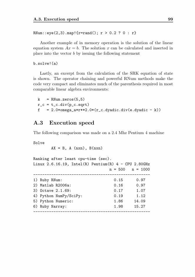
A.3. Execution speed 99
RNum::eye(2,3).map!r=rand(); r > 0.2 ? 0 : r
Another example of in memory operation is the solution of the linearequation system Ax = b. The solution x can be calculated and inserted inplace into the vector b by issuing the following statement
b.solve!(a)
Lastly, an excerpt from the calculation of the SRK equation of stateis shown. The operator chaining and powerful RNum methods make thecode very compact and eliminates much of the parenthesis required in mostcomparable linear algebra environments:
k = RNum.zeros(5,5)
r_c = t_c.div(p_c.sqrt)
f = 2.0*omega_a*r**2.0*(r_c.dyadic.div(e.dyadic - k))
A.3 Execution speed
The following comparison was made on a 2.4 Mhz Pentium 4 machine
Solve
AX = B, A (nxn), B(nxn)
Ranking after least cpu-time (sec).
Linux 2.6.16.19, Intel(R) Pentium(R) 4 - CPU 2.80GHz
n = 500 n = 1000
----------------------------------------------------
1) Ruby RNum: 0.15 0.97
2) Matlab R2006a: 0.16 0.97
3) Octave 2.1.69: 0.17 1.07
4) Python NumPy/SciPy: 0.19 1.12
5) Python Numeric: 1.86 14.09
6) Ruby Narray: 1.98 15.27
----------------------------------------------------

100 The Ruby numerical library – RNum
Appendix B
Jacobian, gradient and
Hessian of thermodynamic
manifolds
The derivation of the properties of some manifolds based on any thermo-dynamic surface in Helmholtz energy will be shown here. Note that thesecond derivative, the Hessian, by definition must be symmetric. Hence,the Hessian can be factored into a congruence product H = LALT.
Some general definitions used in the following sections are given bellow.
U(S, V,N) =
(∂U
∂S
)
V,N
S +
(∂U
∂V
)
S,N
V +
(∂U
∂N
)
S,V
N (B.1)
A(T, V,N) = LS [U(S, V,N)]
= U(S, V,N) −(
∂U
∂S
)
V,N
S = U(S, V,N) − TS (B.2)
101
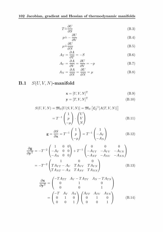
102 Jacobian, gradient and Hessian of thermodynamic manifolds
T =∂U
∂S(B.3)
p=− ∂U
∂V(B.4)
µ=∂U
∂N(B.5)
AT =∂A
∂T= −S (B.6)
AV =∂A
∂V=
∂U
∂V= −p (B.7)
AN =∂A
∂N=
∂U
∂N= µ (B.8)
B.1 S(U, V, N)-manifold
x = [U, V,N ]T (B.9)
y = [T, V,N ]T (B.10)
S(U, V,N) = MS [U(S, V,N)] = MS
[L−1T [A(T, V,N)]
]
= T−1
1p−µ
·
UVN
(B.11)
g =∂S
∂x= T−1
1p−µ
= T−1
1−AV
−AN
(B.12)
∂g
∂yT= −T−2
1 0 0−AV 0 0−AN 0 0
+ T−1
0 0 0−AV T −AV V −AV N
−ANT −ANV −ANN
= −T−2
1 0 0TAV T −AV TAV V TAV N
TANT −AN TANV TANN
(B.13)
∂x
∂yT=
−TATT AV − TATV AN − TATN
0 1 00 0 1
=
−T AV AN
0 1 00 0 1
ATT ATV ATN
0 1 00 0 1
(B.14)
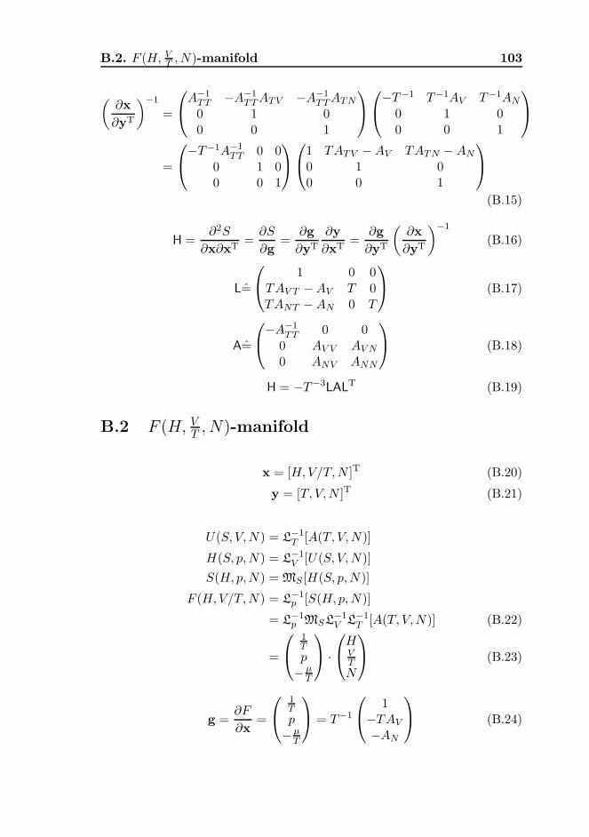
B.2. F (H, VT , N)-manifold 103
(∂x
∂yT
)−1
=
A−1TT −A−1
TT ATV −A−1TTATN
0 1 00 0 1
−T−1 T−1AV T−1AN
0 1 00 0 1
=
−T−1A−1TT 0 0
0 1 00 0 1
1 TATV −AV TATN −AN
0 1 00 0 1
(B.15)
H =∂2S
∂x∂xT=
∂S
∂g=
∂g
∂yT
∂y
∂xT=
∂g
∂yT
(∂x
∂yT
)−1
(B.16)
L=
1 0 0TAV T −AV T 0TANT −AN 0 T
(B.17)
A=
−A−1TT 0 0
0 AV V AV N
0 ANV ANN
(B.18)
H = −T−3LALT (B.19)
B.2 F (H, VT , N)-manifold
x = [H,V/T,N ]T (B.20)
y = [T, V,N ]T (B.21)
U(S, V,N) = L−1T [A(T, V,N)]
H(S, p,N) = L−1V [U(S, V,N)]
S(H, p,N) = MS [H(S, p,N)]
F (H,V/T,N) = L−1p [S(H, p,N)]
= L−1p MSL
−1V L
−1T [A(T, V,N)] (B.22)
=
1Tp− µ
T
·
HVTN
(B.23)
g =∂F
∂x=
1Tp− µ
T
= T−1
1−TAV
−AN
(B.24)
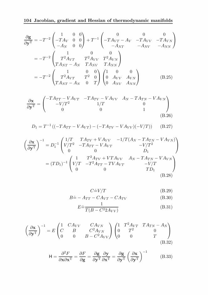
104 Jacobian, gradient and Hessian of thermodynamic manifolds
∂g
∂yT= −T−2
1 0 0−TAV 0 0−AN 0 0
+ T−1
0 0 0−TAV T −AV −TAV V −TAV N
−ANT −ANV −ANN
= −T−2
1 0 0T 2AV T T 2AV V T 2AV N
TANT −AN TANV TANN
= −T−2
1 0 0T 2AV T T 2 0
TANT −AN 0 T
1 0 00 AV V AV N
0 ANV ANN
(B.25)
∂x
∂yT=
−TATT − V AV T −TATV − V AV V AN − TATN − V AV N
−V/T 2 1/T 00 0 1
(B.26)
D1 = T−1 ((−TATT − V AV T )− (−TATV − V AV V )(−V/T )) (B.27)
(∂x
∂yT
)−1
= D−11
1/T TATV + V AV V −1/T (AN − TATN − V AV N )V/T 2 −TATT − V AV T −V/T 2
0 0 D1
= (TD1)−1
1 T 2ATV + V TAV V AN − TATN − V AV N
V/T −T 2ATT − TV AV T −V/T0 0 TD1
(B.28)
C=V/T (B.29)
B=−ATT − CAV T −CATV (B.30)
E=1
T (B − C22AV V )(B.31)
(∂x
∂yT
)−1
= E
1 CAV V CAV N
C B C2AV N
0 0 B − C2AV V
1 T 2AV T TATN −AN
0 T 2 00 0 T
(B.32)
H =∂2F
∂x∂xT=
∂F
∂g=
∂g
∂yT
∂y
∂xT=
∂g
∂yT
(∂x
∂yT
)−1
(B.33)
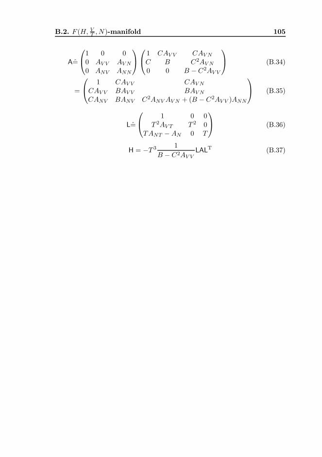
B.2. F (H, VT , N)-manifold 105
A=
1 0 00 AV V AV N
0 ANV ANN
1 CAV V CAV N
C B C2AV N
0 0 B −C2AV V
(B.34)
=
1 CAV V CAV N
CAV V BAV V BAV N
CANV BANV C2ANV AV N + (B − C2AV V )ANN
(B.35)
L=
1 0 0T 2AV T T 2 0
TANT −AN 0 T
(B.36)
H = −T 3 1
B − C2AV VLALT (B.37)


![arxiv.org · arXiv:0708.3981v2 [math.DG] 18 Apr 2008 GAPS IN THE DIFFERENTIAL FORMS SPECTRUM ON CYCLIC COVERINGS COLETTE ANNE, GILLES CARRON, AND OLAF POST´ Abstract. We are interested](https://static.fdocument.org/doc/165x107/606dd2e8423f9c26806a1dec/arxivorg-arxiv07083981v2-mathdg-18-apr-2008-gaps-in-the-differential-forms.jpg)