Numerical simulation of blood flow in LAD models with different
ENV5056 Numerical Modeling ofFlow and Contaminant Transport in Rivers
Numerical Solution of FlowEquationsEquations
Asst. Prof. Dr. Orhan GÜNDÜZ
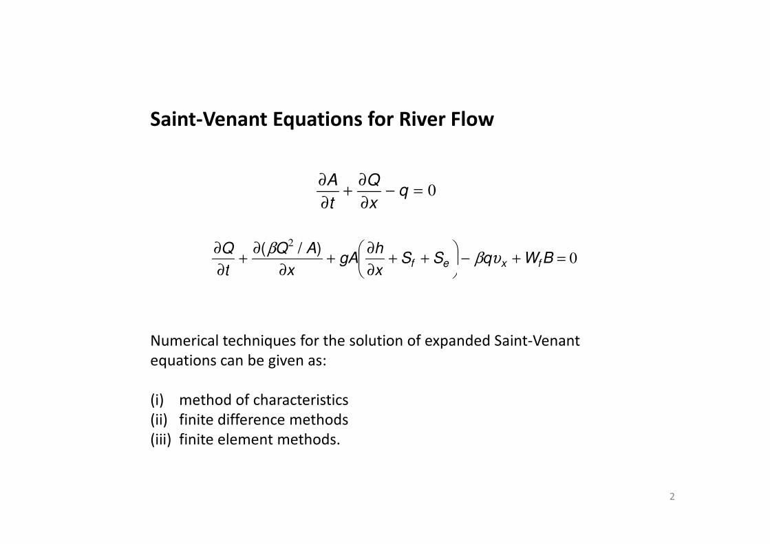
Saint-Venant Equations for River Flow
0=−∂
∂+
∂
∂q
x
Q
t
A
02
=+−
++
∂
∂+
∂
∂+
∂
∂BWqSS
x
hgA
x
AQ
t
Qfxef υβ
β )/(
2
∂∂∂ xxt
Numerical techniques for the solution of expanded Saint-Venantequations can be given as:
(i) method of characteristics(ii) finite difference methods(iii) finite element methods.
Of these methods, the finite element method is rarely used when flow is approximated as one-dimensional such as in the case of Saint-Venantequations. The other two methods have been commonly applied for the numerical solution of one-dimensional unsteady flow since 1960s.
The finite difference methods can further be classified as explicit and implicit techniques, each of which holds distinct numerical characteristics. A major advantage of the implicit finite difference method over the method of characteristic and the explicit finite difference technique is its inherent stability without the requirement to satisfy the Courant condition, which
3
stability without the requirement to satisfy the Courant condition, which sets the criteria for the maximum allowable time step. This requirement to satisfy Courant condition often makes the method of characteristics and explicit techniques very inefficient in terms of the use of computer time.
Furthermore, certain implicit schemes such as the Preissmann scheme (Preissmann, 1961) allow the use of variable time and spatial steps, which make them extremely convenient for applications in routing of flood hydrographs in river systems.
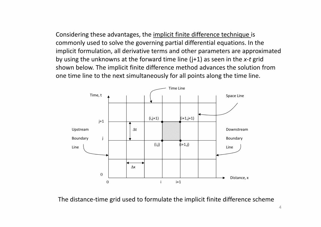
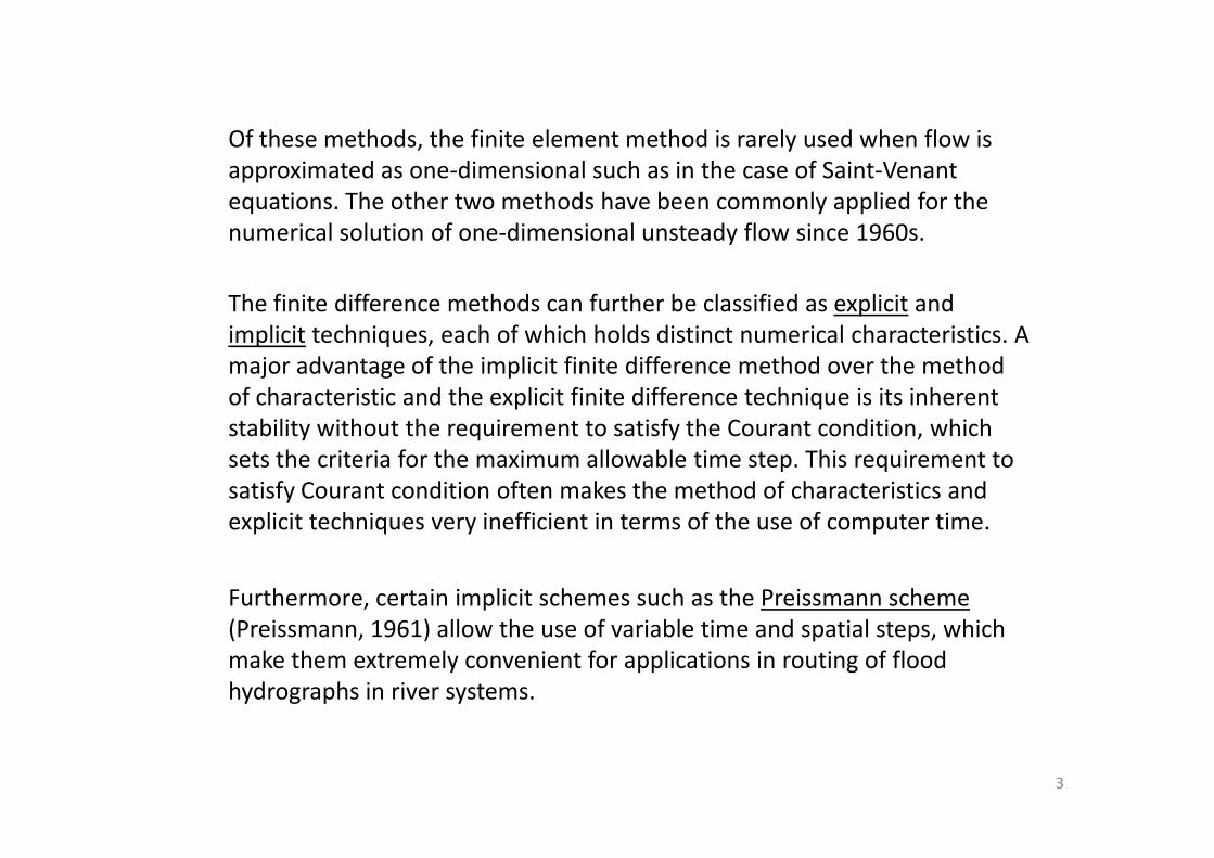
Considering these advantages, the implicit finite difference technique is commonly used to solve the governing partial differential equations. In the implicit formulation, all derivative terms and other parameters are approximated by using the unknowns at the forward time line (j+1) as seen in the x-t grid shown below. The implicit finite difference method advances the solution from one time line to the next simultaneously for all points along the time line.
Time Line
Space LineTime, t
4
∆x
∆t
(i,j) (i+1,j)
(i,j+1) (i+1,j+1)
0 i i+1
j
j+1
Distance, x0
Upstream
Boundary
Line
Downstream
Boundary
Line
The distance-time grid used to formulate the implicit finite difference scheme
Of the various implicit schemes that have been developed, the "weighted four-point" scheme first used by Preissmann (1961) is very advantageous since it can readily be used with unequal distance steps, which is particularly important for natural waterways where channel characteristics are highly variable even in short distances.
Similarly, the applicability of unequal time steps is another important characteristic of the Preissmann scheme, particularly in the case of
5
characteristic of the Preissmann scheme, particularly in the case of hydrograph routing where floodwaters would generally rise relatively quickly and recess gradually in time.
In this scheme, the four grid points from the (j)th and (j+1)th time lines are used to approximate the terms in the differential equation. A weighing factor,
θ, is used in the approximation of all terms of the equation except for the time derivatives in order to adjust the influence of the points (i) and (i+1).
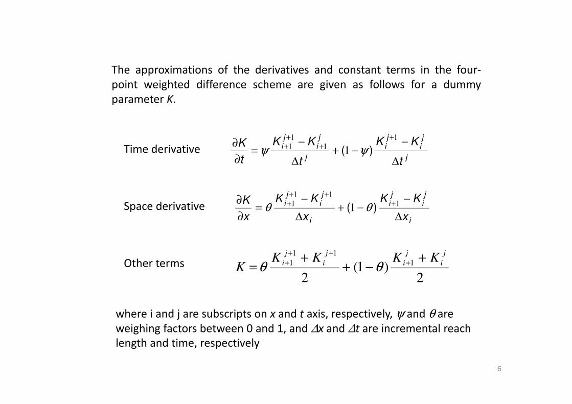
The approximations of the derivatives and constant terms in the four-point weighted difference scheme are given as follows for a dummyparameter K.
j
ji
ji
j
ji
ji
t
KK
t
KK
t
K
∆
−−+
∆
−=
∂
∂+
++
+1
11
1 1 )( ψψ
ji
ji
ji
ji KKKKK −
−+−
=∂ +
+++ 1
111 1 )( θθ
Time derivative
Space derivative
6
i
ii
i
ii
x
KK
x
KK
x
K
∆
−−+
∆
−=
∂
∂ ++ 11 1 )( θθ
2)1(
2
1
11
1
j
i
j
i
j
i
j
i KKKKK
+−+
+= +
+++ θθ
Space derivative
Other terms
where i and j are subscripts on x and t axis, respectively, ψ and θ are weighing factors between 0 and 1, and ∆x and ∆t are incremental reach length and time, respectively
It is possible to create different modifications of the implicit scheme for
various values of the weighing factors. Many researchers preferred using a ψvalue of 0.5 and approximated the time derivative at the center of grid
between (j)th and (j+1)th time lines On the other hand, different values of θwere used depending on the particular application.
If a θ value of 0.5 is used, the corresponding scheme is called the "box-scheme", which is a centered finite difference scheme. Similarly, a scheme
with a θ value of 1.0 is known as the "fully-implicit scheme" in space.
The weighted four-point implicit scheme is unconditionally stable for any
7
The weighted four-point implicit scheme is unconditionally stable for any
time step if the value of θ is selected between 0.5 and 1.0. In addition tostability criteria, analysis on the influence of the weighing factor on the
accuracy of computations revealed that the accuracy decreases as θ departsfrom 0.5 and approaches to 1.0. This effect became more pronounced as themagnitude of the computational time step increased. Furthermore, analysis
also revealed that a θ value of between 0.55 and 0.6 provided unconditionalstability and good accuracy, which makes this scheme superior compared tothe explicit scheme that requires time steps of less than a critical valuedetermined by the Courant condition.
Finite Difference Formulation with Preissmann Scheme
The finite difference equations of the Saint-Venant equations are discretizedin the x-t plane using the approximations given above. Two algebraic equations are obtained as a result of this approximation, representing the partial differential equations of continuity and momentum.
In the approximations given below, some of the variables are defined at the
8
In the approximations given below, some of the variables are defined at the nodes of the grid (i.e., Q, h, and A), whereas the others are defined for the
reach (i.e., Sf, Se, sc, sm and ∆x).
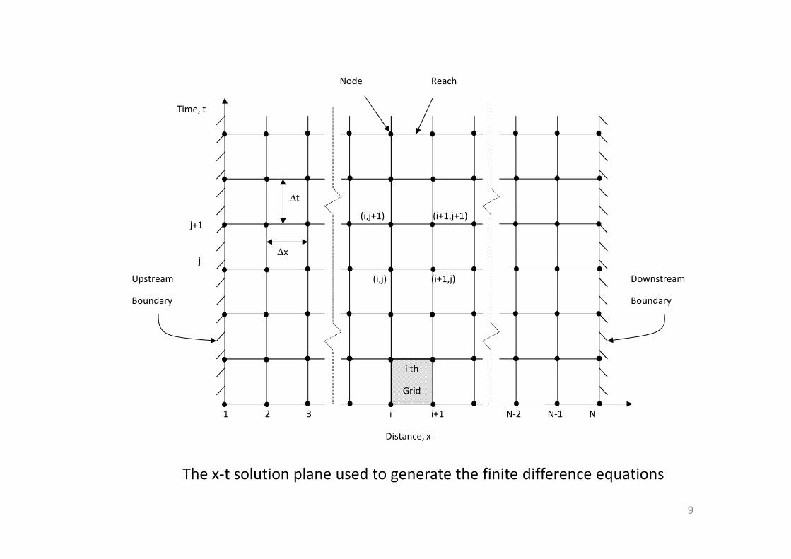
The variables defined for the reach are denoted by the subscript (i+½) in order to represent that these variables are defined half way between nodes (i) and (i+1), or on the reach. It is also seen that the solution plane is represented by a total of N nodes with node numbers starting from 1 and running through N.
(i,j) (i+1,j)
(i,j+1) (i+1,j+1)
j
j+1
Time, t
Upstream Downstream
∆x
∆t
Node Reach
9
i th
Grid
(i,j) (i+1,j)Upstream
Boundary
Downstream
Boundary
1 i i+1
Distance, x
2 3 NN-1N-2
The x-t solution plane used to generate the finite difference equations
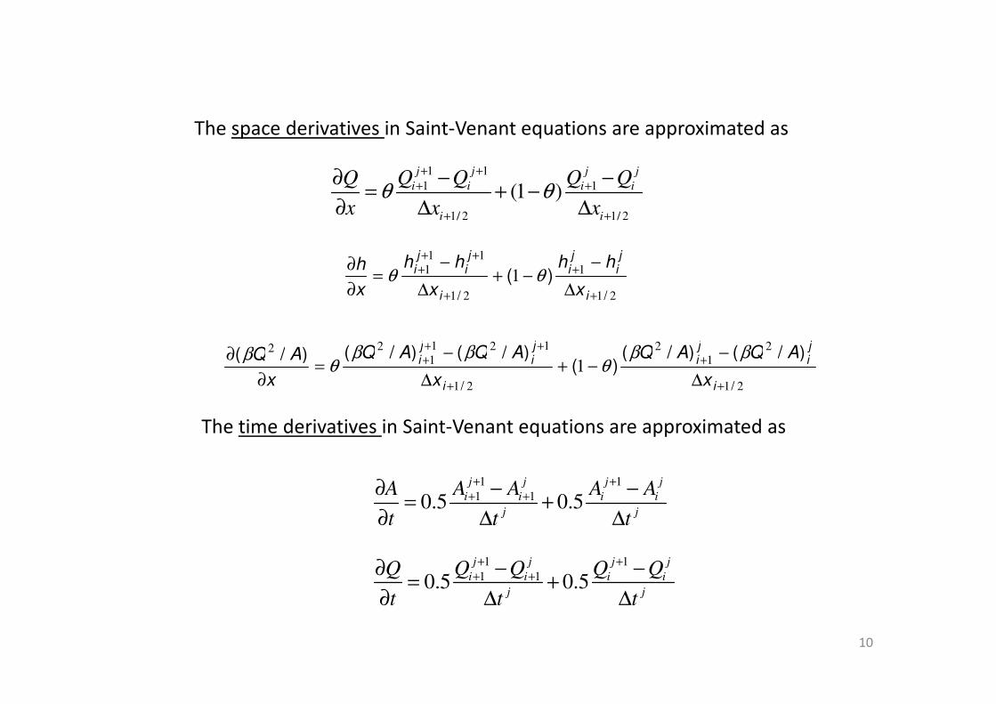
The space derivatives in Saint-Venant equations are approximated as
1 1
1 1
1/ 2 1/ 2
(1 )j j j j
i i i i
i i
Q Q Q QQ
x x xθ θ
+ ++ +
+ +
− −∂= + −
∂ ∆ ∆
21
1
21
11
1 1//
)(+
+
+
+++
∆
−−+
∆
−=
∂
∂
i
ji
ji
i
ji
ji
x
hh
x
hh
x
hθθ
2212122 )/()/()/()/()/( +++
+ −−∂jjjj AQAQAQAQAQ βββββ
10
21
21
2
21
121
122
1//
)/()/()(
)/()/()/(
+
+
+
+++
∆
−−+
∆
−=
∂
∂
i
ji
ji
i
ji
ji
x
AQAQ
x
AQAQ
x
AQ ββθ
ββθ
β
The time derivatives in Saint-Venant equations are approximated as
1 1
1 10.5 0.5j j j j
i i i i
j j
A A A AA
t t t
+ ++ +− −∂
= +∂ ∆ ∆
1 1
1 10.5 0.5j j j j
i i i i
j j
Q Q Q QQ
t t t
+ ++ +− −∂
= +∂ ∆ ∆
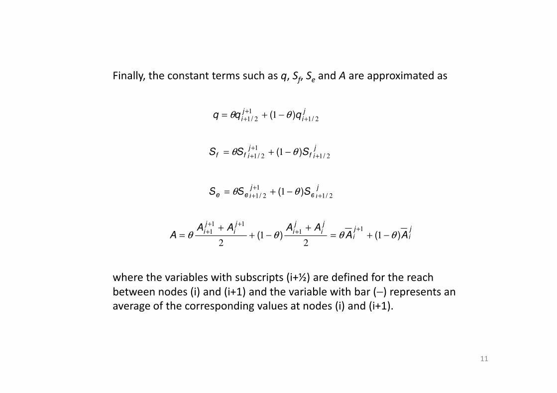
Finally, the constant terms such as q, Sf, Se and A are approximated as
ji
ji qqq
21
1
211 // )( +
++ −+= θθ
jif
jiff SSS
21
1
211 // )( +
++ −+= θθ
j
iej
iee SSS21
1
211
//)( +
++ −+= θθ
11
ieiee SSS2121
1//
)( ++ −+= θθ
ji
ji
ji
ji
ji
ji AA
AAAAA )()( θθθθ −+=
+−+
+=
++++
+ 12
12
1111
1
where the variables with subscripts (i+½) are defined for the reach
between nodes (i) and (i+1) and the variable with bar (−) represents an average of the corresponding values at nodes (i) and (i+1).
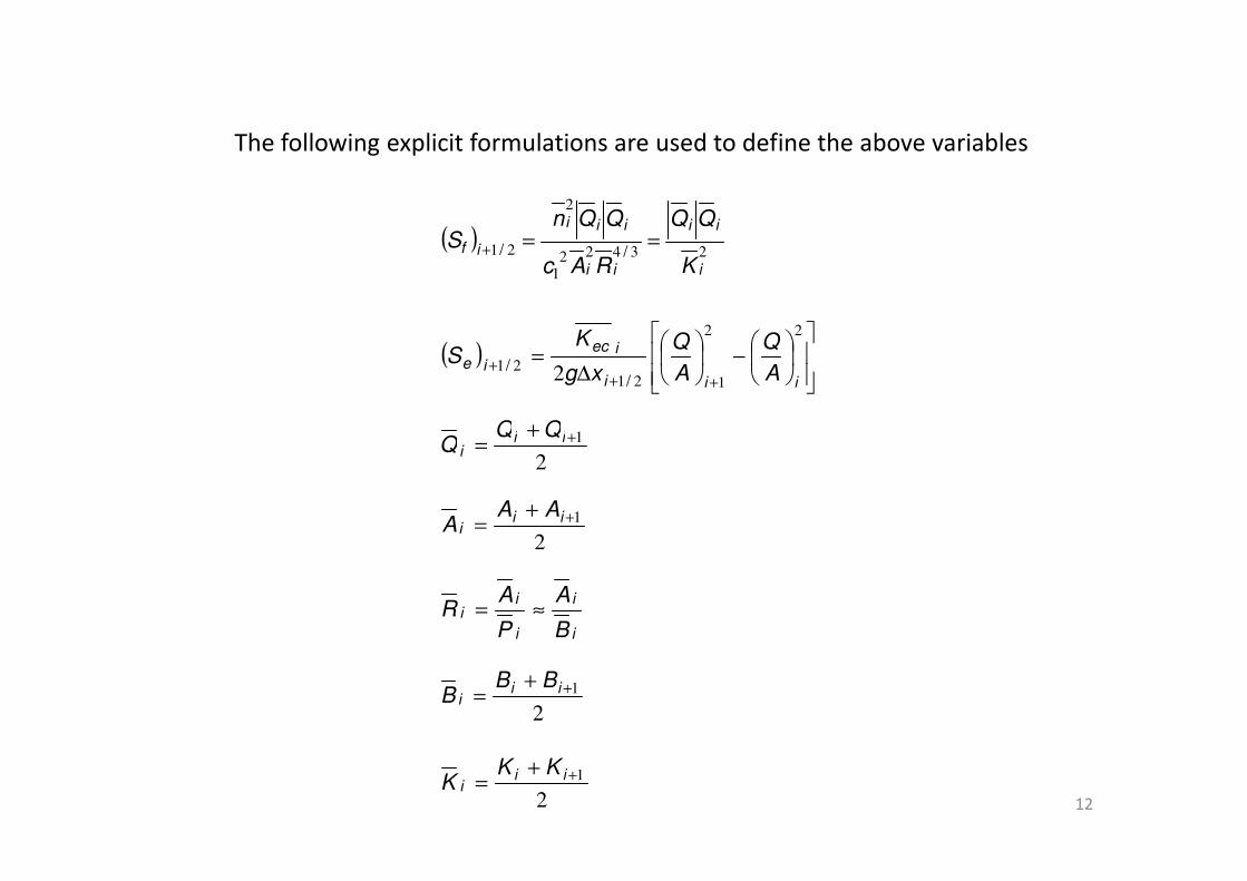
The following explicit formulations are used to define the above variables
( )23422
1
2
21
i
ii
ii
iii
if
K
RAc
QQnS ==+ //
( )
−
∆=
+++
22
12121 2 iii
iec
ieA
Q
A
Q
xg
KS
//
1++= ii QQ
Q
12
2
1++= ii
i
QQQ
2
1++= ii
iAA
A
i
i
i
ii
B
A
P
AR ≈=
2
1++= ii
iBB
B
2
1++= ii
iKK
K
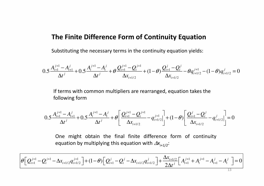
The Finite Difference Form of Continuity Equation
Substituting the necessary terms in the continuity equation yields:
1 1 1 111 1 1 1
1/ 2 1/ 2
1/ 2 1/ 2
0.5 0.5 (1 ) (1 ) 0j j j j j j j j
j ji i i i i i i ii ij j
i i
A A A A Q Q Q Qq q
t t x xθ θ θ θ
+ + + +++ + + +
+ +
+ +
− − − −+ + + − − − − =
∆ ∆ ∆ ∆
If terms with common multipliers are rearranged, equation takes the
13
If terms with common multipliers are rearranged, equation takes the following form
1 1 1 111 1 1 1
1/ 2 1/ 2
1/ 2 1/ 2
0.5 0.5 (1 ) 0j j j j j j j j
j ji i i i i i i ii ij j
i i
A A A A Q Q Q Qq q
t t x xθ θ
+ + + +++ + + +
+ +
+ +
− − − −+ + − + − − =
∆ ∆ ∆ ∆
One might obtain the final finite difference form of continuity
equation by multiplying this equation with ∆xi+1/2:
1 1 1 1 11/ 21 1/ 2 1/ 2 1 1/ 2 1/ 2 1 1(1 ) 0
2
j j j j j j j j j jii i i i i i i i i i i ij
xQ Q x q Q Q x q A A A A
tθ θ+ + + + ++
+ + + + + + + +
∆ − − ∆ + − − − ∆ + + − − = ∆
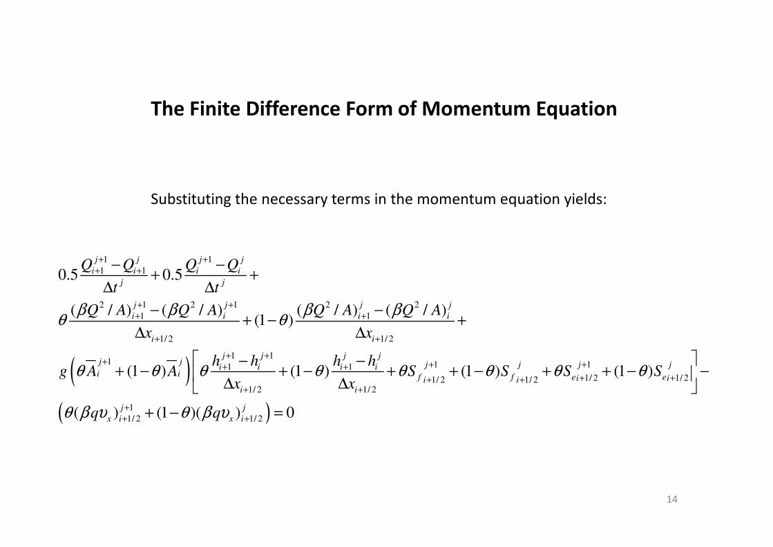
The Finite Difference Form of Momentum Equation
Substituting the necessary terms in the momentum equation yields:
1 1
1 10.5 0.5j j j j
i i i iQ Q Q Q+ +
+ +− −+ +
14
( )
1 1
2 1 2 1 2 2
1 1
1/ 2 1/ 2
1 11 11 1
1/ 21/ 2 1/ 21/ 2 1/ 2
0.5 0.5
( / ) ( / ) ( / ) ( / )(1 )
(1 ) (1 ) (1 )
i i i i
j j
j j j j
i i i i
i i
j j j jj j j j ji i i ii i f f eii i
i i
t t
Q A Q A Q A Q A
x x
h h h hg A A S S S
x x
β β β βθ θ
θ θ θ θ θ θ θ
+ +
+ ++ +
+ +
+ ++ + ++ +
++ ++ +
+ +∆ ∆
− −+ − +
∆ ∆
− −+ − + − + + − +
∆ ∆
( )
1
1/ 2
1
1/ 2 1/ 2
(1 )
( ) (1 )( ) 0
j
ei
j j
x i x i
S
q q
θ
θ β υ θ β υ
+
++ +
+ − −
+ − =
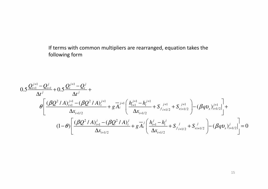
If terms with common multipliers are rearranged, equation takes the following form
1 1
1 10.5 0.5j j j j
i i i i
j j
Q Q Q Q
t t
+ ++ +− −
+ +∆ ∆
15
2 1 2 1 1 11 1 1 11 1
1/ 21/ 21/ 21/ 2 1/ 2
2
1
( / ) ( / ) ( )
( / ) (1 )
j j j jj j j ji i i ii f e x iii
i i
j
i
t t
Q A Q A h hg A S S q
x x
Q A
β βθ β υ
βθ
+ + + ++ + + ++ +
++++ +
+
∆ ∆
− −+ + + − +
∆ ∆
−2
11/ 21/ 21/ 2
1/ 2 1/ 2
( / )( ) 0
j j jj j j ji i ii f e x iii
i i
Q A h hg A S S q
x x
ββ υ+
++++ +
− −+ + + − =
∆ ∆
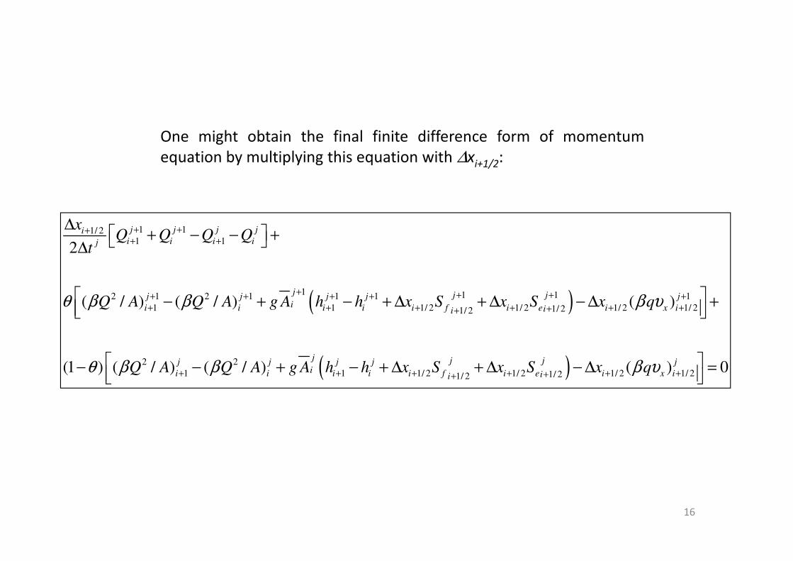
One might obtain the final finite difference form of momentum
equation by multiplying this equation with ∆xi+1/2:
( )
1 11/ 21 1
2
j j j jii i i ij
xQ Q Q Q
t
+ +++ +
∆ + − − + ∆
16
( )1 1 12 1 2 1 1 1 1
1 1 1/ 2 1/ 2 1/ 2 1/ 21/ 21/ 2
2 2
1 1 1/ 2
( / ) ( / ) ( )
(1 ) ( / ) ( / )
j j jj j j j jii i i i i f i e i x iii
jj j j j
ii i i i i f
Q A Q A g A h h x S x S x q
Q A Q A g A h h x S
θ β β β υ
θ β β
+ + ++ + + + ++ + + + + +++
+ + +
− + − + ∆ + ∆ − ∆ +
− − + − + ∆( )1/ 2 1/ 2 1/ 21/ 21/ 2( ) 0
j j j
i e i x iiix S x qβ υ+ + +++
+ ∆ − ∆ =
The terms with subscript (j) in continuity and momentum equations are known either from initial conditions or from the solution of Saint-Venantequations at the previous time line.
Since cross sectional area (A) and channel top width (B) are functions of water surface elevation (h), the only unknown terms in these equations are discharge (Q) and water surface elevation (h) at the (j+1)th time line at nodes (i) and (i+1).
17
Therefore, there are only four unknowns in these equations. All remaining terms are either constants or are functions of these unknowns. The finite difference forms of continuity and momentum equations are solved for each grid shown before.
The resulting two algebraic equations obtained by the application of the
weighted four-point scheme are nonlinear and an iterative solution
technique is required.
As there are N-1 grids in a time line, a total of 2*(N-1) equations are formed for one time line between the upstream and downstream boundary.
There are two unknowns (Q and h) in each of the N nodes giving a total of 2N unknown along each time line. The system of 2(N-1) equations with 2N unknown require two additional equations to be determinate.
18
These two additional equations are supplied by the upstream and downstream boundary conditions.
The resulting system of 2N non-linear equations with 2N unknowns is commonly solved by the Newton-Raphson iterative technique to handle the non-linearity in the equations.
The Boundary Conditions
The two additional equations required for the system to be determinate come from the external boundaries at the upstream and downstream locales of the reach. Two types of boundary conditions can be specified at the upstream boundary:
1. Discharge Hydrograph2. Stage (or Depth) Hydrograph
19
2. Stage (or Depth) Hydrograph
At the downstream boundary, it is possible to specify one of the five available conditions given as:
1. Discharge Hydrograph2. Stage (or Depth) Hydrograph3. Single-Valued Rating Curve4. Looped Rating Curve5. Critical Flow Section
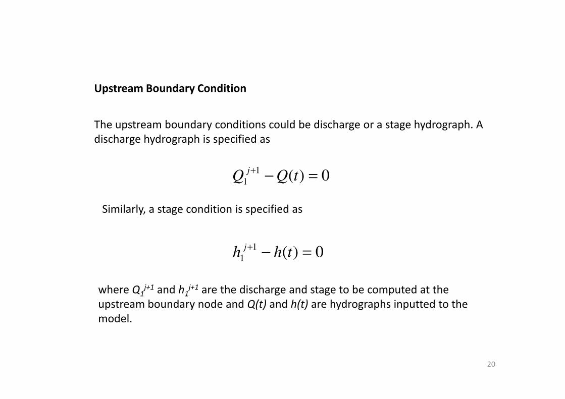
Upstream Boundary Condition
The upstream boundary conditions could be discharge or a stage hydrograph. A discharge hydrograph is specified as
0)( 1
1 =−+tQQ
j
20
Similarly, a stage condition is specified as
0)(1
1 =−+thh
j
where Q1j+1 and h1
j+1 are the discharge and stage to be computed at the upstream boundary node and Q(t) and h(t) are hydrographs inputted to the model.
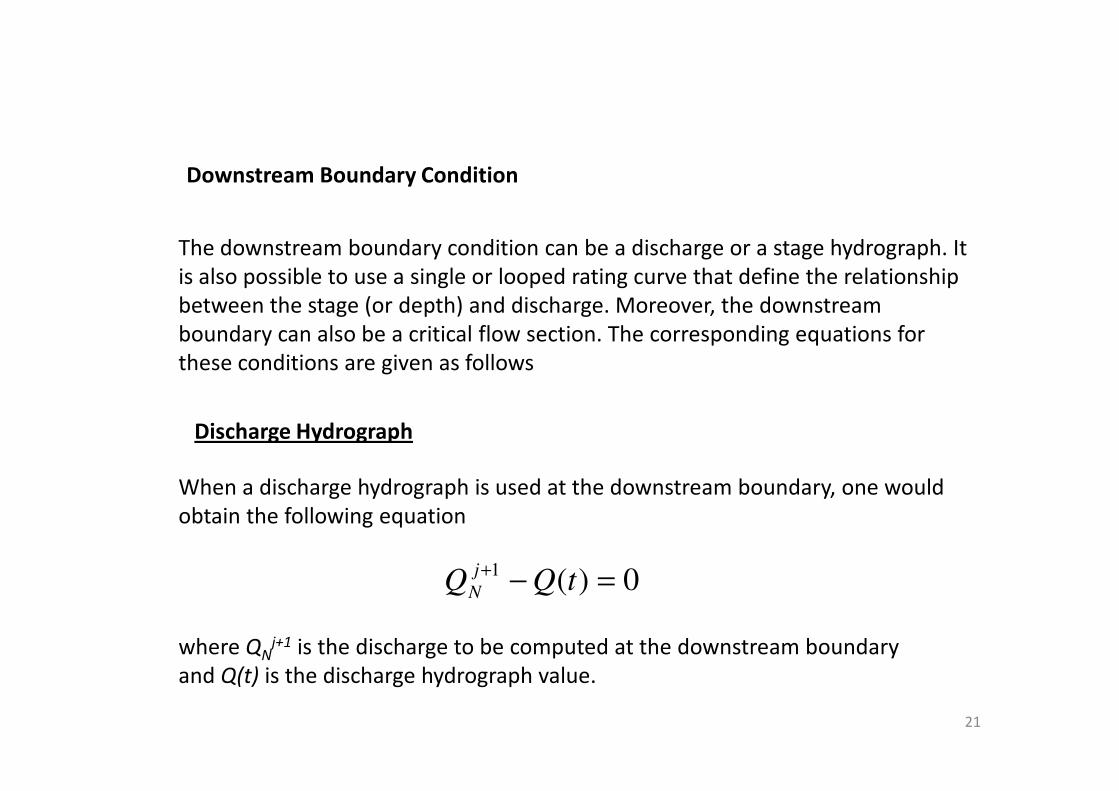
Downstream Boundary Condition
The downstream boundary condition can be a discharge or a stage hydrograph. It is also possible to use a single or looped rating curve that define the relationship between the stage (or depth) and discharge. Moreover, the downstream boundary can also be a critical flow section. The corresponding equations for these conditions are given as follows
21
Discharge Hydrograph
When a discharge hydrograph is used at the downstream boundary, one would obtain the following equation
0)( 1 =−+tQQ
j
N
where QNj+1 is the discharge to be computed at the downstream boundary
and Q(t) is the discharge hydrograph value.
Improper use of a discharge hydrograph at the downstream boundary can result in gross errors. The imposed flow may exceed the capacity of the channel to deliver water to that node. Moreover, if a discharge condition is also specified at the upstream boundary, any error in the values of these flows is reflected in the water levels which might sometimes cause the stream be partially or completely dry. In this regard, a discharge condition at the downstream boundary is rarely used in unsteady flow simulations
22
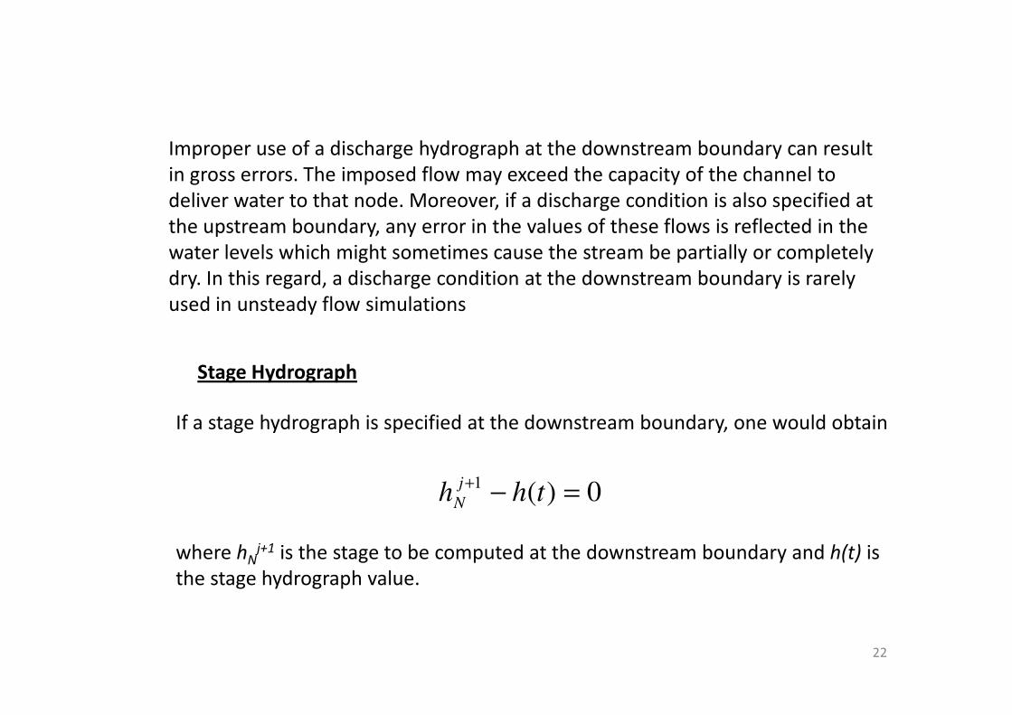
Stage Hydrograph
If a stage hydrograph is specified at the downstream boundary, one would obtain
0)( 1 =−+thh
j
N
where hNj+1 is the stage to be computed at the downstream boundary and h(t) is
the stage hydrograph value.
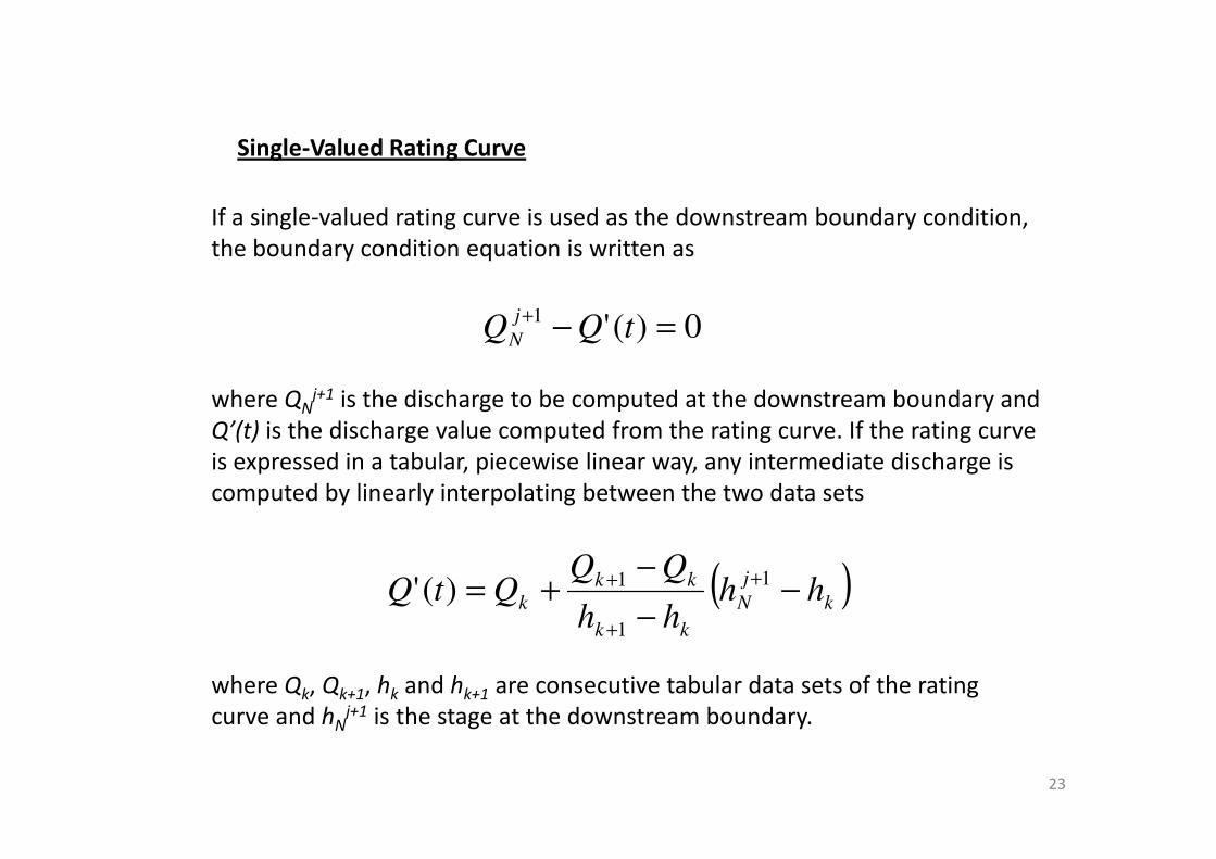
Single-Valued Rating Curve
If a single-valued rating curve is used as the downstream boundary condition, the boundary condition equation is written as
0)(' 1 =−+tQQ
j
N
where QNj+1 is the discharge to be computed at the downstream boundary and
Q’(t) is the discharge value computed from the rating curve. If the rating curve
23
Q’(t) is the discharge value computed from the rating curve. If the rating curve is expressed in a tabular, piecewise linear way, any intermediate discharge is computed by linearly interpolating between the two data sets
( )k
j
N
kk
kk
k hhhh
QQQtQ −
−
−+= +
+
+ 1
1
1)('
where Qk, Qk+1, hk and hk+1 are consecutive tabular data sets of the rating curve and hN
j+1 is the stage at the downstream boundary.
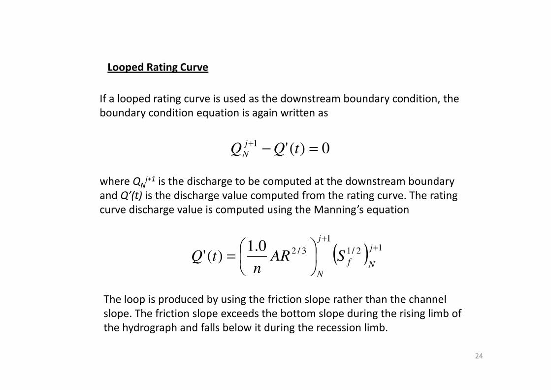
Looped Rating Curve
If a looped rating curve is used as the downstream boundary condition, the boundary condition equation is again written as
0)(' 1 =−+tQQ
j
N
where QNj+1 is the discharge to be computed at the downstream boundary
and Q’(t) is the discharge value computed from the rating curve. The rating
24
and Q’(t) is the discharge value computed from the rating curve. The rating curve discharge value is computed using the Manning’s equation
( ) 12/1
1
3/20.1)('
++
=
j
Nf
j
N
SARn
tQ
The loop is produced by using the friction slope rather than the channel slope. The friction slope exceeds the bottom slope during the rising limb of the hydrograph and falls below it during the recession limb.
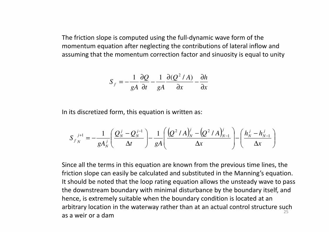
The friction slope is computed using the full-dynamic wave form of the momentum equation after neglecting the contributions of lateral inflow and assuming that the momentum correction factor and sinuosity is equal to unity
x
h
x
AQ
gAt
Q
gAS f
∂
∂−
∂
∂−
∂
∂−=
)/(11 2
In its discretized form, this equation is written as:
25
( ) ( )
∆
−−
∆
−−
∆
−−= −−
−+
x
hh
x
AQAQ
gAt
gAS
j
N
j
N
j
N
j
N
j
N
j
N
j
N
j
Nf
11
2211 //11
Since all the terms in this equation are known from the previous time lines, the friction slope can easily be calculated and substituted in the Manning’s equation. It should be noted that the loop rating equation allows the unsteady wave to pass the downstream boundary with minimal disturbance by the boundary itself, and hence, is extremely suitable when the boundary condition is located at an arbitrary location in the waterway rather than at an actual control structure such as a weir or a dam
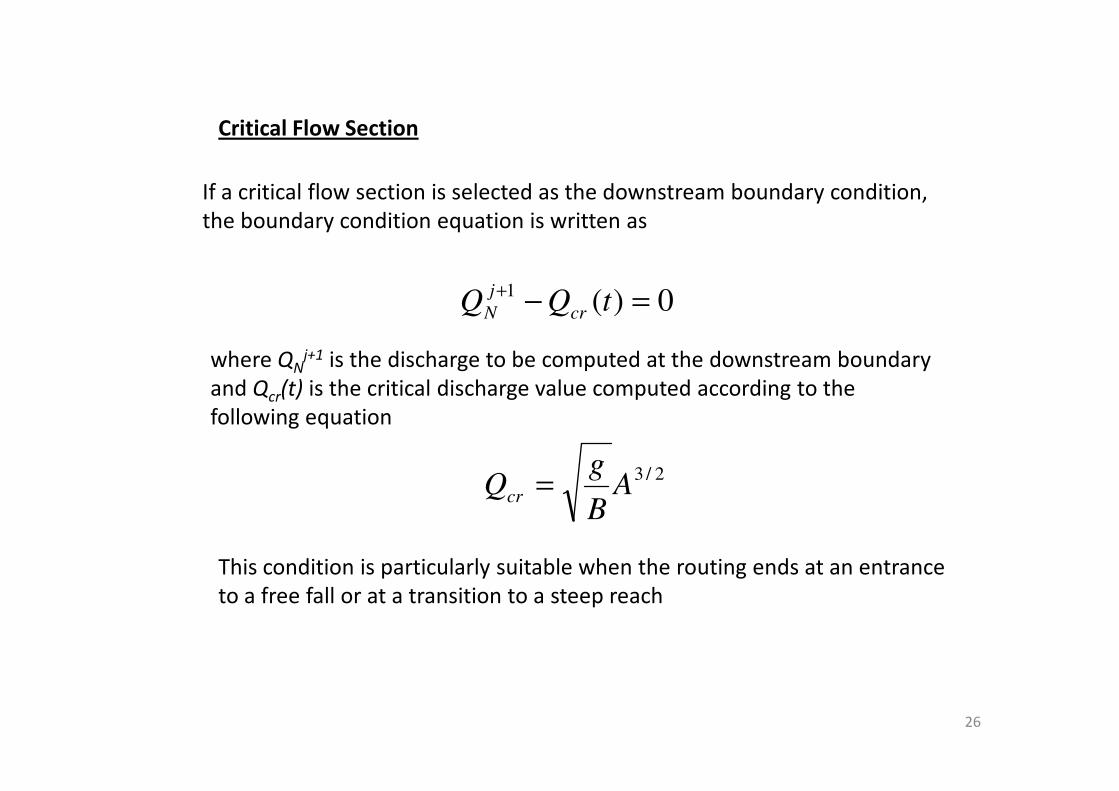
Critical Flow Section
If a critical flow section is selected as the downstream boundary condition, the boundary condition equation is written as
0)( 1 =−+tQQ cr
j
N
where QNj+1 is the discharge to be computed at the downstream boundary
and Qcr(t) is the critical discharge value computed according to the
26
and Qcr(t) is the critical discharge value computed according to the following equation
2/3A
B
gQcr =
This condition is particularly suitable when the routing ends at an entrance to a free fall or at a transition to a steep reach
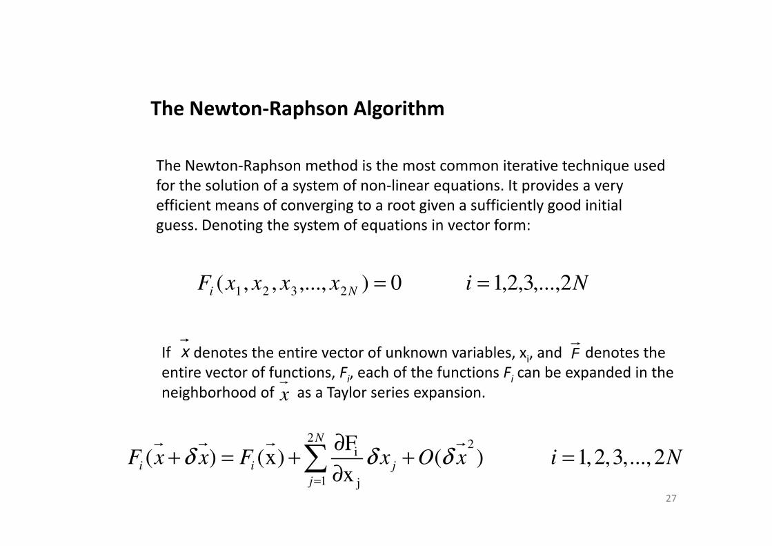
The Newton-Raphson Algorithm
The Newton-Raphson method is the most common iterative technique used for the solution of a system of non-linear equations. It provides a very efficient means of converging to a root given a sufficiently good initial guess. Denoting the system of equations in vector form:
NixxxxF 2,...,3,2,1 0),...,,,( ==
27
NixxxxF Ni 2,...,3,2,1 0),...,,,( 2321 ==
x F
x�
If denotes the entire vector of unknown variables, xi, and denotes the entire vector of functions, Fi, each of the functions Fi can be expanded in the
neighborhood of as a Taylor series expansion.
22
i
1 j
F( ) (x) ( ) 1, 2,3,..., 2
x
N
i i j
j
F x x F x O x i Nδ δ δ=
∂+ = + + =
∂∑
� � � �
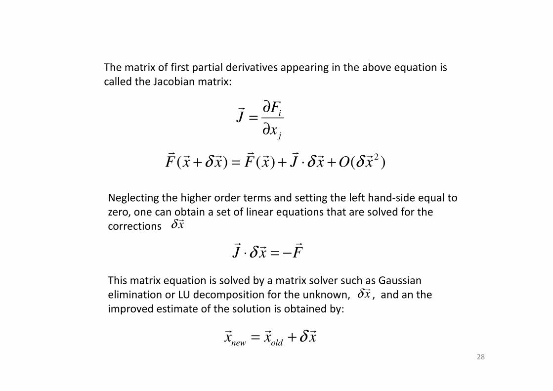
The matrix of first partial derivatives appearing in the above equation is called the Jacobian matrix:
i
j
FJ
x
∂=
∂
�
2( ) ( ) ( )F x x F x J x O xδ δ δ+ = + ⋅ +� � �
� � � � �
Neglecting the higher order terms and setting the left hand-side equal to
28
Neglecting the higher order terms and setting the left hand-side equal to zero, one can obtain a set of linear equations that are solved for the corrections xδ
�
J x Fδ⋅ = −� �
�
This matrix equation is solved by a matrix solver such as Gaussian elimination or LU decomposition for the unknown, , and an the improved estimate of the solution is obtained by:
xδ�
new oldx x xδ= +� � �
The iteration process is continued until a predetermined convergence level is achieved. It is important to assign different convergence criteria for Q and h values. A generally accepted convergence criteria for h is 0.01 ft or 3 mm (Fread, 1985). The convergence criteria for Q is computed according to the following equality:
BVhQ εε =
where εQ and εh are convergence criteria for discharge and water surfaceelevation, respectively; B is the top width of the cross section and V is the
29
elevation, respectively; B is the top width of the cross section and V is theflow velocity.
The convergence process depends on a good first estimate for the unknownvariables. A reasonably good estimate for the first time step is to use theinitial condition of discharge (Q) and water surface elevation (h). For anyother time step, the first estimates of the unknown variables can be obtainedby using the linearly extrapolated values from solutions at previous timesteps.
Partial Derivatives of Finite Difference Equations
One of the discouraging issues about the Newton-Raphson technique is the need to evaluate the partial derivative terms of the Jacobian matrix. When the equations get complex, it might get very difficult to differentiate the difference equations. However, it is this feature of the technique that provides fast convergence to the root.
In this regard, the difference forms of continuity and momentum equations are
30
In this regard, the difference forms of continuity and momentum equations are partially differentiated with respect to the unknown terms h and Q at the (j+1)th
time line for the reaches (i) and (i+1).
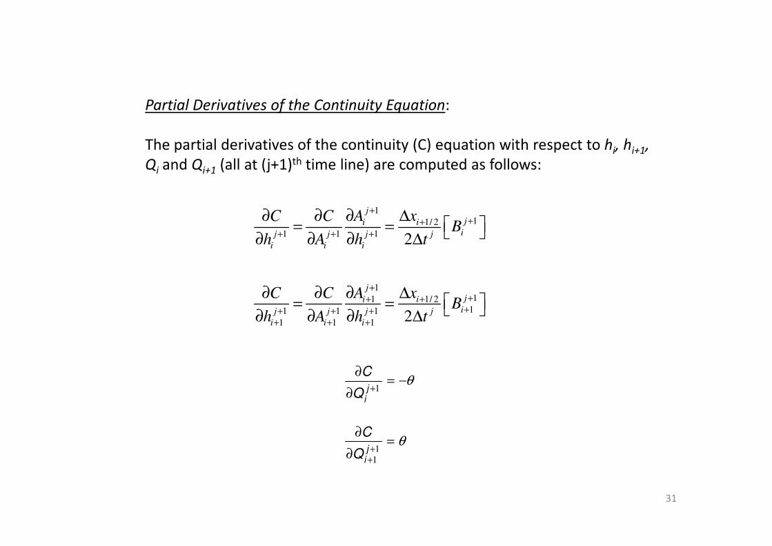
Partial Derivatives of the Continuity Equation:
The partial derivatives of the continuity (C) equation with respect to hi, hi+1,
Qi and Qi+1 (all at (j+1)th time line) are computed as follows:
111/ 2
1 1 1 2
jji i
ij j j j
i i i
A xC CB
h A h t
+++
+ + +
∂ ∆∂ ∂ = = ∂ ∂ ∂ ∆
31
111 1/ 2
11 1 1
1 1 1 2
jji i
ij j j j
i i i
A xC CB
h A h t
+++ +
++ + ++ + +
∂ ∆∂ ∂ = = ∂ ∂ ∂ ∆
θ−=∂
∂+1j
iQ
C
θ=∂
∂+
+1
1jiQ
C
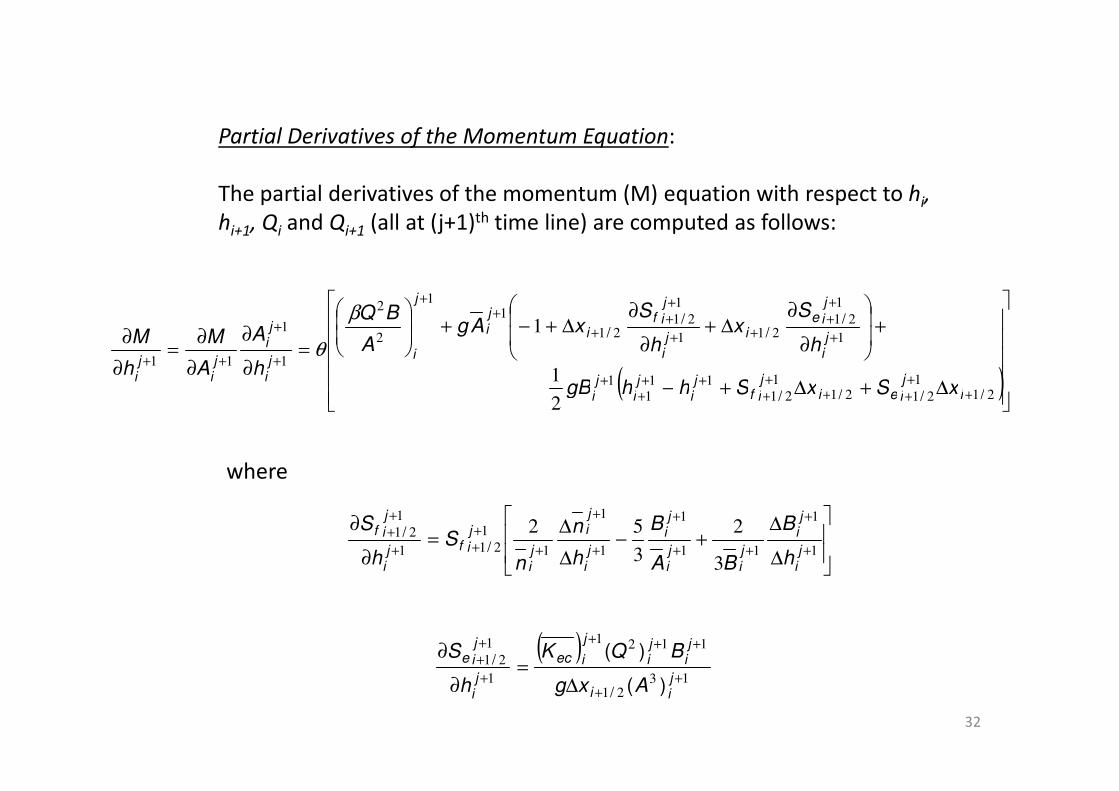
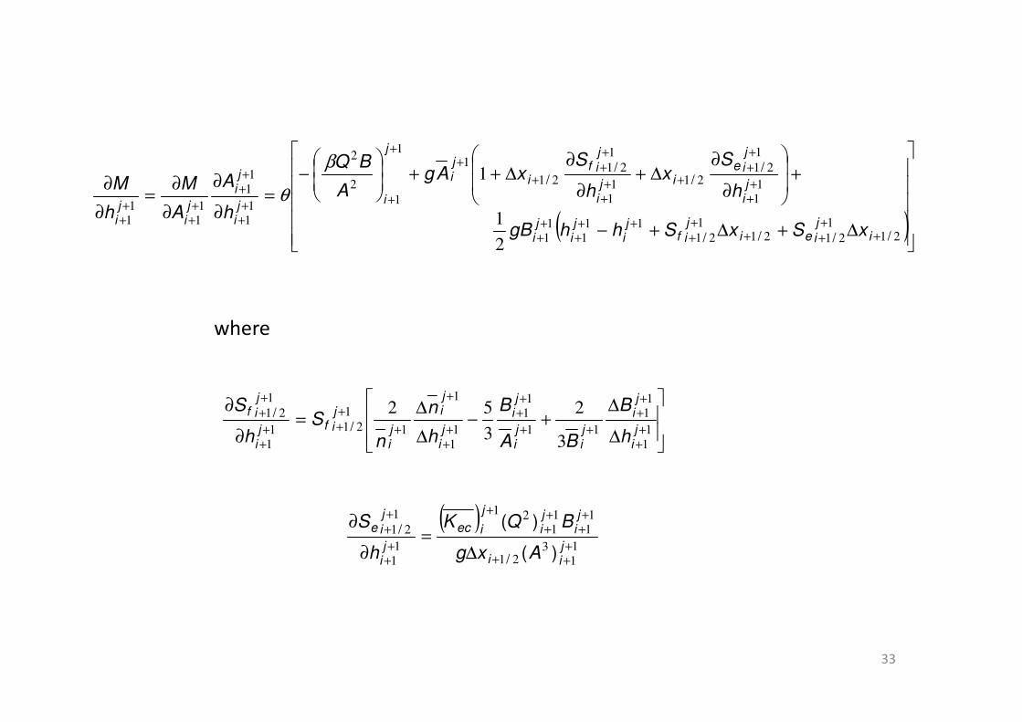
Partial Derivatives of the Momentum Equation:
The partial derivatives of the momentum (M) equation with respect to hi,
hi+1, Qi and Qi+1 (all at (j+1)th time line) are computed as follows:
( )
∆+∆+−
+
∂
∂∆+
∂
∂∆+−+
=∂
∂
∂
∂=
∂
∂
++++
++
+++
+
+
++
++
++
+
++
+
+
++
211
21211
2111
11
1
1
21211
1
2121
11
2
2
1
1
11
2
1
1
////
//
//
ij
ieijif
ji
ji
ji
ji
j
ieij
i
jif
i
ji
j
iji
ji
ji
ji
xSxShhgB
h
Sx
h
SxAg
A
BQ
h
A
A
M
h
M
β
θ
32
( )∆+∆+− +++++ 212121211
2//// iieiifiii xSxShhgB
∆
∆+−
∆
∆=
∂
∂
+
+
++
+
+
+
+
+++
++
1
1
11
1
1
1
1
1
211
1
21
3
2
3
52ji
ji
ji
ji
ji
ji
ji
ji
jifj
i
jif
h
B
BA
B
h
n
n
Sh
S/
/
where
( )13
21
1121
1
1
21
++
+++
+
++
∆=
∂
∂
jii
ji
ji
j
iec
ji
j
ie
Axg
BQK
h
S
)(
)(
/
/
( )
∆+∆+−
+
∂
∂∆+
∂
∂∆++
−
=∂
∂
∂
∂=
∂
∂
++++
++
+++
++
++
++
+++
++
+
++
+++
++
++
++
211
21211
2111
11
1
11
1
21211
1
1
2121
11
1
2
2
11
1
1
11
11
2
1
1
////
//
//
ij
ieijif
ji
ji
ji
ji
j
ieij
i
jif
i
ji
j
iji
ji
ji
ji
xSxShhgB
h
Sx
h
SxAg
A
BQ
h
A
A
M
h
M
β
θ
where
33
∆
∆+−
∆
∆=
∂
∂
++
++
++
++
++
+
+
+++
+
++
1
1
11
11
11
1
1
1
1
1
211
1
1
21
3
2
3
52ji
ji
ji
ji
ji
ji
ji
ji
jifj
i
jif
h
B
BA
B
h
n
n
Sh
S/
/
( )11
321
11
11
21
11
1
21
+++
++
++
+
++
++
∆=
∂
∂
jii
ji
ji
j
iec
ji
j
ie
Axg
BQK
h
S
)(
)(
/
/
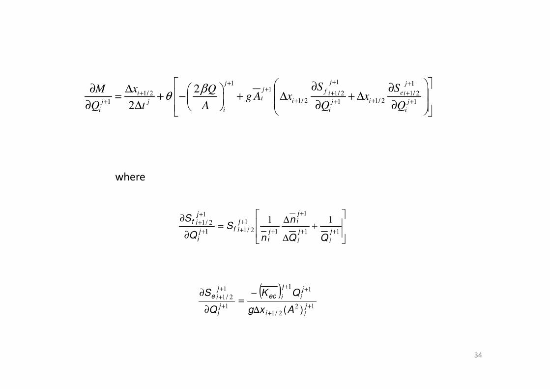
11 11
1/ 2 1/ 2 1/ 21/ 2 1/ 21 1 1
2
2
jj jj f ei i ii i ij j j j
ii i i
S SxM Qg A x x
Q t A Q Q
βθ
++ ++
+ + ++ ++ + +
∂ ∂∆∂ = + − + ∆ + ∆ ∂ ∆ ∂ ∂
where
34
+
∆
∆=
∂
∂
++
+
+
+++
++
11
1
1
1
211
1
21 11j
i
j
i
ji
ji
jifj
i
jif
n
n
SQ
S/
/
( )12
21
11
1
1
21
++
++
+
++
∆
−=
∂
∂
jii
ji
j
iec
ji
j
ie
Axg
QK
Q
S
)(/
/
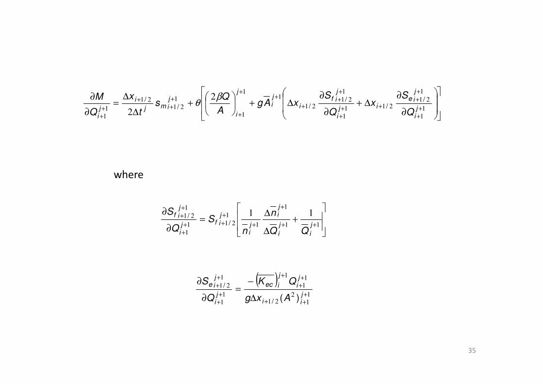
∂
∂∆+
∂
∂∆+
+
∆
∆=
∂
∂+
+
++
+++
++
+
++
+
++
+
++
1
1
1
21211
1
1
2121
11
1
1
2121
1
1
2
2ji
j
ieij
i
jif
i
ji
j
i
jimj
i
ji Q
Sx
Q
SxAg
A
Qs
t
x
Q
M //
///
/ βθ
where
35
+
∆
∆=
∂
∂
++
+
+
+++
+
++
11
1
1
1
211
1
1
21 11j
i
j
i
ji
ji
jifj
i
jif
n
n
SQ
S/
/
( )11
221
11
1
11
1
21
+++
++
+
++
++
∆
−=
∂
∂
jii
ji
j
iec
ji
j
ie
Axg
QK
Q
S
)(/
/
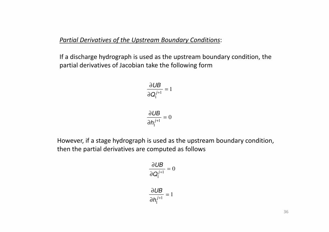
Partial Derivatives of the Upstream Boundary Conditions:
If a discharge hydrograph is used as the upstream boundary condition, the partial derivatives of Jacobian take the following form
11
1
=∂
∂+jQ
UB
0=∂UB
36
01
1
=∂
∂+jh
UB
However, if a stage hydrograph is used as the upstream boundary condition, then the partial derivatives are computed as follows
01
1
=∂
∂+jQ
UB
11
1
=∂
∂+jh
UB
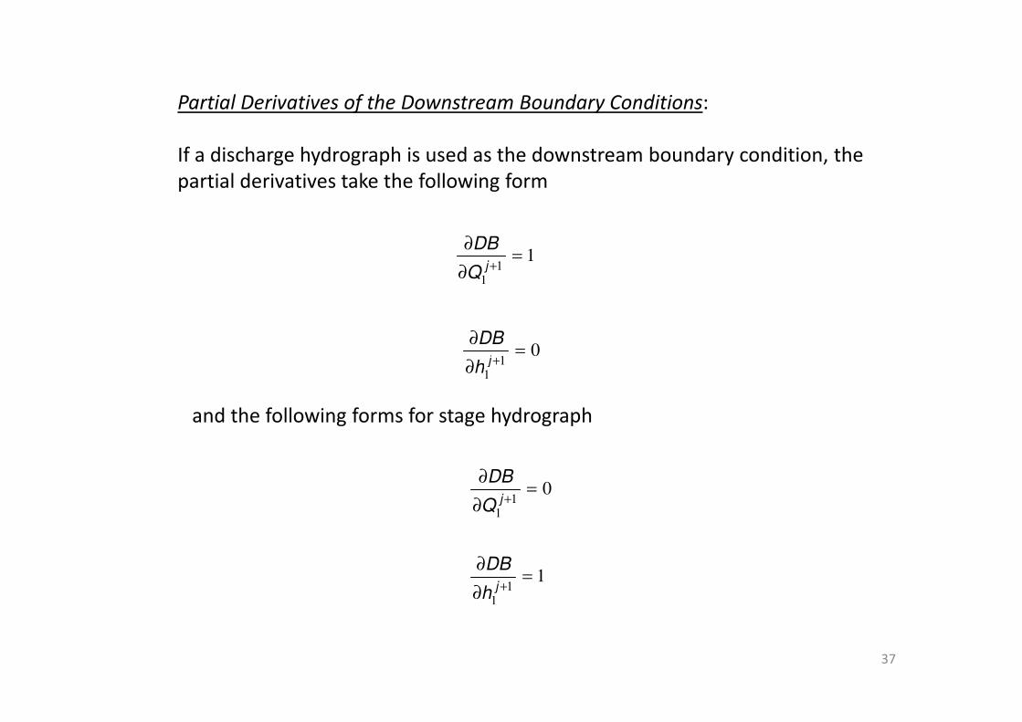
Partial Derivatives of the Downstream Boundary Conditions:
If a discharge hydrograph is used as the downstream boundary condition, the partial derivatives take the following form
11
1
=∂
∂+jQ
DB
01
=∂
∂+jh
DB
37
11∂ +jh
and the following forms for stage hydrograph
01
1
=∂
∂+jQ
DB
11
1
=∂
∂+jh
DB
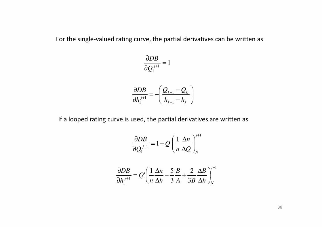
For the single-valued rating curve, the partial derivatives can be written as
11
1
=∂
∂+j
Q
DB
−
−−=
∂
∂
+
+
+kk
kk
j hh
h
DB
1
1
1
1
38
If a looped rating curve is used, the partial derivatives are written as
1
1
1
1'1
+
+
∆
∆+=
∂
∂j
N
j Q
n
nQ
Q
DB
1
1
13
2
3
51'
+
+
∆
∆+−
∆
∆=
∂
∂j
N
j h
B
BA
B
h
n
nQ
h
DB
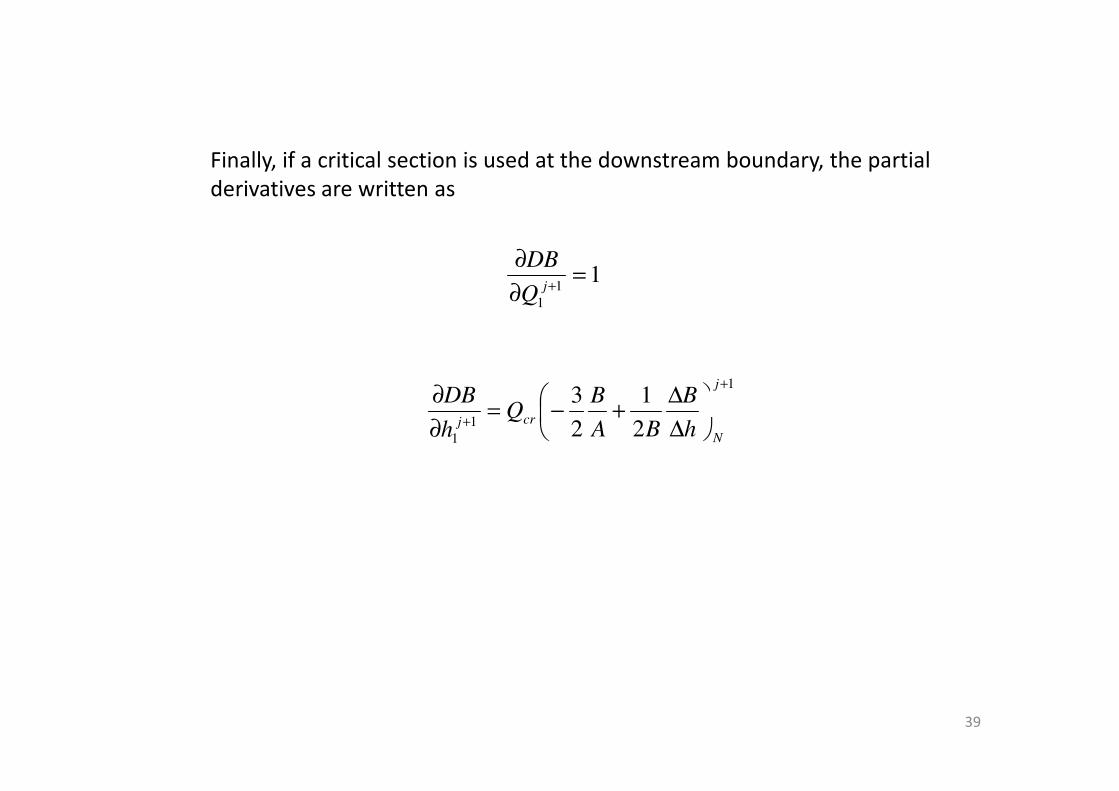
Finally, if a critical section is used at the downstream boundary, the partial derivatives are written as
11
1
=∂
∂+j
Q
DB
113
+
∆
+−=∂
jBBDB
39
1
12
1
2
3+
∆
∆+−=
∂
∂
N
crj h
B
BA
BQ
h
DB
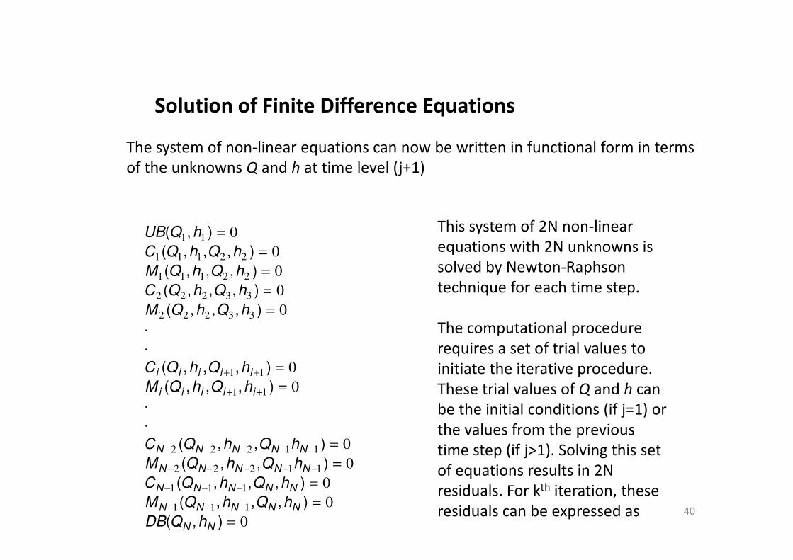
Solution of Finite Difference Equations
The system of non-linear equations can now be written in functional form in terms of the unknowns Q and h at time level (j+1)
0
0
0
22111
22111
11
=
=
=
=
),,,(
),,,(
),(
hQhQM
hQhQC
hQUB This system of 2N non-linear equations with 2N unknowns is solved by Newton-Raphsontechnique for each time step.
400
0
0
0
0
0
0
0
0
111
111
11222
11222
11
11
33222
33222
22111
=
=
=
=
=
⋅
⋅
=
=
⋅
⋅
=
=
−−−
−−−
−−−−−
−−−−−
++
++
),(
),,,(
),,,(
),,(
),,(
),,,(
),,,(
),,,(
),,,(
NN
NNNNN
NNNNN
NNNNN
NNNNN
iiiii
iiiii
hQDB
hQhQM
hQhQC
hQhQM
hQhQC
hQhQM
hQhQC
hQhQM
hQhQC technique for each time step.
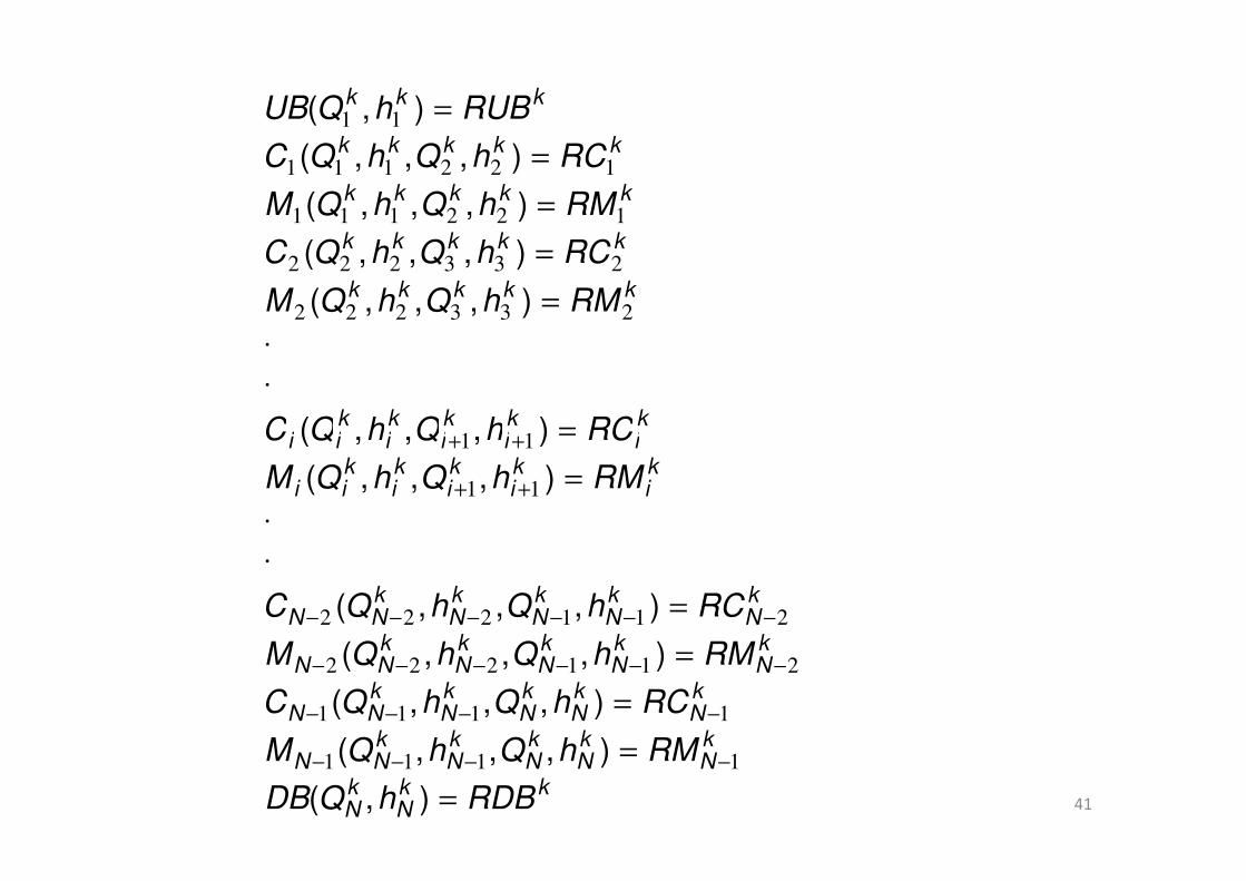
The computational procedure requires a set of trial values to initiate the iterative procedure. These trial values of Q and h can be the initial conditions (if j=1) or the values from the previous time step (if j>1). Solving this set of equations results in 2N residuals. For kth iteration, these residuals can be expressed as
ki
ki
ki
ki
kii
kkkkk
kkkkk
kkkkk
kkkkk
kkk
RChQhQC
RMhQhQM
RChQhQC
RMhQhQM
RChQhQC
RUBhQUB
=
⋅
⋅
=
=
=
=
=
++ ),,,(
),,,(
),,,(
),,,(
),,,(
),(
11
233222
233222
122111
122111
11
41kk
NkN
kN
kN
kN
kN
kNN
kN
kN
kN
kN
kNN
kN
kN
kN
kN
kNN
kN
kN
kN
kN
kNN
ki
ki
ki
ki
kii
iiiiii
RDBhQDB
RMhQhQM
RChQhQC
RMhQhQM
RChQhQC
RMhQhQM
RChQhQC
=
=
=
=
=
⋅
⋅
=
=
−−−−
−−−−
−−−−−−
−−−−−−
++
++
),(
),,,(
),,,(
),,,(
),,,(
),,,(
),,,(
1111
1111
211222
211222
11
11
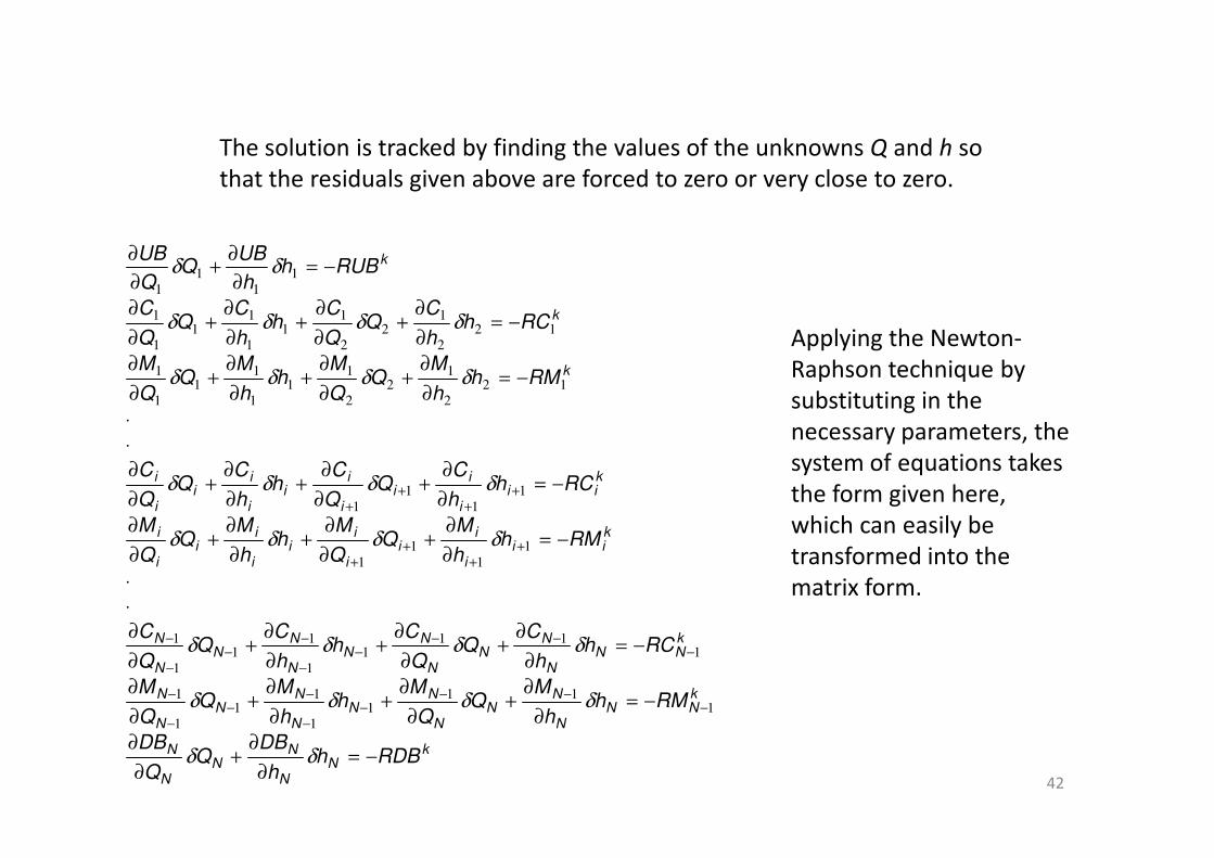
The solution is tracked by finding the values of the unknowns Q and h so that the residuals given above are forced to zero or very close to zero.
k
k
k
RMhh
MQ
Q
Mh
h
MQ
Q
M
RChh
CQ
Q
Ch
h
CQ
Q
C
RUBhh
UBQ
Q
UB
⋅
−=∂
∂+
∂
∂+
∂
∂+
∂
∂
−=∂
∂+
∂
∂+
∂
∂+
∂
∂
−=∂
∂+
∂
∂
δδδδ
δδδδ
δδ
122
12
2
11
1
11
1
1
122
12
2
11
1
11
1
1
11
11
Applying the Newton-Raphson technique by substituting in the necessary parameters, the
42
kN
N
NN
N
N
kNN
N
NN
N
NN
N
NN
N
N
kNN
N
NN
N
NN
N
NN
N
N
kii
i
ii
i
ii
i
ii
i
i
kii
i
ii
i
ii
i
ii
i
i
RDBhh
DBQ
Q
DB
RMhh
MQ
Q
Mh
h
MQ
Q
M
RChh
CQ
Q
Ch
h
CQ
Q
C
RMhh
MQ
Q
Mh
h
MQ
Q
M
RChh
CQ
Q
Ch
h
CQ
Q
C
−=∂
∂+
∂
∂
−=∂
∂+
∂
∂+
∂
∂+
∂
∂
−=∂
∂+
∂
∂+
∂
∂+
∂
∂
⋅
⋅
−=∂
∂+
∂
∂+
∂
∂+
∂
∂
−=∂
∂+
∂
∂+
∂
∂+
∂
∂
⋅
⋅
−−−
−−
−−
−
−
−−−
−−
−−
−
−
++
++
++
++
δδ
δδδδ
δδδδ
δδδδ
δδδδ
111
11
11
1
1
111
11
11
1
1
11
11
11
11
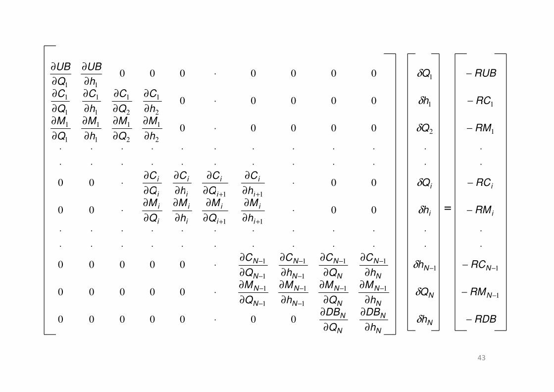
necessary parameters, the system of equations takes the form given here, which can easily be transformed into the matrix form.
RCQh
C
Q
C
h
C
Q
C
RMQh
M
Q
M
h
M
Q
M
RChh
C
Q
C
h
C
Q
C
RUBQh
UB
Q
UB
iii
i
i
i
i
i
i
i
∂∂∂∂
−⋅∂
∂
∂
∂
∂
∂
∂
∂⋅
⋅⋅⋅⋅⋅⋅⋅⋅⋅⋅⋅⋅
⋅⋅⋅⋅⋅⋅⋅⋅⋅⋅⋅⋅
−⋅∂
∂
∂
∂
∂
∂
∂
∂
−⋅∂
∂
∂
∂
∂
∂
∂
∂
−⋅∂
∂
∂
∂
++
δ
δ
δ
δ
0000
00000
00000
0000000
11
122
1
2
1
1
1
1
1
11
2
1
2
1
1
1
1
1
111
43
RDBhh
DB
Q
DB
RMQh
M
Q
M
h
M
Q
M
RChh
C
Q
C
h
C
Q
C
RMhh
M
Q
M
h
M
Q
MhQhQ
NN
N
N
N
NNN
N
N
N
N
N
N
N
NNN
N
N
N
N
N
N
N
iii
i
i
i
i
i
i
i
iiii
−∂
∂
∂
∂⋅
−∂
∂
∂
∂
∂
∂
∂
∂⋅
−∂
∂
∂
∂
∂
∂
∂
∂⋅
⋅⋅⋅⋅⋅⋅⋅⋅⋅⋅⋅⋅
⋅⋅⋅⋅⋅⋅⋅⋅⋅⋅⋅⋅
−⋅∂
∂
∂
∂
∂
∂
∂
∂⋅
∂∂∂∂
−−−
−
−
−
−
−−−−
−
−
−
−
++
++
δ
δ
δ
δ
0000000
00000
00000
0000
111
1
1
1
1
1111
1
1
1
1
11
11
=
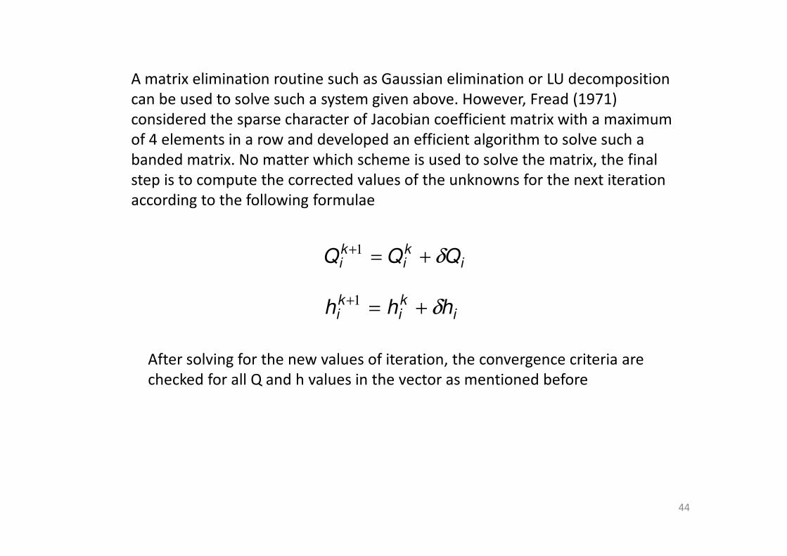
A matrix elimination routine such as Gaussian elimination or LU decomposition can be used to solve such a system given above. However, Fread (1971) considered the sparse character of Jacobian coefficient matrix with a maximum of 4 elements in a row and developed an efficient algorithm to solve such a banded matrix. No matter which scheme is used to solve the matrix, the final step is to compute the corrected values of the unknowns for the next iteration according to the following formulae
iki
ki QQQ δ+=+1
44
iki
ki hhh δ+=+1
After solving for the new values of iteration, the convergence criteria are checked for all Q and h values in the vector as mentioned before
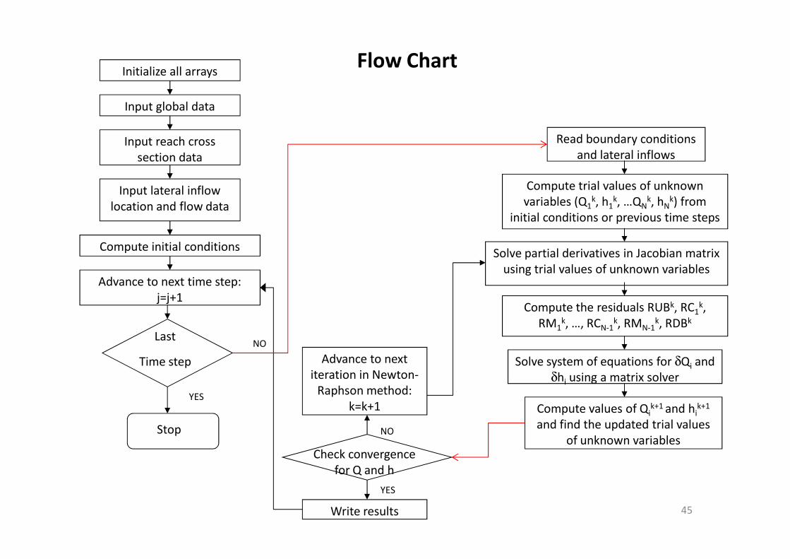
Initialize all arrays
Input global data
Input reach crosssection data
Input lateral inflowlocation and flow data
Compute initial conditions
Advance to next time step:
Read boundary conditionsand lateral inflows
Compute trial values of unknownvariables (Q1
k, h1k, …QN
k, hNk) from
initial conditions or previous time steps
Solve partial derivatives in Jacobian matrixusing trial values of unknown variables
Flow Chart
45
Advance to next time step: j=j+1
Last
Time step
NO
YES
Stop
Advance to nextiteration in Newton-
Raphson method: k=k+1
Check convergencefor Q and h
NO
YES
Write results
Compute the residuals RUBk, RC1k,
RM1k, …, RCN-1
k, RMN-1k, RDBk
Solve system of equations for δQi andδhi using a matrix solver
Compute values of Qik+1 and hi
k+1
and find the updated trial valuesof unknown variables
Reference
Gündüz, O. (2004). Coupled Flow and Contaminant Transport Modeling in
Large Watersheds. Ph.D. Dissertation, School of Civil and Environmental Engineering, Georgia Institute of Technology, Atlanta, GA, USA, 467p
46