NUMERICAL SIMULATION OF VISCOUS FLOW AROUND A TANKER …
17
Brodogradnja/Shipbilding/Open access Volume 68 Number 2, 2017 109 Andrea Farkas Nastia Degiuli Ivana Martić http://dx.doi.org/10.21278/brod68208 ISSN 0007-215X eISSN 1845-5859 NUMERICAL SIMULATION OF VISCOUS FLOW AROUND A TANKER MODEL UDC 629.5.015.2:629.5.018:629.543 Original scientific paper Summary In this paper, numerical simulation of viscous flow around a tanker model was carried out utilizing software package STAR-CCM+. A mathematical model based on Reynolds Averaged Navier-Stokes equations, a k-ε turbulence model and Volume of Fluid method for describing the motion of two-phase media are given. Necessary boundary conditions for the mathematical model and the method of discretization are also described. The effect of grid density on the numerical results for the total resistance of the tanker model was investigated using three different grid densities. Two different types of the k-ε turbulence model were implemented and deviations in the numerical results are highlighted. The results for the total resistance of the tanker model, obtained by numerical simulations, were validated against the experimental results. The experiments were performed in the towing tank of the Brodarski Institute for a wide range of Froude numbers. It was shown that for all three grid densities and for both types of the k-ε turbulence model satisfactory agreement with the experimental results can be achieved for the whole range of Froude numbers. The scale effects were investigated by a Computational Fluid Dynamics study for the same tanker model in three different scales. Numerically calculated scale effects on wave resistance are reviewed. Key words: Computational Fluid Dynamics; Reynolds Averaged Navier-Stokes equations; Volume of Fluid method; k-ε turbulence model; total resistance 1. Introduction To determine the characteristics of water flow around a ship hull, numerical and physical models, i.e. numerical and experimental methods, are most commonly used nowadays. A combination of these methods, together with the results of full-scale trials, is the best way of designing a high-quality ship form and of obtaining a reliable estimation of the hydrodynamic characteristics of a new vessel. Conducting experiments with ship models in towing tanks is very expensive and time consuming. With the application of Computational Fluid Dynamics (CFD), it is possible in the early phase of ship design to gain an insight into the details of the flow around the ship hull and to obtain guidance on how to improve a specific ship form or how to choose the most suitable ship form for model testing. Currently, to simulate free surface flow around a ship hull, potential and viscous flow methods are most commonly used. Viscous flow methods give more accurate results in terms
Transcript of NUMERICAL SIMULATION OF VISCOUS FLOW AROUND A TANKER …
Brodogradnja/Shipbilding/Open access Volume 68 Number 2, 2017
109
Andrea Farkas
Nastia Degiuli
Ivana Martić
http://dx.doi.org/10.21278/brod68208 ISSN 0007-215X
eISSN 1845-5859
NUMERICAL SIMULATION OF VISCOUS FLOW AROUND A
TANKER MODEL
UDC 629.5.015.2:629.5.018:629.543
Original scientific paper
Summary
In this paper, numerical simulation of viscous flow around a tanker model was carried out
utilizing software package STAR-CCM+. A mathematical model based on Reynolds Averaged
Navier-Stokes equations, a k-ε turbulence model and Volume of Fluid method for describing
the motion of two-phase media are given. Necessary boundary conditions for the mathematical
model and the method of discretization are also described. The effect of grid density on the
numerical results for the total resistance of the tanker model was investigated using three
different grid densities. Two different types of the k-ε turbulence model were implemented and
deviations in the numerical results are highlighted. The results for the total resistance of the
tanker model, obtained by numerical simulations, were validated against the experimental
results. The experiments were performed in the towing tank of the Brodarski Institute for a wide
range of Froude numbers. It was shown that for all three grid densities and for both types of the
k-ε turbulence model satisfactory agreement with the experimental results can be achieved for
the whole range of Froude numbers. The scale effects were investigated by a Computational
Fluid Dynamics study for the same tanker model in three different scales. Numerically
calculated scale effects on wave resistance are reviewed.
Key words: Computational Fluid Dynamics; Reynolds Averaged Navier-Stokes
equations; Volume of Fluid method; k-ε turbulence model; total resistance
1. Introduction
To determine the characteristics of water flow around a ship hull, numerical and physical
models, i.e. numerical and experimental methods, are most commonly used nowadays. A
combination of these methods, together with the results of full-scale trials, is the best way of
designing a high-quality ship form and of obtaining a reliable estimation of the hydrodynamic
characteristics of a new vessel. Conducting experiments with ship models in towing tanks is
very expensive and time consuming. With the application of Computational Fluid Dynamics
(CFD), it is possible in the early phase of ship design to gain an insight into the details of the
flow around the ship hull and to obtain guidance on how to improve a specific ship form or how
to choose the most suitable ship form for model testing.
Currently, to simulate free surface flow around a ship hull, potential and viscous flow
methods are most commonly used. Viscous flow methods give more accurate results in terms
Andrea Farkas, Nastia Degiuli, Numerical simulation of viscous flow around a tanker model
Ivana Martić
110
of the ship resistance than potential flow methods [1]. The main problem of viscous flow
methods, beside turbulence modelling, is grid dependence, but this problem is expected to be
solved in the future [2]. Enger et al. [3] performed numerical calculations of resistance, trim
and sinkage based on viscous flow for the KRISO Container Ship (KCS) for different Froude
numbers (Fn) in calm water. They investigated the influence of grid refinement and the choice
of the turbulence model on the numerical results. The authors showed that acceptable accuracy
of the total resistance in comparison with the experimental results can be achieved with a
relatively coarse mesh when the grid is well designed and locally refined in critical zones. Deng
et al. [4] investigated factors affecting the ship resistance calculation utilizing CFD with an
emphasis on mesh generation. They concluded that the grid size on the hull surface is the most
influential parameter in the numerical calculation of ship resistance for a monohull vessel.
Banks et al. [5] predicted the components of total resistance for a KCS utilizing CFD. In their
work, friction and pressure resistance are further divided into aero and hydro components. The
influence of the turbulence model on the numerical results was also investigated. The authors
concluded that the Baseline (BSL) Reynolds stress model provided better results than the Shear
Stress Transport (SST) eddy viscosity model. Guo et al. [6] carried out numerical simulations
of viscous flow around a KRISO Very Large Crude Carrier 2 (KVLCC2) model in order to
estimate the influence of grid density and the turbulence model on the numerical results. The
authors used the SST and Explicit Algebraic Stress k-ω (EAS) turbulence model and concluded
that the anisotropic EAS model provided higher accuracy of results. Pereira et al. [7] performed
an extensive verification and validation procedure for the numerical results of flow around a
KVLCC2 obtained using Reynolds Averaged Navier-Stokes (RANS) equations for a model and
full-scale Reynolds number (Rn). The authors selected a wake-fraction and form factor to
illustrate the scale effects. They concluded that deviations between the flow fields at the
propeller plane, obtained using different turbulence models, decrease with the increase of the
Rn, and that the form factor depends on the Rn. Ozdemir et al. [8] assessed the possibility of
utilizing the software package STAR-CCM+ for the design, analysis and feasibility of computer
simulations for a fast ship, by comparing the results of conducted simulations with the
experimental results. The authors used the Standard k-ε turbulence (SKE) model, and the
obtained results showed satisfactory agreement for Fn values below 0.25. For higher values of
Fn, a low Rn turbulence model is recommended. In the end, they concluded that STAR-CCM+
is a very useful tool to predict the ship resistance curve for Fn below 0.25. Ozdemir et al. [9]
investigated the applicability of a CFD code to predict the total resistance coefficient, wake
distributions and wave profiles in wave cuts. For this purpose, they performed numerical
simulations of viscous flow with a free surface around a KCS model. The authors showed that
nominal wake distribution could be obtained relatively precisely, as could a far field wave
pattern. They obtained satisfactory agreement with the experimental results for the total
resistance coefficient using a fine grid.
While most authors use methods based on RANS for the simulation of flow around a ship
hull, discretization methods for a free surface vary considerably. Although very different, all of
them have been used with success. Wackers et al. [10] described three different methods for the
discretization of a free surface. They concluded that the selection of a particular method
depends on the problem to which the method is applied and the requirements of the applied
method.
Azcueta [2] investigated the impact of a near-wall treatment and concluded that the best
results are obtained if the value of the y+ parameter on the first cell next to the wall is around
50.
One of the disadvantages of viscous flow methods with regard to potential flow methods
is the calculation time. Leroyer et al. [11] represented two numerical procedures which can
reduce the required calculation time for solving the RANS equations with the Volume of Fluid
Numerical simulation of viscous flow around a tanker model Andrea Farkas, Nastia Degiuli,
Ivana Martić
111
(VOF) method. By comparing these procedures with classic procedures, the authors showed
that real problems can be solved up to four times faster.
Nowadays, RANS are used to solve many different types of problem regarding free
surface flows. Atlar et al. [12] used RANS and potential flow methods to develop a hull form
for the Deep-V catamaran. The authors investigated the contribution of novel bow and stern
features on the catamaran performance and found that an anti-slamming bulbous bow and
tunnel stern geometry were optimum. Zaghi et al. [13] investigated the influence of a separation
length on the catamaran interference resistance, both experimentally and numerically. They
used RANS to better understand this phenomenon, because RANS can provide more
information in terms of the wave field, surface pressure and velocity field than an experiment.
Tezdogan et al. [14] performed RANS simulations in order to predict motions and added
resistance for a full-scale KCS at a design and slow steaming speed. The conducted simulations
showed that the application of slow steaming can lead to a decrease of up to 52% in effective
power and CO2 emissions compared with the design speed. Qian et al. [15] performed numerical
and experimental investigations on the hydrodynamic performance of a Small Waterplane Area
Twin Hull (SWATH) with inclined struts. The results of numerical computations, performed
using RANS, are validated by comparing the results with the experimental ones. The authors
concluded that inclined struts can reduce the required power for propulsion in the waves by
using wave energy. Bašić et al. [16] used RANS equations and the VOF method in order to
determine the total resistance of an intact and partially flooded tanker due to a large hole in the
bottom of the hull. RANS provided a better understanding of the very complex flow around and
inside the damaged hull. The authors concluded that the proposed CFD model and settings
provided a good prediction of the total resistance of a damaged tanker.
The prediction of full scale resistance is most commonly carried out by one of the
extrapolation methods. Among them, the most commonly used method is the ITTC 1978
performance prediction method. In order to improve this extrapolation method and to better
understand total resistance decomposition, CFD methods can be used. Inviscid CFD methods
require significantly lower computational time than viscous CFD methods, but they usually
overestimate the stern wave field [17]. Grid refinement studies have indicated that wave field
is grid dependent for viscous CFD methods [18]. Viscous effects are more significant for fuller
ships at lower Fn where shorter waves are present. Therefore, denser grids are needed for
resolving the wave pattern than for higher Fn. Consequently, simulation time is even further
increased. Ploeg et al. [19] used two different viscous CFD methods in order to simulate free
surface viscous flow around a container ship at the model scale and at full scale. One method
is based on finite volumes, unstructured grids, and wall functions, and uses free surface
capturing (ISIS CFD), while the other is based on finite differences, structured grids, no wall
functions and uses the free surface fitting method (PARNASSOS). The authors compared the
results obtained when two different methods were used with the experimental results and
showed that both methods give very similar results in the computed wave pattern, wake fields
and total resistance. Raven et al. [17] performed extensive research on the CFD-based
prediction of full-scale resistance and scale effects. The authors investigated the scaling of
viscous and wave resistance with the PARNASSOS code and concluded that viscous effects
reduce the stern wave system more significantly at the model scale than at full scale. Therefore,
the wave resistance coefficient is found to be 20% greater at full scale than at the model scale.
In this paper, viscous flow around the tanker model is numerically simulated utilizing the
STAR-CCM+ software package for CFD. The results of the numerical calculations are
compared with the experimental results obtained in the Brodarski Institute [20]. The following
sections present the mathematical and physical models used in numerical simulations, describe
the boundary conditions and the discretization method, and give the results of the conducted
Andrea Farkas, Nastia Degiuli, Numerical simulation of viscous flow around a tanker model
Ivana Martić
112
numerical simulations. The numerical results obtained with three different grid densities and
two different types of the k-ε turbulence model are validated against the experimental results.
Furthermore, the initial tanker model was scaled and two additional models were created. For
these two models, the total resistance values are numerically calculated. The total resistance
values for the three models, obtained with numerical simulations, were extrapolated according
to the procedure described in [21] in order to obtain the total resistance of a full-scale ship and
to investigate the scale effect.
2. Governing equations
Computer codes based on viscous flow solve the law of conservation of momentum and
mass conservation with an accuracy that depends on the characteristics of the computational
model of ship motion on the free surface and computing resources [22]. In the case of free
surface flows, an additional equation, which resolves the VOF problem, is introduced. The law
of conservation of momentum becomes the Navier-Stokes equations after the introduction of
the constitutive equations which represent the non-linear partial differential equations. These
equations have no analytical solution for turbulent flows that are stochastic in nature. Therefore,
the Navier-Stokes and continuity equations are most commonly averaged and solved
numerically. A detailed description of the mathematical model and numerical methods for
solving are presented in [23].
The averaged continuity equation and RANS equations for incompressible flows in index
notation read:
0
i
i
u
x
(1)
iji
i j i j
j i j
u pu u u u
t x x x
(2)
where is the fluid density, iu is the averaged velocity vector, i ju u is the Reynolds
stress tensor, p is the mean pressure and ij is the mean viscous stress tensor defined as
follows:
jiij
j i
uu
x x
(3)
where is the dynamic viscosity.
The problem of modelling the free surface is solved using the VOF method. This method
can model two or more fluids which are immiscible and solve only one set of equations (1) and
(2) for one fluid, by introducing the new parameter i -fraction of i-fluid in the cell. The volume
fraction of one phase is determined according to the continuity equation, and for incompressible
flow reads:
0l l iut
(4)
where l is the fraction of water in a particular cell.
The physical properties of a particular fluid depend on the presence of that fluid in a
particular cell. In a domain where there are only two fluids, fluid 1 and fluid 2, the density is
calculated according to the equation:
Numerical simulation of viscous flow around a tanker model Andrea Farkas, Nastia Degiuli,
Ivana Martić
113
2 1 1 1(1 ) (5)
where 1 is the density of fluid 1, 2 is the density of fluid 2, and
1 is the volume
fraction of fluid 1.
Other physical properties are calculated analogously according to equation (5).
For the discretization of RANS, the Finite Volume Method (FVM) is used. In this paper,
the k-ε turbulence model is used, together with the wall functions for the description of the
turbulence effect on averaged flow. This model is based on two differential equations: one for
the description of turbulent kinetic energy k and one for the turbulent energy dissipation rate ε.
In order to investigate the influence of different turbulence modelling, two different types of
the k-ε turbulence model are used: the Realizable k-ε Two-Layer (RKE2L) model and the
Standard k-ε (SKE) model. SKE is a type of k-ε turbulence model that was defined by Launder
and Spalding [24]. In this paper, the SKE model is combined with the high wall y+ treatment
(wall function type of mesh). The wall function type of mesh represents a mesh in a boundary
layer which is set in order to obtain the value of the y+ parameter in the first cell above 30. The
first cell height is set according to this condition. RKE2L contains a new transport equation for
ε, and the critical coefficient of the model Cµ is expressed as a function of a mean flow and of
turbulence properties rather than as being assumed constant as in the standard model.
Furthermore, this model works with low-Rn type meshes and with wall function type meshes
[25]. The differences between these two types of meshes are explained in Section 4 of this
paper.
3. Geometry and experimental setup
Total resistance of the Panamax tanker model made of wood was measured in the towing
tank of Brodarski Institute [20]. The dimensions of the towing tank are: length 276.3 m, width
12.5m and depth 6.0 m. Considering the dimensions of the towing tank and the ship model
scale, no blockage effects were taken into account. The body plan of the towed model and the
bow and stern contour are shown in Figure 1. The main particulars of the full scale ship and
ship model are given in Table 1. The hull has a block coefficient 0.8BC and a midship section
area coefficient 0.995MC . A total of 24 experiments for Fn in the range of 0.064 to 0.212 was
conducted in calm water. The tanker model and measurement equipment can be seen in Figure
2.
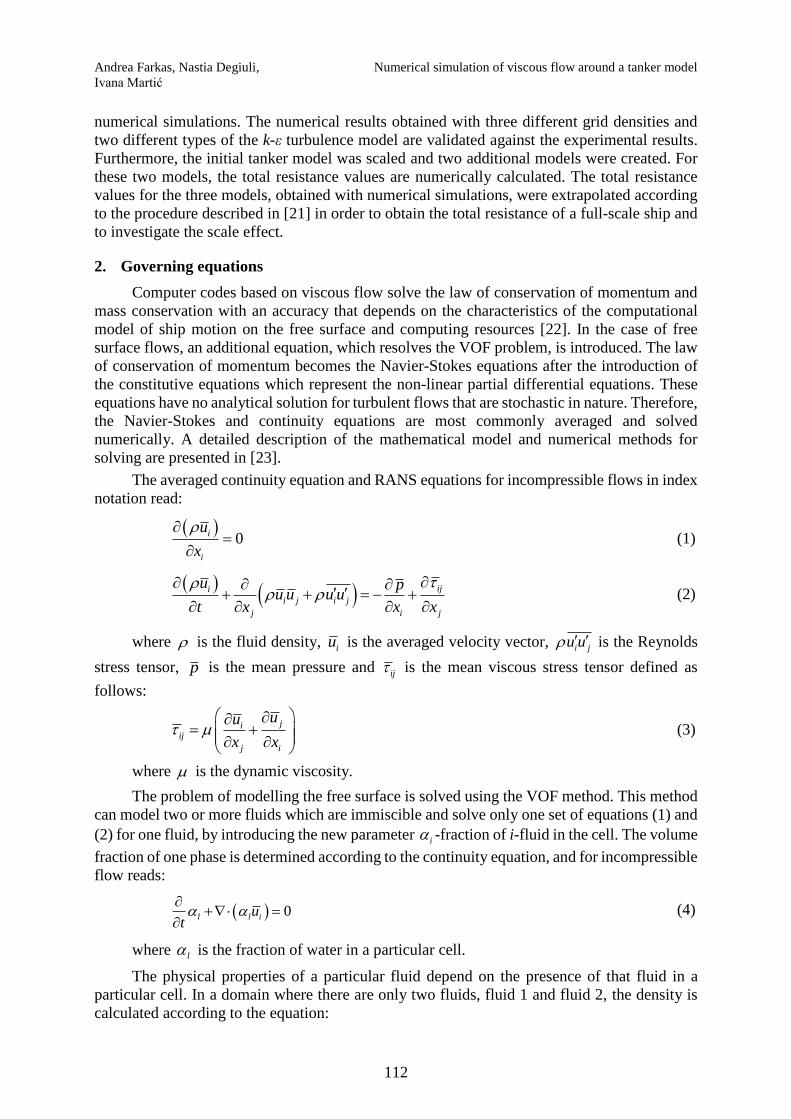
Fig. 1 Body plan, bow and aft contour
Andrea Farkas, Nastia Degiuli, Numerical simulation of viscous flow around a tanker model
Ivana Martić
114
Table 1 Main particulars of the full-scale ship and ship model
Parameter Ship Model
λ (scale) 1 28.814
Lpp 174.8 m 6.0667 m
LWL 178.4 m 6.1917 m
B 32.2 m 1.1176 m
T 12.9 m 0.4477 m
Δ 60829 t 2.4788 t
S (wetted surface) 8749.3 m2 10.5389 m2
xCG (from amidships) 2.54 m 0.0882 m
yCG 0 m 0 m
zCG 6.74 m 0.2341 m
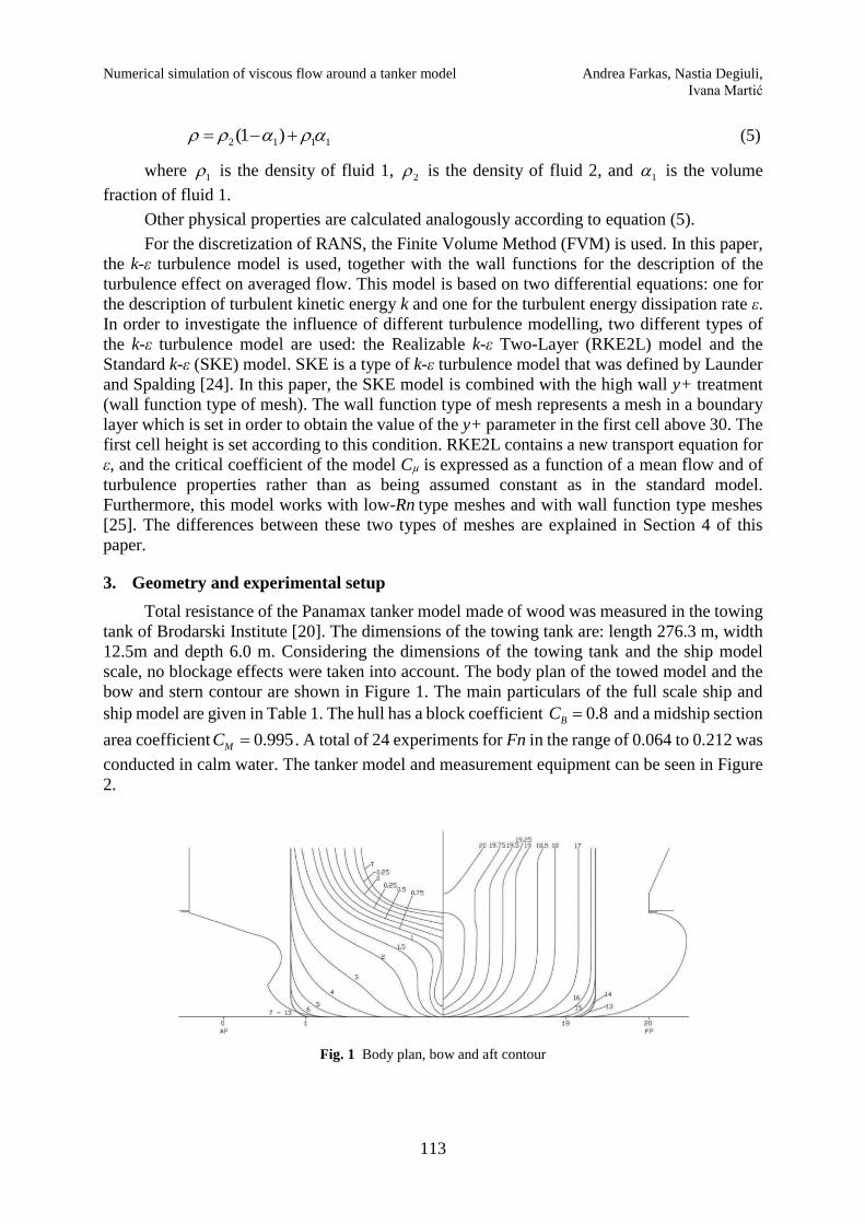
Fig. 2 Towing tank experiment with tanker model [20]
4. Numerical setup
Numerical simulation of viscous flow around the tanker model is carried out utilizing the
software package STAR-CCM+. Creating a computer model begins with the domain creation
around a ship model. The distance of the domain boundaries from the ship model in literature
vary considerably [14]. In this research, the domain boundaries are set to the length Lpp of the
ship model in all directions. Due to the symmetry of the ship model, only half of the
computational domain was modelled. Then a surface mesh was created and remeshed within
the software package STAR-CCM+, using the surface remesher tool. Discretization using FVM
begins with the creation of a surface mesh that consists of faces.
In this paper, the domain is meshed using a surface remesher, trimmer and prism layer
mesher. All mesh parameters are defined as relative values of the cell base size, except in the
case of the prism layer mesher, where the prism layer thickness is set at an absolute value. The
effect of the grid density on the numerical results is investigated using three different grid
densities obtained by changing the cell base size and with the RKE2L turbulence model.
Furthermore, the effect of different types of the k-ε turbulence model on the numerical results
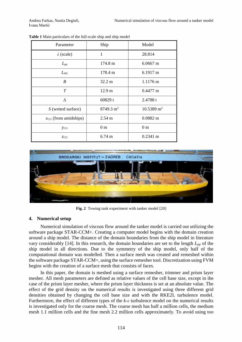
is investigated only for the coarse mesh. The coarse mesh has half a million cells, the medium
mesh 1.1 million cells and the fine mesh 2.2 million cells approximately. To avoid using too
Numerical simulation of viscous flow around a tanker model Andrea Farkas, Nastia Degiuli,
Ivana Martić
115
dense a grid in areas where it is not necessary, additional parts were created with different
conditions of discretization. By applying these refinements, the obtained mesh can capture some
flow characteristics, for example the Kelvin wake or flow separation. In the boundary layer,
where the velocity gradients are high, a prism layer with six cells was created. As mentioned
above, the thickness of this layer is given as an absolute value to achieve a y+ parameter value
around 50 in the first cell next to the wall. The structure of the coarse and fine mesh is shown
in Figure 3.
a) structure of the fine mesh
b) structure of the coarse mesh
c) domain discretization using fine mesh d) domain discretization using coarse mesh
Fig. 3 Discretized computational domain
The mesh is evaluated using two parameters: y+ and the Courant number. The value of
the y+ parameter in the first cell next to the wall should be in the range of 30 to 1000 for the
wall function types of meshes, but since in some cells this cannot be achieved, smaller values
of the y+ parameter are also acceptable. For low-Rn types of meshes, the y+ parameter in the
first cell next to the wall should be around 1 [25]. Wall function types of meshes are chosen for
meshing near the wall, for both types of turbulence models, in order to have a lower total
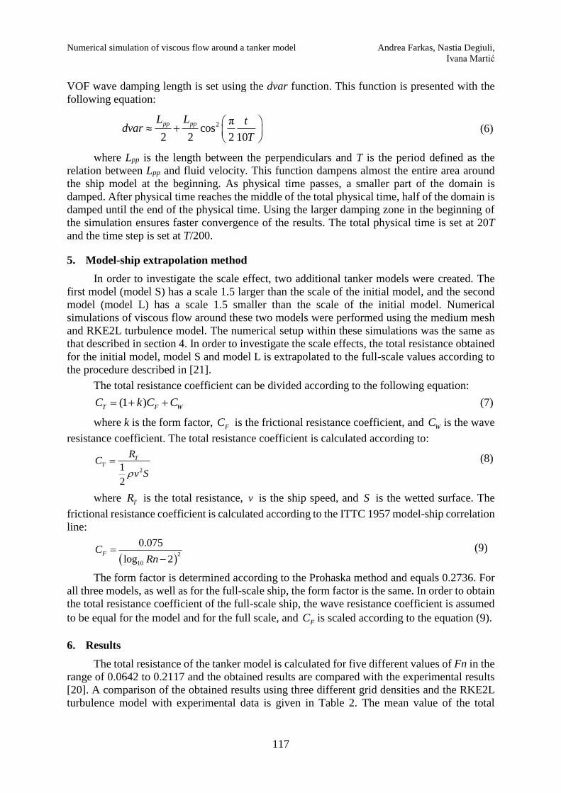
number of cells. The Courant number is defined as a relation of the time step and the time
required for fluid to pass a certain cell with its local speed. Its value should be less than 1 to
have a simulation which requires less calculation time and has higher stability [8]. Coupling the
pressure and velocity field was done with an implicit unsteady solver. It is important to mention
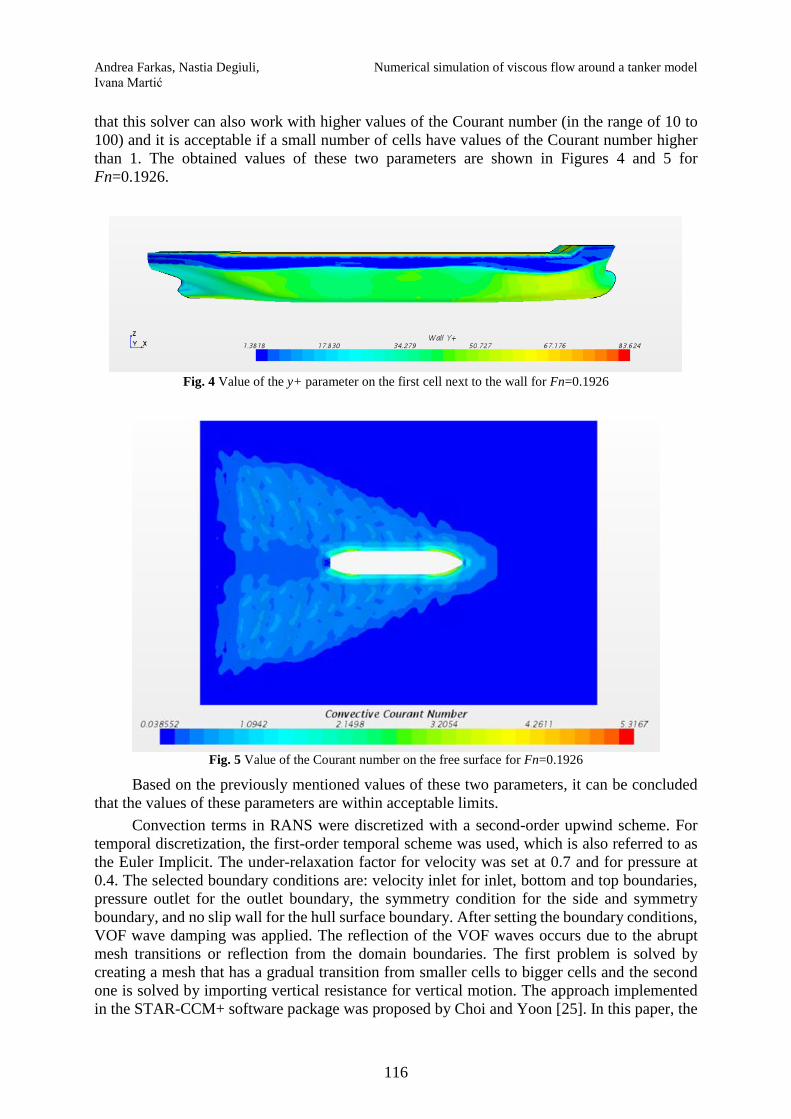
Andrea Farkas, Nastia Degiuli, Numerical simulation of viscous flow around a tanker model
Ivana Martić
116
that this solver can also work with higher values of the Courant number (in the range of 10 to
100) and it is acceptable if a small number of cells have values of the Courant number higher
than 1. The obtained values of these two parameters are shown in Figures 4 and 5 for
Fn=0.1926.
Fig. 4 Value of the y+ parameter on the first cell next to the wall for Fn=0.1926
Fig. 5 Value of the Courant number on the free surface for Fn=0.1926
Based on the previously mentioned values of these two parameters, it can be concluded
that the values of these parameters are within acceptable limits.
Convection terms in RANS were discretized with a second-order upwind scheme. For
temporal discretization, the first-order temporal scheme was used, which is also referred to as
the Euler Implicit. The under-relaxation factor for velocity was set at 0.7 and for pressure at
0.4. The selected boundary conditions are: velocity inlet for inlet, bottom and top boundaries,
pressure outlet for the outlet boundary, the symmetry condition for the side and symmetry
boundary, and no slip wall for the hull surface boundary. After setting the boundary conditions,
VOF wave damping was applied. The reflection of the VOF waves occurs due to the abrupt
mesh transitions or reflection from the domain boundaries. The first problem is solved by
creating a mesh that has a gradual transition from smaller cells to bigger cells and the second
one is solved by importing vertical resistance for vertical motion. The approach implemented
in the STAR-CCM+ software package was proposed by Choi and Yoon [25]. In this paper, the
Numerical simulation of viscous flow around a tanker model Andrea Farkas, Nastia Degiuli,
Ivana Martić
117
VOF wave damping length is set using the dvar function. This function is presented with the
following equation:
2 πcos
2 2 2 10
pp ppL L tdvar
T
(6)
where Lpp is the length between the perpendiculars and T is the period defined as the
relation between Lpp and fluid velocity. This function dampens almost the entire area around
the ship model at the beginning. As physical time passes, a smaller part of the domain is
damped. After physical time reaches the middle of the total physical time, half of the domain is
damped until the end of the physical time. Using the larger damping zone in the beginning of
the simulation ensures faster convergence of the results. The total physical time is set at 20T
and the time step is set at T/200.
5. Model-ship extrapolation method
In order to investigate the scale effect, two additional tanker models were created. The
first model (model S) has a scale 1.5 larger than the scale of the initial model, and the second
model (model L) has a scale 1.5 smaller than the scale of the initial model. Numerical
simulations of viscous flow around these two models were performed using the medium mesh
and RKE2L turbulence model. The numerical setup within these simulations was the same as
that described in section 4. In order to investigate the scale effects, the total resistance obtained
for the initial model, model S and model L is extrapolated to the full-scale values according to
the procedure described in [21].
The total resistance coefficient can be divided according to the following equation:
(1 )T F WC k C C (7)
where k is the form factor, FC is the frictional resistance coefficient, and WC is the wave
resistance coefficient. The total resistance coefficient is calculated according to:
21
2
TT
RC
v S
(8)
where TR is the total resistance, v is the ship speed, and S is the wetted surface. The
frictional resistance coefficient is calculated according to the ITTC 1957 model-ship correlation
line:
2
10
0.075
log 2FC
Rn
(9)
The form factor is determined according to the Prohaska method and equals 0.2736. For
all three models, as well as for the full-scale ship, the form factor is the same. In order to obtain
the total resistance coefficient of the full-scale ship, the wave resistance coefficient is assumed
to be equal for the model and for the full scale, and FC is scaled according to the equation (9).
6. Results
The total resistance of the tanker model is calculated for five different values of Fn in the
range of 0.0642 to 0.2117 and the obtained results are compared with the experimental results
[20]. A comparison of the obtained results using three different grid densities and the RKE2L
turbulence model with experimental data is given in Table 2. The mean value of the total
Andrea Farkas, Nastia Degiuli, Numerical simulation of viscous flow around a tanker model
Ivana Martić
118
resistance force is calculated, but taking into account only the values of the last 20% of physical
time. Relative deviations are calculated according to the following equation:
CFD EXP
EXP% 100T T
T
R RRD
R
(10)
where CFD
TR is the total resistance obtained numerically and EXP
TR is the total resistance
obtained experimentally.
If the relative deviation is positive, the result obtained with numerical simulation
overestimates the measured value, and if it is negative, the result obtained with numerical
simulation underestimates the measured value. The results obtained with numerical simulations
show satisfactory agreement with the experimental results. The greatest relative deviation for
fine mesh is 1.35%, for medium mesh 1.90%, and for coarse mesh 2.55%, except for the
smallest value of Fn. These deviations for the smallest values of Fn are larger, i.e., 8.14% for
coarse mesh, 5.42% for medium mesh, and 4.23% for fine mesh. It is important to remark that
for the smallest value of Fn, a physical wave pattern was not obtained. Fine mesh with 2.2
million cells was not sufficient to capture the wave pattern for such a small value of Fn, because
the obtained wave elevations were around 2 mm. It is necessary to use mesh with a larger
number of cells to capture waves. The obtained relative deviations would have been smaller if
mesh with a larger number of cells was used, but this would significantly increase the
calculation time. Frictional resistance decreased for this value of Fn when mesh with a larger
number of cells was used. For the smallest value of Fn, frictional resistance has a significantly
higher proportion in the total resistance than the pressure resistance (numerically obtained
frictional resistance is 80% of the total resistance). Since the value of the frictional resistance
obtained with numerical simulations using a larger number of cells decreases, the value of the
total resistance also decreases and thus converges to the total resistance value obtained with
measurements [26]. In addition, for small values of Fn it is possible to ignore the wave
resistance and to carry out simulation for a deeply immersed body according to ITTC
recommendations [27].
The total resistance coefficient CT curve as a function of Fn obtained by numerical
simulations and experimentally is shown in Figure 6.
Table 2 Comparison between experimentally and numerically obtained total resistance values
Fn v, m/s
RT EXP, N
RT CFD, N,
(Relative deviation, %)
Experiment Coarse mesh Medium mesh Fine mesh
0.0642 0.5001 6.093 6.589
(+8.137)
6.423
(+5.422)
6.351
(+4.227)
0.1283 0.9999 22.937 23.121
(+0.804)
23.010
(+0.320)
22.879
(-0.251)
0.1669 1.3002 38.147 38.028
(-0.311)
37.912
(-0.615)
37.934
(-0.558)
0.1926 1.5008 53.461 52.435
(-1.920)
52.448
(-1.895)
52.741
(-1.346)
0.2117 1.6499 67.639 65.909
(-2.558)
67.036
(-0.891)
68.041
(+0.594)
Numerical simulation of viscous flow around a tanker model Andrea Farkas, Nastia Degiuli,
Ivana Martić
119
Fig. 6 Curve of the total resistance coefficient as a function of Fn
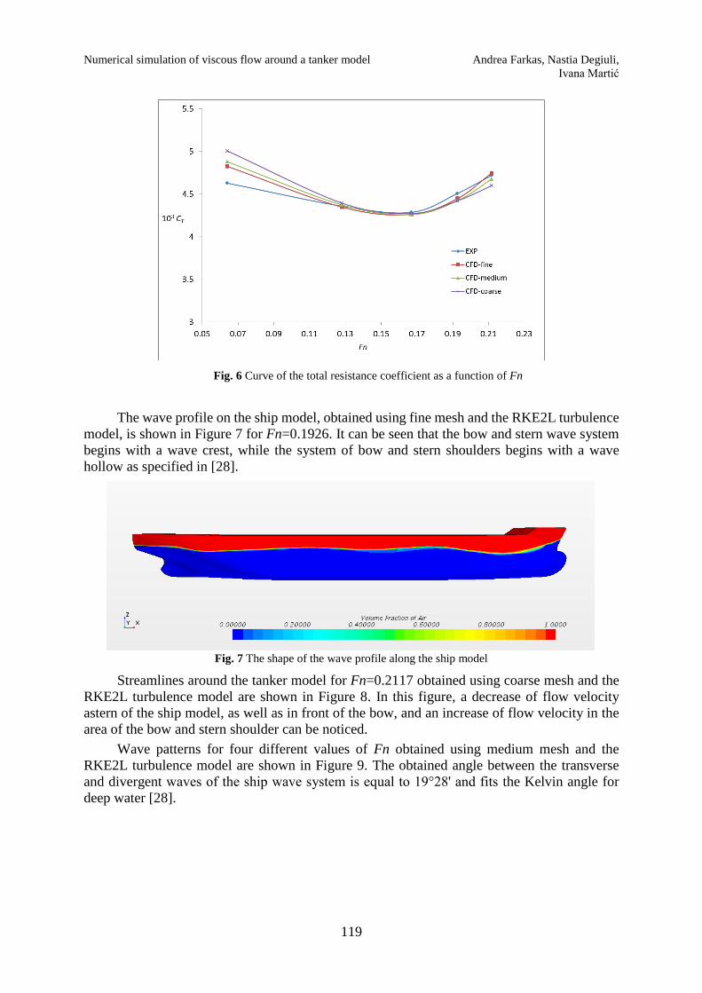
The wave profile on the ship model, obtained using fine mesh and the RKE2L turbulence
model, is shown in Figure 7 for Fn=0.1926. It can be seen that the bow and stern wave system
begins with a wave crest, while the system of bow and stern shoulders begins with a wave
hollow as specified in [28].
Fig. 7 The shape of the wave profile along the ship model
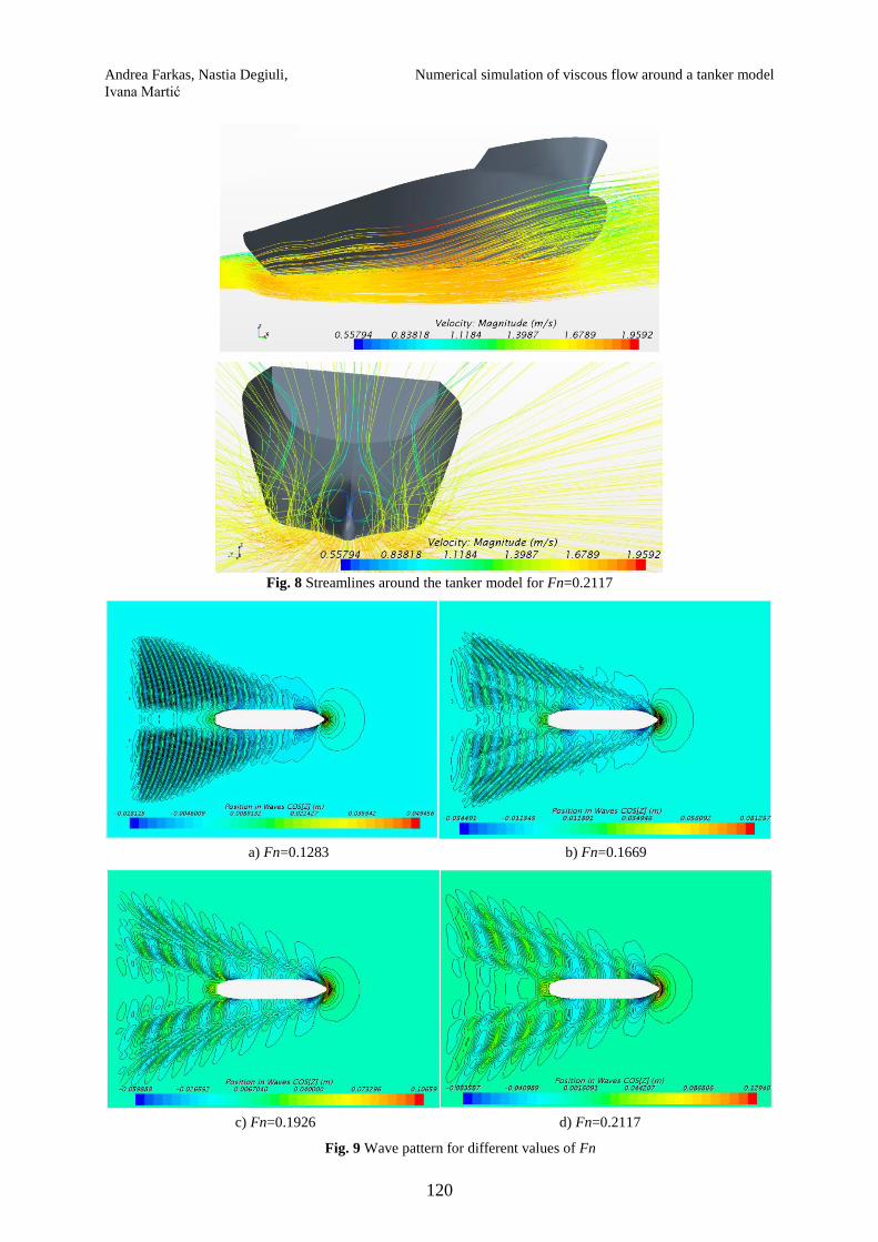
Streamlines around the tanker model for Fn=0.2117 obtained using coarse mesh and the
RKE2L turbulence model are shown in Figure 8. In this figure, a decrease of flow velocity
astern of the ship model, as well as in front of the bow, and an increase of flow velocity in the
area of the bow and stern shoulder can be noticed.
Wave patterns for four different values of Fn obtained using medium mesh and the
RKE2L turbulence model are shown in Figure 9. The obtained angle between the transverse
and divergent waves of the ship wave system is equal to 19°28' and fits the Kelvin angle for
deep water [28].
Andrea Farkas, Nastia Degiuli, Numerical simulation of viscous flow around a tanker model
Ivana Martić
120
Fig. 8 Streamlines around the tanker model for Fn=0.2117
a) Fn=0.1283 b) Fn=0.1669
c) Fn=0.1926 d) Fn=0.2117
Fig. 9 Wave pattern for different values of Fn
Numerical simulation of viscous flow around a tanker model Andrea Farkas, Nastia Degiuli,
Ivana Martić
121
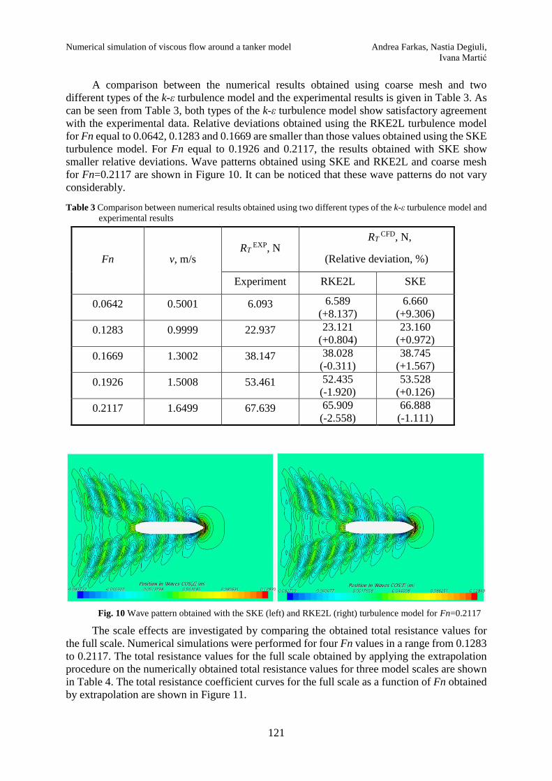
A comparison between the numerical results obtained using coarse mesh and two
different types of the k-ε turbulence model and the experimental results is given in Table 3. As
can be seen from Table 3, both types of the k-ε turbulence model show satisfactory agreement
with the experimental data. Relative deviations obtained using the RKE2L turbulence model
for Fn equal to 0.0642, 0.1283 and 0.1669 are smaller than those values obtained using the SKE
turbulence model. For Fn equal to 0.1926 and 0.2117, the results obtained with SKE show
smaller relative deviations. Wave patterns obtained using SKE and RKE2L and coarse mesh
for Fn=0.2117 are shown in Figure 10. It can be noticed that these wave patterns do not vary
considerably.
Table 3 Comparison between numerical results obtained using two different types of the k-ε turbulence model and
experimental results
Fn v, m/s RT
EXP, N RT
CFD, N,
(Relative deviation, %)
Experiment RKE2L SKE
0.0642 0.5001 6.093 6.589
(+8.137)
6.660
(+9.306)
0.1283 0.9999 22.937 23.121
(+0.804)
23.160
(+0.972)
0.1669 1.3002 38.147 38.028
(-0.311)
38.745
(+1.567)
0.1926 1.5008 53.461 52.435
(-1.920)
53.528
(+0.126)
0.2117 1.6499 67.639 65.909
(-2.558)
66.888
(-1.111)
Fig. 10 Wave pattern obtained with the SKE (left) and RKE2L (right) turbulence model for Fn=0.2117
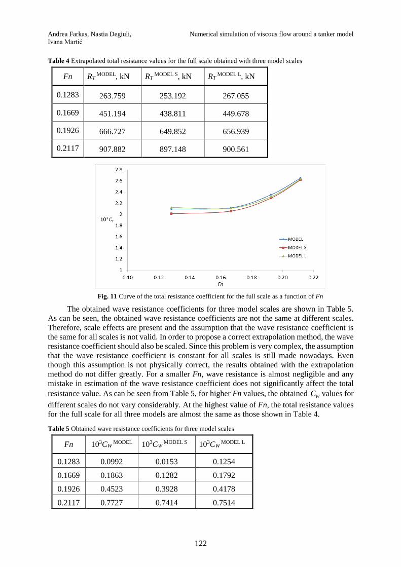
The scale effects are investigated by comparing the obtained total resistance values for
the full scale. Numerical simulations were performed for four Fn values in a range from 0.1283
to 0.2117. The total resistance values for the full scale obtained by applying the extrapolation
procedure on the numerically obtained total resistance values for three model scales are shown
in Table 4. The total resistance coefficient curves for the full scale as a function of Fn obtained
by extrapolation are shown in Figure 11.
Andrea Farkas, Nastia Degiuli, Numerical simulation of viscous flow around a tanker model
Ivana Martić
122
Table 4 Extrapolated total resistance values for the full scale obtained with three model scales
Fn RT MODEL, kN RT
MODEL S, kN RT MODEL L, kN
0.1283 263.759 253.192 267.055
0.1669 451.194 438.811 449.678
0.1926 666.727 649.852 656.939
0.2117 907.882 897.148 900.561
Fig. 11 Curve of the total resistance coefficient for the full scale as a function of Fn
The obtained wave resistance coefficients for three model scales are shown in Table 5.
As can be seen, the obtained wave resistance coefficients are not the same at different scales.
Therefore, scale effects are present and the assumption that the wave resistance coefficient is
the same for all scales is not valid. In order to propose a correct extrapolation method, the wave
resistance coefficient should also be scaled. Since this problem is very complex, the assumption
that the wave resistance coefficient is constant for all scales is still made nowadays. Even
though this assumption is not physically correct, the results obtained with the extrapolation
method do not differ greatly. For a smaller Fn, wave resistance is almost negligible and any
mistake in estimation of the wave resistance coefficient does not significantly affect the total
resistance value. As can be seen from Table 5, for higher Fn values, the obtained WC values for
different scales do not vary considerably. At the highest value of Fn, the total resistance values
for the full scale for all three models are almost the same as those shown in Table 4.
Table 5 Obtained wave resistance coefficients for three model scales
Fn 103CW MODEL 103CW
MODEL S 103CW
MODEL L
0.1283 0.0992 0.0153 0.1254
0.1669 0.1863 0.1282 0.1792
0.1926 0.4523 0.3928 0.4178
0.2117 0.7727 0.7414 0.7514
Numerical simulation of viscous flow around a tanker model Andrea Farkas, Nastia Degiuli,
Ivana Martić
123
7. Conclusion
In this paper, numerical simulations of viscous flow around a tanker model were
performed. The k-ε turbulence model with wall functions was used. Cells near the wall were
adjusted in order to achieve y+ parameter values around 50. The effect of the grid density on
the numerical results was investigated using three different grid densities. The obtained results
of the conducted numerical simulations show that it is possible to achieve satisfactory
agreement with the experimental results even though a lower number of cells is used, greatly
reducing the calculation time as a result. For example, calculation using fine mesh lasts about
five times longer than calculation using coarse mesh. The greatest relative deviation for fine
mesh is 1.35%, for medium mesh 1.90% and for coarse mesh 2.55%, except for the smallest
value of Fn. These deviations for the smallest values of Fn are larger, i.e., 8.14% for coarse
mesh, 5.42% for medium mesh and 4.23% for fine mesh. By using a grid with a larger number
of cells, smaller relative deviation would be obtained, but the calculation time would increase
considerably. The effect of two different types of the k-ε turbulence model on the numerical
results was investigated using the SKE and RKE2L turbulence model. This investigation was
performed for the coarse mesh and the obtained results showed satisfactory agreement for both
types of the k-ε turbulence model. In this paper, the scale effects were investigated by
comparing the total resistance values for the full scale obtained by extrapolating the results of
numerical simulations for three different model scales. Since the obtained wave resistance
coefficients for different scales were not the same, the scaling of the wave resistance coefficient
should also be implemented in the extrapolation method in the future. Bearing in mind that
scaling of the wave resistance coefficient is a very complex problem, the wave resistance
coefficient is assumed to be constant for the model and for the ship. Nevertheless, the total
resistance values for the full scale do not differ considerably. CFD studies could provide better
insight into the scaling of wave resistance. This will form part of future work, as will an
investigation of the effect of the turbulence model on the scale effect.
Acknowledgement
The authors would like to thank the Faculty of Mechanical Engineering and Naval
Architecture, University of Zagreb, for funding the licence of the software package STAR-
CCM+ and for co-financing the experiment. The authors are also grateful to Professor Milovan
Perić for useful advice and continuous support, and to the Croatian Science Foundation under
project 8658.
REFERENCES
[1] Ahmed, Y., Soares, C.G.: Simulation of free surface flow around a VLCC hull using viscous and potential
flow methods, Ocean engineering, Vol. 36, No. 9, 2009, pp. 691-696.
https://doi.org/10.1016/j.oceaneng.2009.03.010.
[2] Azcueta Repetto, R.: Computation of Turbulent Free-Surface Flows Around Ships and Floating Bodies,
Doctoral thesis, Technischen Universitat Hamburg, Hamburg, 2001.
[3] Enger, S., Perić, M., Perić, R.: Simulation of flow around KCS-hull, Proceedings from Gothenburg 2010-
A Workshop on Numerical Ship Hydrodynamics, Gothenburg, 2010.
[4] Deng, R., Huang, D.B., Zhou, G.L., Sun, H.W.: Investigating on Some Factors Effecting Ship Resistance
Calculation with CFD Code FLUENT [J], Journal of Ship Mechanics, Vol. 17, No. 6, 2013, pp.616-624.
[5] Banks, J., Phillips, A.B., Turnock, S.: Free surface CFD prediction of components of ship resistance for
KCS, Proceedings of the 13th Numerical Towing Tank Symposium, Duisburg, 2010.
[6] Guo B.J., Deng G.B., Steen S.: Verification and validation of numerical calculation of ship resistance and
flow field of a large tanker, Ships and Offshore Structures, Vol. 8, No. 1, 2013, pp. 3-14.
https://doi.org/10.1080/17445302.2012.669263.
Andrea Farkas, Nastia Degiuli, Numerical simulation of viscous flow around a tanker model
Ivana Martić
124
[7] Pereira, F.S., Eca, L., Vaz, G.: Verification and Validation exercises for the flow around the KVLCC2
tanker at model and full-scale Reynolds numbers, Ocean Engineering, Vol. 129, 2017, pp. 133-148.
https://doi.org/10.1016/j.oceaneng.2016.11.005.
[8] Ozdemir, H.Y., Barlas, B., Yilmaz, T., Bayraktar, S.: Numerical and experimental study of turbulent free
surface flow for a fast ship model, Brodogradnja, Vol. 65, No. 1, 2014, pp.39-54.
[9] Ozdemir, H.Y., Cosgun, T., Dogrul, A., Barlas, B.: A numerical application to predict the resistance and
wave pattern of Kriso Container Ship, Brodogradnja, Vol. 67, No. 2, 2016, pp.47-65.
https://doi.org/10.21278/brod67204.
[10] Wackers, J., Koren, B., Raven, H.C., van der Ploeg, A., Starke, A.R., Deng, G.B., Queutey, P., Visonneau,
M., Hino, T., Ohashi, K.: Free-Surface Viscous Flow Solution Methods for Ship Hydrodynamics, Archives
of Computational Methods in Engineering, Vol. 18, No. 1, 2011, pp.1-41. https://doi.org/10.1007/s11831-
011-9059-4.
[11] Leroyer, A., Wackers, J., Queutey, P., Guilmineau, E.: Numerical strategies to speed up CFD computations
with free surface-Application to the dynamic equilibrium of hulls, Ocean engineering, Vol. 38, No. 17,
2011, pp.2070-2076. https://doi.org/10.1016/j.oceaneng.2011.09.006.
[12] Atlar M., Kwangcheol S., Roderick S., Danisman D.B.: Anti-slamming bulbous bow and tunnel stern
applications on a novel Deep-V catamaran for improved performance, International Journal of Naval
Architecture and Ocean Engineering, Vol. 5, 2013, pp. 302-312. https://doi.org/10.2478/IJNAOE-2013-
0134.
[13] Zaghi, S., Broglia, R., Di Mascio, A.: Analysis of the interference effects for high-speed catamarans by
model tests and numerical simulations, Ocean Engineering, Vol. 38, No. 17, 2011, pp. 2110-2122.
https://doi.org/10.1016/j.oceaneng.2011.09.037.
[14] Tezdogan T., Demirel Y.K., Kellett P., Khorasanchi M., Incecik A. and Turan O.: Full-scale unsteady
RANS CFD simulations of ship behavior and performance in head seas due to slow steaming, Ocean
Engineering, Vol. 97, 2015, pp. 186–206. https://doi.org/10.1016/j.oceaneng.2015.01.011.
[15] Qian, P., Yi, H., Li, Y.: Numerical and experimental studies on hydrodynamic performance of a small-
waterplane-area-twin-hull (SWATH) vehicle with inclined struts, Ocean Engineering, Vol. 96, 2015, pp.
181-191. https://doi.org/10.1016/j.oceaneng.2014.12.039.
[16] Bašić, J., Degiuli, N., Dejhalla, R.: Total resistance prediction of an intact and damaged tanker with flooded
tanks in calm water, Ocean Engineering, Vol. 130, 2017, pp. 83-91.
https://doi.org/10.1016/j.oceaneng.2016.11.034.
[17] Raven, H.C., van der Ploeg, A., Starke, A.R., Eca, L.: Towards a CFD-based prediction of ship performance
--- progress in predicting full-scale resistance and scale effects, Proceedings of RINA-CFD-2008, RINA
MARINE CFD conference, London, 2008.
[18] Raven, H.C., van der Ploeg, A., Starke, B.: Computation of free-surface viscous flows at model and full
scale by a steady iterative approach, 25th Symp. Naval Hydrodynamics, St. John’s, Canada, 2004.
[19] van der Ploeg, A., Raven, H.C., Windt, J., Leroyer, A., Queutey, P., Deng, G., Visonneau, M.: Computation
of free-surface viscous flows at model and full scale – a comparison of two different approaches, Proc. 27th
Symposium on Naval Hydrodynamics, Seoul, Korea, 2008.
[20] Brodarski Institute, Report 6454-M. Tech. rep., Brodarski Institute, 2015, Zagreb.
[21] Molland, A.F., Turnock, S.R., Hudson, D.A.: Ship Resistance and Propulsion: Practical Estimation of Ship
Propulsive Power, Cambridge University Press, Cambridge, 2011.
https://doi.org/10.1017/CBO9780511974113
[22] Agrusta, A., Bruzzone, D., Esposito, C, Zotti, I.: CFD simulations to evaluate the ships resistance:
development of a systematic method with use of low number of cells, Proceedings of 21th Symposium on
the Theory and Practice of Shipbuilding, SORTA 2014, Faculty of engineering, Rijeka, 2014, pp. 277-290..
[23] Ferziger, J.H., Perić, M.: Computational Methods for Fluid Dynamics, Springer Science & Business Media,
Berlin, 2012.
[24] Launder, B.E., Spalding, D.B.: The numerical computation of turbulent flows, Computer methods in
applied mechanics and engineering, Vol. 3, No. 2, 1974, pp. 269-289. https://doi.org/10.1016/0045-
7825(74)90029-2.
[25] STAR-CCM+, User Guide, CD-adapco, 2016.
[26] Farkas, A.: Numerička simulacija viskoznog strujanja oko trupa broda, Master thesis, Faculty of
Mechanical Engineering and Naval Architecture, University of Zagreb, Zagreb, 2016.

Numerical simulation of viscous flow around a tanker model Andrea Farkas, Nastia Degiuli,
Ivana Martić
125
[27] International Towing Tank Conference (ITTC): Practical guidelines for ship CFD applications. Proceedings
of the 26th International Towing Tank Conference, Brazil, 2011.
[28] Larsson, L., Raven, H.C.: Ship Resistance and Flow, The Society of Naval Architects and Marine
Engineers, New Jersey, 2010.125
Submitted: 07.02.2017.
Accepted: 29.03.2017.
Andrea Farkas
Nastia Degiuli, [email protected]
Ivana Martić
University of Zagreb,
Faculty of Mechanical Engineering and Naval Architecture,
Ivana Lučića 5, 10000 Zagreb, Croatia