1/44

JJIIJI

Back

Close

Nonlinear Fiber Optics and itsApplications in Optical Signal Processing

Govind P. AgrawalInstitute of OpticsUniversity of RochesterRochester, NY 14627

c©2007 G. P. Agrawal

2/44

JJIIJI

Back

Close

Outline

• Introduction

• Self-Phase Modulation

• Cross-Phase Modulation

• Four-Wave Mixing

• Stimulated Raman Scattering

• Stimulated Brillouin Scattering

• Concluding Remarks

3/44

JJIIJI

Back

Close

Introduction

Fiber nonlinearities

• Studied during the 1970s.

• Ignored during the 1980s.

• Feared during the 1990s.

• Are being used in this decade.

Objective:

• Review of Nonlinear Effects in Optical Fibers.

4/44

JJIIJI

Back

Close

Major Nonlinear Effects

• Self-Phase Modulation (SPM)

• Cross-Phase Modulation (XPM)

• Four-Wave Mixing (FWM)

• Stimulated Raman Scattering (SRS)

• Stimulated Brillouin Scattering (SBS)

Origin of Nonlinear Effects in Optical Fibers

• Ultrafast third-order susceptibility χ (3).

• Real part leads to SPM, XPM, and FWM.

• Imaginary part leads to SBS and SRS.

5/44

JJIIJI

Back

Close

Self-Phase Modulation

• Refractive index depends on optical intensity as (Kerr effect)

n(ω, I) = n0(ω)+n2I(t).

• Frequency dependence leads to dispersion and pulse broadening.

• Intensity dependence leads to nonlinear phase shift

φNL(t) = (2π/λ )n2I(t)L.

• An optical field modifies its own phase (thus, SPM).

• Phase shift varies with time for pulses (chirping).

• As a pulse propagates along the fiber, its spectrum changes

because of SPM.

6/44

JJIIJI

Back

Close

Nonlinear Phase Shift• Pulse propagation governed by Nonlinear Schrodinger Equation

i∂A∂ z− β2

2∂ 2A∂ t2 + γ|A|2A = 0.

• Dispersive effects within the fiber included through β2.

• Nonlinear effects included through γ = 2πn2/(λAeff).

• If we ignore dispersive effects, solution can be written as

A(L, t) = A(0, t)exp(iφNL), where φNL(t) = γL|A(0, t)|2.

• Nonlinear phase shift depends on input pulse shape.

• Maximum Phase shift: φmax = γP0L = L/LNL.

• Nonlinear length: LNL = (γP0)−1 ∼ 1 km for P0 ∼ 1 W.

7/44

JJIIJI

Back

Close

SPM-Induced Chirp

−2 −1 0 1 20

0.2

0.4

0.6

0.8

1

Time, T/T0

Pha

se, φ

NL

−2 −1 0 1 2

−2

−1

0

1

2

Time, T/T0

Chi

rp, δ

ωT

0

(a) (b)

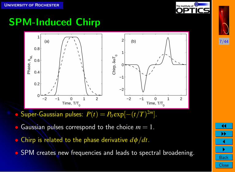
• Super-Gaussian pulses: P(t) = P0 exp[−(t/T )2m].

• Gaussian pulses correspond to the choice m = 1.

• Chirp is related to the phase derivative dφ/dt.

• SPM creates new frequencies and leads to spectral broadening.

8/44

JJIIJI

Back

Close

SPM-Induced Spectral Broadening

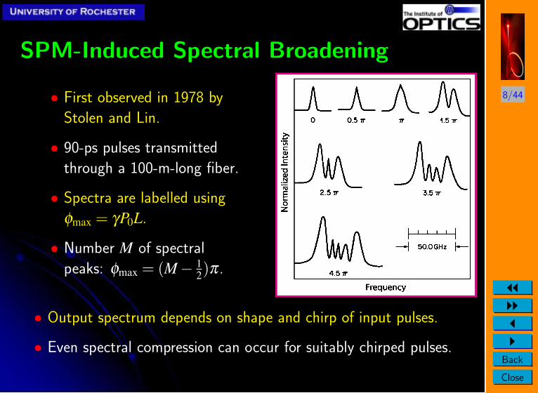
• First observed in 1978 by

Stolen and Lin.

• 90-ps pulses transmitted

through a 100-m-long fiber.

• Spectra are labelled using

φmax = γP0L.

• Number M of spectral

peaks: φmax = (M− 12)π .

• Output spectrum depends on shape and chirp of input pulses.

• Even spectral compression can occur for suitably chirped pulses.

9/44

JJIIJI

Back

Close

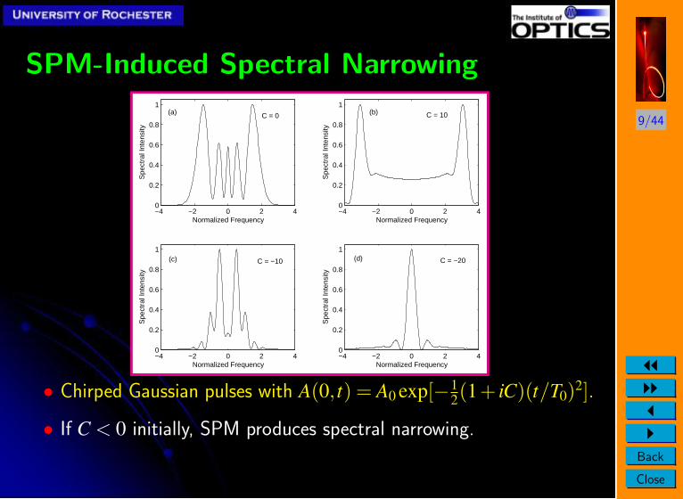
SPM-Induced Spectral Narrowing

−4 −2 0 2 40

0.2

0.4

0.6

0.8

1

Normalized Frequency

Spe

ctra

l Int

ensi

ty

−4 −2 0 2 40

0.2

0.4

0.6

0.8

1

Normalized Frequency

Spe

ctra

l Int

ensi

ty

−4 −2 0 2 40

0.2

0.4

0.6

0.8

1

Normalized Frequency

Spe

ctra

l Int

ensi

ty

−4 −2 0 2 40

0.2

0.4

0.6

0.8

1

Normalized Frequency

Spe

ctra

l Int

ensi

ty

C = 0 C = 10

C = −10 C = −20

(a) (b)

(c) (d)

• Chirped Gaussian pulses with A(0, t) = A0 exp[−12(1+ iC)(t/T0)2].

• If C < 0 initially, SPM produces spectral narrowing.

10/44

JJIIJI

Back

Close

SPM: Good or Bad?• SPM-induced spectral broadening can degrade performance of a

lightwave system.

• Modulation instability often enhances system noise.

On the positive side . . .

• Modulation instability can be used to produce ultrashort pulses at

high repetition rates.

• SPM often used for fast optical switching (NOLM or MZI).

• Formation of standard and dispersion-managed optical solitons.

• Useful for all-optical regeneration of WDM channels.

• Other applications (pulse compression, chirped-pulse amplification,

passive mode-locking, etc.)

11/44

JJIIJI

Back

Close

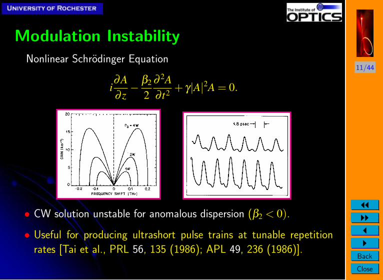
Modulation InstabilityNonlinear Schrodinger Equation

i∂A∂ z− β2

2∂ 2A∂ t2 + γ|A|2A = 0.

• CW solution unstable for anomalous dispersion (β2 < 0).

• Useful for producing ultrashort pulse trains at tunable repetition

rates [Tai et al., PRL 56, 135 (1986); APL 49, 236 (1986)].

12/44

JJIIJI

Back

Close

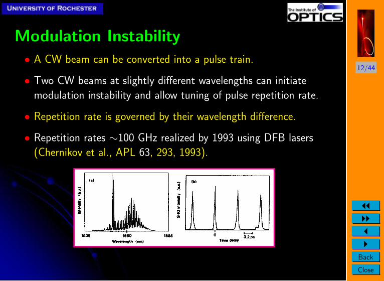
Modulation Instability

• A CW beam can be converted into a pulse train.

• Two CW beams at slightly different wavelengths can initiate

modulation instability and allow tuning of pulse repetition rate.

• Repetition rate is governed by their wavelength difference.

• Repetition rates ∼100 GHz realized by 1993 using DFB lasers

(Chernikov et al., APL 63, 293, 1993).

13/44

JJIIJI

Back

Close

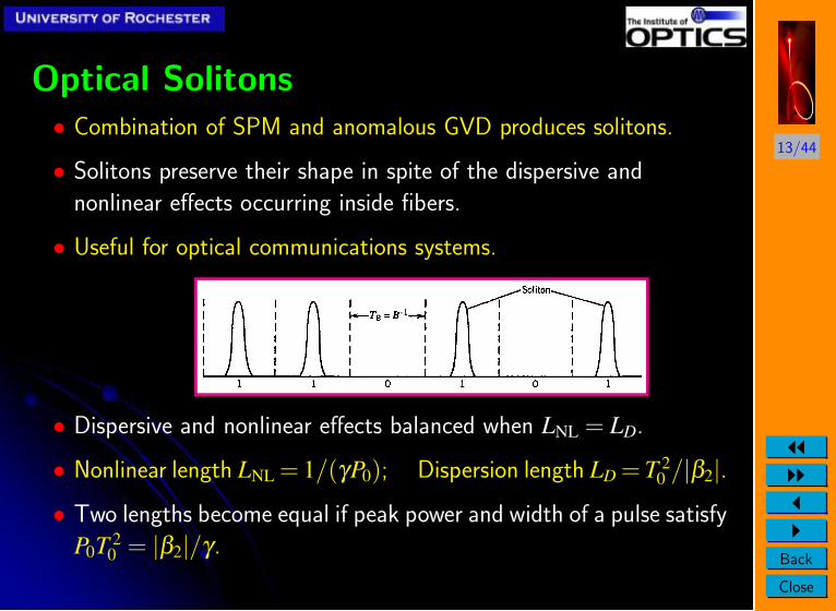
Optical Solitons• Combination of SPM and anomalous GVD produces solitons.

• Solitons preserve their shape in spite of the dispersive and

nonlinear effects occurring inside fibers.

• Useful for optical communications systems.

• Dispersive and nonlinear effects balanced when LNL = LD.

• Nonlinear length LNL = 1/(γP0); Dispersion length LD = T 20 /|β2|.

• Two lengths become equal if peak power and width of a pulse satisfy

P0T 20 = |β2|/γ .

14/44

JJIIJI

Back

Close

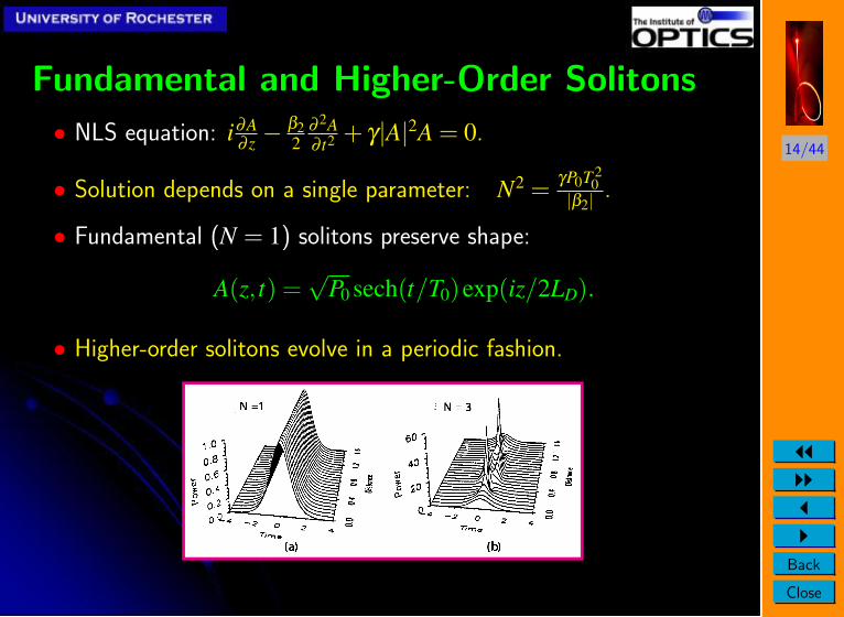
Fundamental and Higher-Order Solitons

• NLS equation: i∂A∂ z −

β22

∂ 2A∂ t2 + γ|A|2A = 0.

• Solution depends on a single parameter: N2 = γP0T 20

|β2|.

• Fundamental (N = 1) solitons preserve shape:

A(z, t) =√

P0 sech(t/T0)exp(iz/2LD).

• Higher-order solitons evolve in a periodic fashion.

15/44

JJIIJI

Back

Close

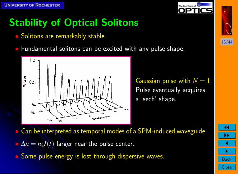
Stability of Optical Solitons• Solitons are remarkably stable.

• Fundamental solitons can be excited with any pulse shape.

Gaussian pulse with N = 1.

Pulse eventually acquires

a ‘sech’ shape.

• Can be interpreted as temporal modes of a SPM-induced waveguide.

• ∆n = n2I(t) larger near the pulse center.

• Some pulse energy is lost through dispersive waves.

16/44

JJIIJI

Back

Close

Cross-Phase Modulation

• Consider two optical fields propagating simultaneously.

• Nonlinear refractive index seen by one wave depends on the

intensity of the other wave as

∆nNL = n2(|A1|2 +b|A2|2).

• Total nonlinear phase shift:

φNL = (2πL/λ )n2[I1(t)+bI2(t)].

• An optical beam modifies not only its own phase but also of other

copropagating beams (XPM).

• XPM induces nonlinear coupling among overlapping optical pulses.

17/44

JJIIJI

Back

Close

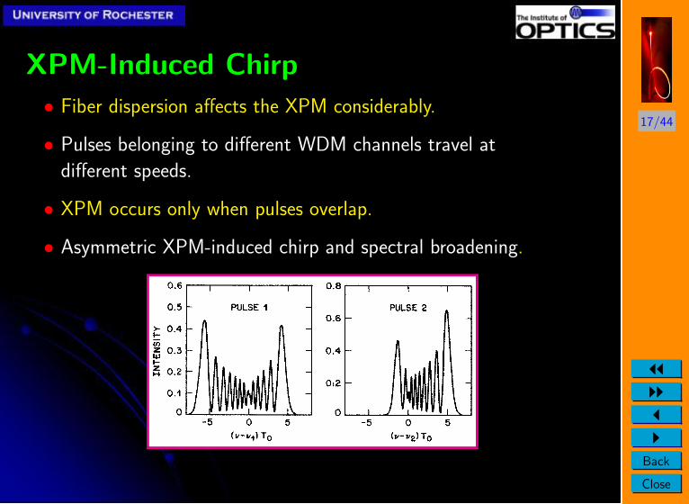
XPM-Induced Chirp

• Fiber dispersion affects the XPM considerably.

• Pulses belonging to different WDM channels travel at

different speeds.

• XPM occurs only when pulses overlap.

• Asymmetric XPM-induced chirp and spectral broadening.

18/44

JJIIJI

Back

Close

XPM: Good or Bad?

• XPM leads to interchannel crosstalk in WDM systems.

• It can produce amplitude and timing jitter.

On the other hand . . .

XPM can be used beneficially for

• Nonlinear Pulse Compression

• Passive mode locking

• Ultrafast optical switching

• Demultiplexing of OTDM channels

• Wavelength conversion of WDM channels

19/44

JJIIJI

Back

Close

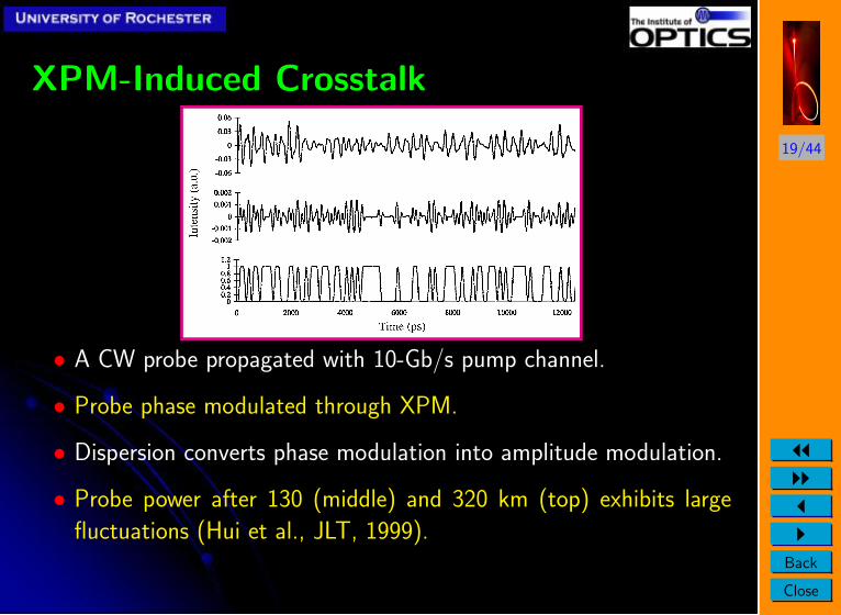
XPM-Induced Crosstalk

• A CW probe propagated with 10-Gb/s pump channel.

• Probe phase modulated through XPM.

• Dispersion converts phase modulation into amplitude modulation.

• Probe power after 130 (middle) and 320 km (top) exhibits large

fluctuations (Hui et al., JLT, 1999).

20/44

JJIIJI

Back

Close

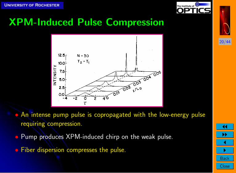
XPM-Induced Pulse Compression

• An intense pump pulse is copropagated with the low-energy pulse

requiring compression.

• Pump produces XPM-induced chirp on the weak pulse.

• Fiber dispersion compresses the pulse.

21/44

JJIIJI

Back

Close

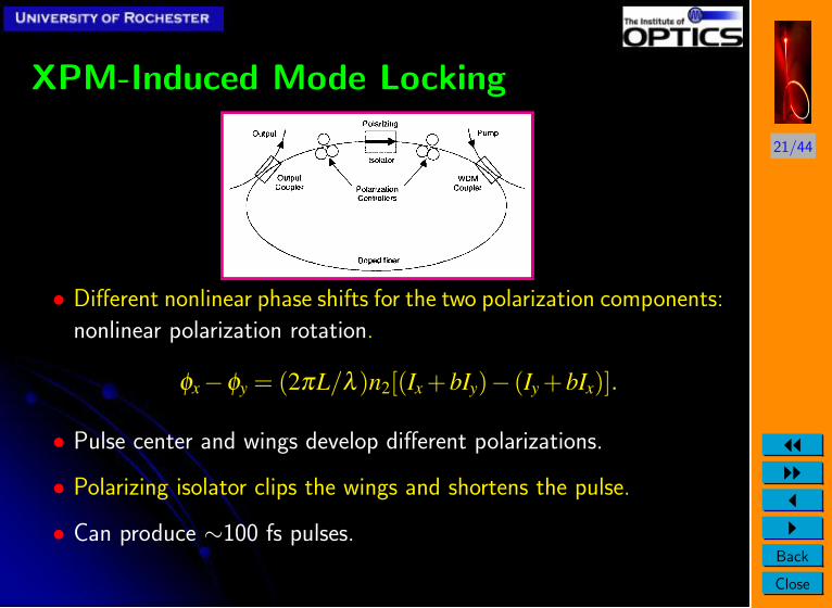
XPM-Induced Mode Locking

• Different nonlinear phase shifts for the two polarization components:

nonlinear polarization rotation.

φx−φy = (2πL/λ )n2[(Ix +bIy)− (Iy +bIx)].

• Pulse center and wings develop different polarizations.

• Polarizing isolator clips the wings and shortens the pulse.

• Can produce ∼100 fs pulses.

22/44

JJIIJI

Back

Close

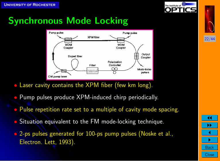
Synchronous Mode Locking

• Laser cavity contains the XPM fiber (few km long).

• Pump pulses produce XPM-induced chirp periodically.

• Pulse repetition rate set to a multiple of cavity mode spacing.

• Situation equivalent to the FM mode-locking technique.

• 2-ps pulses generated for 100-ps pump pulses (Noske et al.,

Electron. Lett, 1993).

23/44

JJIIJI

Back

Close

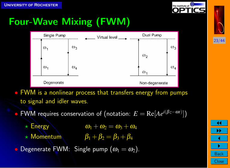
Four-Wave Mixing (FWM)

• FWM is a nonlinear process that transfers energy from pumps

to signal and idler waves.

• FWM requires conservation of (notation: E = Re[Aei(β z−ωt)])

? Energy ω1 +ω2 = ω3 +ω4

? Momentum β1 +β2 = β3 +β4

• Degenerate FWM: Single pump (ω1 = ω2).

24/44

JJIIJI

Back

Close

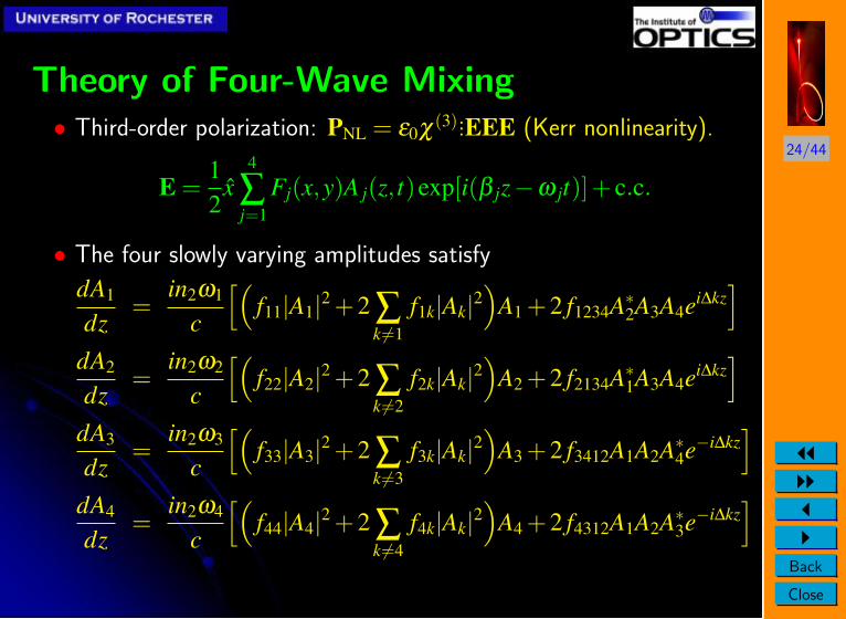
Theory of Four-Wave Mixing• Third-order polarization: PNL = ε0χ (3)...EEE (Kerr nonlinearity).

E =12

x4

∑j=1

Fj(x,y)A j(z, t)exp[i(β jz−ω jt)]+ c.c.

• The four slowly varying amplitudes satisfy

dA1

dz=

in2ω1

c

[(f11|A1|2 +2 ∑

k 6=1f1k|Ak|2

)A1 +2 f1234A∗2A3A4ei∆kz

]dA2

dz=

in2ω2

c

[(f22|A2|2 +2 ∑

k 6=2f2k|Ak|2

)A2 +2 f2134A∗1A3A4ei∆kz

]dA3

dz=

in2ω3

c

[(f33|A3|2 +2 ∑

k 6=3f3k|Ak|2

)A3 +2 f3412A1A2A∗4e−i∆kz

]dA4

dz=

in2ω4

c

[(f44|A4|2 +2 ∑

k 6=4f4k|Ak|2

)A4 +2 f4312A1A2A∗3e−i∆kz

]

25/44

JJIIJI

Back

Close

Simplified Scalar Theory• Linear phase mismatch: ∆k = β3 +β4−β1−β2.

• Overlap integrals fi jkl ≈ fi j ≈ 1/Aeff in single-mode fibers.

• Full problem quite complicated (4 coupled nonlinear equations)

• Undepleted-pump approximation =⇒ two linear coupled equations:

• Using A j = B j exp[2iγ(P1 +P2)z], the signal and idler satisfy:

dB3

dz= 2iγ

√P1 P2B∗4e−iκz,

dB4

dz= 2iγ

√P1 P2B∗3e−iκz.

• Total phase mismatch: κ = β3 +β4−β1−β2 + γ(P1 +P2).

• Nonlinear parameter: γ = n2ω0/(cAeff)∼ 10 W−1/km.

• Signal power P3 and Idler power P4 are much smaller than

pump powers P1 and P2 (Pn = |An|2 = |Bn|2).

26/44

JJIIJI

Back

Close

General Solution

• Signal and idler fields satisfy:

dB3

dz= 2iγ

√P1 P2B∗4e−iκz,

dB∗4dz

=−2iγ√

P1 P2B3eiκz.

• General solution when both the signal and idler are present at z = 0:

B3(z) = B3(0)[cosh(gz) + (iκ/2g)sinh(gz)]+ (iγ/g)

√P1P2B∗4(0)sinh(gz)e−iκz/2

B∗4(z) = B∗4(0)[cosh(gz) − (iκ/2g)sinh(gz)]− (iγ/g)

√P1P2B3(0)sinh(gz)eiκz/2

• If an idler is not launched at z = 0 (phase-insensitive amplification):

B3(z) = B3(0)[cosh(gz)+(iκ/2g)sinh(gz)]e−iκz/2

B∗4(z) = B3(0)(−iγ/g)√

P1P2 sinh(gz)eiκz/2

27/44

JJIIJI

Back

Close

Gain Spectrum

• Signal amplification factor for a FOPA:

G(ω) =P3(L,ω)P3(0,ω)

=[

1+(

1+κ2(ω)4g2(ω)

)sinh2[g(ω)L]

].

• Parametric gain: g(ω) =√

4γ2P1P2−κ2(ω)/4.

• Wavelength conversion efficiency:

ηc(ω) =P4(L,ω)P3(0,ω)

=(

1+κ2(ω)4g2(ω)

)sinh2[g(ω)L].

• Best performance for perfect phase matching (κ = 0):

G(ω) = cosh2[g(ω)L], ηc(ω) = sinh2[g(ω)L].

28/44

JJIIJI

Back

Close

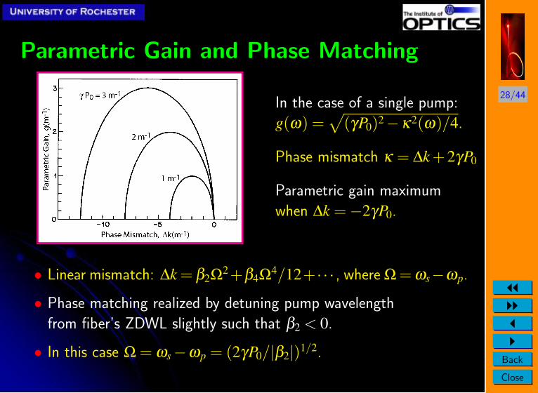
Parametric Gain and Phase Matching

In the case of a single pump:

g(ω) =√

(γP0)2−κ2(ω)/4.

Phase mismatch κ = ∆k +2γP0

Parametric gain maximum

when ∆k =−2γP0.

• Linear mismatch: ∆k = β2Ω2+β4Ω4/12+ · · · , where Ω = ωs−ωp.

• Phase matching realized by detuning pump wavelength

from fiber’s ZDWL slightly such that β2 < 0.

• In this case Ω = ωs−ωp = (2γP0/|β2|)1/2.

29/44

JJIIJI

Back

Close

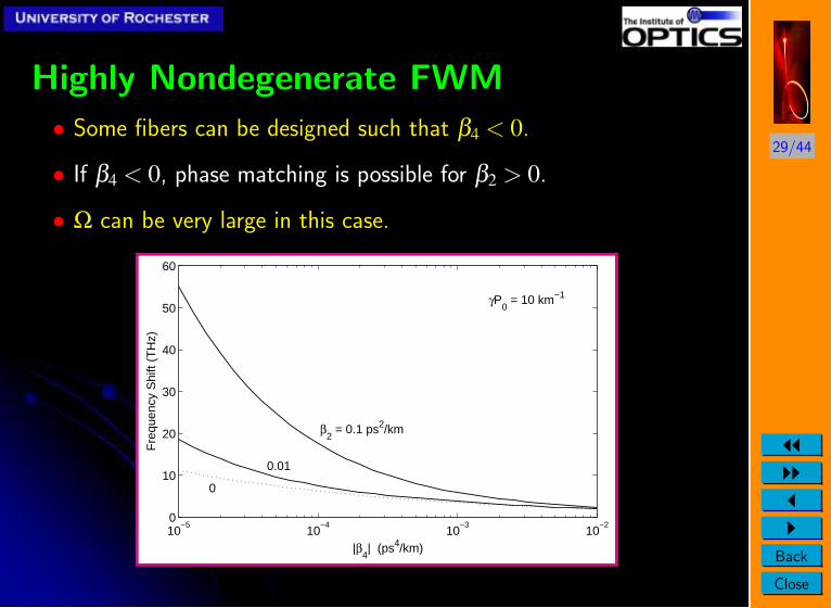
Highly Nondegenerate FWM

• Some fibers can be designed such that β4 < 0.

• If β4 < 0, phase matching is possible for β2 > 0.

• Ω can be very large in this case.

10−5

10−4

10−3

10−2

0

10

20

30

40

50

60

|β4| (ps4/km)

Fre

quen

cy S

hift

(TH

z)

β2 = 0.1 ps2/km

0.01

0

γP0 = 10 km−1

30/44

JJIIJI

Back

Close

FWM: Good or Bad?

• FWM leads to interchannel crosstalk in WDM systems.

• It generates additional noise and degrades system performance.

On the other hand . . .

FWM can be used beneficially for

• Optical amplification and wavelength conversion

• Phase conjugation and dispersion compensation

• Ultrafast optical switching and signal processing

• Generation of correlated photon pairs

31/44

JJIIJI

Back

Close

Parametric Amplification

• FWM can be used to amplify a weak signal.

• Pump power is transferred to signal through FWM.

• Peak gain Gp = 14 exp(2γP0L) can exceed 20 dB for

P0 ∼ 0.5 W and L∼ 1 km.

• Parametric amplifiers can provide gain at any wavelength using

suitable pumps.

• Two pumps can be used to obtain 30–40 dB gain over

a large bandwidth (>40 nm).

• Such amplifiers are also useful for ultrafast signal processing.

• They can be used for all-optical regeneration of bit streams.

32/44

JJIIJI

Back

Close

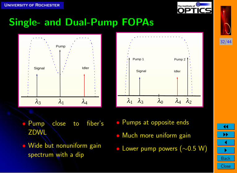
Single- and Dual-Pump FOPAs

3/30

Four-Wave Mixing (FWM)

Pump

IdlerSignal

λ3 λ1 λ4

• Pump close to fiber’s

ZDWL

• Wide but nonuniform gain

spectrum with a dip

3/31

Four-Wave Mixing (FWM)

IdlerSignal

Pump 2Pump 1

λ1 λ3 λ0 λ4 λ2

• Pumps at opposite ends

• Much more uniform gain

• Lower pump powers (∼0.5 W)

33/44

JJIIJI

Back

Close

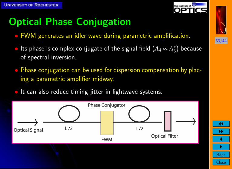
Optical Phase Conjugation

• FWM generates an idler wave during parametric amplification.

• Its phase is complex conjugate of the signal field (A4 ∝ A∗3) because

of spectral inversion.

• Phase conjugation can be used for dispersion compensation by plac-

ing a parametric amplifier midway.

• It can also reduce timing jitter in lightwave systems.

34/44

JJIIJI

Back

Close

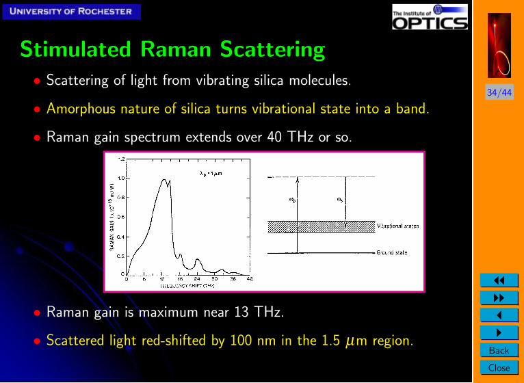
Stimulated Raman Scattering• Scattering of light from vibrating silica molecules.

• Amorphous nature of silica turns vibrational state into a band.

• Raman gain spectrum extends over 40 THz or so.

• Raman gain is maximum near 13 THz.

• Scattered light red-shifted by 100 nm in the 1.5 µm region.

35/44

JJIIJI

Back

Close

Raman Threshold• Raman threshold is defined as the input pump power at which

Stokes power becomes equal to the pump power at the fiber output:

Ps(L) = Pp(L)≡ P0 exp(−αpL).

• P0 = I0Aeff is the input pump power.

• For αs ≈ αp, threshold condition becomes

Peffs0 exp(gRP0Leff/Aeff) = P0,

• Assuming a Lorentzian shape for the Raman-gain spectrum, Raman

threshold is reached when (Smith, Appl. Opt. 11, 2489, 1972)

gRPthLeff

Aeff≈ 16 =⇒ Pth ≈

16Aeff

gRLeff.

36/44

JJIIJI

Back

Close

Estimates of Raman ThresholdTelecommunication Fibers

• For long fibers, Leff = [1− exp(−αL)]/α ≈ 1/α ≈ 20 km

for α = 0.2 dB/km at 1.55 µm.

• For telecom fibers, Aeff = 50–75 µm2.

• Threshold power Pth ∼1 W is too large to be of concern.

• Interchannel crosstalk in WDM systems because of Raman gain.

Yb-doped Fiber Lasers and Amplifiers

• Because of gain, Leff = [exp(gL)−1]/g > L.

• For fibers with a large core, Aeff ∼ 1000 µm2.

• Pth exceeds 10 kW for short fibers (L < 10 m).

• SRS may limit fiber lasers and amplifiers if L 10 m.

37/44

JJIIJI

Back

Close

SRS: Good or Bad?

• Raman gain introduces interchannel crosstalk in WDM systems.

• Crosstalk can be reduced by lowering channel powers but it limits

the number of channels.

On the other hand . . .

• Raman amplifiers are a boon for WDM systems.

• Can be used in the entire 1300–1650 nm range.

• EDFA bandwidth limited to ∼40 nm near 1550 nm.

• Distributed nature of Raman amplification lowers noise.

• Needed for opening new transmission bands in telecom systems.

38/44

JJIIJI

Back

Close

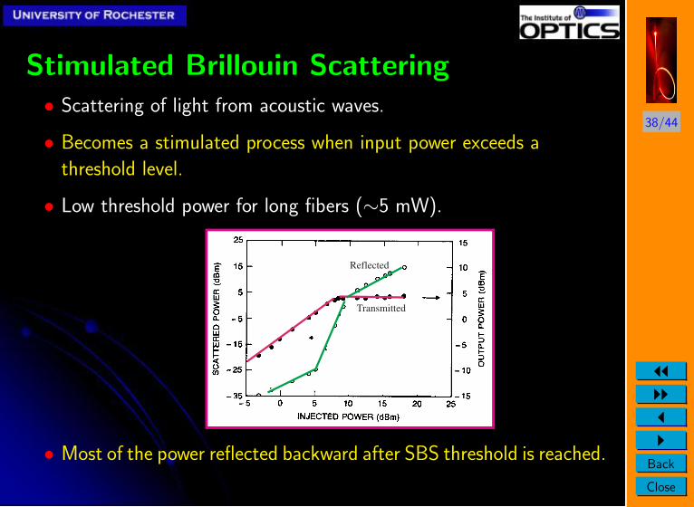
Stimulated Brillouin Scattering• Scattering of light from acoustic waves.

• Becomes a stimulated process when input power exceeds a

threshold level.

• Low threshold power for long fibers (∼5 mW).

Transmitted

Reflected

• Most of the power reflected backward after SBS threshold is reached.

39/44

JJIIJI

Back

Close

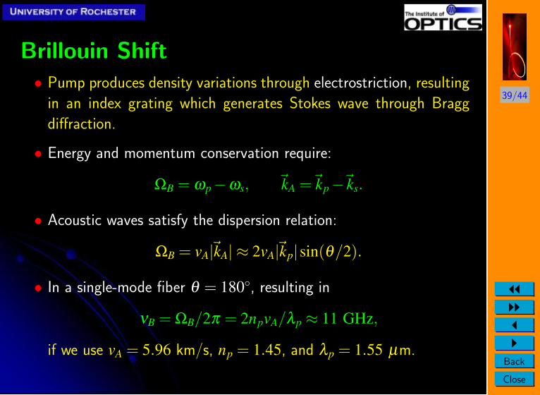
Brillouin Shift• Pump produces density variations through electrostriction, resulting

in an index grating which generates Stokes wave through Bragg

diffraction.

• Energy and momentum conservation require:

ΩB = ωp−ωs, ~kA =~kp−~ks.

• Acoustic waves satisfy the dispersion relation:

ΩB = vA|~kA| ≈ 2vA|~kp|sin(θ/2).

• In a single-mode fiber θ = 180, resulting in

νB = ΩB/2π = 2npvA/λp ≈ 11 GHz,

if we use vA = 5.96 km/s, np = 1.45, and λp = 1.55 µm.

40/44

JJIIJI

Back

Close

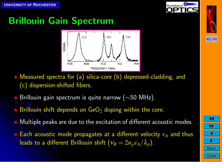
Brillouin Gain Spectrum

• Measured spectra for (a) silica-core (b) depressed-cladding, and

(c) dispersion-shifted fibers.

• Brillouin gain spectrum is quite narrow (∼50 MHz).

• Brillouin shift depends on GeO2 doping within the core.

• Multiple peaks are due to the excitation of different acoustic modes.

• Each acoustic mode propagates at a different velocity vA and thus

leads to a different Brillouin shift (νB = 2npvA/λp).

41/44

JJIIJI

Back

Close

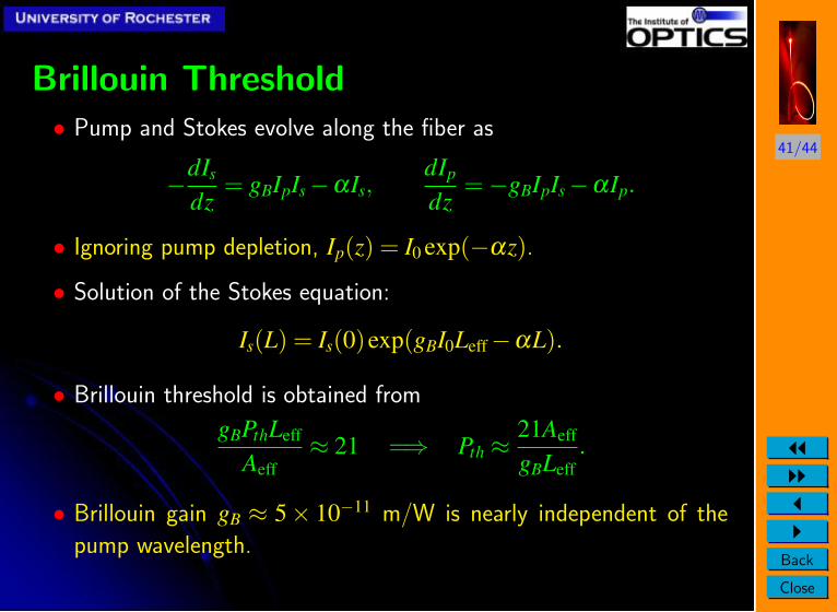
Brillouin Threshold• Pump and Stokes evolve along the fiber as

−dIs

dz= gBIpIs−αIs,

dIp

dz=−gBIpIs−αIp.

• Ignoring pump depletion, Ip(z) = I0 exp(−αz).

• Solution of the Stokes equation:

Is(L) = Is(0)exp(gBI0Leff−αL).

• Brillouin threshold is obtained from

gBPthLeff

Aeff≈ 21 =⇒ Pth ≈

21Aeff

gBLeff.

• Brillouin gain gB ≈ 5× 10−11 m/W is nearly independent of the

pump wavelength.

42/44

JJIIJI

Back

Close

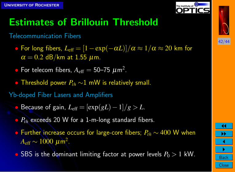
Estimates of Brillouin ThresholdTelecommunication Fibers

• For long fibers, Leff = [1− exp(−αL)]/α ≈ 1/α ≈ 20 km for

α = 0.2 dB/km at 1.55 µm.

• For telecom fibers, Aeff = 50–75 µm2.

• Threshold power Pth ∼1 mW is relatively small.

Yb-doped Fiber Lasers and Amplifiers

• Because of gain, Leff = [exp(gL)−1]/g > L.

• Pth exceeds 20 W for a 1-m-long standard fibers.

• Further increase occurs for large-core fibers; Pth ∼ 400 W when

Aeff ∼ 1000 µm2.

• SBS is the dominant limiting factor at power levels P0 > 1 kW.

43/44

JJIIJI

Back

Close

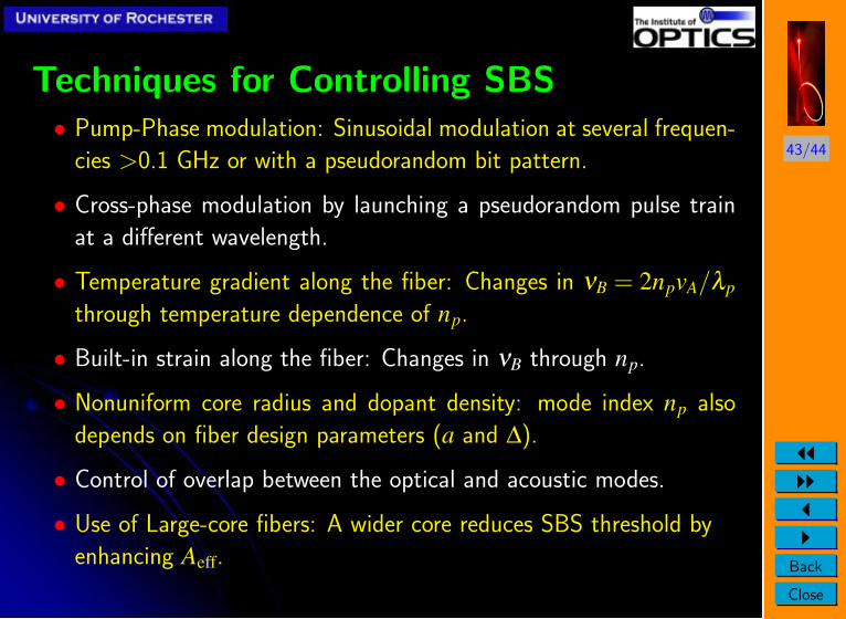
Techniques for Controlling SBS• Pump-Phase modulation: Sinusoidal modulation at several frequen-

cies >0.1 GHz or with a pseudorandom bit pattern.

• Cross-phase modulation by launching a pseudorandom pulse train

at a different wavelength.

• Temperature gradient along the fiber: Changes in νB = 2npvA/λp

through temperature dependence of np.

• Built-in strain along the fiber: Changes in νB through np.

• Nonuniform core radius and dopant density: mode index np also

depends on fiber design parameters (a and ∆).

• Control of overlap between the optical and acoustic modes.

• Use of Large-core fibers: A wider core reduces SBS threshold by

enhancing Aeff.

44/44

JJIIJI

Back

Close

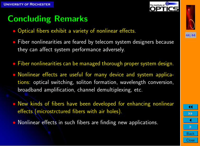
Concluding Remarks

• Optical fibers exhibit a variety of nonlinear effects.

• Fiber nonlinearities are feared by telecom system designers because

they can affect system performance adversely.

• Fiber nonlinearities can be managed thorough proper system design.

• Nonlinear effects are useful for many device and system applica-

tions: optical switching, soliton formation, wavelength conversion,

broadband amplification, channel demultiplexing, etc.

• New kinds of fibers have been developed for enhancing nonlinear

effects (microstrctured fibers with air holes).

• Nonlinear effects in such fibers are finding new applications.