Noisy Matrix Completion Using AlternatingMinimization

Suriya Gunasekar, Ayan Acharya, Neeraj Gaur, and Joydeep Ghosh

Department of ECE, University of Texas at Austin, USAsuriya@utexas.edu, aacharya@utexas.edu, neeraj.gaur@utexas.edu,

ghosh@ece.utexas.edu

Abstract. The task of matrix completion involves estimating the entries of amatrix, M ∈ Rm×n, when a subset, Ω ⊂ (i, j) : 1 ≤ i ≤ m, 1 ≤ j ≤ nof the entries are observed. A particular set of low rank models for this taskapproximate the matrix as a product of two low rank matrices, M = UV T , whereU ∈ Rm×k and V ∈ Rn×k and k minm,n. A popular algorithm of choicein practice for recovering M from the partially observed matrix using the lowrank assumption is alternating least square (ALS) minimization, which involvesoptimizing over U and V in an alternating manner to minimize the squared errorover observed entries while keeping the other factor fixed. Despite being widelyexperimented in practice, only recently were theoretical guarantees establishedbounding the error of the matrix estimated from ALS to that of the original matrixM . In this work we extend the results for a noiseless setting and provide the firstguarantees for recovery under noise for alternating minimization. We specificallyshow that for well conditioned matrices corrupted by random noise of boundedFrobenius norm, if the number of observed entries is O

(k7n logn

), then the

ALS algorithm recovers the original matrix within an error bound that dependson the norm of the noise matrix. The sample complexity is the same as derived in[7] for the noise–free matrix completion using ALS.

1 Introduction

The problem of matrix completion has found application in a number of research areassuch as in recommender systems [10], multi-task learning [15], remote sensing[12] andimage inpainting [1]. In a typical setting for matrix completion, a matrix M ∈ Rm×nis observed on a subset of entries Ω ⊂ (i, j) : 1 ≤ i ≤ m, 1 ≤ j ≤ n, while alarge number of entries are missing. The task is then to fill in the missing entries ofthe matrix yielding an estimate M of the complete matrix that is consistent with theoriginal matrix M .

Among the many models that try and tackle the matrix completion problem, lowrank models have enjoyed a great deal of success in practice and have proven to be verypopular and effective for the matrix completion task on real life datasets [3,8,10,13,11].Low rank models with numerous variations have been heavily used in practice formatrix completion specially towards the application of collaborative filtering [10,13].Though it is one of the most widely used techniques to model incomplete matrix data,there are only a few algorithms for which theoretical guarantees have been established,

2 Gunasekar et al

most notably the nuclear norm minimization [3,4] and OptSpace [8]. However, thesealgorithms are computationally expensive and hence not scalable.

A popular algorithm that is heavily used in practice for recovering M from theentries observed on Ω under the low rank assumption is the alternating least squaresminimization (ALS) [16,10]. The algorithm makes the assumption that the matrix M isof a fixed low rank that has a latent factor representationM = UV T , whereU ∈ Rm×k,V ∈ Rn×k and k n,m. Hence, one is interested in solving the following:

minU,V‖PΩ(M)− PΩ(UV T )‖2F

Where Ω is the set of observed entries and PΩ(M), also denoted by MΩ , is the projec-

tion of the matrix M onto the observed set Ω, given by, MΩij =

Mij if (i, j) ∈ Ω0 otherwise

The above problem as described is jointly non–convex in U and V . Alternating min-imization proceeds by alternatively fixing one of the latent factors and optimizing theother. Once one of the factors (say U ) is fixed, solving for the other (V ) is a convexproblem. In fact, it is a simple least squares problem. This simplicity of the alternatingminimization has made it a popular approach for low rank matrix factorization in prac-tice. Recent results [7,6,14] give recovery guarantees for ALS in a noiseless setting.However theoretical guarantees for ALS when the observed entries are corrupted bynoise are still lacking. On the other hand, in real life applications, the matrix entries areoften corrupted by various means including the noise in the matrix generation process,outliers and inaccurate measurements. In this work we present the first guarantees forrecovery under noise for alternating least squares minimization. We rely heavily on theanalysis of [7,6] and also borrow results from [9].

The paper is organized as follows. After explaining the notations and defining a fewquantities in Section 1.1, we briefly review relevant work in Section 2. In Section 3, wedescribe the algorithm and state the main result of the paper and compare the resultswith the existing results. Our primary contribution in this paper is the proof of the resultstated in Section 3. We build the proof in Section 4. As the proof is fairly involved,the proof of various lemmata in this section are deferred to the Appendix. We concludewith an analysis of the results and possible future directions in Section 5.

1.1 Notations and Preliminaries

Unless stated otherwise, we use the following notation in the rest of the paper. Matricesare represented by uppercase letters. For a matrix M , Mi represents the ith column,M (i) represents the vector corresponding to the ith row, (all the vectors are columnvectors i.e they are or dimension d × 1, where d is the length of the vector) and Mij

is the (i, j)th entry. The spectral norm and Frobenius norm of a matrix M are denotedby ‖M‖2 and ‖M‖F , respectively. The max norm of M , denoted by Mmax, is themaximum of the absolute values of the entries of M . The transpose of a matrix M isdenoted by M†. Vectors are denoted by lowercase letters. For a vector u, ui is the ithcomponent of u. The p-norm of a vector is given by ‖u‖p = (

∑i |ui|p)

1/p, p ≥ 1.Finally, set of integers from 1 to m is denoted by [m] = 1, 2, . . . ,m.

Noisy Matrix Completion Using Alternating Minimization 3

Definition 1 (SVD (or truncated SVD)). The singular value decomposition (SVD) ofa matrix M ∈ Rm×n of rank k is given by M = UΣV †, where U ∈ Rm×k andV ∈ Rn×k have orthonormal columns, i.e. U†U = V †V = I and Σ ∈ Rk×k is adiagonal matrix whose entries are (σ1, σ2, . . . , σk). Here, the columns of U and V arecalled the left and right singular vectors of M respectively and σ1 ≥ σ2, . . . , σk > 0are the singular values.

Definition 2 (Condition number). Consider a matrix M of rank k, with singular val-ues, σ1 ≥ σ2, . . . , σk > 0. The condition number of the matrix M , denoted by κM isdefined as κM = σ1

σk

Definition 3 (Reduced–QR factorization (or simply QR factorization)). The Reduced–QR factorization, which is often overloaded as QR factorization, of a matrix X ∈Rm×k, m ≥ k, is given by X = QR, where Q ∈ Rm×k has orthonormal columnsand R ∈ Rk×k is an upper triangular matrix. The columns of the matrix Q is an or-thonormal basis for the subspace spanned by the columns of X .

Definition 4 (Distance between two matrices [5]). Given two matrices U , W ∈ Rm×k,the distance between the subspaces spanned by the columns of U and W is given bydist(U , W ) = ‖U†⊥W‖2 = ‖UW †⊥‖2 where U and W are orthonormal bases of thespaces span(U) and span(W ), respectively. Similarly, U⊥ and W⊥ are orthonormalbases of the spaces span(U⊥) and span(W⊥).

Definition 5 (Incoherence of a matrix). A matrix M ∈ Rm×n is incoherent withparameter µ if ‖U (i)‖2 ≤ µ

√k√m∀i ∈ [m] and ‖V (j)‖2 ≤ µ

√k√n∀j ∈ [n] where

M = UΣV † is the SVD of M . We remind that X(i) is the ith row of matrix X .

Definition 6 (Vector to matrix conversion). The operator vec2mat() converts a vector

to matrix in column–order, i.e. ∀ x ∈ Rnk, vec2mat(x) =

↑ ↑ · · · ↑x1:n xn+1:2n · · · x(k−1)n+1:kn

↓ ↓ · · · ↓

2 Related Work

Candès and Recht [3] first demonstrated that under the assumptions of random samplingand incoherence conditions O(kn1.2 log n) samples allow for exact recovery of the trueunderlying matrix via convex nuclear–norm based minimization. The sample complex-ity result was further improved toO(kn log n) by Candès and Tao [4]. Later on, Candèsand Plan [2] analyzed the recovery guarantees for nuclear–norm based optimization al-gorithm under bounded noise added to the true underlying matrix. However, one shouldnote that nuclear–norm based minimization approach is computationally expensive andinfeasible in practice for large scale matrices.

In the OptSpace algorithm [8], Keshavan et al. adopted a different approach for thematrix completion problem where they first took the SVD of the matrix MΩ . Theiranalysis showed that such a SVD provides a reasonably good initial estimate for thespanning subspace, which can further be refined by gradient descent on a Grassmanian

4 Gunasekar et al

manifold. They show asymptotic recovery guarantees of original matrix if the number ofsamples isO(nk (σ∗1/σ

∗k)

2log n). In a later paper, Keshavan et al. [9] also examined the

reconstruction guarantee of OptSpace under two noise models. The analysis (for bothnoiseless and noisy recovery) of the algorithm only guarantees asymptotic convergenceand the convergence might take exponential time in the problem size in the worst case.

In practice, however, alternating minimization based approach produces good opti-mal solution. Though the underlying optimization problem is non–convex, each stepis convex, computationally cheaper and solutions close to global optimal are oftenreported in experiments [11]. The algorithm and its variations have been practicallydeployed in many real life collaborative filtering datasets and have shown good per-formance [10,13]. Wang and Xu [14] first showed that given a factorization algorithmattains a global optimum, the space of the factors, U and V , and the estimated matrixM are robust against corruption of the observed entries by bounded noise. Jain et al.[7,6], however, were the first to formulate the conditions for recovery of the underly-ing matrix using alternating minimization. They showed that the true underlying matrixM can be recovered within an error of ε in O(log(‖M‖F /ε)) steps and this requiresO((σ∗1/σ

∗k)

4k7n log n log ‖M‖F /ε) number of samples. We build on the results of Jainet al. [7] and provide recovery guarantees of noisy matrix completion problem withalternating minimization.

3 Main Result

In the rest of the paper, the underlying true rank–k matrix to be completed is denotedby M ∈ Rm×n. With a slight abuse of notation, the truncated SVD of M is given byM = U∗Σ∗V ∗† with U∗ ∈ Rm×k, V ∗ ∈ Rn×k and Σ∗ = diag(σ∗1 , σ

∗2 , . . . , σ

∗k).

Without loss of generality, it is assumed that m ≤ n and α = n/m ≥ 1 is a constant(independent of n). The noisy matrix which is partially observed is given by M =M+N , where N ∈ Rm×n is the noise matrix. Further, let N = UNΣNV

†N be the SVD of

the noise matrix with UN ∈ Rm×m, VN ∈ Rn×m and ΣN = diag(σN1 , σN2 , . . . , σ

Nm).

Each entry of the matrix M is independently observed with probability p. Let Ω be theset of indices where the matrix M is observed. The task is to estimate M given MΩ

and Ω.

3.1 Noise Model

We consider a fairly general, worst case model for the noise matrix N , also used in [9].In this modelN is distributed arbitrarily but bounded as |Nij | ≤ Nmax. This is a genericsetting, and any noise distribution with sub Gaussian tails can be approximated by thismodel with high probability. However, tighter bounds can be obtained for individualcases. Our bounds primarily depend on Nmax and the fractional operator norm of NΩ ,‖NΩ‖2/p. We use the following result from [9]:

Theorem 1 ([9]). If N is a matrix from the worst case model, then for any realizationof N , ‖NΩ‖2 ≤ 2|Ω|

m√αNmax.

Noisy Matrix Completion Using Alternating Minimization 5

Using, |Ω| ≈ pmn in Theorem 1, we have the following bound:

‖NΩ‖2p

≤ 2√mnNmax, (1)

3.2 Algorithm

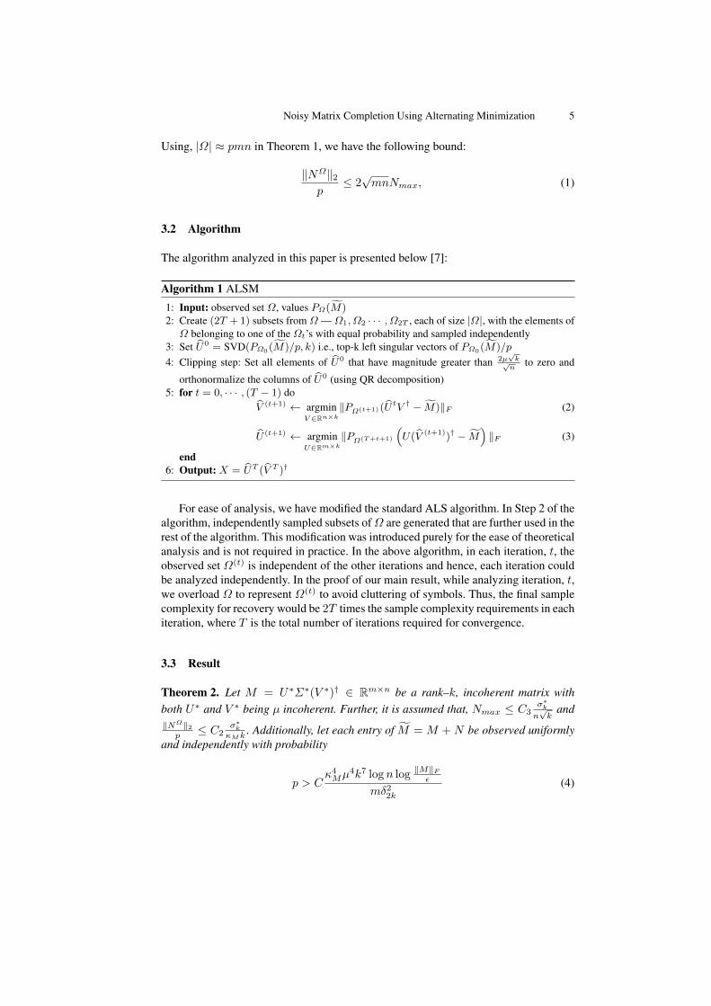
The algorithm analyzed in this paper is presented below [7]:

Algorithm 1 ALSM

1: Input: observed set Ω, values PΩ(M)2: Create (2T +1) subsets from Ω — Ω1, Ω2 · · · , Ω2T , each of size |Ω|, with the elements ofΩ belonging to one of the Ωt’s with equal probability and sampled independently

3: Set U0 = SVD(PΩ0(M)/p, k) i.e., top-k left singular vectors of PΩ0(M)/p

4: Clipping step: Set all elements of U0 that have magnitude greater than 2µ√k√n

to zero and

orthonormalize the columns of U0 (using QR decomposition)5: for t = 0, · · · , (T − 1) do

V (t+1) ← argminV ∈Rn×k

‖PΩ(t+1)(UtV † − M)‖F (2)

U (t+1) ← argminU∈Rm×k

‖PΩ(T+t+1)

(U(V (t+1))† − M

)‖F (3)

end6: Output: X = UT (V T )†

For ease of analysis, we have modified the standard ALS algorithm. In Step 2 of thealgorithm, independently sampled subsets ofΩ are generated that are further used in therest of the algorithm. This modification was introduced purely for the ease of theoreticalanalysis and is not required in practice. In the above algorithm, in each iteration, t, theobserved set Ω(t) is independent of the other iterations and hence, each iteration couldbe analyzed independently. In the proof of our main result, while analyzing iteration, t,we overload Ω to represent Ω(t) to avoid cluttering of symbols. Thus, the final samplecomplexity for recovery would be 2T times the sample complexity requirements in eachiteration, where T is the total number of iterations required for convergence.

3.3 Result

Theorem 2. Let M = U∗Σ∗(V ∗)† ∈ Rm×n be a rank–k, incoherent matrix withboth U∗ and V ∗ being µ incoherent. Further, it is assumed that, Nmax ≤ C3

σ∗kn√k

and‖NΩ‖2p ≤ C2

σ∗kκMk

. Additionally, let each entry of M = M +N be observed uniformlyand independently with probability

p > Cκ4Mµ

4k7 log n log ‖M‖Fεmδ22k

(4)

6 Gunasekar et al

where, κM =σ∗1σ∗k

is the condition number of the M , δ2k ≤ σ∗k64σ∗1

and C > 0 is a global

constant. Then with high probability, for T ≥ C ′ log ‖M‖Fε , the outputs UT and V T ofAlgorithm 1 with input (Ω,PΩ(M)) satisfy

1√mn‖M−UT (V T )†‖F ≤ ε+20µκ2Mk

1.5

(‖NΩ‖2|Ω|

)≤ ε+40µκ2Mk

1.5Nmax (5)

Worst case noise model requirements The theorem requires that Nmax ≤ C3σ∗kn√k

and ‖NΩ‖2p ≤ C2

σ∗kκMk

. For the worst case noise model, if Nmax ≤ C2σ∗k

2κMnk=⇒

‖NΩ‖2p ≤ 2

√mnNmax ≤ C2

σ∗kκMk

Further, Nmax ≤ C3σ∗k

κMnk=⇒ Nmax ≤ C3

σ∗knk ≤

C3σ∗kn√k

. Thus, choosing C = minC2/2, C3, and Nmax ≤ Cσ∗k

κMnk, both the condi-

tions on noise matrix for Theorem 2 are satisfied.For a well conditioned matrix M of condition number close to 1, the above require-

ment is approximately equivalent toNmax ≤ C ′k−1.5 ‖M‖F√mn

, which is k−1.5 fraction ofroot mean square value of the entries of matrix M . This is a fairly reasonable assump-tion on the noise matrix for recovery guarantees.

3.4 Comparison with Similar Results

The most relevant work for our analysis is the analysis of low rank matrix completionunder alternating minimization approach proposed by Jain et. al. [7]. They have thefollowing result for ALS under noiseless setting, N = 0:

Theorem 3 ([7]). Let M = U∗Σ∗(V ∗)† ∈ Rm×n be a rank–k, incoherent matrix withboth U∗ and V ∗ being µ incoherent. Let each entry of M be observed uniformly and

independently with probability, p > Cκ4Mµ

4k7 logn log√k‖M‖2ε

mδ22kwhere, δ2k ≤ σ∗k

64σ∗1and

C > 0 is a global constant. Then with high probability, for T ≥ C ′ log ‖M‖Fε , the out-puts UT and V T of Algorithm 1 with input (Ω,PΩ(M)) satisfy ‖M−UT (V T )†‖F ≤ ε

Even for a very general noise model, the sample complexity required for our analysis isthe same as that required by the noise–free analysis.

Next, we compare our bounds with the bounds obtained for noisy matrix completionby Keshavan et. al [9]. The algorithm suggested by Keshavan et. al., OptSpace, involvesoptimizing the initial estimate from SVD of PΩ(M) over a Grassmann manifold. Themain result in their paper is stated below:

Theorem 4 ([9]). Let M = M + N , where M is a rank–k, µ incoherent matrix. Asubset, Ω ⊂ [m]× [n], of entries of M are revealed. Let M be the output of OptSpaceon the input of (M,Ω). Then, there exists numerical constants, C and C ′ such that,if |Ω| ≥ Cn

√ακ2M maxµk

√α log n;µ2k2ακ4M and ‖N

Ω‖2p ≤ C ′

σ∗kκ2M

√k

then, with

probability atleast 1− 1/n3, 1√mn‖M − M‖F ≤ C ′κ2Mk0.5

(‖NΩ‖2|Ω|

)

Noisy Matrix Completion Using Alternating Minimization 7

The requirements on the noise matrix for recovery guarantees by OptSpace is close tothat derived in our results for Alternating minimization. Also, the error in the recoveredmatrix in our analysis is off by a small factor of k as compared to the analysis in [9].However, the sample complexity required by ALS as evaluated by our analysis is muchhigher than that of Keshavan et. al.

4 Proof of Theorem 2

In this section we present the proof of Theorem 2. The outline of the proof is as follows.In Section 4.1, Theorem 5 states that the initialization step of the Algorithm describedin 1 provides a good starting point. In Section 4.2, we first propose a modificationto the ALSM algorithm and prove that the modification in practice is equivalent to theoriginal ALSM algorithm, while the modified algorithm is easier to analyze. Theorem 6is then stated without proof. This theorem establishes that the space spanned by ALSMestimates of U and V converge towards U∗ and V ∗ respectively. Finally, we combinethe results on initialization and above mentioned theorem to prove the main result. Theproof of Theorem 6 is deferred to Section 4.3. In each subsection, the relevant lemmataare first presented and then the main theorems are proved. The proofs of the lemmataare provided in the Appendix.

4.1 InitializationLemma 1 (Theorem 1.1 of [8]). Let M = M + N be such that M is rank–k andµ–incoherent and |Ω| ≥ Cnkmaxlog n, k. Further, from the SVD of M

Ω

p , we get a

rank–k approximation as, MΩk = U0Σ0V 0†, where U0 ∈ Rm×k and V 0 ∈ Rn×k. Let

α = n/m ≥ 1. Then the following is true with probability greater than (1− 1/n3),

1√mn‖M − MΩ

k ‖2 ≤ CMmax

(mα3/2

|Ω|

)1/2

+2m√α

|Ω|‖NΩ‖2. (6)

Lemma 2. Let U0 be defined as in Lemma 1. Further, under the conditions of Theorem2, the following is true with probability greater than (1− 1/n3),

dist(U0, U∗) ≤ 1

64k.

The proof of Lemma 2 is presented in Appendix B.1.

Theorem 5 (ALSM has a good initial point). Let U c be obtained from U0 definedabove, by setting all the entries greater than 2µ

√k√

mto zero. Let U0 be the orthonormal

basis of U c. Then under the conditions of Lemma 2, w.h.p. we have

– dist(U0, U∗) ≤ 1/2.– U0 is incoherent with parameter µ1 =

32σ∗1µ√k

σ∗k.

The proof follows directly from Lemma C.2 in [6] and Lemma 2. Note that the U0 defined above is the same as the the initial estimate, U0 from the

initialization step of the Algorithm 1.

8 Gunasekar et al

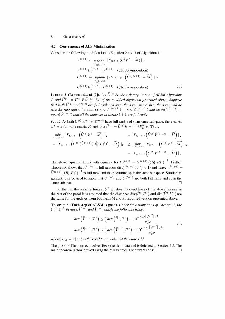
4.2 Convergence of ALS Minimization

Consider the following modification to Equation 2 and 3 of Algorithm 1:

V (t+1) ← argminV ∈Rn×k

‖PΩ(t+1)(U tV † − M)‖F

V (t+1)R(t+1)V = V (t+1) (QR decomposition)

U (t+1) ← argminU∈Rm×k

‖PΩ(T+t+1)

(UV (t+1)† − M

)‖F

U (t+1)R(t+1)U = U (t+1) (QR decomposition) (7)

Lemma 3 (Lemma 4.4 of [7]). Let U (t) be the t-th step iterate of ALSM Algorithm1, and U (t) = U (t)R

(t)U be that of the modified algorithm presented above. Suppose

that both U (t) and U (t) are full rank and span the same space, then the same will betrue for subsequent iterates. i.e span(V (t+1)) = span(V (t+1)) and span(U (t+1)) =

span(U (t+1)) and all the matrices at iterate t+ 1 are full rank.

Proof. As both U (t), U (t) ∈ Rm×k have full rank and span same subspace, there existsa k × k full rank matrix R such that U (t) = U (t)R = U (t)R

(t)U R. Thus,

minV ∈Rn×k

‖PΩ(t+1)

(U (t)V † − M

)‖2 = ‖PΩ(t+1)

(U (t)V (t+1)† − M

)‖2

= ‖PΩ(t+1)

(U (t)(V (t+1)(R

(t)U R)†)† − M

)‖2 ≥ min

V ∈Rn×k‖PΩ(t+1)

(U (t)V † − M

)‖2

= ‖PΩ(t+1)

(U (t)V (t+1)† − M

)‖2

The above equation holds with equality for V (t+1) = V (t+1)((RtUR)

†)−1. FurtherTheorem 6 shows that V (t+1) is full rank (as dist(V (t+1), V ∗) < 1) and hence, V (t+1) =

V (t+1)((RtUR)

†)−1 is full rank and their columns span the same subspace. Similar ar-guments can be used to show that U (t+1) and U (t+1) are both full rank and span thesame subspace.

Further, as the initial estimate, U0 satisfies the conditions of the above lemma, inthe rest of the proof it is assumed that the distances dist(U t, U∗) and dist(V t, V ∗) arethe same for the updates from both ALSM and its modified version presented above.

Theorem 6 (Each step of ALSM is good). Under the assumptions of Theorem 2, the(t+ 1)th iterates, U t+1 and V t+1 satisfy the following w.h.p:

dist(V t+1, V ∗

)≤ 1

4dist

(U t, U∗

)+ 10

µκM‖NΩ‖2kσ∗kp

dist(U t+1, U∗

)≤ 1

4dist

(V t+1, U∗

)+ 10

µκM‖NΩ‖2kσ∗kp

(8)

where, κM = σ∗1/σ∗k is the condition number of the matrix M .

The proof of Theorem 6, involves few other lemmata and is deferred to Section 4.3. Themain theorem is now proved using the results from Theorem 5 and 6.

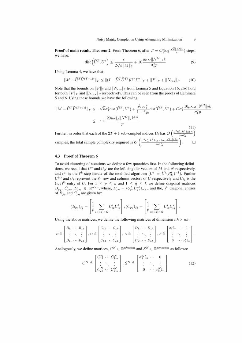
Noisy Matrix Completion Using Alternating Minimization 9

Proof of main result, Theorem 2 From Theorem 6, after T = O(log√k‖M‖2ε ) steps,

we have:

dist(UT , U∗

)≤ ε

2√k‖M‖2

+ 10µκM‖NΩ‖2k

σ∗kp(9)

Using Lemma 4, we have that:

‖M − UT V (T+1)†‖F ≤ ‖(I − UT UT†)U∗Σ∗‖F + ‖F‖F + ‖Nres‖F (10)

Note that the bounds on ‖F‖2 and ‖Nres‖2 from Lemma 5 and Equation 16, also holdfor both ‖F‖F and ‖Nres‖F respectively. This can be seen from the proofs of Lemmata5 and 6. Using these bounds we have the following:

‖M − UT V (T+1)†‖F ≤√kσ∗1dist(UT , U∗) +

δ2kσ∗1

1− δ2kdist(UT , U∗) + Cσ∗k

10µκM‖NΩ‖2kσ∗kp

≤ ε+20µκ2M‖NΩ‖2k1.5

p(11)

Further, in order that each of the 2T + 1 sub-sampled indices Ωt has O(µ4κ4

Mk7 logn

mδ22k

)samples, the total sample complexity required is O

(µ4κ4

Mk7 logn log

√k‖M‖2ε

mδ22k

).

4.3 Proof of Theorem 6

To avoid cluttering of notations we define a few quantities first. In the following defini-tions, we recall that U∗ and UN are the left singular vectors of M and N respectively,and U t is the tth step iterate of the modified algorithm (U t = U t(RtU )

−1). FurtherU (i) and Ui represent the ith row and column vectors of U respectively and Uij is the(i, j)th entry of U . For 1 ≤ p ≤ k and 1 ≤ q ≤ k we define diagonal matricesBpq, Cpq, Dpq ∈ Rn×n, where, Dpq = 〈U tp, U∗q 〉In×n and the, jth diagonal entriesof Bpq and Cpq are given by:

(Bpq)jj =

1p

∑i:(i,j)∈Ω

U tipUtiq

, (Cpq)jj =1p

∑i:(i,j)∈Ω

U tipU∗iq

.Using the above matrices, we define the following matrices of dimension nk × nk:

B ,

B11 · · · B1k

.... . .

...Bk1 · · · Bkk

, C ,C11 · · · C1k

.... . .

...Ck1 · · · Ckk

, D ,D11 · · · D1k

.... . .

...Dk1 · · · Dkk

, S ,σ∗1In · · · 0

.... . .

...0 · · · σ∗kIn

.Analogously, we define matrices, CN ∈ Rnk×nm and SN ∈ Rnm×nm as follows:

CN ,

CN11 · · · CN1m...

. . ....

CNk1 · · · CNkm

, SN ,σ

N1 In · · · 0...

. . ....

0 · · · σNmIn

(12)

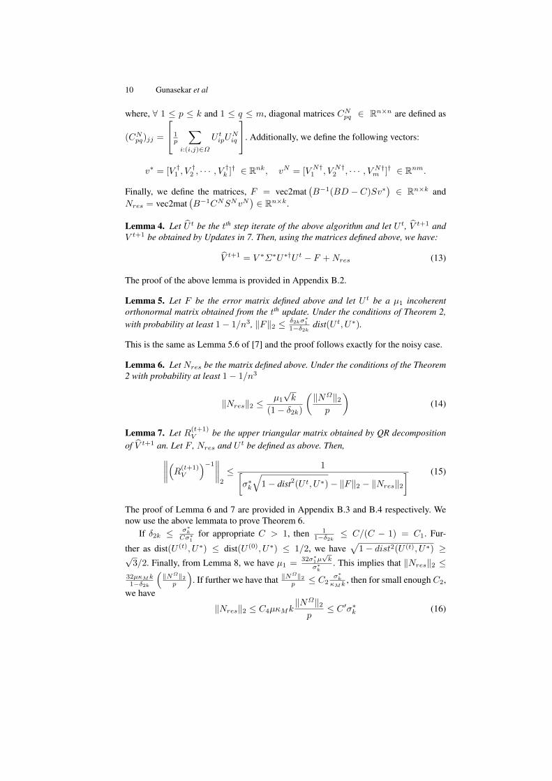
10 Gunasekar et al

where, ∀ 1 ≤ p ≤ k and 1 ≤ q ≤ m, diagonal matrices CNpq ∈ Rn×n are defined as

(CNpq)jj =

1p

∑i:(i,j)∈Ω

U tipUNiq

. Additionally, we define the following vectors:

v∗ = [V †1 , V†2 , · · · , V

†k ]† ∈ Rnk, vN = [V N†1 , V N†2 , · · · , V N†m ]† ∈ Rnm.

Finally, we define the matrices, F = vec2mat(B−1(BD − C)Sv∗

)∈ Rn×k and

Nres = vec2mat(B−1CNSNvN

)∈ Rn×k.

Lemma 4. Let U t be the tth step iterate of the above algorithm and let U t, V t+1 andV t+1 be obtained by Updates in 7. Then, using the matrices defined above, we have:

V t+1 = V ∗Σ∗U∗†U t − F +Nres (13)

The proof of the above lemma is provided in Appendix B.2.

Lemma 5. Let F be the error matrix defined above and let U t be a µ1 incoherentorthonormal matrix obtained from the tth update. Under the conditions of Theorem 2,with probability at least 1− 1/n3, ‖F‖2 ≤ δ2kσ

∗1

1−δ2k dist(U t, U∗).

This is the same as Lemma 5.6 of [7] and the proof follows exactly for the noisy case.

Lemma 6. Let Nres be the matrix defined above. Under the conditions of the Theorem2 with probability at least 1− 1/n3

‖Nres‖2 ≤µ1

√k

(1− δ2k)

(‖NΩ‖2p

)(14)

Lemma 7. Let R(t+1)V be the upper triangular matrix obtained by QR decomposition

of V t+1 an. Let F , Nres and U t be defined as above. Then,∥∥∥∥(R(t+1)V

)−1∥∥∥∥2

≤ 1[σ∗k

√1− dist2(U t, U∗)− ‖F‖2 − ‖Nres‖2

] (15)

The proof of Lemma 6 and 7 are provided in Appendix B.3 and B.4 respectively. Wenow use the above lemmata to prove Theorem 6.

If δ2k ≤ σ∗kCσ∗1

for appropriate C > 1, then 11−δ2k ≤ C/(C − 1) = C1. Fur-

ther as dist(U (t), U∗) ≤ dist(U (0), U∗) ≤ 1/2, we have√

1− dist2(U (t), U∗) ≥√3/2. Finally, from Lemma 8, we have µ1 =

32σ∗1µ√k

σ∗k. This implies that ‖Nres‖2 ≤

32µκMk1−δ2k

(‖NΩ‖2p

). If further we have that ‖N

Ω‖2p ≤ C2

σ∗kκMk

, then for small enough C2,we have

‖Nres‖2 ≤ C4µκMk‖NΩ‖2p

≤ C ′σ∗k (16)

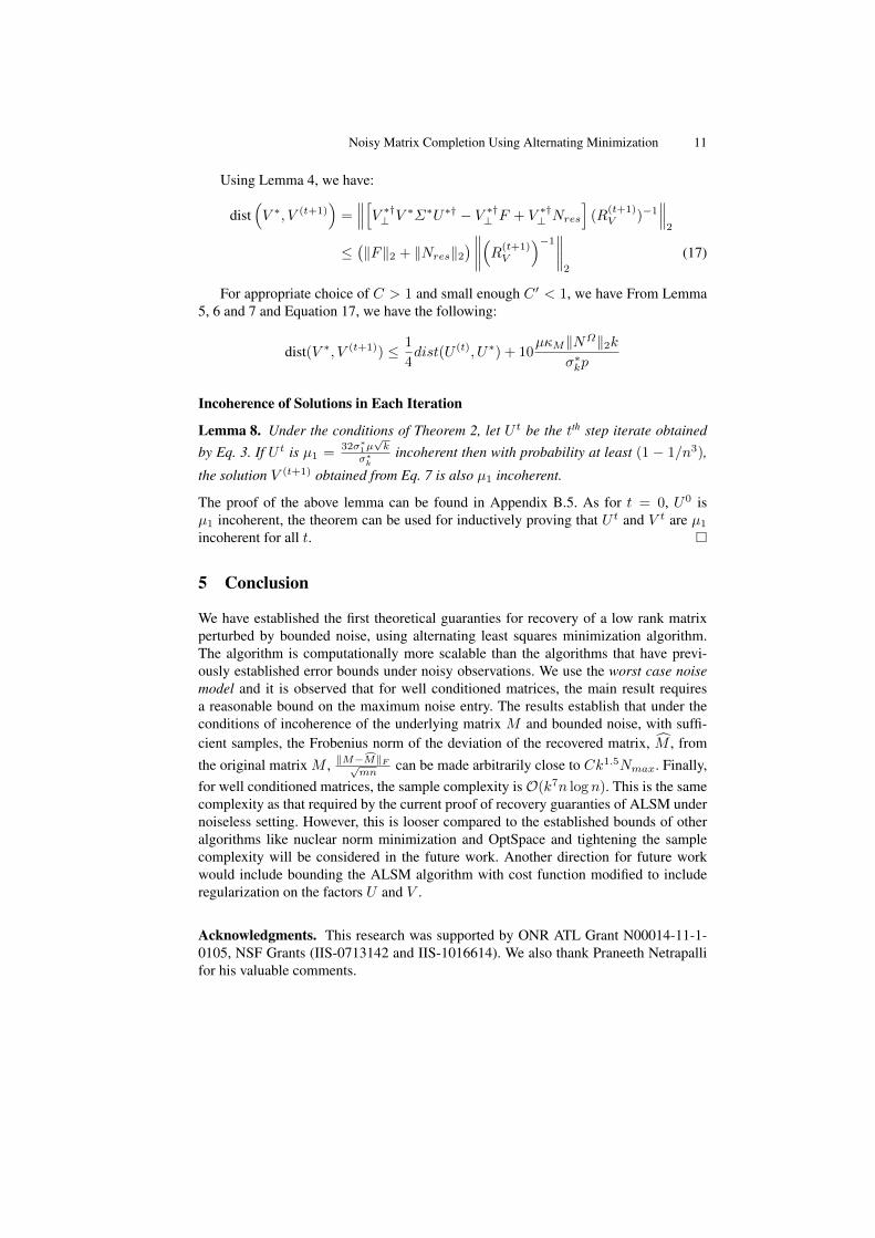
Noisy Matrix Completion Using Alternating Minimization 11

Using Lemma 4, we have:

dist(V ∗, V (t+1)

)=∥∥∥[V ∗†⊥ V ∗Σ∗U∗† − V ∗†⊥ F + V ∗†⊥ Nres

](R

(t+1)V )−1

∥∥∥2

≤(‖F‖2 + ‖Nres‖2

) ∥∥∥∥(R(t+1)V

)−1∥∥∥∥2

(17)

For appropriate choice of C > 1 and small enough C ′ < 1, we have From Lemma5, 6 and 7 and Equation 17, we have the following:

dist(V ∗, V (t+1)) ≤ 1

4dist(U (t), U∗) + 10

µκM‖NΩ‖2kσ∗kp

Incoherence of Solutions in Each Iteration

Lemma 8. Under the conditions of Theorem 2, let U t be the tth step iterate obtainedby Eq. 3. If U t is µ1 =

32σ∗1µ√k

σ∗kincoherent then with probability at least (1 − 1/n3),

the solution V (t+1) obtained from Eq. 7 is also µ1 incoherent.

The proof of the above lemma can be found in Appendix B.5. As for t = 0, U0 isµ1 incoherent, the theorem can be used for inductively proving that U t and V t are µ1

incoherent for all t.

5 Conclusion

We have established the first theoretical guaranties for recovery of a low rank matrixperturbed by bounded noise, using alternating least squares minimization algorithm.The algorithm is computationally more scalable than the algorithms that have previ-ously established error bounds under noisy observations. We use the worst case noisemodel and it is observed that for well conditioned matrices, the main result requiresa reasonable bound on the maximum noise entry. The results establish that under theconditions of incoherence of the underlying matrix M and bounded noise, with suffi-cient samples, the Frobenius norm of the deviation of the recovered matrix, M , fromthe original matrix M , ‖M−M‖F√

mncan be made arbitrarily close to Ck1.5Nmax. Finally,

for well conditioned matrices, the sample complexity isO(k7n log n). This is the samecomplexity as that required by the current proof of recovery guaranties of ALSM undernoiseless setting. However, this is looser compared to the established bounds of otheralgorithms like nuclear norm minimization and OptSpace and tightening the samplecomplexity will be considered in the future work. Another direction for future workwould include bounding the ALSM algorithm with cost function modified to includeregularization on the factors U and V .

Acknowledgments. This research was supported by ONR ATL Grant N00014-11-1-0105, NSF Grants (IIS-0713142 and IIS-1016614). We also thank Praneeth Netrapallifor his valuable comments.

12 Gunasekar et al

References1. M Bertalmio, L Vese, G Sapiro, and S Osher. Simultaneous structure and texture image

inpainting. IEEE Transactions on Image Processing, 2003.2. E. J. Candès and Y. Plan. Matrix completion with noise. CoRR, 2009.3. E. J. Candès and B. Recht. Exact matrix completion via convex optimization. Foundations

of Computational Mathematics, 2009.4. E. J. Candès and T. Tao. The power of convex relaxation: near-optimal matrix completion.

IEEE Transactions on Information Theory, 2010.5. G. H. Golub and C. F. van Van Loan. Matrix Computations (Johns Hopkins Studies in

Mathematical Sciences)(3rd Edition). The Johns Hopkins University Press, 1996.6. P. Jain, P. Netrapalli, and S. Sanghavi. Low-rank matrix completion using alternating mini-

mization. ArXiv e-prints, December 2012.7. P. Jain, P. Netrapalli, and S. Sanghavi. Low-rank matrix completion using alternating mini-

mization. In STOC, 2013.8. R. H. Keshavan, A. Montanari, and S. Oh. Matrix completion from a few entries. IEEE

Transactions on Information Theory, 2010.9. R. H. Keshavan, A. Montanari, and S. Oh. Matrix completion from noisy entries. JMLR,

2010.10. Y. Koren, R. Bell, and C. Volinsky. Matrix factorization techniques for recommender sys-

tems. IEEE Computer, 2009.11. K. Mitra, S. Sheorey, and R. Chellappa. Large-scale matrix factorization with missing data

under additional constraints. In NIPS, 2010.12. A. M. C. So and Y. Ye. Theory of semidefinite programming for sensor network localization.

In ACM-SIAM symposium on Discrete algorithms, 2005.13. G. Takács, I. Pilászy, B. Németh, and D. Tikk. Investigation of various matrix factorization

methods for large recommender systems. In KDD Workshop on Large-Scale RecommenderSystems and the Netflix Prize Competition, 2008.

14. Y. Wang and H. Xu. Stability of matrix factorization for collaborative filtering. In ICML,2012.

15. K. Yu and V. Tresp. Learning to learn and collaborative filtering. In NIPS Workshop onInductive Transfer: 10 Years Later, 2005.

16. Y. Zhou, D. Wilkinson, R. Schreiber, and R. Pan. Large-scale parallel collaborative filter-ing for the netflix prize. In Proc. 4th IntŠl Conf. Algorithmic Aspects in Information andManagement, LNCS 5034, 2008.

Appendix A

– ‖M‖2 ≤ ‖M‖F ≤√k‖M‖2

– If a matrix M is µ-incoherent, then,

Mmax ≤µ2√k√

mn‖M‖F ≤

µ2k√mn‖M‖2 (18)

– Bernstein’s Inequality: LetXi, i = 1, 2, . . . , n be independent random numbers.Let |Xi| ≤ L ∀ i w.p. 1. Then we have the following inequalities:

P [∑ni=1Xi −

∑ni=1 E[Xi] > t] ≤ exp

(−t2/2∑n

i=1 V ar(Xi)+Lt/3

)P [∑ni=1Xi −

∑ni=1 E[Xi] < −t] ≤ exp

(−t2/2∑n

i=1 V ar(Xi)+Lt/3

)(19)

Noisy Matrix Completion Using Alternating Minimization 13

Appendix B

B.1 Initialization Proofs

Proof (Proof of Lemma 2).

‖M − MΩk ‖22 = ‖U∗Σ∗V ∗† − U0Σ0V 0†‖22

= ‖(I − U0U0†)U∗Σ∗V ∗† + U0(U0†U∗Σ∗V ∗† − Σ0V 0†)‖22(1)= ‖(I − U0U0†)U∗Σ∗V ∗†‖22 + ‖U0(U0†U∗Σ∗V ∗† −ΣV †)‖22≥ ‖(I − U0U0†)U∗Σ∗V ∗†‖22 = ‖U0†

⊥ U∗Σ∗‖22 ≥ σ∗2k ‖U

0†⊥ U

∗‖22where, (1) follows as the two terms span orthogonal spaces. Hence,

dist(U0, U∗) ≤ 1

σ∗k‖M − MΩ

k ‖2(2)

≤ 1

σ∗k

CMmax

√mα3/2

p+ 2‖NΩ‖2p

(3)

≤ Cµ2kσ∗1σ∗k

√mα3/2

pmn+

2‖NΩ‖2pσ∗k

≤ 1

64k, if p >

C ′k4µ4σ∗21mσ∗2k

and‖NΩ‖2p

≤ C ′′σ∗k

k.

where, (2) follows from Lemma 1 and (3) follows from Equation 18

B.2 Proof of Lemma 4

We recall that M (i) is the ith row of the matrix M . Given, U t, the tth step iterate. Theupdate of V (t+1) is guided by the following equation from 7.

V (t+1) = argminV ∈Rn×k

‖PΩ(U tV †)− PΩ(M)‖2F

= argminV ∈Rn×k

∑(i,j)∈Ω

(U t(i)†V (j) − U∗(i)†Σ∗V ∗(j) − U (i)†

N ΣNV(j)N

)2Taking the gradient with respect to each V (j) and setting it to 0 for the optimum

V = V (t+1), we have the following ∀ j ∈ [n]:∑i:(i,j)∈Ω

U t(i)(U t(i)†

(V (t+1)

)(j)− U∗(i)†Σ∗V ∗(j) − U (i)†

N ΣNV(j)N

)= 0 (20)

We further define matrices Bj , Cj , Dj ∈ Rk×k and CjN ∈ Rk×m for 1 ≤ j ≤ n asfollows:

Bj =1

p

∑i:(i,j)∈Ω

U t(i)U t(i)†, Cj =1

p

∑i:(i,j)∈Ω

U t(i)U∗(i)†,

Dj = U t†U∗, CjN =1

p

∑i:(i,j)∈Ω

U t(i)UN(i)†. (21)

14 Gunasekar et al

It is useful to note that Bj ∈ Rk×k is obtained by taking the jth diagonal elementsof Bpq (defined in Equation 12), for 1 ≤ p, q ≤ k, i.e. (Bj)pq = (Bpq)jj . The othermatrices are defined similarly. Using the above matrices, we have from the previousequation:(V (t+1)

)(j)= DjΣ∗V ∗(j) − (Bj)−1

(BjDj − Cj

)Σ∗V ∗(j) + (Bj)−1CjNΣNV

(j)N

V (t+1) = V ∗Σ∗U∗†U t − F +Nres(22)

The last equation above can be easily seen by writing the structure of matrices definedabove.

B.3 Proof of Lemma 6From Lemma C.6 of [6], under the assumptions on p andM specified in the Lemma, wehave, ‖B−1‖2 ≤ 1

1−δ2k . Further from the structure of the matrices CN , SN and CjN , it

can be verified that ‖CNSNvN‖22 =

n∑j=1

‖C(j)N ΣNV

(j)N ‖

22. Recall that V (j)

N ∈ Rm×1 is

the jth row of VN ∈ Rn×m (a similar decomposition is used in Equation 22). Thus wehave:

∥∥CNSNvN∥∥22=

n∑j=1

∥∥∥C(j)ΣNV(j)N

∥∥∥22=

n∑j=1

∥∥∥∥∥∥1p∑

i:(i,j)∈Ω

U t(i)U(i)†N ΣNV

(j)N

∥∥∥∥∥∥2

2

≤ 1

p2

n∑j=1

∑i:(i,j)∈Ω

‖U t(i)Nij‖22 ≤1

p2

∑(i,j)∈Ω

‖U t(i)‖22|Nij |22

≤ µ21k

(‖NΩ‖F√

mp

)2

≤ µ21k

(‖NΩ‖2p

)2

(23)

This implies that

‖Nres‖2 ≤ ‖Nres‖F = ‖B−1CNSNvN‖2 ≤ ‖B−1‖2‖CNSNvN‖2 (24)

≤ µ1

√k

(1− δ2k)

(‖NΩ‖2p

).

B.4 Proof of Lemma 7

1

‖(R(t+1)V )−1‖2

= σmin(R(t+1)V ) = min

z:‖z‖2=1‖R(t+1)

V z‖2 = minz:‖z‖2=1

‖V (t+1)R(t+1)V z‖2

= minz:‖z‖2=1

‖V (t+1)z‖2 = minz:‖z‖2=1

‖(V ∗Σ∗(U∗)†U t − F +Nres

)z‖2

≥ minz:‖z‖2=1

[‖V ∗Σ∗(U∗)†U tz‖2 − ‖F‖2 − ‖Nres‖2

]≥ σ∗k min

z:‖z‖2=1‖(U∗)†U tz‖2 − ‖F‖2 − ‖Nres‖2

= σ∗k√1− dist(U t, U∗)2 − ‖F‖2 − ‖Nres‖2

Noisy Matrix Completion Using Alternating Minimization 15

Thus, ‖(R(t+1)V )−1‖2 ≤ 1

σ∗k

√1−dist(Ut,U∗)2−‖F‖2−‖Nres‖2

B.5 Proof of Lemma 8

In this proof, we use the following set of inequalities:

‖(Bj)−1‖2 ≤1

1 + δ2k

‖Bj‖2 ≤ 1 + δ2k, ‖Cj‖2 ≤ 1 + δ2k, ‖Dj‖ ≤ ‖U∗‖2‖U t‖2 = 1.

(25)

The above set of equations involve terms that does not depend on the noise and henceare incorporated from Appendix C.3 of [7]. It can be verified that the proof does notchange for the noisy case. We omit the derivation here to avoid redundancy.

Lemma 9. Under the conditions of Theorem 2, w.p. greater that 1− 1/n3

‖CjNΣNV(j)N ‖2 ≤ Nmaxµ1

√km(1 + δ2k)

We prove the above lemma at the end of this section. Now, from Equation 22, we have:(V (t+1)

)(j)= DjΣ∗V ∗(j) − (Bj)−1

(BjDj − Cj

)Σ∗V ∗(j) + (Bj)−1CjNΣNV

∗(j)N

Thus,∥∥∥∥(V (t+1))(j)∥∥∥∥

2

≤ ‖(R(t+1))−1‖2[(‖Dj‖2 + ‖(Bj)−1‖2(‖BjDj‖2 + ‖Cj‖2)

)‖Σ∗‖‖V ∗(j)‖2

+ ‖(Bj)−1‖2‖CjNΣNV∗(j)N ‖2

](26)

Using equations from 25, Lemma 9 and 7, and δ2k ≤ 1C , C > 1 we have the following:∥∥∥∥(V (t+1)

)(j)∥∥∥∥2

≤ ‖(R(t+1))−1‖2

[σ∗1µ√k√

n

(1 +

(2(1 + δ2k))

1− δ2k

)+Nmaxµ1

√km(1 + δ2k)

1− δ2k

]

= ‖(R(t+1))−1‖2

[4σ∗1µ

√k√

n+ 2Nmaxµ1

√km

](27)

We now use that for, µ1 =32µσ∗1

√k

σ∗kand further, Nmax ≤ C3

σ∗kn√k

. Choosing C3 ap-

propriately, we have Nmaxµ1

√km ≤ 2σ∗1µ

√k√

n. Finally, using Lemmata 5 and 6, the

fact that dist(U∗, U t) ≤ dist(U∗, U0) ≤ 0.5 and using the conditions on ‖NΩ‖2 fromTheorem 2 , we have, ‖(R(t+1))−1‖2 ≤ 4

σ∗k. Using these we have:∥∥∥∥(V (t+1)

)(j)∥∥∥∥2

≤ ‖(R(t+1))−1‖28σ∗1µ

√k√

n≤ 32σ∗1µ

√k

σ∗k√n

(28)

Thus we have, µ(V (t+1)) ≤ 32σ∗1µσ∗k≤ 32σ∗1µ

√k

σ∗k.

16 Gunasekar et al

Proof of Lemma 9 ‖CjNΣNV(j)N ‖2 = maxx:‖x‖2=1 x

†CjNΣNV(j)N . Given any x such

that ‖x‖2 = 1, then

x†CjNΣNV(j)N =

1

p

∑i:(i,j)∈Ω

x†U t(i)U(i)†N ΣNV

(j)N =

1

p

∑i:(i,j)∈Ω

x†U t(i)Nij (29)

We define δij =1 if (i, j) ∈ Ω0 otherwise , Zi = 1

pδijx†U t(i)Nij and Z =

∑mi=1 Zi

E[Z] =

m∑i=1

E[Zi] =

m∑i=1

x†U t(i)Nij ≤ Nmaxm∑i=1

‖U t(i)‖2 = Nmaxµ1

√km (30)

var(Z) =

m∑i=1

E[Z2i ]− (E[Zi])

2 =1− pp

m∑i=1

(x†U t(i)

)2N2ij

≤ 1

pN2max

m∑i=1

‖U t(i)‖22 =1

pN2max‖U t‖2F =

N2maxk

p

(31)

maxiZi =

1

pmaxixtU t(i)Nij ≤

Nmaxµ1

√k

p√m

(32)

From Equations 29, 30, 31, 32 and using Bernstein’s inequality in Equation 19, we havethe following:

P(Z ≥ Nmaxµ1

√km(1 + δ2k)

)≤ exp

−δ22kN2maxµ

21km/2

N2maxkp +

N2maxµ

21kδ2k

3p

= exp

−δ22kµ21mp

2(1 +

µ21δ2k3

)

From the conditions of Theorem 2, δ2k ≤ σ∗1Cσ∗k

, p > 12 lognmδ2k

, using (1 + µ21δ2k/3) ≤

(1 + µ21) ≤ 2µ2

1, we have:

P(Z ≥ Nmaxµ1

√km(1 + δ2k)

)≤ exp

(−12µ2

1 log n

4µ1

)=

1

n3.

Thus, we have with probability grater that 1− 1/n3, ∀ x : ‖x‖2 = 1, including themaximizing x, we have x†CjNΣNV

(j)N ≤ Nmaxµ1

√km(1+δ2k). Thus, ‖CjNΣNV

(j)N ‖2 ≤

Nmaxµ1

√km(1 + δ2k).