Communications inCommun. Math. Phys. 92, 455-472 (1984) MatheiΠafϊCaί

Physics© Springer-Verlag 1984

Noe-Άbeliaii Boscmizatioii in Two Dimensions

Edward Witten*

Joseph Henry Laboratories, Princeton University, Princeton, NJ 08544, USA

Abstract, A non-abelian generalization of the usual formulas for bosonizationof fermions in 1 + 1 dimensions is presented. Any fermi theory in 1 + 1dimensions is equivalent to a local bose theory which manifestly possesses allthe symmetries of the fermi theory.

One of the most startling aspects of mathematical physics in 1 +1 dimensions isthe existence of a (non-local) transformation from local fermi fields to local bosefields. Thus, consider the theory of a massless Dirac fermion:

&D = Ψ$Ψ (1)

This theory is equivalent [1] to the theory of a free massless scalar field:

<?s = $dμφd»φ. (2)

The fermi field ψ has a relatively complicated and non-local expression [2] interms of φ. However, fermion bilinears such as ψyμψ or ψψ take a simple form inthe bose language. For example, the current Jμ = ψyμψ becomes in terms of φ

Jμ=-^=eμvd*φ. (3)

Similarly the chίral densities Θ± = ψ(l±y5)ψ become

Θ±=Mexp±i]/4πφ, (4)

where the value of the mass M depends on the precise normal orderingprescription that is used to define the exponential in (4).

By means of formulas like (3) and (4), the equivalence between the free Diractheory and the free scalar theory can be extended to interacting theories. Aperturbation of the free Dirac Lagrangian can be translated, via (3) and (4), into anequivalent perturbation of the free scalar theory. This procedure is remarkably

Supported in part by NSF Grant PHY-80-19754

456 E. Witten

useful for elucidating the properties of 1 + 1 dimensional theories. Many pheno-mena that are difficult to understand in the fermi language have simple,semiclassical explanations in the bose language. A major limitation of the usualbosonization procedure, however, is that in the case of fermi theories with non-abelian symmetries, these symmetries are not preserved by the bosonization. Forinstance, a theory with N free Dirac fields has a U(JV) x U(7V) chiral symmetry[actually O(2iV) x O(2N), as we will see later]. Upon bosonization, this becomes atheory with N free scalar fields. The diagonal fermi currents can be bosonizedconveniently, as in Eq. (3), but the off-diagonal currents are complicated and non-local in the bose theory. [Although the free scalar theory with N fields has an O(iV)symmetry, this O(JV) does not correspond to any subgroup of the fermionsymmetry group.] For this reason, it is rather difficult [3] to bosonize non-abeliantheories by the usual procedure. It is also sometimes difficult to understand viabosonization the realization of non-abelian global symmetries.

In this paper, an alternative bosonization procedure will be described whichgeneralizes the usual one and can be used to bosonize any theory in a local way,while manifestly preserving all of the original symmetries. Unfortunately, theresulting bose theories are somewhat complicated.

First, we rewrite Eq. (3) for the currents in a way susceptible of generalization.We define an element U of the U(l) or O(2) group by U = exp ϊj/ϊπφ. Then

(3) can be written

We have emphasized in (5) that the ordering of factors does not matter, becausethe group U(l) is abelian. In generalizing (5) we will have to be careful about factorordering.

It is convenient to rewrite (5) in light cone coordinates. Let x± = ( x o ± x 1 ) / | / 2 .In these coordinates the Lorentz invariant inner product is AμB

μ = A + B~ +A~B +

= A + B_ + A_B+ the components of a vector obey A+ =A~, A__ =A + . If wenormalize the Levi-Civita symbol so that ε o l = + l = —ε+_, then (3) and (5)become γ ,

j + = --7=d+Φ = — u-1d+u9

]/π 2π

l ( 6 )

J_ - + —r=d_φ = - -?-(3_ U)U'x.]/π 2π

Of course, the ordering of factors in (6) is still arbitrary.For the massless Dirac particle, the vector and axial vector currents ψyμψ and

ψγμγ5ψ are both conserved.1 But in 1 + 1 dimensions ψyμγ5ψ = εμvψyvψ. So thecurrent conservation equations are 0 = dμJ

μ = εμvdμJv. In light cone coordinatesthis means 0 = d_J+=d+J_. The bosonization formula (6) is compatible with thatstrong condition because the free massless φ field obeys 0=V2φ = 2d + d_φ.

1 As usual, we define {yβ,γv} =2ηβV, y5=y°yί (so y\ = +1), and \p = ψ*y°. A convenient basis is γ°

I, γ1 = ί I, 75 = I I. We define light cone components ψ± of ψ by requiring y5φ_

( \= ψ-t y5ψ+ = —ψ + . (The sign convention may seem odd but is useful.) Thus ψ=\ + . ψ+ and ψ_ are

\ψ-Jleft movers and right movers, respectively, as one may see from Eq. (8) later

Non-Abelian Bosonization 457

We wish to generalize this to fermion theories with non-abelian symmetries. Aswe wish to be general, we will consider a theory with N Majorana fermions ψ\ί=l...N. [If one prefers, one can choose N even and consider this to be a theory ofJV/2 Dirac fields. If so, in much of the subsequent discussion one can consider thechiral group U(N/2)xU(N/2) instead of O(N) x O(ΛΓ).] The conventionalLagrangian for free Majorana fields is

^ = \d2x\ψki$ψk. (7)

The conserved vector currents are Vμ=ψyμTaψ, Ta being any generator of O(N).

The axial currents are Aa

μ = εμvVva = ψyμy5T

aψ. These currents generate chiralO(JV) x O(JV).

Since ψyμδμιp = ψτ(δ0 + y°y1δ1)ψ, the free Lagrangian, in terms of the light conecomponents of ψ, is

Γ /Pi P) \ I r\ rl\

(8)

Instead of vector and axial vector currents, it is more useful to work with chiralcomponents. We define J^(x, t)= — iψι

+ψj

+(x, t) and JlL(x, t) = — iψι_ψL(x, t). Notethat Jίj

± are hermitίan and that by fermi statistics they obey J% = —JJl, JlJ__ = — J^.J% and Jll generate chiral O(N)R and O(iV)L, respectively. [By O(N)R and O(N)L

we mean O(N) transformations for right-moving and left-moving fermions.] Theconservation laws for J + are very simple

Thus, J + is a function only of x + , and J_ is a function only of x~.We wish to find an ansatz writing J + and J _ in terms of suitable bose fields. In

the usual bosonization procedure, one considers a current ψyμψ that generates anabelian or U(l) symmetry it is written [Eq. (5)] in terms of a field that takes valuesin the U(l) group. Now we are dealing with currents JijL and J% that generateO(JV)L x O(N)R, and it is natural to try to express these currents in terms of asuitable field g that takes values in the O(N) group. O(N)L x O(N)R will act on g by

What is a suitable expression for the currents in terms of gΊ One is tempted totry J +~g~1δ + g, J _~g~xd_g. However, this is incompatible with (9) because in anon-abelian group the equations 0 = δ_(g~1δ + g) and 0 = δ + (g~1δ_g) are incon-sistent. Instead, we generalize the factor ordering of Eq. (6) and write

J+ = ^-g~ld + g, J_ = - ^(δ_g)g-1. (10)In In

[The ij indices are suppressed, it being understood that J + and J_ are elements ofthe O(JV) Lie algebra.] Notice that the equations 0 = δ_(g~1δ + g) and0 = δ + ((δ_g)g~1) are compatible and in fact equivalent.

What Lagrangian will govern gΊ The obvious guess is

^ ^ - 1 . (11)

This is the unique renormalizable and manifestly chirally invariant Lagrangianfor g. However, for many reasons, (11) is wrong.

458 E. Witten

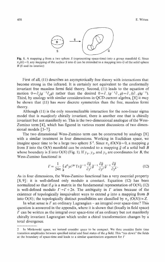
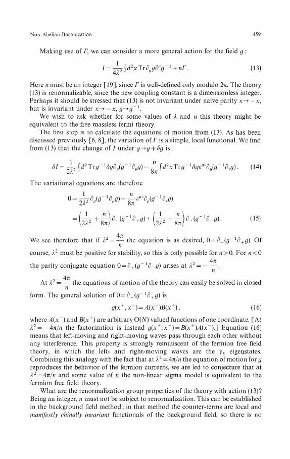
Fig. 1. A mapping g from a two sphere S (representing space-time) into a group manifold G. Sinceπ2(G) = 0, any mapping of the surface S into G can be extended to a mapping into G of the solid sphereB (S and its interior)

First of all, (11) describes an asymptotically free theory with interactions thatbecome strong in the infrared. It is certainly not equivalent to the conformallyinvariant free massless fermi field theory. Second, (11) leads to the equation ofmotion O = dμ(g~1dμg) rather than the desired O = d_{g~1d+g) = δ + ((δ_g)g~1).Third, by analogy with similar considerations in QCD current algebra, [8] it maybe shown that (11) has more discrete symmetries than the free, massless fermitheory.

Although (11) is the only renormalizable interaction for the non-linear sigmamodel that is manifestly chirally invariant, there is another one that is chirallyinvariant but not manifestly so. This is the two-dimensional analogue of the Wess-Zumino term [4], which has figured in various recent discussions of two dimen-sional models [5-7].

The two dimensional Wess-Zumino term can be constructed by analogy [8]with a similar treatment in four dimensions. Working in Euclidean space, weimagine space time to be a large two sphere S2. Since π 2 (O(iV)) = 0, a mapping gfrom S into the O(N) manifold can be extended to a mapping g of a solid ball Bwhose boundary is S into O(iV) (Fig. 1). lfyv y2, and y3 are coordinates for B, theWess-Zumino functional is

As in four dimensions, the Wess-Zumino functional has a very essential property[8,9]: it is well-defined only modulo a constant. Equation (12) has beennormalized so that if g is a matrix in the fundamental representation of O(iV), (12)is well-defined modulo Γ->Γ + 2π. The ambiguity in Γ arises because of theexistence of topologically inequivalent ways to extend g into a mapping from Binto O(JV); the topologically distinct possibilities are classified by π 3 (O(iV)) —Z.

In what sense is Γ an ordinary Lagrangian - an integral over space-time? Thisquestion is answered in the appendix, where it is shown that (locally in field space)Γ can be written as the integral over space-time of an ordinary but not manifestlychirally invariant Lagrangian which under a chiral transformation changes by atotal divergence.

2 In Minkowski space, we instead consider space to be compact. We then consider finite timetransition amplitudes between specified initial and final states of the g field. This "ties down" the fieldsat the boundary of space-time and leads to a similar quantization argument for Γ

Non-Abelian Bosonization 459

Making use of Γ, we can consider a more general action for the field g:

/ = ^ I ί d 2 x T r 3 μ f l f 3 ^ - 1 + n Γ . (13)

Here n must be an integer [19], since Γ is well-defined only modulo 2π. The theory(13) is renormalizable, since the new coupling constant is a dimensionless integer.Perhaps it should be stressed that (13) is not invariant under naive parity χ-> — x,but is invariant under x—• — x, g-^g'1.

We wish to ask whether for some values of λ and n this theory might beequivalent to the free massless fermi theory.

The first step is to calculate the equations of motion from (13). As has beendiscussed previously [6, 8], the variation of Γ is a simple, local functional. We findfrom (13) that the change of / under g-*g + δg is

The variational equations are therefore

4πWe see therefore that if λ2 — — the equation is as desired, 0 = d_(g 1d + g). Of

course, λ2 must be positive for stability, so this is only possible for n>0. For n<04π

the parity conjugate equation 0 = d + (g~1d_g) arises at λ2 = .

4πAt λ2 = — the equations of motion of the theory can easily be solved in closed

nform. The general solution of 0 = d_(g~1d + g) is

g(x\χ-) = A(χ-)B(x + ) , (16)

where A(x~) and B(x+) are arbitrary O(N) valued functions of one coordinate. [Atλ2 = — 4π/n the factorization is instead g(x + ,x~) = B(x + )A(x~).^ Equation (16)means that left-moving and right-moving waves pass through each other withoutany interference. This property is strongly reminiscent of the fermion free fieldtheory, in which the left- and right-moving waves are the y5 eigenstates.Combining this analogy with the fact that at λ2 = 4π/n the equation of motion for greproduces the behavior of the fermion currents, we are led to conjecture that atλ2=4π/n and some value of n the non-linear sigma model is equivalent to thefermion free field theory.

What are the renormahzation group properties of the theory with action (13)?Being an integer, n must not be subject to renormahzation. This can be establishedin the background field method in that method the counter-terms are local andmanifestly chinally invariant functionals of the background field, so there is no

460 E. Witten

4

3

2

I

l/λ 2

-I

- 2

- 3

-4\

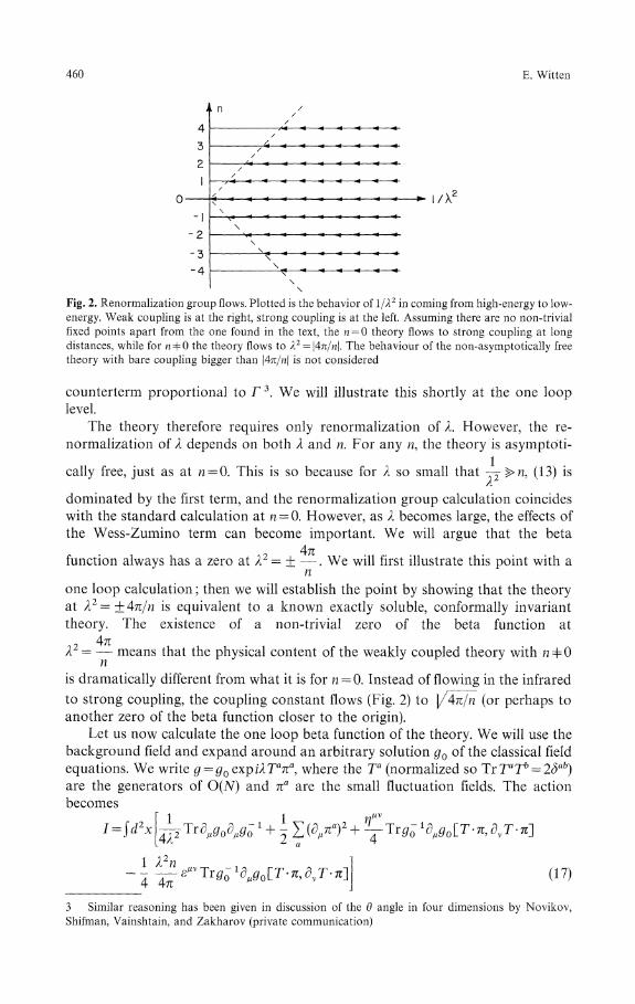
\Fig. 2. Renormalization group flows. Plotted is the behavior of l/λ2 in coming from high-energy to low-energy. Weak coupling is at the right, strong coupling is at the left. Assuming there are no non-trivialfixed points apart from the one found in the text, the n = 0 theory flows to strong coupling at longdistances, while for rcφO the theory flows to λ2 = \4π/n\. The behaviour of the non-asymptotically freetheory with bare coupling bigger than \4π/n\ is not considered

counter term proportional to Γ 3 . We will illustrate this shortly at the one looplevel.

The theory therefore requires only renormalization of λ. However, the re-

normalization of λ depends on both λ and n. For any n, the theory is asymptoti-

cally free, just as at n = 0. This is so because for λ so small that -j >n, (13) is

dominated by the first term, and the renormalization group calculation coincideswith the standard calculation at n = 0. However, as λ becomes large, the effects ofthe Wess-Zumino term can become important. We will argue that the beta

4πfunction always has a zero at λ2 = ± — . We will first illustrate this point with a

none loop calculation then we will establish the point by showing that the theoryat λ2=±4π/n is equivalent to a known exactly soluble, conformally invarianttheory. The existence of a non-trivial zero of the beta function at

4πλ2= — means that the physical content of the weakly coupled theory with nφO

is dramatically different from what it is for n = 0. Instead of flowing in the infrared

to strong coupling, the coupling constant flows (Fig. 2) to ]/4π/n (or perhaps to

another zero of the beta function closer to the origin).Let us now calculate the one loop beta function of the theory. We will use the

background field and expand around an arbitrary solution g0 of the classical fieldequations. We write g = g0 expUTV, where the Ta (normalized so Tr TaTb = 2δab)are the generators of O(N) and πa are the small fluctuation fields. The actionbecomes

1 = \d x

1 λ2^

4 4π(17)

3 Similar reasoning has been given in discussion of the 0 angle in four dimensions by Novikov,Shifman, Vainshtain, and Zakharov (private communication)

Non-Abelian Bosonization 461

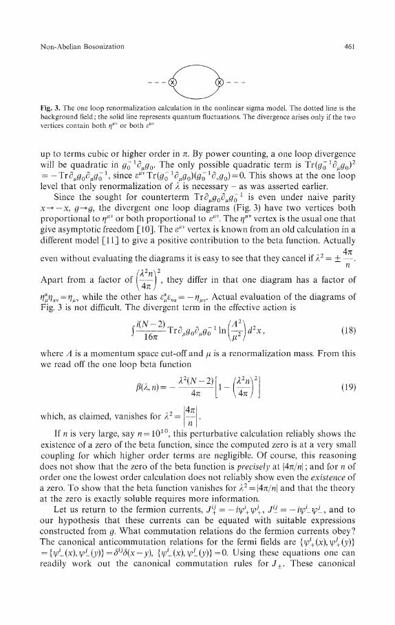
Fig. 3. The one loop renormalization calculation in the nonlinear sigma model. The dotted line is thebackground field the solid line represents quantum fluctuations. The divergence arises only if the twovertices contain both ημv or both εμv

up to terms cubic or higher order in π. By power counting, a one loop divergencewill be quadratic in gQXdμgQ. The only possible quadratic term is Tr(^ 0 " 1 ^ μ ^ 0 ) 2

- -TrdμgQdμg~\ since sμvΎΐ{g~ίdμgo){g~1dvgo) = 0. This shows at the one looplevel that only renormalization of λ is necessary - as was asserted earlier.

Since the sought for counterterm ΎrdμgodμgQ x is even under naive parityx-+—x, g-^g, the divergent one loop diagrams (Fig. 3) have two vertices bothproportional to ημv or both proportional to εμv. The ημv vertex is the usual one thatgive asymptotic freedom [10]. The εμv vertex is known from an old calculation in adifferent model [11] to give a positive contribution to the beta function. Actually

4πeven without evaluating the diagrams it is easy to see that they cancel if λ2 = ± —-.

( T 2 \ 2

, they differ in that one diagram has a factor ofAn)

ηa

μηav = η v while the other has εa

μεva = — ημv. Actual evaluation of the diagrams ofFig. 3 is not difficult. The divergent term in the effective action is

ΛN-2) (Λ2\(Λ\

ΐ&Γ μθo μQo \jJ) ' ( }

where A is a momentum space cut-off and μ is a renormalization mass. From thiswe read off the one loop beta function

4πwhich, as claimed, vanishes for λ2 = —

nIf n is very large, say n = 1010, this perturbative calculation reliably shows the

existence of a zero of the beta function, since the computed zero is at a very smallcoupling for which higher order terms are negligible. Of course, this reasoningdoes not show that the zero of the beta function is precisely at \4π/n\ and for n oforder one the lowest order calculation does not reliably show even the existence ofa zero. To show that the beta function vanishes for λ2 = |4π/n| and that the theoryat the zero is exactly soluble requires more information.

Let us return to the fermion currents, Jι{ = — π//+φJ

+, JijL = —ίψLψL, and toour hypothesis that these currents can be equated with suitable expressionsconstructed from g. What commutation relations do the fermion currents obey?The canonical anticommutation relations for the fermi fields are {ψί

+(x),ψj

+(y)}= {ψι_(x\ψL(y)} =διjδ(x — y\ {ψι_(x),ψL(y)} =0. Using these equations one canreadily work out the canonical commutation rules for J±. These canonical

462 E. Witten

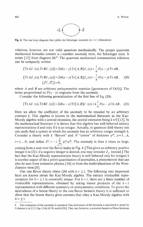
OFig. 4. The one loop diagram that yields the Schwinger anomaly in 1 + 1 dimensions

relations, however, are not valid quantum mechanically. The proper quantummechanical formulas contain a c-number anomaly term, the Schwinger term. Itarises [12] from diagram (4)4. The quantum mechanical commutation relationscan be compactly written

[ΎrAJ _(x\ΎrBJ _(y)~] = 2iδ(x- y)TrlA, B~]J _(x)+ -δf(x- y)TrAB,n

[ττAJ+(x\ΎτBJ + (y)-]=2iδ(x-y)ΎτlA,Bp+(x)- l-δ\x-y)ΊrAB, (20)

I W + ] = O,

where A and B are arbitrary antisymmetric matrices [generators of O(iV)]. Theterms proportional to δ'(x — y) originate from the anomaly.

Consider the following generalization of the first line of Eq. (20):

[ΎrAJ Jx),TrBJ _{yft=2iδ(x- y)Ύr[A,B]J _{x) + k-δ'{x- y)ΎrAB. (21)π

Here we allow the coefficient of the anomaly to be rescaled by an arbitraryconstant k. This algebra is known in the mathematical literature as the Kac-Moody algebra with a central extension, the central extension being fc + O [13]. Inthe mathematical literature it is shown that this algebra has well-behaved unitaryrepresentations if and only if k is an integer. Actually, in quantum field theory onecan easily find a system in which the anomaly has an arbitrary integer strength k.Consider a theory with k "flavors" and N "colors" of fermions ψia, a = l...k,

k

i=l...N, and define Jιί = —i Σ ψ™ψjL The anomaly is then k times as large,a— 1

coming from a sum over the flavor index in Fig. 4. [This gives an arbitrary positiveinteger k in (21) if a negative integer is desired, one may consider J + instead.] Thefact that the Kac-Moody representation theory is well behaved only for integral kis another aspect of the a priori quantization of anomalies, a phenomenon that canalso be seen from instant on physics [14] or from the multivaluedness of the Wess-Zumino term [8].

Our one flavor theory obeys (20) with k= ±1. The following very importantfacts are known about the Kac-Moody algebra. The unitary irreducible repre-sentation for k= ± 1 is essentially unique. For k> 1, there are a finite number ofirreducible representations, obtained by taking tensor products of the fc = lrepresentation with different symmetry or antisymmetry conditions. To prove theequivalence of a boson theory to the one flavor fermion theory it is sufficient toshow that the boson theory gives currents that obey a Kac-Moody algebra with

4 The evaluation of the anomaly is standard. One derivation of this formula is described in detail byColeman et al. [12, Eqs. (3.4), (4.19), and (4.28)]. They use, however, a notation based on Dirac fermions

Non-Abelian Bosonization 463

\\

\\

\ / I\

\\

\ τ = 0\

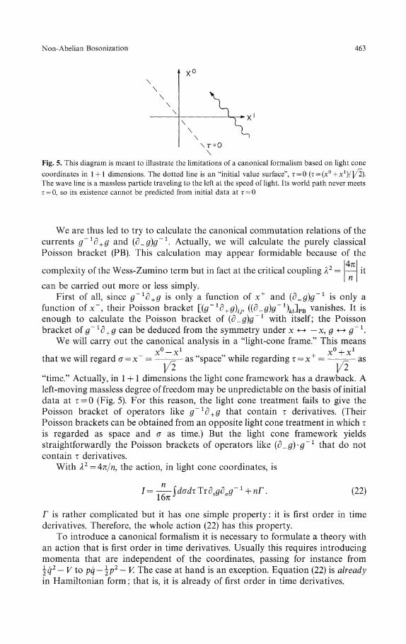
Fig. 5. This diagram is meant to illustrate the limitations of a canonical formalism based on light cone

coordinates in 1 + 1 dimensions. The dotted line is an "initial value surface", τ = 0 (τ = (x° +x1)/y2).

The wave line is a massless particle traveling to the left at the speed of light. Its world path never meets

τ = 0, so its existence cannot be predicted from initial data at τ = 0

We are thus led to try to calculate the canonical commutation relations of thecurrents g~xd+g and (d_g)g~1. Actually, we will calculate the purely classicalPoisson bracket (PB). This calculation may appear formidable because of the

4πcomplexity of the Wess-Zumino term but in fact at the critical coupling λ2 =

can be carried out more or less simply.First of all, since g~xd+g is only a function of x+ and {d_g)g~1 is only a

function of x~, their Poisson bracket [_{g~ιd + g)ip {{^_g)g~ι)kl\Έ vanishes. It isenough to calculate the Poisson bracket of (d_g)g~1 with itself; the Poissonbracket oϊ g~1d + g can be deduced from the symmetry under x <-• — x,g<r^g~1.

We will carry out the canonical analysis in a "light-cone frame." This meansx°-x1 x° + x1

that we will regard σ = x" = -=- as "space" while regarding τ = x+ = =— as1/2 1/2

"time." Actually, in 1 + 1 dimensions the light cone framework has a drawback. Aleft-moving massless degree of freedom may be unpredictable on the basis of initialdata at τ = 0 (Fig. 5). For this reason, the light cone treatment fails to give thePoisson bracket of operators like g~1d + g that contain τ derivatives. (TheirPoisson brackets can be obtained from an opposite light cone treatment in which τis regarded as space and σ as time.) But the light cone framework yieldsstraightforwardly the Poisson brackets of operators like (d_g)-g~1 that do notcontain τ derivatives.

With λ2 = 4π/n, the action, in light cone coordinates, is

Γ is rather complicated but it has one simple property: it is first order in timederivatives. Therefore, the whole action (22) has this property.

To introduce a canonical formalism it is necessary to formulate a theory withan action that is first order in time derivatives. Usually this requires introducingmomenta that are independent of the coordinates, passing for instance from^q2 — V to pq — \p2 — V. The case at hand is an exception. Equation (22) is alreadyin Hamiltonian form that is, it is already of first order in time derivatives.

464 E. Witten

In one other way, (22) differs from usual experience. In the light cone non-linear sigma model it is not convenient to split the dynamical variables intocoordinates and momenta. Let us discuss, therefore, how Poisson brackets may ingeneral be computed without making an explicit choice of p's and q's.

Consider a theory with dynamical variables φι and an arbitrary action that isfirst order in time derivatives:

I=SdtAt{φ)^. (23)

(The action may also contain terms independent of time derivatives such termsare ignored in computing Poisson brackets.) We calculate the change in / under anarbitrary infinitessimal variation φι-^φι + δφι:

J \dφJ at at

Define a matrix Fίj = diAj — djAi as the coefficient of δφ1——. Notice that Ftj is

always antisymmetric. Let Fjk be the universe matrix of Ftj (so FjkFki = δj).5 Thenthe Poisson bracket of any two functions on phase space X and Y is defined by

ff. (25)In the simple case in which the φι are decomposed into coordinates and momentaqι and p\ and in which the part of the action containing time derivatives is

.άd^dt^p1——, (25) agrees with the usual definition of Poisson brackets.

In this calculation it is unnecessary to choose an explicit set of coordinates φι

for the classical phase space. (Such a choice would be very awkward in the non-linear sigma model becuase of the nonlinearity of the phase space.) It is enoughto have a basis of tangent vectors to the phase space (analogous to the tetrad ingeneral relativity). The matrices Ftj and Fjk may be constructed relative to anysuch basis. In the non-linear sigma model a very convenient basis of tangents tothe phase space are the matrices g~ 1δg(σ). The matrix F must act both on the Liealgebra index of g~1δg(σ) and on σ.

In this basis, it is very easy to calculate the matrix F in the non-linear sigmamodel. From (14), with λ2 = 4π/n, the variation of the action is

lδvΛ- (26)

5 If this inverse does not exist, one must introduce "constraints.") This does not occur in the case at

hand

Non-Abelian Bosonization 465

From (26) we see that F is 1® , where " 1 " acts on the Lie algebra index andn d 4π dσ

- — acts on the spatial coordinate. The inverse matrix is, of course4π dσ

n \We now wish to apply definition (25) of the Poisson bracket with

X = ΊτA — g~\σ\ Y = ΊΐB~^g~1(σ'). Note that (25) can be understood asdσ dσ

follows. First calculate δXδY= —r ——. δφίδφj then replace δφιδφj by Fij. So wecφ dφJ

calculate δX:

)^(gδg(σ)). (27)dσ

δY is evaluated similarly, so

^ ι ^ 1 δ g ( σ f ) ) . (28)^(gδg(σ))Ίτg(σ)Bg(σ)^7(gδg(σdσ dσ

After evaluating δXδY= —Γ -—Γδφiδφ\ the next step is to replace δφιδφj

oφι oφJ

with Fιj. In our problem the role of δφι and δφj is played by (g~1δg(σ))a and(g~ίδg(σ'))b (here we explicitly exhibit - temporarily - the Lie algebra indices aand b carried by these matrices). In view of our previous determination of Ftj

4πand Fι\ we are to replace (g~1δg(σ))a(g~ίδg(σ))b by δab — θ(σ,σ') where 0(σ,σ') is

an inverse of -—. Hence —{g~ιδg(σ))a'—-(g~1δg(σ'))b is replaced by δab

dσ dσ dσ n dσ

•-—θ{σ-σ')=-δab — δ\σ-σ'\ For the Poisson bracket of X and Y we getdσ n

therefore

4π[X, Y]PB= - —δ\σ-σ')Ύvg-\σ)Ag{σ)g-\σ>)Bg(σ')

= -—δ(σ-σ/)Ύr[A,B~] — g-1-—δ'(σ-σ')TrAB. (29)n dσ n

Bearing in mind the definition of X and Y and the relation between Poissonbrackets and quantum mechanical commutation relations, this corresponds to the

466 E. Witten

commutation relations

dσJ y " d σ ° v

4π da _ λ 4π= — i δ ( σ — σ)Tr\_A,n] — g Λ id (σ — σ)ΎrAB. (30)

n dσ n

Now, let us compare this to the Kac-Moody algebra (21). We see that they

coincide if k = n and if J_ is identified with r-g"1-2π dσ

Now, that conclusions can we draw? In the nonlinear sigma model and inEq. (30), n is an integer because of the multivaluedness of the Wess-Zuminocoupling. In (21) k is an integer because only then does the Kac-Moody algebrahave well-behaved unitary representations. We see that single valuedness of eι\required in quantum mechanics for mathematical consistency, leads to a Kac-Moody algebra with properly normalized central charge.

Second, the theory at λ2 = 4π/n really does have a vanishing β function, becauseit is known [15] that the irreducible representation of the Kac-Moody algebra isconformally invariant (can be extended to the semi-direct product of the Kac-Moody algebra with the conformal algebra).

Third, and most important, it follows from Eq. (30) that the non-linear sigmamodel with n=l and λ2 = 4π is equivalent to the free field theory of N masslessMajorana fermions. For, with the identifications

(31)

dτj '

the currents of these theories obey the same algebra [Eqs. (20) and (30)], and, ashas been mentioned, this algebra has an essentially unique irreducible representa-tion. (The Hubert spaces of the quantum theories in question furnish irreduciblerepresentations of the current algebras because no operators commute with allthe currents. This has been proved [13] in the fermi case and also [16] in thebose case.6) The Kac-Moody representation is not quite unique, but the non-uniqueness just refers to superselection rules and boundary conditions in thequantum field theory.

Moreover, the Hamiltonian H and the momentum operator P of the free fermitheory coincide with those of the non-linear sigma model at the special values of

6 Our discussion of the non-linear sigma model is closely related to the discussion of the Kac-Moodyrepresentations in [16]. The phase space of our theory in the light cone frame is a complex manifold,the loop space Z of O(N). (Actually, this is only half the phase space of the theory, since it omits left-moving waves. The full phase space is Z x Z.) The operator Ftj that we have constructed represents thefirst Chern class of a holomorphic line bundle E over Z. The Hubert space of the theory is the space ofholomorphic sections of E. This construction generalizes some classical theorems about repre-sentations of finite dimensional Lie groups to the Kac-Moody system. The novelty of our discussion ofthe non-linear sigma model is to show that the construction of Kac-Moody representations justmentioned can be realized by canonical quantization of a quantum field theory

Non-Abelian Bosonization 467

the couplings under discussion. This can be seen in various ways. Because theHubert spaces form irreducible representations of the current algebras, H and Pare uniquely determined in each case by their commutation relations with thecurrents. These commutation relations are suitable H and P generate translationsin both the bose and fermi theories. A more explicit argument is the following. Inthe fermi theory one can show H +P = constlim jdxJιl(x + ε)Jil(x), and a similar

formula for H — P in terms of J_. (This is not a canonical equation. One muststudy the short distance behavior of the product of currents, and subtract aninfinite c-number.) On the other hand, in the bose theory one can calculatecanonically an equivalent formula

r ( -Λ dg

= const \dxTv\g -—\ dτ

(and similarly for H — P). In view of (31) these relations show that H and P of thebose theory equal those of the fermi theory.

By introducing several fermion flavors, it is possible to make a bose-fermitranslation also for w+1. Consider a theory with N "colors" and n "flavors" ofMajorana fermions ψia, j=l...JV and a=l...n. We can define currents

These currents generate O(N)L

x O(N)R x O(n)L x O(n)R. The O(N)L x O{N)R current commutators have anom-alies of strength n. The O(n)L x O(ή)R current commutators have anomalies ofstrength N. The free field theory Hubert space is an irreducible representation[17] of the combined current algebra.

An equivalent bose theory is a theory with two fields g and h g takes values inO(N) and h in O(ή). For g we take a Wess-Zumino coupling n and λ2 = 4π/n for hwe take a Wess-Zumino coupling N and λ2 = 4π/N. g and h are decoupled,corresponding to the fact that at the fermion level amplitudes with a product ofO(N)LxO(N)RxO(n)LxO(n)R currents factorize [18] as a product ofO(N)L x O(N)R amplitudes and O(ή)L x O(ή)R amplitudes. The Hamiltonian andmomentum operators of xpίa can be identified with the sum of those constructedfrom g and h.

As we have discussed, Eq. (31) generalizes to the non-abelian case the equation

ψyμψ= ——zβ dvφ of conventional bosonization. In conventional bosonization,

1/πthere also are formulas ψxp = Mcos j/4πφ, ψiγ5ψ = M sin ]/4πφ (Mis a re-normalization mass). What are the analogues of those formulas here?

Let Q^= — iψί_ψ + k. We would like to translate Q[ into the bose language. Thecommutators of Qlk with the fermion currents are as follows:

Uΰ M> efGO] = - iδ(x - y)(δJkQί(y) - <5ifcβ/(j,)],

Uΐj (x), βfϋO] = - iδ{χ - yWjjQmy) - δiXφ)).

We must therefore find in the bose theory operators obeying the algebra (32). Oneneed not look far. The matrix elements gι.(x) of the matrix g are the required

468 E. Witten

operators. Canonically,

1 ίdg _ \ij ]7Γ~\~r- Q 1(x)\ ><fi(y)\ — — iδ(x — y)(δjkqli(v) — διkqJ,(y)),2π\dσy y ') ί ! w ; | v y n UιKyj w "

(33)

= -iδ(x-y)(&ιgk

i{y)-δilφ)).

I The evaluation of (33) is simple for the following reason. From (30) we know that

ίdx—-g~~ι and \dxg~x -— generate chiral O(JV) x O(N). Therefore, (33) holds up todσ dτ

total derivatives that vanish after integrating over x. By virtue of locality anddimensional analysis - g is dimensionless - there are no such possible terms. For

the same reason, there can be no anomaly in (33) quantum mechanically.

At least heuristically, it appears that Qk(x) and gk(x) are uniquely characterized(up to normalization) by the relations (32) and (33). For instance, in the free fermitheory one cannot find another operator that transforms like Qk{x\ so we are ledto conclude

c), (34)

where (as in the conventional bosonization) M is a mass that depends on therenormalization procedure for the bosonic operator. It should be noted that -while — zτ/;i_φJ

+ has canonical dimension one - gι. is dimensionless classically. SoEq. (34) is possible only if gι has anomalous dimension one in the fixed pointtheory with n = 1.

Equation (34) is a generalization of the conventional bosonization formulas, inwhich ψψ and ψίy5ψ are identified with matrix elements of the O(2) matrix

/ cos |/4πφ sin]/4πφ\ . ΛΛv v . Of course, in the free bose field theory, it is easy to see

\ — sin ]/4πφ cos ]/4π φ/that cos ]/ΐπφ and sin ]/4πφ do have anomalous dimension one.

Equation (34) can be tested in the following way. We have identified iψ[ψj

with ±-(^g-Al =±-Σ^Γgi(g-if Since g is orthogonal, {g-'f^gl So2π \dx J 2π k dx J J

j k

j = ^-Σ~j-^gi If we identify gι

} with —~-xpι_ψj+, we are led to require£JL fa CLJv -1V.L

) (35)

At first sight Eq. (35) looks preposterous. It relates an operator quadratic inspinors to one quartic in spinors. However, to understand the right-hand side of(35), we must study the small A behavior of

1 r\

Ύ2 ί d2yj^T(ΨrΨk

+(y)ψ7Ψk

+(x)). (36)Δ iyo-xo <A/2 oy

\y1-χί <A/2

Non-Abelian Bosonization 469

N d NSince £ -—^T{ψ£(y)ψ£{x)) = Nδ2(x-yl (36) has a piece - ~jψ. ψ. (x). This is

k=i oy Δ

the most singular part of (36), as A ->0. Equation (35) must be understood to meanthat the operator on the left-hand side equals the most singular part of theoperator on the right-hand side. Note that while A is cut-off dependent, the massM appearing in — iψ^ψΐ(x) = Mgi

j(x) is also cutoff dependent [since — iψ^ψ~l hasno anomalous dimension, but as already noted gι must have anomalous dimensionone in the equivalent bose theory, if the relation — iψ^ψJ~(x) = Mglj(x) holds].Evidently, in view of (35) and (36), the product MA is cut-off independent.Equation (35) holds in the limit as M->oo and Δ-+Q with MA fixed. While thesemanipulations are somewhat bizarre, the same bizarre manipulations are neededin conventional bosonization to show the consistency of the relations

μ μvdφ, ψψ = M cos ]/4πφ, ψίγ5ψ = Msm ]/4πφ.ψyψ= εdvφ,

1/πThis completes the dictionary of bosonization of fermi bilinears. Given the

dictionary, it should be clear that the bosonization can be carried out also forarbitrary massive or interacting fermi theories. For instance, a fermion bare mass

N

mψψ = mi ]Γ ψk_ψ\ can be included by adding to the Lagrangian a termk= 1

N

proportional to Σ g\ = Trg. A {xpxp)2 coupling becomes (Tr#)2. One can likewisei = 1

study gauge theories in this way. For instance, in the fermion language one maychoose to gauge an arbitrary anomaly free subgroup H of chiral O(Λ0 x O(N). Thecorresponding theory can be studied in the bose language by gauging the samesubgroup H of the symmetry group of the nonlinear sigma model. One will belimited to anomaly free groups H - as one should be - because only for anomalyfree groups does the Wess-Zumino term have a gauge invariant generalization [8].

Various applications of the present work can be imagined, but will not beexplored here. The non-abelian bosonization may help in understanding 1 + 1dimensional field theories. It may be helpful in understanding the Callan-Rubakoveffect, which is described by an effective 1 + 1 dimensional s-wave field theory. Andthe conformally invariant theory with λ2 = 4π/n may provide a starting point forconstructing generalizations of the usual string theories.

Appendix: Explicit Form of the Wess-Zumino Functional

In this appendix we will work out an explicit formula for the Wess-Zuminofunctional in the simplest case of an SU(2) non-linear sigma model in two space-time dimensions. We will use an index free notation, so antisymmetric tensors ωijk

are denoted simply as ω, and the curl of ω, (d^jkl ± cyclic permutations) is denoteddω. Differentials are considered to anticommute, so dxdy = — dydx and (dx)2 = 0, ifx and y are functions.

First let us write the Wess-Zumino functional in an abstract form. On thegroup manifold of any simple, non-abelian group G, there is a G x G invariant third

470 E. Witten

rank tensor field ω. ω obeys dω = 0, and locally but not globally ω = dλ for somesecond rank tensor field λ. ω may be normalized so that its integral over any threesphere in G is an integral multiple of 2π.

Let B be a three-dimensional ball whose boundary, the two sphere S, isidentified with space time. Given a mapping g from S into G, which has beenextended to a mapping (also denoted g) from B into G, the Wess-Zuminofunctional is defined as

Γ=$g*-ω=$g*-dλ = \g*-λ=\g*-λ. (37)B B δB S

Here g* is the "pull-back" of differential forms. In the third step of (37) dB = S isthe boundary of B; Stokes' theorem has been used. The last formula in (37)exhibits Γ as the integral of an ordinary two-dimensional Lagrangian. In concreteterms, the meaning of this formula as follows. Let φι be a set of coordinates for thegroup manifold G. Let λtj be the components of the anti-symmetric tensor λ. Thenthe mapping g :S-^G can be described by means of functions φ\ and

Γ = J d'xε^λ^φ^d^d^'. (38)

Equation (38) has "Dirac string" type singularities, because the defining equationof λ, ω = dλ, can be solved only locally on the group manifold.

Equation (38) is G x G invariant, although not manifestly so. Under a G x Gdβ. δβ. .

transformation λ transforms as λij-+λiJ+ ^~r — —± for some β:{φ). Sodφ oφJ

δΓ = J d2xε^{diβj - djβ^φ'd^ = 2$d2x~ (s»vβjdvφj), (39)

and Γ changes by a total divergence whose integral vanishes.Now let us construct explicit formulas for the simplest non-abelian group

SU(2). The SU(2) manifold is a three sphere it can be described by polar angles ψ,0, φ with line element ds2 = dψ2 + sin2ψ(dθ2 + sin2 θdφ2). The only SU(2)x SU(2)invariant third rank antisymmetric tensor is the Levi-Civita tensor or volumeform, so

ω = — sin2 ψ sin θ dψdθdφ. (40)π

Note the normalization of (40). Since the volume of the SU(2) manifold is 2π2, (40)is chosen so that the integral of ω over the whole manifold is 2π.

The equation ω = dλ can be solved in many ways, for instance

X= —φsin2xpsinθdψdθ. (41)π

[Recall (dψ)2 = (dθ)2 = 0.] So given a mapping of space-time into SU(2), theproperly normalized Wess-Zumino interaction is

Γ = -\d2xφ{x) ύn2xp{x) sinθ(x)εμvdμψ(x)dvθ(x). (42)

Non-Abelian Bosonization 471

[In this parametrization, the Dirac-string type singularities occur at θ(x) = 0 or π.For at θ = 0 or π, everything should be independent of φ. This is not true in Eq.(42). In the case of the group SU(2), it is possible to choose another para-metrization that is singular only at a single point on the group manifold.]

Formulas similar to (42) can be constructed for other groups and also for theWess-Zumino interaction in four dimensions. These formulas are not veryenlightening, however.

Acknowledgements. I wish to thank A. Feingold and I. Frenkel for discussions about Kac-Moodyalgebras, and D. J. Gross for suggesting a test of Eq. (34). I also wish to acknowledge discussions ofbosonization and related matters with S. Coleman and D. Olive.

References

1. Coleman, S.: Quantum sine-Gordon equation as the massive Thirring model. Phys. Rev. D l l ,2088 (1975)

2. Mandelstam, S.: Soliton operators for the quantized sine-Gordon equation. Phys. Rev. D l l , 3026(1975)

3. Baluni, V.: The Bose form of two-dimensional quantum chromodynamics. Phys. Lett. 90 B, 407(1980)

Steinhardt, P.J.: Baryons and baryonium in QCD 2 . Nucl. Phys. B 176, 100 (1980)

Amati, D., Rabinovici, E.: On chiral realizations of confining theories. Phys. Lett. 101B, 407 (1981)4. Wess, J., Zumino, B.: Consequences of anomalous word identities. Phys. Lett. 37 B, 95 (1971)5. D'Adda, A., Davis, A.C., DiVecchia, P.: Effective actions in non-abelian theories. Phys. Lett. 121B,

335 (1983)6. Polyakov, A.M., Wiegmann, P.B.: Landau Institute preprint (1983)7. Alvarez, O.: Berkeley preprint (1983)8. Witten, E.: Global aspects of current algebra. Nucl. Phys. B (to appear)9. Novikov, S.P.: Landau Institute preprint (1982)

10. Polyakov, A.M.: Interaction of Goldstone particles in two dimensions. Applications to fer-romagnets and massive Yang-Mills fields. Phys. Lett. 59 B, 79 (1975)Belavin, A.A., Polyakov, A.M.: Metastable states of two-dimensional isotropic ferromagnets.JETP Lett. 22, 245 (1975)

11. Nappi, C.R.: Some properties of an analog of the chiral model. Phys. Rev. D21, 418 (1980)12. Goto, T., Imamura, I.: Note on the non-perturbation-approach to quantum field theory. Prog.

Theor. Phys. 14, 396 (1955)Schwinger, J.: Field-theory commutators. Phys. Rev. Lett. 3, 296 (1959)Jackiw, R.: In: Lectures on current algebra and its applications, Treiman S.B., et al. (eds.): Princeton,NJ: Princeton University Press 1972Coleman, S., Gross, D., Jackiw, R.: Fermion avatars of the Sugawara model. Phys. Rev. 180,1359(1969)

13. Kac, V.G.: J. Funct. Anal. Appl. 8, 68 (1974)Lepowsky, J., Wilson, R.L.: Construction of the affine Lie algebra. Λ^l). Commun. Math. Phys.62, 43 (1978)Frenkel, I.B.: Spinor representations of affine Lie algebras. Proc. Natl. Acad. Sci. USA 77, 6303(1980); J. Funct. Anal. 44, 259 (1981)Feingold, A.J., Frenkel, I.B.: IAS preprint (1983)

14. Belavin, A.M., Polyakov, A.M., Schwar, A.S., Tyμpkin, Yu.S.: Pseudoparticle solutions of theYang-Mills equations. Phys. Lett. 59 B, 85 (1975)'t Hooft, G.: Symmetry breaking through Bell-Jackiw anomalies. Phys. Rev. Lett. 37, 8 (1976);Computation of the quantum effects due to a four-dimensional pseudoparticle. Phys. Rev. D14,3432 (1976)Callan, C.G., Jr., Dashen, R., Gross, D J . : The structure of the gauge theory vacuum. Phys. Lett.63 B, 334(1976)Jackiw, R., Rebbi, C.: Vacuum periodicity in a Yang-Mills quantum theory. Phys. Rev. Lett. 37,172 (1976)

472 E. Witten

15. Segal, G.: Unitary representations of some infinite-dimensional groups. Commun. Math. Phys. 80,301 (1981)Frenkel, I., Kac, V.G.: Basic representations. Invent Math. 62, 23 (1980)

16. Kac, V.G., Peterson, D.H.: Spin and wedge representations of infinite-dimensional Lie algebrasand groups. Proc. Natl. Acad. Sci. USA 78, 3308 (1981)

17. Frenkel, I.: Private communication18. Frishman, Y.: Quark trapping in a model field theory. Mexico City 1973. Berlin, Heidelberg, New

York: Springer 197519. Deser, S., Jackiw, R., Templeton, S.: Three-dimensional massive gauge theories. Phys. Rev. Lett.

48, 975 (1982); Topologically massive gauge theories. Ann. Phys. (NY) 140, 372 (1982)

Communicated by A. Jaffe

Received September 29, 1983