NIOSH Method No. 3900 backup data report · Method 3900. The focus of the canister method...
67
NIOSH Manual of Analytical Methods (NMAM) 5th Edition BACKUP DATA REPORT NIOSH Method No. 3900 Title: Volatile Organic Compounds, C1 to C10, Canister Method Analyte: ethanol, 2-propanol, acetone, 2,3-butanedione, 2,3-pentanedione, 2,3-hexanedione, dichloromethane, trichloromethane, hexane, benzene, toluene, ethylbenzene, o-xylene, m- xylene, p-xylene, methyl methacrylate, α-pinene, and d-limonene Author/developer: Ryan LeBouf, NIOSH Date: 8/30/2018 Disclaimer: Mention of any company or product does not constitute endorsement by the National Institute for Occupational Safety and Health, Centers for Disease Control and Prevention. In addition, citations to websites external to NIOSH do not constitute NIOSH endorsement of the sponsoring organizations or their programs or products. Furthermore, NIOSH is not responsible for the content of these websites. All web addresses referenced in this document were accessible as of the publication date.
Transcript of NIOSH Method No. 3900 backup data report · Method 3900. The focus of the canister method...
NIOSH Manual of Analytical Methods (NMAM) 5th Edition
BACKUP DATA REPORT
NIOSH Method No. 3900
Title: Volatile Organic Compounds, C1 to C10, Canister Method
Analyte: ethanol, 2-propanol, acetone, 2,3-butanedione, 2,3-pentanedione, 2,3-hexanedione, dichloromethane, trichloromethane, hexane, benzene, toluene, ethylbenzene, o-xylene, m- xylene, p-xylene, methyl methacrylate, α-pinene, and d-limonene
Author/developer: Ryan LeBouf, NIOSH
Date: 8/30/2018
Disclaimer: Mention of any company or product does not constitute endorsement by the National Institute for Occupational Safety and Health, Centers for Disease Control and Prevention. In addition, citations to websites external to NIOSH do not constitute NIOSH endorsement of the sponsoring organizations or their programs or products. Furthermore, NIOSH is not responsible for the content of these websites. All web addresses referenced in this document were accessible as of the publication date.
BACKUP DATA REPORT NMAM Method No 3900 Volatile Organic Compounds, C1 to C10, Canister Method Substance C1-C10 volatile organic compounds
Chemicals Used for Evaluation Specific chemicals tested were ethanol, 2-propanol, acetone, 2,3-butanedione, 2,3-pentanedione, 2,3- hexanedione, dichloromethane, trichloromethane, hexane, benzene, toluene, ethylbenzene, o-xylene, m,p- xylene, methyl methacrylate, ɑ-pinene, d-limonene. Custom gas standards (Linde, Braddock, PA) were diluted with ultra-high purity nitrogen. Distilled/deionized water (18 MOhm, low VOC content) was produced using a Milli-Q Advantage A10 system (Millipore, Burlington, MA). The water should have a low enough residual VOC content to not interfere with analysis.
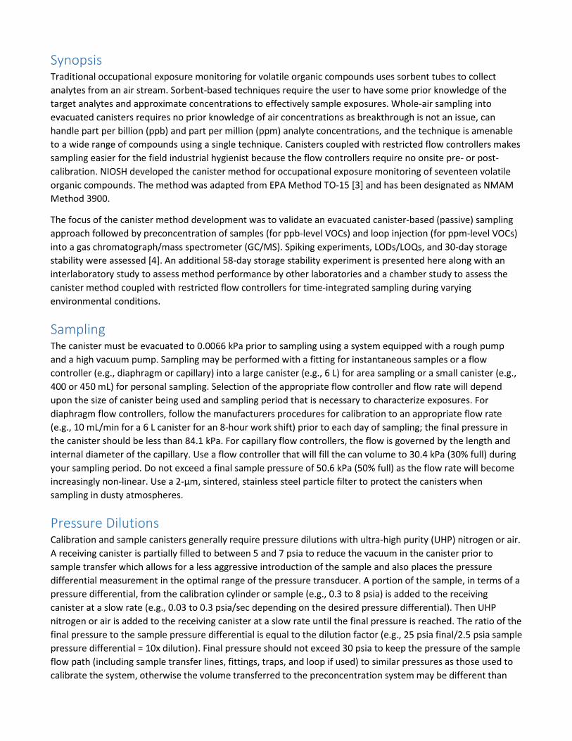
Exposure Limits Table 1. Exposure Limits (ppm) [1, 2]
Substance OSHA TWA
OSHA Peak
NIOSH TWA
NIOSH STEL
mg/m3
per ppm
ethanol 1000 1000 1.89 2-propanol 400 400 500 2.46 acetone 1000 250 2.38 2,3-butanedione 0.005 0.025 3.52 2,3-pentanedione 0.0093 0.031 4.09 2,3-hexanedione 4.67 dichloromethane 25 125 NA (ca) 3.47 trichloromethane 50 2 (60 min) 4.88 hexane 500 50 3.53 benzene 1 5 0.1 (ca) 1 (ca) 3.19 toluene 200 500 100 150 3.77 ethylbenzene 100 100 125 4.34 o-xylene 100 100 150 4.34 m-xylene 100 100 150 4.34 p-xylene 100 100 150 4.34 methyl methacrylate 100 100 4.09 α-pinene 5.57 d-limonene 5.57
Note: ca = carcinogen; NA = not applicable
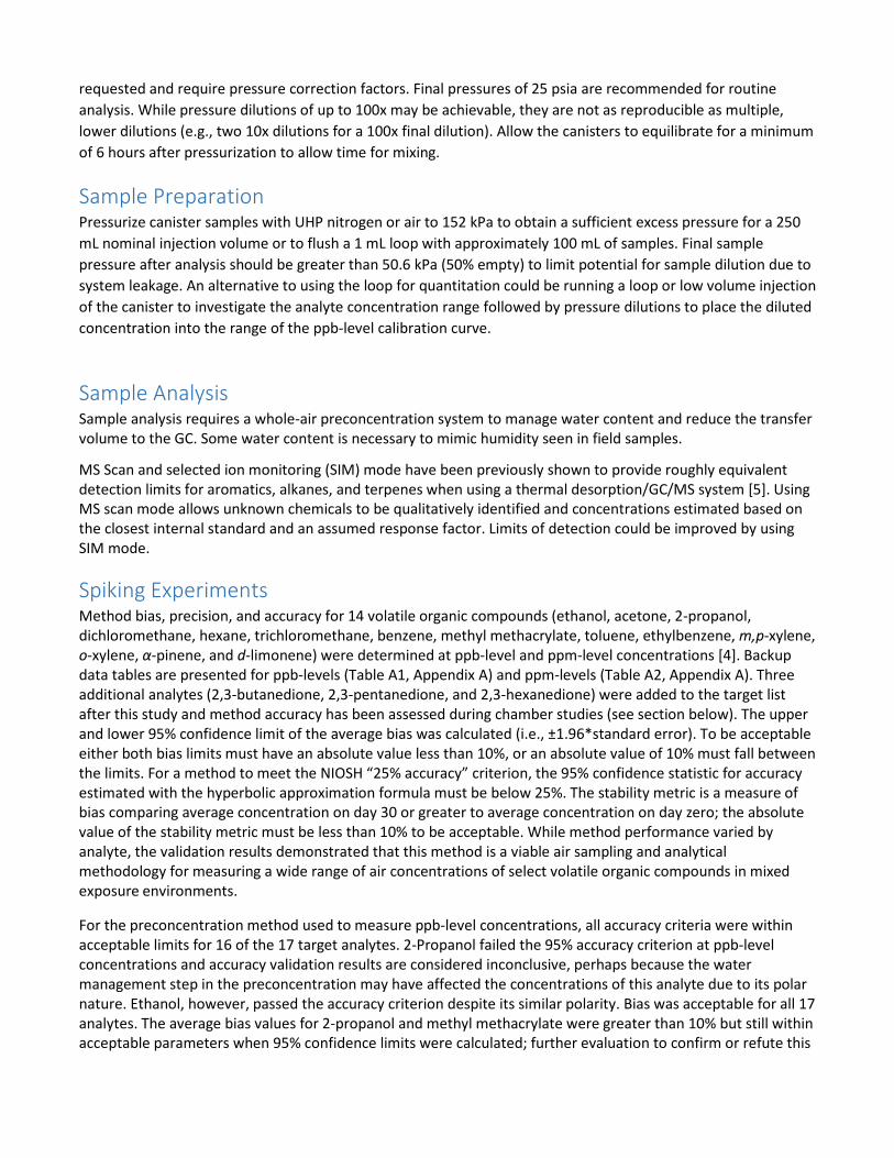
Synopsis Traditional occupational exposure monitoring for volatile organic compounds uses sorbent tubes to collect analytes from an air stream. Sorbent-based techniques require the user to have some prior knowledge of the target analytes and approximate concentrations to effectively sample exposures. Whole-air sampling into evacuated canisters requires no prior knowledge of air concentrations as breakthrough is not an issue, can handle part per billion (ppb) and part per million (ppm) analyte concentrations, and the technique is amenable to a wide range of compounds using a single technique. Canisters coupled with restricted flow controllers makes sampling easier for the field industrial hygienist because the flow controllers require no onsite pre- or post- calibration. NIOSH developed the canister method for occupational exposure monitoring of seventeen volatile organic compounds. The method was adapted from EPA Method TO-15 [3] and has been designated as NMAM Method 3900.
The focus of the canister method development was to validate an evacuated canister-based (passive) sampling approach followed by preconcentration of samples (for ppb-level VOCs) and loop injection (for ppm-level VOCs) into a gas chromatograph/mass spectrometer (GC/MS). Spiking experiments, LODs/LOQs, and 30-day storage stability were assessed [4]. An additional 58-day storage stability experiment is presented here along with an interlaboratory study to assess method performance by other laboratories and a chamber study to assess the canister method coupled with restricted flow controllers for time-integrated sampling during varying environmental conditions.
Sampling The canister must be evacuated to 0.0066 kPa prior to sampling using a system equipped with a rough pump and a high vacuum pump. Sampling may be performed with a fitting for instantaneous samples or a flow controller (e.g., diaphragm or capillary) into a large canister (e.g., 6 L) for area sampling or a small canister (e.g., 400 or 450 mL) for personal sampling. Selection of the appropriate flow controller and flow rate will depend upon the size of canister being used and sampling period that is necessary to characterize exposures. For diaphragm flow controllers, follow the manufacturers procedures for calibration to an appropriate flow rate (e.g., 10 mL/min for a 6 L canister for an 8-hour work shift) prior to each day of sampling; the final pressure in the canister should be less than 84.1 kPa. For capillary flow controllers, the flow is governed by the length and internal diameter of the capillary. Use a flow controller that will fill the can volume to 30.4 kPa (30% full) during your sampling period. Do not exceed a final sample pressure of 50.6 kPa (50% full) as the flow rate will become increasingly non-linear. Use a 2-µm, sintered, stainless steel particle filter to protect the canisters when sampling in dusty atmospheres.
Pressure Dilutions Calibration and sample canisters generally require pressure dilutions with ultra-high purity (UHP) nitrogen or air. A receiving canister is partially filled to between 5 and 7 psia to reduce the vacuum in the canister prior to sample transfer which allows for a less aggressive introduction of the sample and also places the pressure differential measurement in the optimal range of the pressure transducer. A portion of the sample, in terms of a pressure differential, from the calibration cylinder or sample (e.g., 0.3 to 8 psia) is added to the receiving canister at a slow rate (e.g., 0.03 to 0.3 psia/sec depending on the desired pressure differential). Then UHP nitrogen or air is added to the receiving canister at a slow rate until the final pressure is reached. The ratio of the final pressure to the sample pressure differential is equal to the dilution factor (e.g., 25 psia final/2.5 psia sample pressure differential = 10x dilution). Final pressure should not exceed 30 psia to keep the pressure of the sample flow path (including sample transfer lines, fittings, traps, and loop if used) to similar pressures as those used to calibrate the system, otherwise the volume transferred to the preconcentration system may be different than
requested and require pressure correction factors. Final pressures of 25 psia are recommended for routine analysis. While pressure dilutions of up to 100x may be achievable, they are not as reproducible as multiple, lower dilutions (e.g., two 10x dilutions for a 100x final dilution). Allow the canisters to equilibrate for a minimum of 6 hours after pressurization to allow time for mixing.
Sample Preparation Pressurize canister samples with UHP nitrogen or air to 152 kPa to obtain a sufficient excess pressure for a 250 mL nominal injection volume or to flush a 1 mL loop with approximately 100 mL of samples. Final sample pressure after analysis should be greater than 50.6 kPa (50% empty) to limit potential for sample dilution due to system leakage. An alternative to using the loop for quantitation could be running a loop or low volume injection of the canister to investigate the analyte concentration range followed by pressure dilutions to place the diluted concentration into the range of the ppb-level calibration curve.
Sample Analysis Sample analysis requires a whole-air preconcentration system to manage water content and reduce the transfer volume to the GC. Some water content is necessary to mimic humidity seen in field samples.
MS Scan and selected ion monitoring (SIM) mode have been previously shown to provide roughly equivalent detection limits for aromatics, alkanes, and terpenes when using a thermal desorption/GC/MS system [5]. Using MS scan mode allows unknown chemicals to be qualitatively identified and concentrations estimated based on the closest internal standard and an assumed response factor. Limits of detection could be improved by using SIM mode.
Spiking Experiments Method bias, precision, and accuracy for 14 volatile organic compounds (ethanol, acetone, 2-propanol, dichloromethane, hexane, trichloromethane, benzene, methyl methacrylate, toluene, ethylbenzene, m,p-xylene, o-xylene, α-pinene, and d-limonene) were determined at ppb-level and ppm-level concentrations [4]. Backup data tables are presented for ppb-levels (Table A1, Appendix A) and ppm-levels (Table A2, Appendix A). Three additional analytes (2,3-butanedione, 2,3-pentanedione, and 2,3-hexanedione) were added to the target list after this study and method accuracy has been assessed during chamber studies (see section below). The upper and lower 95% confidence limit of the average bias was calculated (i.e., ±1.96*standard error). To be acceptable either both bias limits must have an absolute value less than 10%, or an absolute value of 10% must fall between the limits. For a method to meet the NIOSH “25% accuracy” criterion, the 95% confidence statistic for accuracy estimated with the hyperbolic approximation formula must be below 25%. The stability metric is a measure of bias comparing average concentration on day 30 or greater to average concentration on day zero; the absolute value of the stability metric must be less than 10% to be acceptable. While method performance varied by analyte, the validation results demonstrated that this method is a viable air sampling and analytical methodology for measuring a wide range of air concentrations of select volatile organic compounds in mixed exposure environments.
For the preconcentration method used to measure ppb-level concentrations, all accuracy criteria were within acceptable limits for 16 of the 17 target analytes. 2-Propanol failed the 95% accuracy criterion at ppb-level concentrations and accuracy validation results are considered inconclusive, perhaps because the water management step in the preconcentration may have affected the concentrations of this analyte due to its polar nature. Ethanol, however, passed the accuracy criterion despite its similar polarity. Bias was acceptable for all 17 analytes. The average bias values for 2-propanol and methyl methacrylate were greater than 10% but still within acceptable parameters when 95% confidence limits were calculated; further evaluation to confirm or refute this
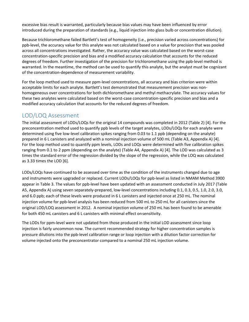
excessive bias result is warranted, particularly because bias values may have been influenced by error introduced during the preparation of standards (e.g., liquid injection into glass bulb or concentration dilution).
Because trichloromethane failed Bartlett’s test of homogeneity (i.e., precision varied across concentrations) for ppb-level, the accuracy value for this analyte was not calculated based on a value for precision that was pooled across all concentrations investigated. Rather, the accuracy value was calculated based on the worst-case concentration-specific precision and bias and a modified accuracy calculation that accounts for the reduced degrees of freedom. Further investigation of the precision for trichloromethane using the ppb-level method is warranted. In the meantime, the method can be used to quantify this analyte, but the analyst must be cognizant of the concentration-dependence of measurement variability.
For the loop method used to measure ppm-level concentrations, all accuracy and bias criterion were within acceptable limits for each analyte. Bartlett’s test demonstrated that measurement precision was non- homogeneous over concentrations for both dichloromethane and methyl methacrylate. The accuracy values for these two analytes were calculated based on the worst-case concentration-specific precision and bias and a modified accuracy calculation that accounts for the reduced degrees of freedom.
LOD/LOQ Assessment The initial assessment of LODs/LOQs for the original 14 compounds was completed in 2012 (Table 2) [4]. For the preconcentration method used to quantify ppb levels of the target analytes, LODs/LOQs for each analyte were determined using five low-level calibration spikes ranging from 0.03 to 1.1 ppb (depending on the analyte) prepared in 6 L canisters and analyzed with a nominal injection volume of 500 mL (Table A3, Appendix A) [4]. For the loop method used to quantify ppm levels, LODs and LOQs were determined with five calibration spikes ranging from 0.1 to 2 ppm (depending on the analyte) (Table A4, Appendix A) [4]. The LOD was calculated as 3 times the standard error of the regression divided by the slope of the regression, while the LOQ was calculated as 3.33 times the LOD [6].
LODs/LOQs have continued to be assessed over time as the condition of the instruments changed due to age and instruments were upgraded or replaced. Current LODs/LOQs for ppb-level as listed in NMAM Method 3900 appear in Table 3. The values for ppb-level have been updated with an assessment conducted in July 2017 (Table A5, Appendix A) using seven separately-prepared, low-level concentrations including 0.1, 0.3, 0.5, 1.0, 2.0, 3.0, and 6.0 ppb; each of these levels were produced in 6 L canisters and injected once at 250 mL. The nominal injection volume for ppb-level analysis has been reduced from 500 mL to 250 mL for all canisters since the original LOD/LOQ assessment in 2012. A nominal injection volume of 250 mL has been found to be amenable for both 450 mL canisters and 6 L canisters with minimal effect on sensitivity.
The LODs for ppm-level were not updated from those produced in the initial LOD assessment since loop injection is fairly uncommon now. The current recommended strategy for higher concentration samples is pressure dilutions into the ppb-level calibration range or loop injection with a dilution factor correction for volume injected onto the preconcentrator compared to a nominal 250 mL injection volume.
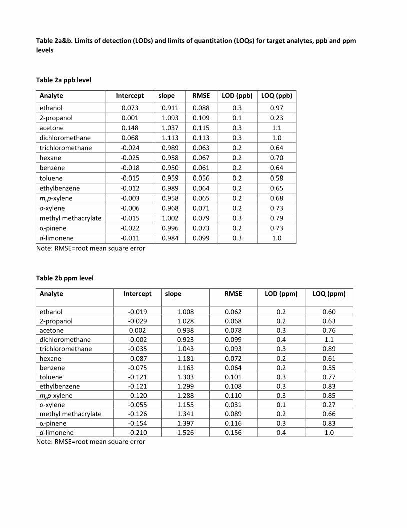
Table 2a&b. Limits of detection (LODs) and limits of quantitation (LOQs) for target analytes, ppb and ppm levels
Table 2a ppb level
Analyte Intercept slope RMSE LOD (ppb) LOQ (ppb)
ethanol 0.073 0.911 0.088 0.3 0.97 2-propanol 0.001 1.093 0.109 0.1 0.23 acetone 0.148 1.037 0.115 0.3 1.1 dichloromethane 0.068 1.113 0.113 0.3 1.0 trichloromethane -0.024 0.989 0.063 0.2 0.64 hexane -0.025 0.958 0.067 0.2 0.70 benzene -0.018 0.950 0.061 0.2 0.64 toluene -0.015 0.959 0.056 0.2 0.58 ethylbenzene -0.012 0.989 0.064 0.2 0.65 m,p-xylene -0.003 0.958 0.065 0.2 0.68 o-xylene -0.006 0.968 0.071 0.2 0.73 methyl methacrylate -0.015 1.002 0.079 0.3 0.79 α-pinene -0.022 0.996 0.073 0.2 0.73 d-limonene -0.011 0.984 0.099 0.3 1.0
Note: RMSE=root mean square error
Table 2b ppm level
Analyte Intercept slope RMSE LOD (ppm) LOQ (ppm)
ethanol -0.019 1.008 0.062 0.2 0.60 2-propanol -0.029 1.028 0.068 0.2 0.63 acetone 0.002 0.938 0.078 0.3 0.76 dichloromethane -0.002 0.923 0.099 0.4 1.1 trichloromethane -0.035 1.043 0.093 0.3 0.89 hexane -0.087 1.181 0.072 0.2 0.61 benzene -0.075 1.163 0.064 0.2 0.55 toluene -0.121 1.303 0.101 0.3 0.77 ethylbenzene -0.121 1.299 0.108 0.3 0.83 m,p-xylene -0.120 1.288 0.110 0.3 0.85 o-xylene -0.055 1.155 0.031 0.1 0.27 methyl methacrylate -0.126 1.341 0.089 0.2 0.66 α-pinene -0.154 1.397 0.116 0.3 0.83 d-limonene -0.210 1.526 0.156 0.4 1.0
Note: RMSE=root mean square error
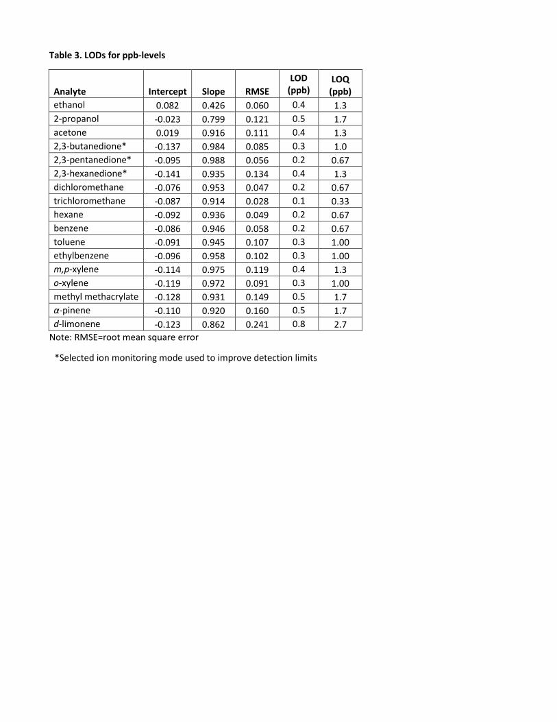
Table 3. LODs for ppb-levels
Analyte
Intercept
Slope
RMSE
LOD (ppb)
LOQ (ppb)
ethanol 0.082 0.426 0.060 0.4 1.3 2-propanol -0.023 0.799 0.121 0.5 1.7 acetone 0.019 0.916 0.111 0.4 1.3 2,3-butanedione* -0.137 0.984 0.085 0.3 1.0 2,3-pentanedione* -0.095 0.988 0.056 0.2 0.67 2,3-hexanedione* -0.141 0.935 0.134 0.4 1.3 dichloromethane -0.076 0.953 0.047 0.2 0.67 trichloromethane -0.087 0.914 0.028 0.1 0.33 hexane -0.092 0.936 0.049 0.2 0.67 benzene -0.086 0.946 0.058 0.2 0.67 toluene -0.091 0.945 0.107 0.3 1.00 ethylbenzene -0.096 0.958 0.102 0.3 1.00 m,p-xylene -0.114 0.975 0.119 0.4 1.3 o-xylene -0.119 0.972 0.091 0.3 1.00 methyl methacrylate -0.128 0.931 0.149 0.5 1.7 α-pinene -0.110 0.920 0.160 0.5 1.7 d-limonene -0.123 0.862 0.241 0.8 2.7
Note: RMSE=root mean square error
*Selected ion monitoring mode used to improve detection limits
Storage Stability Testing Sample storage stability at room temperature was assessed for 14 analytes at 5 ppb and 0.6 ppm over a period of 30 days [4]. For the 5 ppb concentration, a total of twelve 6 L canisters were stored and analyzed repeatedly on days zero, 7, 14, 21, and 30. For the 0.6 ppm concentration, 30 canisters were generated and analyzed only once according to the following schedule: 12 canisters on day zero, six canisters on day 7, and three canisters each on days 14, 21, and 30. The stability metric is bias comparing average concentration on day 30 to average concentration on day zero; the absolute value of the stability metric must be less than 0.10 to be acceptable per NIOSH guidance [6]. If the analyte is not stable for 30 days, the method is still acceptable as long as a shorter stability time is confirmed.
All 14 analytes at ppb-level were stable (i.e., less than 10% change) over a period of 30 days (Table A6, Appendix A). All 14 analytes at ppm-levels were stable for 30 days, except α-pinene and d-limonene, which remained stable for 21 days (Table A7, Appendix A). The shorter acceptable storage time for α-pinene and d-limonene may be due to losses from chemical reactions with other components of canister contents, particularly oxidizing species such as ozone or hydroxyl and nitrate radicals naturally found in indoor air [7, 8].
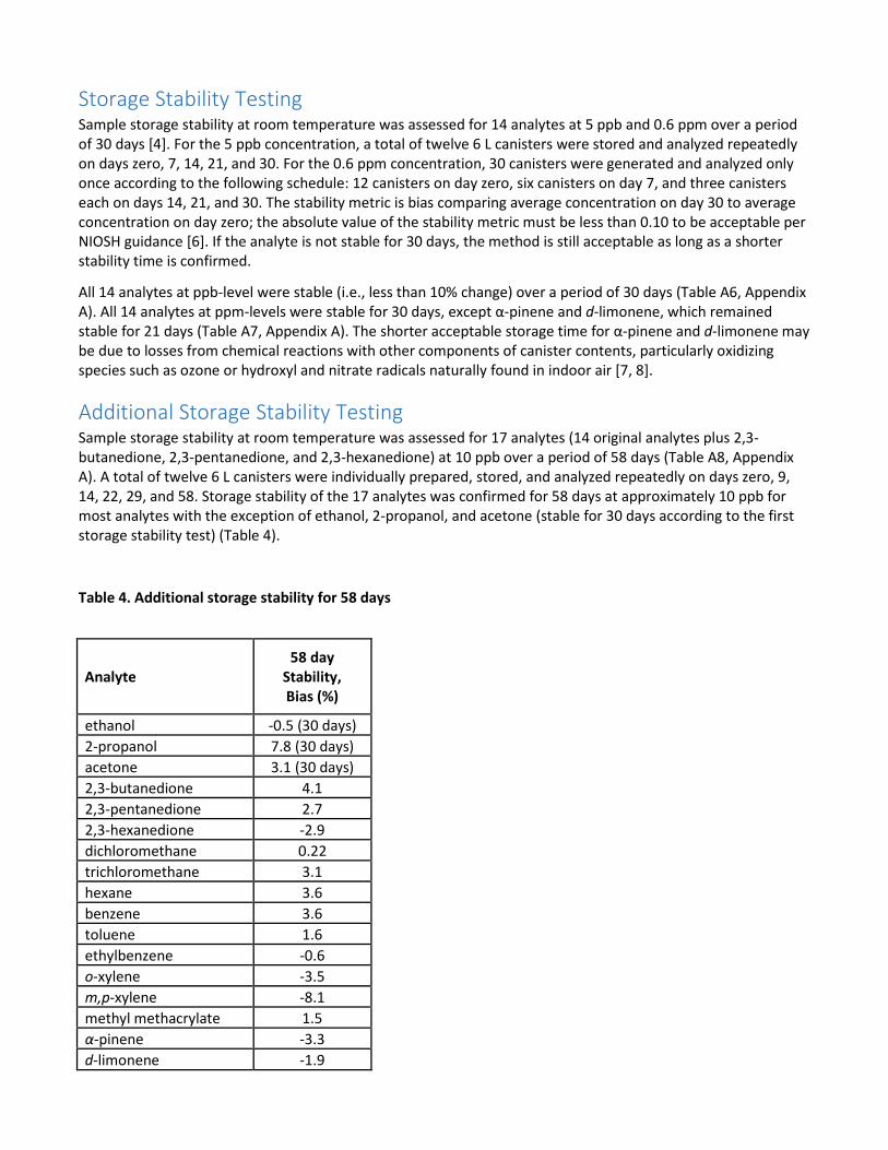
Additional Storage Stability Testing Sample storage stability at room temperature was assessed for 17 analytes (14 original analytes plus 2,3- butanedione, 2,3-pentanedione, and 2,3-hexanedione) at 10 ppb over a period of 58 days (Table A8, Appendix A). A total of twelve 6 L canisters were individually prepared, stored, and analyzed repeatedly on days zero, 9, 14, 22, 29, and 58. Storage stability of the 17 analytes was confirmed for 58 days at approximately 10 ppb for most analytes with the exception of ethanol, 2-propanol, and acetone (stable for 30 days according to the first storage stability test) (Table 4).
Table 4. Additional storage stability for 58 days
Analyte
58 day Stability, Bias (%)
ethanol -0.5 (30 days) 2-propanol 7.8 (30 days) acetone 3.1 (30 days) 2,3-butanedione 4.1 2,3-pentanedione 2.7 2,3-hexanedione -2.9 dichloromethane 0.22 trichloromethane 3.1 hexane 3.6 benzene 3.6 toluene 1.6 ethylbenzene -0.6 o-xylene -3.5 m,p-xylene -8.1 methyl methacrylate 1.5 α-pinene -3.3 d-limonene -1.9
Dynamically-generated Samples: Chamber Studies Canister method was challenged using alpha-diketones in chamber studies under varying environmental conditions to assess sampling and analytical accuracy following ASTM D6246 [9]. The following conditions were assessed: temperature, humidity, wind speed, and concentration. Additional VOCs (ethanol, acetone, 2- propanol, dichloromethane, trichloromethane, methyl methacrylate, hexane, benzene, toluene, o-xylene, m,p- xylene, α-pinene, d-limonene) were present during low and high humidity trials to assess the effect of humidity on method performance for these analytes. Bias pulse tests were performed to assess the bias associated with a known drop in flow rate (~13% over the sampling period) for capillary flow controllers. Flow rate bias (bias pulse) was assessed using the difference in measurements for peak exposures occurring at the beginning and end of the sampling period. Tests were also performed to assess inter-day and inter-sampler variation. A dynamic volatile organic compound generation and sampling system was used to produce known concentrations of challenge agents in a glass sampling chamber with 18 sampling ports. The system was placed in a large walk- in environmental control chamber to regulate temperature. Capillary flow controllers were constructed using Swagelok connections and deactivated fused-silica tubing to collect air samples at 15 mL/min for 15 minutes into a 450 mL canister. Canisters were pressurized with ultra-high purity nitrogen and analyzed using an autosampler/preconcentrator system attached to a gas chromatograph/mass spectrometer. Results were corrected for pressure dilution and compared to a theoretical concentration calculated from flow dilution of the certified gas standard used in the generation system. Accuracy was calculated for each target analyte for all conditions combined. Variance estimates for each factor influencing accuracy were used to apportion the relative influence of each test condition on the overall performance of the method. Upper confidence limits on accuracy (A95) were below 0.25 for all analytes: 0.085 for 2,3-butanedione, 0.142 for 2,3-pentanedione, and 0.194 for 2,3-hexanedione. Overall precision was largest for 2,3-hexanedione at 0.061 with 27.4% of the total variance due to inter-day variability. The peak exposure condition accounted for less than 6% of the variability regardless of analyte, meaning the known drop in flow rate from the capillary flow controller did not adversely affect air sampling. Canister method is a reliable, robust sampling and analytical method that may be used for a variety of analytes (e.g., C1 to C10) under varying environmental conditions.
Chamber Study Methods Chamber Study protocol The VOC generation system was constructed in a large walk-in environmental chamber (Nor-Lake Scientific, Hudson, WI) to control temperature close to the test condition. The test chamber was a glass cylinder with nine ports for sampling (replica of OSHA test chamber). VOC concentration homogeneity was assessed by sampling silica gel sorbent tubes (SKC cat no. 226-183) at each port. Tubes were analyzed using a modified OSHA 1016 method (mass spectrometry instead of flame ionization detection) [10]. Variability between ports was 4.1% for 2,3-butanedione, 4.4% for 2,3-pentanedione, and 3.9% for 2,3-hexanedione. The temperature, humidity, and flow rate of the dilution air to test chamber was controlled by a Miller-Nelson unit (Model HCS-501, Assay Technology, Livermore, CA). The VOC concentration was generated by flow dilution of a certified calibration gas cylinder at approximately 2 ppm (±5% analytical accuracy) (Linde Spectra Environmental Gases, Alpha, NJ) using a mass flow controller (Aalborg, Orangeburg, NY). Blank samples collected prior to conducting the studies ensured system cleanliness. No alpha-diketones were detected above the MDL (0.01 µg/sample which is 0.95 ppb 2,3-butanedione for a 15 minute air sample collected at 200 mL/min). Trials were conducted at a constant concentration. For the bias pulse experiments, the sampler was attached to the test chamber for 1 out of 15 minutes at the beginning or end of the sampling period. For the rest of the trial, the sampler was placed in a tedlar bag filled with UHP nitrogen gas.
NIOSH draft canister method was used to analyze canister samples. Briefly, canisters were pressurized to 1.5 times atmospheric pressure with UHP nitrogen prior to analysis on an Entech 7200/7032
preconcentrator/autosampler (Simi Valley, CA) attached to an Agilent 6890/5975 gas chromatograph/mass spectrometer. Canister injection volume was 25, 50, or 250 mL adjusted to produce a mass loading on the column within the calibration curve. Calibration curve dynamic range was from 0.2 to 40 ppb. Canisters were allowed to equilibrate for at least three hours prior to analysis. Each analyte response was referenced to an internal standard response and compared to a calibration curve. Internal standards were bromochloromethane, 1,4-difluorobenzene, chlorobenzene-d5 at 25 ppb with a 50 mL loading on the preconcentrator module prior to sample loading. A pressure dilution factor was applied to the measure concentration for final reporting. Bias was calculated as the difference between the final result and the flow dilution theoretical value (assuming no error in the theoretical value). Bartley calculation was employed for point estimate accuracy and confidence limits on accuracy [11]. Variance estimates for each trial as well as aggregate bias and overall inter-sampler variation were used to apportion the relative percentage effect (squared error over total squared error) of each of the conditions on method performance. Bias pulse was calculated as the difference between the beginning and end pulse measurements divided by the sum of the measurements [9].
Chamber Study Design The effect of environmental conditions on method performance in terms of bias and precision were assessed using different trials based on ASTM D6246 [9]. The experimental trials included humidity, wind speed, concentration, inter-day, beginning pulse, and end pulse (Table 5). High wind speed was difficult to achieve with the VOC generation system, so a low wind speed (0.009 m/s) was substituted. The rest of the trials were conducted between 0.033 and 0.042 m/s depending on VOC generation needs. Additional VOCs (ethanol, acetone, 2-propanol, dichloromethane, trichloromethane, methyl methacrylate, hexane, benzene, toluene, o- xylene, m,p-xylene, α-pinene, d-limonene) were present during low and high humidity trials at the same nominal concentration as the alpha-diketones (400 ppb). Trial sample sizes ranged from 5 to 12 due to constraints on the analytical system at the time of analysis (i.e., other projects like NIOSH Health Hazard Evaluation samples took precedence) and lost samples or outlier results. Lost samples were due to low liquid nitrogen pressure during analysis causing a failed injection. For the high humidity trial, 12 samples were collected but one was lost; one was visually identified as an outlier (bias -0.33 for 2,3-butanedione, -0.64 for 2,3-pentanedione, and -0.81 for 2,3-hexanedione) and removed. For the high temperature trial, 6 samples were collected; one was visually identified as an outlier (bias -0.18 for 2,3-butanedione, -0.39 for 2,3-pentanedione, and -0.79 for 2,3- hexanedione) and removed. For the low humidity trial, 6 samples were collected; one was visually identified as an outlier (bias -0.01 for 2,3-butanedione, -0.22 for 2,3-pentanedione, and -0.37 for 2,3-hexanedione) and removed. For the end pulse trial, 9 samples were collected; one sample was lost.
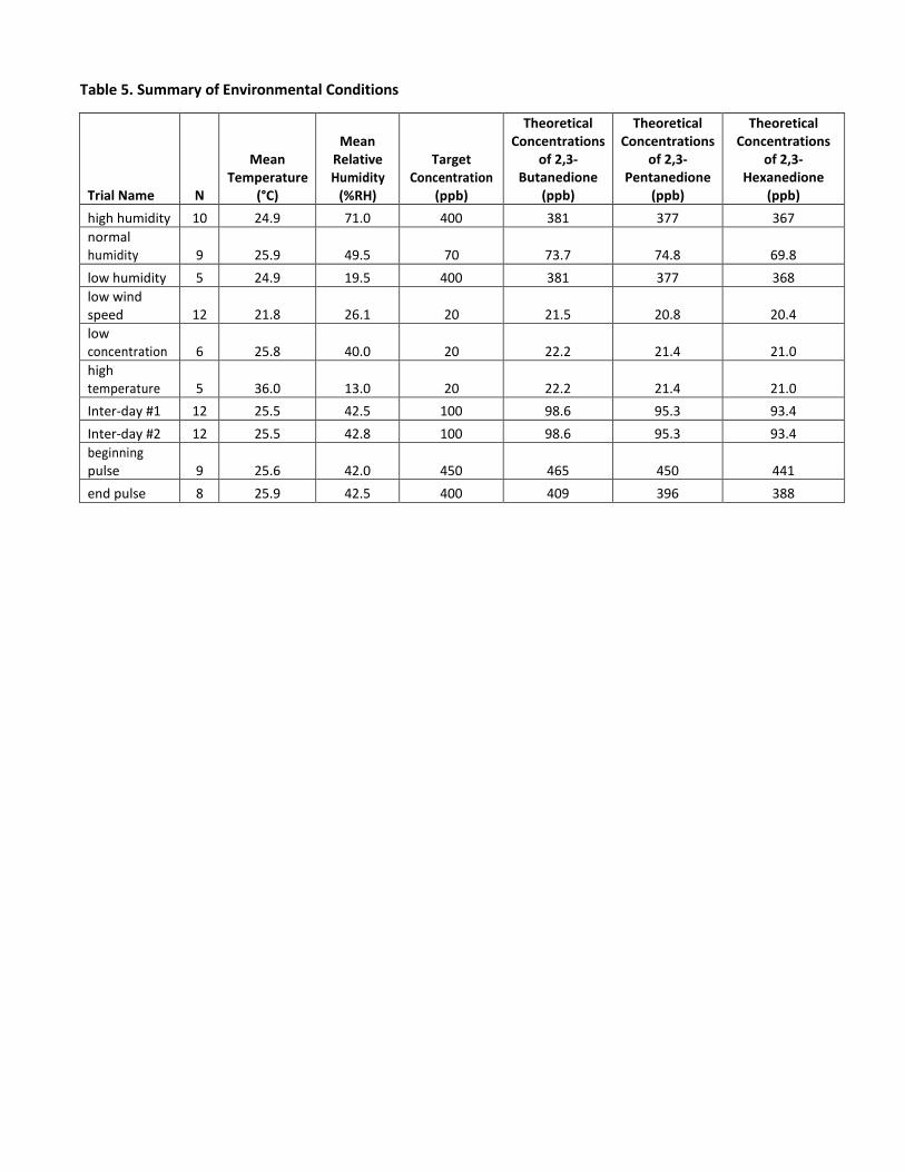
Table 5. Summary of Environmental Conditions
Trial Name
N
Mean Temperature
(°C)
Mean
Relative Humidity
(%RH)
Target Concentration
(ppb)
Theoretical Concentrations
of 2,3- Butanedione
(ppb)
Theoretical Concentrations
of 2,3- Pentanedione
(ppb)
Theoretical Concentrations
of 2,3- Hexanedione
(ppb) high humidity 10 24.9 71.0 400 381 377 367 normal humidity
9
25.9
49.5
70
73.7
74.8
69.8
low humidity 5 24.9 19.5 400 381 377 368 low wind speed
12
21.8
26.1
20
21.5
20.8
20.4
low concentration
6
25.8
40.0
20
22.2
21.4
21.0
high temperature
5
36.0
13.0
20
22.2
21.4
21.0
Inter-day #1 12 25.5 42.5 100 98.6 95.3 93.4 Inter-day #2 12 25.5 42.8 100 98.6 95.3 93.4 beginning pulse
9
25.6
42.0
450
465
450
441
end pulse 8 25.9 42.5 400 409 396 388
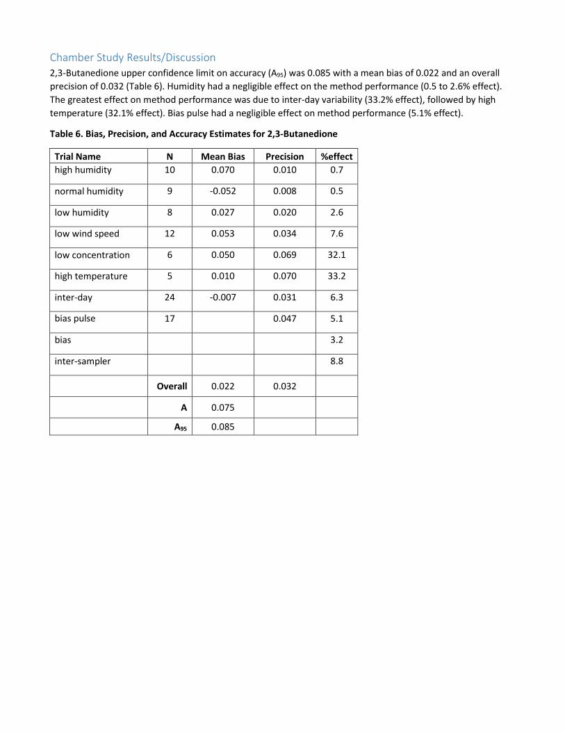
Chamber Study Results/Discussion 2,3-Butanedione upper confidence limit on accuracy (A95) was 0.085 with a mean bias of 0.022 and an overall precision of 0.032 (Table 6). Humidity had a negligible effect on the method performance (0.5 to 2.6% effect). The greatest effect on method performance was due to inter-day variability (33.2% effect), followed by high temperature (32.1% effect). Bias pulse had a negligible effect on method performance (5.1% effect).
Table 6. Bias, Precision, and Accuracy Estimates for 2,3-Butanedione
Trial Name N Mean Bias Precision %effect high humidity 10 0.070 0.010 0.7
normal humidity 9 -0.052 0.008 0.5
low humidity 8 0.027 0.020 2.6
low wind speed 12 0.053 0.034 7.6
low concentration 6 0.050 0.069 32.1
high temperature 5 0.010 0.070 33.2
inter-day 24 -0.007 0.031 6.3
bias pulse 17 0.047 5.1
bias 3.2
inter-sampler 8.8
Overall 0.022 0.032
A 0.075
A95 0.085
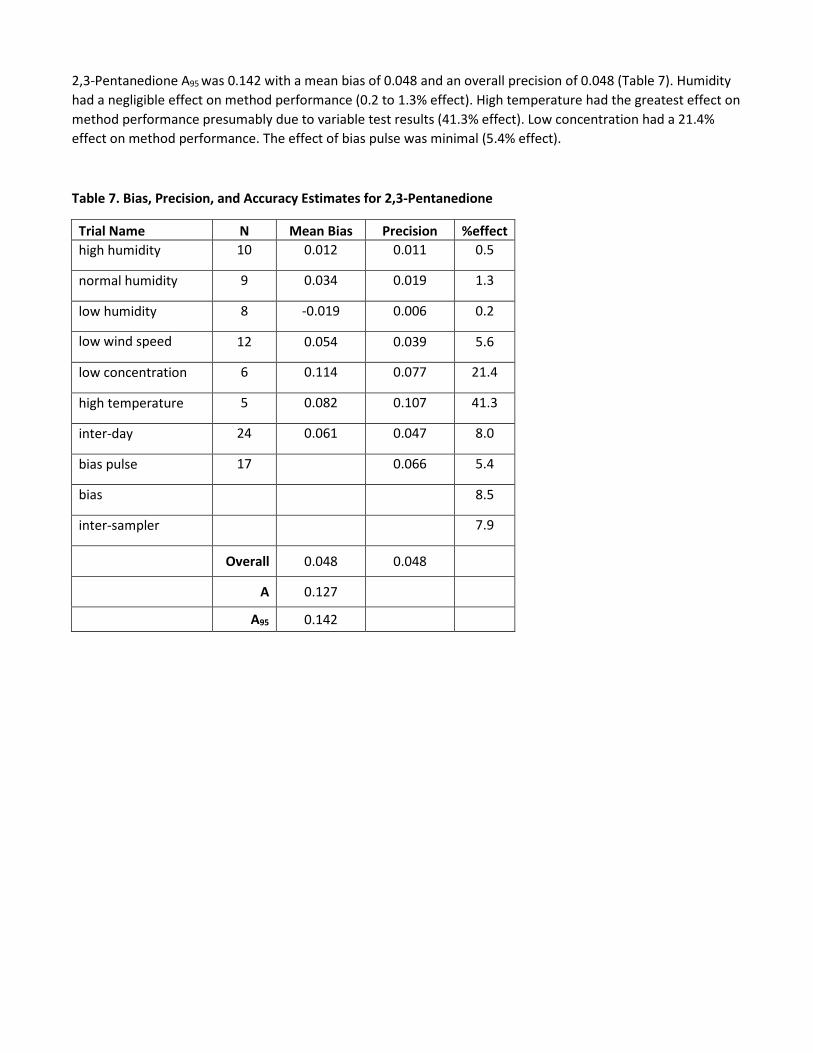
2,3-Pentanedione A95 was 0.142 with a mean bias of 0.048 and an overall precision of 0.048 (Table 7). Humidity had a negligible effect on method performance (0.2 to 1.3% effect). High temperature had the greatest effect on method performance presumably due to variable test results (41.3% effect). Low concentration had a 21.4% effect on method performance. The effect of bias pulse was minimal (5.4% effect).
Table 7. Bias, Precision, and Accuracy Estimates for 2,3-Pentanedione
Trial Name N Mean Bias Precision %effect high humidity 10 0.012 0.011 0.5
normal humidity 9 0.034 0.019 1.3
low humidity 8 -0.019 0.006 0.2
low wind speed 12 0.054 0.039 5.6
low concentration 6 0.114 0.077 21.4
high temperature 5 0.082 0.107 41.3
inter-day 24 0.061 0.047 8.0
bias pulse 17 0.066 5.4
bias 8.5
inter-sampler 7.9
Overall 0.048 0.048
A 0.127
A95 0.142
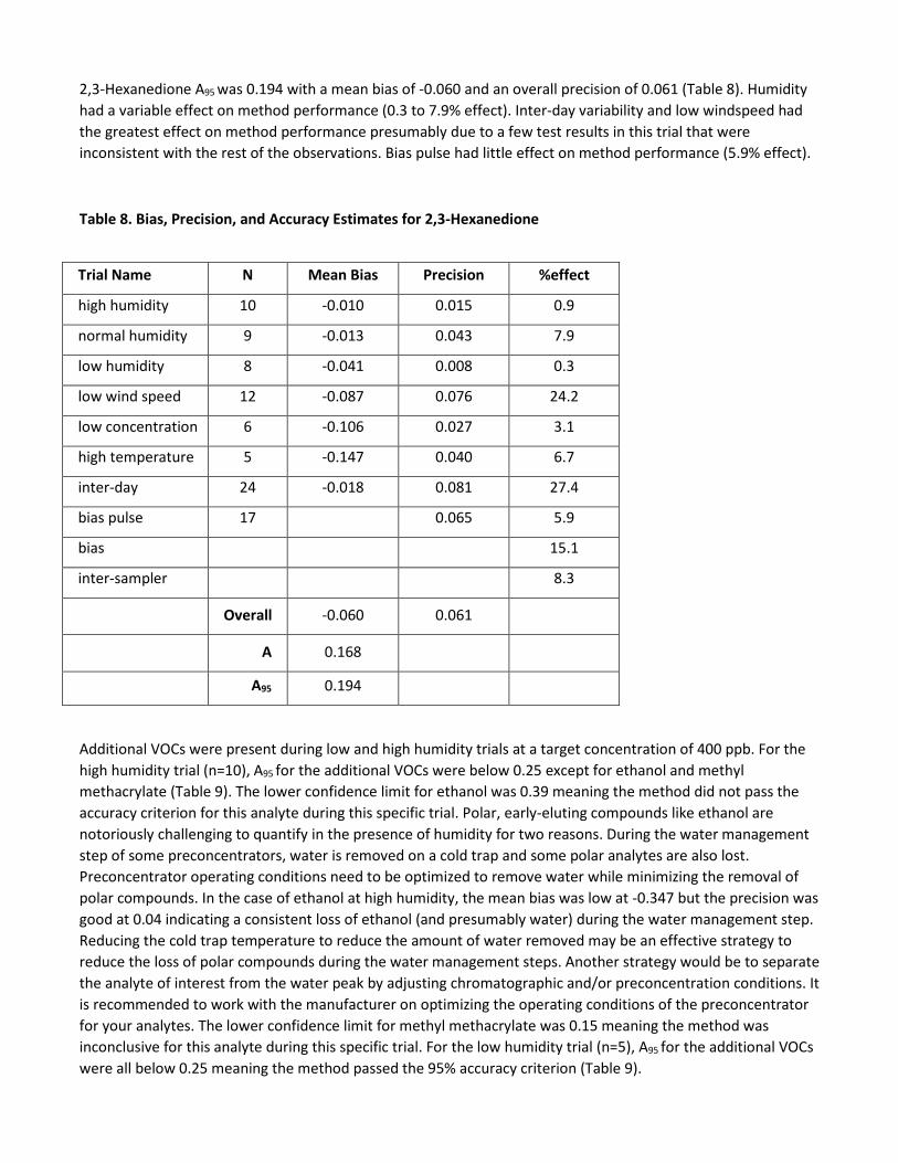
2,3-Hexanedione A95 was 0.194 with a mean bias of -0.060 and an overall precision of 0.061 (Table 8). Humidity had a variable effect on method performance (0.3 to 7.9% effect). Inter-day variability and low windspeed had the greatest effect on method performance presumably due to a few test results in this trial that were inconsistent with the rest of the observations. Bias pulse had little effect on method performance (5.9% effect).
Table 8. Bias, Precision, and Accuracy Estimates for 2,3-Hexanedione
Trial Name N Mean Bias Precision %effect
high humidity 10 -0.010 0.015 0.9
normal humidity 9 -0.013 0.043 7.9
low humidity 8 -0.041 0.008 0.3
low wind speed 12 -0.087 0.076 24.2
low concentration 6 -0.106 0.027 3.1
high temperature 5 -0.147 0.040 6.7
inter-day 24 -0.018 0.081 27.4
bias pulse 17 0.065 5.9
bias 15.1
inter-sampler 8.3
Overall -0.060 0.061
A 0.168
A95 0.194
Additional VOCs were present during low and high humidity trials at a target concentration of 400 ppb. For the high humidity trial (n=10), A95 for the additional VOCs were below 0.25 except for ethanol and methyl methacrylate (Table 9). The lower confidence limit for ethanol was 0.39 meaning the method did not pass the accuracy criterion for this analyte during this specific trial. Polar, early-eluting compounds like ethanol are notoriously challenging to quantify in the presence of humidity for two reasons. During the water management step of some preconcentrators, water is removed on a cold trap and some polar analytes are also lost. Preconcentrator operating conditions need to be optimized to remove water while minimizing the removal of polar compounds. In the case of ethanol at high humidity, the mean bias was low at -0.347 but the precision was good at 0.04 indicating a consistent loss of ethanol (and presumably water) during the water management step. Reducing the cold trap temperature to reduce the amount of water removed may be an effective strategy to reduce the loss of polar compounds during the water management steps. Another strategy would be to separate the analyte of interest from the water peak by adjusting chromatographic and/or preconcentration conditions. It is recommended to work with the manufacturer on optimizing the operating conditions of the preconcentrator for your analytes. The lower confidence limit for methyl methacrylate was 0.15 meaning the method was inconclusive for this analyte during this specific trial. For the low humidity trial (n=5), A95 for the additional VOCs were all below 0.25 meaning the method passed the 95% accuracy criterion (Table 9).
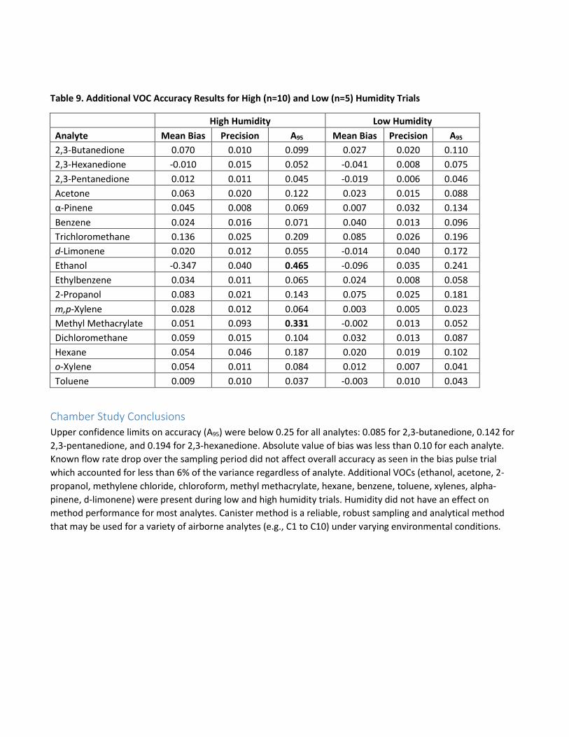
Table 9. Additional VOC Accuracy Results for High (n=10) and Low (n=5) Humidity Trials
High Humidity Low Humidity Analyte Mean Bias Precision A95 Mean Bias Precision A95
2,3-Butanedione 0.070 0.010 0.099 0.027 0.020 0.110 2,3-Hexanedione -0.010 0.015 0.052 -0.041 0.008 0.075 2,3-Pentanedione 0.012 0.011 0.045 -0.019 0.006 0.046 Acetone 0.063 0.020 0.122 0.023 0.015 0.088 α-Pinene 0.045 0.008 0.069 0.007 0.032 0.134 Benzene 0.024 0.016 0.071 0.040 0.013 0.096 Trichloromethane 0.136 0.025 0.209 0.085 0.026 0.196 d-Limonene 0.020 0.012 0.055 -0.014 0.040 0.172 Ethanol -0.347 0.040 0.465 -0.096 0.035 0.241 Ethylbenzene 0.034 0.011 0.065 0.024 0.008 0.058 2-Propanol 0.083 0.021 0.143 0.075 0.025 0.181 m,p-Xylene 0.028 0.012 0.064 0.003 0.005 0.023 Methyl Methacrylate 0.051 0.093 0.331 -0.002 0.013 0.052 Dichloromethane 0.059 0.015 0.104 0.032 0.013 0.087 Hexane 0.054 0.046 0.187 0.020 0.019 0.102 o-Xylene 0.054 0.011 0.084 0.012 0.007 0.041 Toluene 0.009 0.010 0.037 -0.003 0.010 0.043
Chamber Study Conclusions Upper confidence limits on accuracy (A95) were below 0.25 for all analytes: 0.085 for 2,3-butanedione, 0.142 for 2,3-pentanedione, and 0.194 for 2,3-hexanedione. Absolute value of bias was less than 0.10 for each analyte. Known flow rate drop over the sampling period did not affect overall accuracy as seen in the bias pulse trial which accounted for less than 6% of the variance regardless of analyte. Additional VOCs (ethanol, acetone, 2- propanol, methylene chloride, chloroform, methyl methacrylate, hexane, benzene, toluene, xylenes, alpha- pinene, d-limonene) were present during low and high humidity trials. Humidity did not have an effect on method performance for most analytes. Canister method is a reliable, robust sampling and analytical method that may be used for a variety of airborne analytes (e.g., C1 to C10) under varying environmental conditions.

Interlaboratory Study (ILS) Authors: Ryan F. LeBouf, H. Amy Feng, and Stanley A. Shulman
An evacuated canister method for sampling and analysis of select volatile organic compounds was developed at the NIOSH Respiratory Health Division Organic Laboratory in Morgantown, WV. An inter-laboratory study was conducted to assess repeatability and reproducibility of the test method prior to incorporation of the method in the NIOSH Manual of Analytical Methods. Nine laboratories completed the study on the test mix containing 17 analytes: ethanol, 2-propanol (isopropyl alcohol), acetone, dichloromethane (methylene chloride), trichloromethane (chloroform), hexane, 2,3-butanedione, 2,3-pentanedione, 2,3-hexanedione, benzene, toluene, ethylbenzene, o-xylene, m,p-xylene, methyl methacrylate, α-pinene, and d-limonene. Blind spiked test samples were shipped to each laboratory. Spikes consisted of two concentration ranges, three nominal levels, and three replicates per combination (n=18 samples per laboratory, except for the reference laboratory who analyzed between three and six replicates). For quality control, two samples containing UHP nitrogen were included as laboratory blanks for each round. Spikes were produced in batches to accommodate each round which included one to three laboratories at the same time depending on laboratory availability and feasibility in sample preparation. Reference canisters were produced with each batch and analyzed in-house to ensure spike generation was acceptable prior to shipment. Precision estimates for repeatability ranged from 0.04 to 0.55 at ppb concentrations and from 0.10 to 0.47 for ppm concentrations over all analytes and nominal levels. Precision estimates for reproducibility ranged from 0.10 to 0.62 at ppb concentrations and from 0.19 to 0.58 at ppm concentrations, depending on analyte and nominal levels. Plots of h and k statistics which measure the between- and within-laboratory consistency indicated inconsistencies with reported results from laboratories 5, 6, and 7. All results were retained due to the low number of participating laboratories. Training on pressure dilution techniques and preconcentration systems as well as proficiency testing should be periodically conducted to ensure operating laboratories maintain optimal canister method performance.
ILS Methods ILS Participating Laboratories The canister method was based on a validation study by a single laboratory [4]. Laboratories were recruited from American Industrial Hygiene Association (AIHA)-accredited or National Environmental Laboratory Accreditation Program (NELAP)-accredited laboratories which had the experience and equipment necessary to analyze canister samples. Ten laboratories were engaged with one lost due to attrition. Laboratories were scheduled together to receive the test samples when possible to reduce the number of reference samples needed for quality assurance. Laboratories were numbered 0 to 8 for anonymity at aggregation, where laboratory 0 was the reference laboratory. Individual laboratory results were given to each participating laboratory upon completion. A protocol, a draft NMAM method, and a results template were provided by email to each participating laboratory along with a certified gas standard to construct a preliminary calibration curve at least two weeks prior to receiving the test samples.
Laboratories conducted the study between September 2013 and August 2014 with one laboratory (laboratory 6) repeating the study in October 2015 due to poor performance with biases ranging from -1.0 to 2.75, attributable to instrument variability and exceeding the recommended sample storage time (30 days). After the ILS study, sample storage stability was demonstrated to be 58 days for most analytes.
For the most part, contract laboratories were equipped to analyze canisters using EPA Method TO-15 which is a sensitive method for analyzing ambient air toxics. Analysis of TO-15 canister samples requires the use of a preconcentrator with a large injection volume ranging from 250 to 500 mL. The reference laboratory injected 250 mL for ppb-level samples. Most participating laboratories did not have a loop available for ppm-level analysis necessitating pressure or volume dilutions to decrease instrument mass loading into their ppb-level
quantitation range. The reference laboratory, therefore, used two techniques to assess ppm-level concentrations: nitrogen pressure dilution and loop injection. Since most laboratories performed pressure dilutions (except laboratory 3 which used a 1 mL loop injection), these data are included for ppm-level reference laboratory data (laboratory 0).
ILS Study Design The test method was challenged at two concentration ranges (ppb and ppm) with three nominal levels (low, medium, high) per concentration range. The nominal levels were 5, 10, and 15 ppb and 0.8, 1.3 and 1.7 ppm. Three replicate canisters at each concentration were tested including a set analyzed in-house to assess spike generation. Each canister contained a mixture of 17 analytes. Two laboratory blanks with ultra-high purity nitrogen were shipped with the samples. The first round of testing involved two laboratories and served as a pilot study to identify any issues with the study protocol or method instructions. No issues were revealed during the pilot study.
ILS Spike Preparation PPB-range samples were prepared from a gas standard (Linde, Braddock, PA) using flow dilution with nitrogen or using pressure dilutions with nitrogen. Linde is an ISO 17034-accredited reference material provider. PPM-range samples were prepared using pressure dilutions with nitrogen. Most samples were prepared in 450 mL canisters, except for laboratory three who requested 6 L canisters for ppb-range spikes to enable multiple injections. Two canisters for each laboratory were pressurized with nitrogen for laboratory blanks. Each canister was spiked with all 17 analytes. Example canister data are shown for laboratory 6 at 0.8 ppm in Table 10. Multiple spike batches were required due to canister equipment inventory and logistics in preparation: five spike batches for ppb-level and eight spike batches for ppm-level. Except for the reference laboratory, each laboratory analyzed canisters from just one spike-batch. For ppm-level each lab 1 to 8 analyzed canisters from a different spike-batch. For ppm-level spike batch 6 and 7, the generation procedure was changed from a manifold system that simultaneously produced up to nine canisters at a given concentration to a master cylinder preparation of a given concentration followed by pressure transfers. For ppb-level, laboratories 1 and 2 analyzed canisters from the same batch, and laboratories 3, 4 and 5 analyzed canisters from the same batch. Laboratories 6, 7, and 8 each had their own spike-batches. For the statistical analysis each laboratory except the reference laboratory received three canisters at each of the three ppb levels and three canisters at each of the three ppm levels. The reference laboratory received more for some batches.
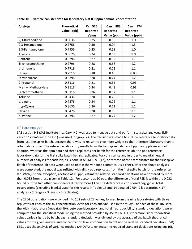
Table 10. Example canister data for laboratory 6 at 0.8 ppm nominal concentration
Analyte Theoretical Value (ppb)
Can 526 Reported
Value
Can 883 Reported Value (ppb)
Can 974 Reported Value (ppb)
2,3-Butanedione 0.8036 0.25 0.56 1.0 2,3-Hexanedione 0.7756 0.30 0.04 1.3 2,3-Pentanedione 0.7956 0.25 0.59 1.0 Acetone 0.8676 0.24 0.53 1.0 Benzene 0.8396 0.27 0.32 1.1 Trichloromethane 0.7796 0.28 0.63 1.2 d-Limonene 0.7716 0.21 0.21 1.1 Ethanol 0.7916 0.18 0.45 0.88 Ethylbenzene 0.8396 0.28 0.24 1.2 2-Propanol 0.8116 0.21 0.55 0.93 Methyl Methacrylate 0.8116 0.24 0.48 0.93 Dichloromethane 0.8116 0.26 0.52 1.1 Toluene 0.8436 0.28 0.28 1.1 α-pinene 0.7876 0.24 0.26 1.1 m,p-Xylene 0.8636 0.26 0.11 1.1 Hexane 0.8476 0.28 0.55 1.1 o-Xylene 0.8396 0.27 0.24 1.2
ILS Data Analysis SAS version 9.3 (SAS Institute Inc., Cary, NC) was used to manage data and perform statistical analyses. JMP version 12 (SAS Institute Inc.) was used for graphics. The decision was made to include reference laboratory data from just one spike-batch, because there was no reason to give more weight to the reference laboratory than to other laboratories. The reference laboratory results from the first spike batches of ppm and ppb were used. In addition, whereas the ppm data had three replicates per batch for the reference lab, the ppb reference laboratory data for the first spike batch had six replicates. For consistency and in order to maintain equal numbers of analyses for each lab, as is done in ASTM E691 [12], only three of the six replicates for the first spike batch of reference lab data were used to obtain the variance estimates. As a check, after the above analyses were completed, the model was refitted with all six ppb replicates from the first spike batch for the reference lab. With just one exception, acetone at 10 ppb, estimated relative standard deviations never differed by more than 0.032 from those given in Table 12. (For acetone at 10 ppb, the difference of total RSD is within the 0.032 bound but the two other components differ by more.) This size difference is considered negligible. Total observations (excluding blanks) used for the results in Tables 13 and 14 equaled 2754 (9 laboratories × 17 analytes × 2 ranges × 3 levels × 3 replicates).
The 2754 observations were divided into 102 sets of 27 values, formed from the nine laboratories with three replicates at each of the six concentration levels for each analyte used in the study. For each of these 102 sets, the within-laboratory (repeatability), between-laboratory, and total (reproducibility) standard deviations were computed for the statistical model using the method provided by ASTM E691. Furthermore, since theoretical values varied slightly by batch, each standard deviation was divided by the average of the batch theoretical values for the given analyte and concentration level combination to obtain the relative standard deviation (RSD). E691 uses the analysis of variance method (ANOVA) to estimate the required standard deviations using eqs (6),

(7), (8), and (10) in ASTM E691. Example calculations of the RSDs are given in Table 11 for benzene at the 0.8 ppm level. The ASTM statistical models do not deal with samples from canisters. However, some discussion of the canister data is presented below.
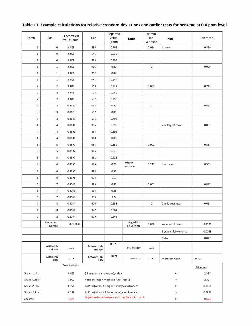
Table 11. Example calculations for relative standard deviations and outlier tests for benzene at 0.8 ppm level
Batch Lab Theoretical Value (ppm) Can
Reported Value (ppm)
NoteWithin
lab variance
Note Lab means
1 0 0.868 895 0.763 0.014 hi mean 0.896
1 0 0.868 546 0.932
1 0 0.868 893 0.993
1 1 0.868 901 0.83 0 0.839
1 1 0.868 902 0.84
1 1 0.868 946 0.847
2 2 0.848 519 0.727 0.002 0.715
2 2 0.848 523 0.666
2 2 0.848 532 0.753
3 3 0.8623 964 0.83 0 0.812
3 3 0.8623 517 0.81
3 3 0.8623 535 0.795
4 4 0.8601 955 0.898 0 2nd largest mean 0.891
4 4 0.8601 534 0.896
4 4 0.8601 968 0.88
5 5 0.8597 953 0.859 0.001 0.888
5 5 0.8597 965 0.876
5 5 0.8597 531 0.928
8 6 0.8396 526 0.27 largest variance
0.217 low mean 0.563
8 6 0.8396 883 0.32
8 6 0.8396 974 1.1
6 7 0.8043 995 0.85 0.001 0.877
6 7 0.8043 534 0.88
6 7 0.8043 533 0.9
7 8 0.8044 906 0.658 0 2nd lowest mean 0.655
7 8 0.8044 947 0.662
7 8 0.8044 979 0.645
theoretical average 0.846044 Avg within
lab variance 0.026 variance of means 0.0146
Between lab variance 0.0058
Stdev 0.077
Within lab std dev 0.16 Between lab
std dev
0.077 Total std dev 0.18
within lab RSD
0.19 between lab RSD
0.09 total RSD 0.211 mean lab mean 0.793
Test Statistics 1% values
Grubbs1,hi = 0.855 (hi mean-mean average)/stdev < 2.387
Grubbs1, low= 1.901 Abs((low mean-mean average)/stdev) < 2.387
Grubbs2, hi= 0.776 6/8*var(without 2 highest mns)/var of means > 0.0851
Grubbs2, low=
Cochran
0.219
0.92
6/8*var(without 2 lowest mns)/var of means
largest variance/variance sum; significant for lab 6
>
>
0.0851
0.573
ASTM E691 was also used to develop h (between-laboratory) and k (within-laboratory) consistency statistics prior to outlier removal. Critical values are 2.23 and -2.23 for h-statistic and 2.09 for k-statistic (from Table 5 of ASTM E691). Data were screened for possible outliers by investigating data points in h,k-plots. Outlier tests were performed for each analyte, concentration level combination for which the total RSD was greater than 0.6, using a two-step removal rule, adapted from ISO 5725 [13]. In step one, the highest and lowest laboratory means were used in separate Grubbs tests for comparison to the two-tailed critical value (2.387, for 9 laboratories, 1% level from Table 5 of ISO 5725, see Table 11 for example calculation). If the critical value was exceeded in either test, then all data from the responsible laboratory were removed (n=51 removed) for the particular analyte, concentration level combination. In step two, if no outliers were removed in step one, an additional Grubb’s test was done by computing the statistic based on the two largest or two lowest laboratory means. If these statistics are less than the 1% critical value (0.0851, for 9 laboratories, from Table 5 of ISO 5725, see Table 11 for example calculation) then all of the data from responsible laboratories were removed (n=24 removed). A total of 2.7% (75/2754) were removed, leaving 2679 data points. After removal, only one analyte, 2,3-Hexanedione at 5 ppb, had total RSD greater than 0.6 (Table 13). Measurements that were removed by this removal rule were not used in subsequent computations of the RSDs, which are shown in Tables 13 and 14. Laboratories with poor performance were contacted regarding these data to investigate potential causes for outlying data.
In the process described above, the aim was not to systematically remove all outliers. The procedure was only applied to analytes with very large total RSDs, those greater than 0.6. The largest RSD was about 1.9. The 75 values mentioned above were taken from 21 different analyte, nominal combinations. For the 18 (of the 21) different ppb-range combinations, the ratio of between-laboratory to within-laboratory RSD was at least 1.55, while for the remaining three ppm-range combinations, two of them had between-laboratory RSDs less than within-laboratory RSD. The bulk of the data suggested that the main reason for the large total RSDs was large between-laboratory variability, for which outliers are identified by the two Grubbs tests. These identified outliers were always outliers larger than the other data. (Recall that the tests are two-sided.) In addition, all except six of the outliers were from two labs which each made some changes to the method instructions (discussed below). After removal, all total RSDs were less than 0.51, with one exception with an RSD greater than 0.6, 2,3-Hexanedione at 5 ppb. Neither Grubbs outlier test gave a significant result. The decision was made not to remove the data. It happens that the Cochran test (from Table 4 of ISO 5725) did identify one outlying laboratory, but removal of that laboratory changed the RSDs by very little.
The above procedure differs somewhat from that in ISO 5725 which suggests that the Cochran test for outliers in within-laboratory variability be used first. It happens that of the 21 different analyte, nominal combinations, 18 had significant results by Cochran’s test. For 15 of these 18, the laboratories with the largest variances were also responsible for the large Grubbs statistics (which included the two ppm analytes for which between RSD was less than within RSD). Thus, by both Grubbs and Cochran tests there were three laboratories for which a different laboratory was identified by the Cochran test than by the Grubbs tests, in which case the within RSD is larger than it would be if the laboratory had been removed. In summary, by the two-step removal rule used here, most of the extremely large outliers were removed by simple application of the rule.
ILS Results/Discussion ILS Blank Canisters Laboratories 5 – 7 reported analyte concentrations in UHP nitrogen blank canisters. The highest blank level reported by laboratory 7 was 19 ppb for m,p-xylene. The same UHP nitrogen tested by the reference laboratory during the same period showed m,p-xylene below the detection limit (<0.28 ppb). Most laboratories reported analyte concentrations in the blanks less than detectable or less than one ppb. No blank corrections were used on reported spike canister results.
l ls
Variation of Spike Batches and Estimation of Bias, Based on Reference Laboratory Canisters It is possible that the estimates in Tables 13 and 14 are larger than they would be if all samples at each concentration level had been collected in a single batch for ppb and a single batch for ppm. Recall that the reference laboratory made measurements in every spike batch, but only the reference laboratory results from the first batch were included in the data used for Tables 13 and 14. If only that laboratory’s data are used and if that laboratory is not overly variable, we would expect that the between batch RSD, would be much smaller than those from the inter-laboratory study results. When a laboratory is used only in one batch and a batch includes only one laboratory, there is no way to know whether the data indicate something about the laboratory or about the batch. This issue makes the data analysis more complicated, as discussed below. Only the reference laboratory data avoid this problem.
The statistical models of interest for measurements (x) of an analyte at a concentration level are given below. These models, for both ppb and ppm (102 data sets with 27 measurements in each set) refer to nine laboratories and three samples per laboratory
M1: xls = μ + a l + bls,
where μ is the true mean of the analyte, al is the difference from the overall mean of laboratory l, and bls is the difference from the lab l mean of the sth sample of lab l. al and bls are normally distributed with means 0, and variances σ2 and σ2 , respectively.
It is convenient to express the variances relative to the mean. We do not know the overall mean, but we think that the average of the batch theoretical values, M, for the analyte at the concentration level is a good guess. We rewrite model M1 as:
M2: xls /M = μ/M + al / M + bls /M.
From model M2, we refer to σl /M and σls /M, respectively, as the between laboratory and within laboratory relative standard deviations (RSD).
In Table 11, the within, between, and total laboratory standard deviations were computed and then converted to RSDs by dividing these estimates by the average of the spike batch theoretical means, 0.846. This approach corresponds to model M1. In model M2 estimation, the reported values (ppm) are divided by 0.846, and the same calculations are carried out, as is done for model M1. However, the estimates for within, between, and total laboratory standard deviations are actually the RSDs because we have already divided by 0.846. There is another source of variation here, that between batches:
M3: xls /M = μ/M + al / M + cb /M + bls /M,
where σb /M is the RSD for between batch variability component, cb , which is normally distributed with mean 0.
The concern is that between lab RSDs from the inter-laboratory analysis may be increased due to the batch variability, which is due to batch generation changes over time. The statistical model used in E691 (M1 or equivalently M2) gives just two RSD estimates - between and within laboratory. For the ppm data only batch 1 has two laboratories (laboratory 1 and the reference laboratory.) The other batches each have measurements from just one laboratory and each laboratory is in just one batch. For this case the estimated between laboratory RSD from the E691 model will include all between laboratory variability and almost all between batch variability, because there is no way to separate these two sources because of the design. The ppb data are more complicated because batches 1 and 2 each include three laboratories; batches 3, 4, and 5 each have just one laboratory. (Batch 3 originally included laboratories 6 and 7 data, but those data were removed and laboratory 6
was evaluated again in batch 5.) We must assess here how much the batch RSDs increases the between laboratory estimate from models M1 and M2.
The statistical model including the variable “batch” (M3) has been fitted, but estimates are not reliable. This model will not work for ppm because almost every laboratory is in its own batch, and between batch and between laboratory variability cannot be separated. For ppb, there is some replication of laboratory in batch, but, there are also three laboratories which are each used in one batch. The resulting estimates from this larger model for both batch and laboratory are difficult to interpret.
In fact, for our purposes, we do not require precise estimates of between batch RSDs. Also, there is reason to think that these RSDs are small. For every batch of analyte and concentration level for both ppb and ppm, a theoretical concentration was specified. For ppb, the 51 RSDs of the theoretical concentrations (relative to their average) for the 51 analyte, concentration levels never exceeded 0.1. The corresponding limit for ppm was 0.05. These estimates indicate small between batch variability, but we also want a more data-based estimate for the batches. The E691 model can give sensible estimates if we can show that the batch RSDs do not enlarge the between laboratory variability by much.
For both ppm and ppb the issue is whether we can use the estimates of model M2 when the data come from model M3. For ppm, as stated above, we know that the ppm between laboratory estimates will be inflated by the variability associated with the between batch RSD. For ppb the design is more complicated. Computer simulations using the E691 model (M2) indicate that, on average, the between batch relative variances (squares of RSDs) do not increase the between laboratory relative variance estimates (squares of the RSDs) more than the true value of the between batch variance. A summary of the simulations is in Table 12. Columns 2, 3, 4, and 5 give the specified values needed for the simulations.
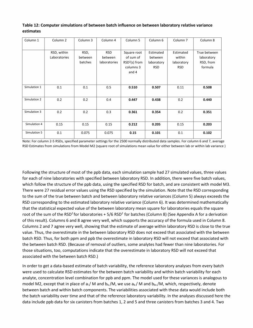
Table 12: Computer simulations of between batch influence on between laboratory relative variance estimates
Column 1 Column 2 Column 3 Column 4 Column 5 Column 6 Column 7 Column 8
RSD, within Laboratories
RSD, between batches
RSD between
laboratories
Square root of sum of
RSD2(s) from columns 3
and 4
Estimated between
laboratory RSD
Estimated within
laboratory RSD
True between laboratory RSD, from formula
Simulation 1 0.1 0.1 0.5 0.510 0.507 0.11 0.508
Simulation 2 0.2 0.2 0.4 0.447 0.438 0.2 0.440
Simulation 3 0.2 0.2 0.3 0.361 0.354 0.2 0.351
Simulation 4 0.15 0.15 0.15 0.212 0.205 0.15 0.203
Simulation 5 0.1 0.075 0.075 0.15 0.101 0.1 0.102
Note: For column 2-5 RSDs, specified parameter settings for the 2500 normally distributed data samples. For column 6 and 7, average RSD Estimates from simulations from Model M2 (square root of simulations mean value for either between lab or within lab variance )
Following the structure of most of the ppb data, each simulation sample had 27 simulated values, three values for each of nine laboratories with specified between laboratory RSD. In addition, there were five batch values, which follow the structure of the ppb data, using the specified RSD for batch, and are consistent with model M3. There were 27 residual error values using the RSD specified by the simulation. Note that the RSD corresponding to the sum of the true between batch and between laboratory relative variances (Column 5) always exceeds the RSD corresponding to the estimated laboratory relative variance (Column 6). It was determined mathematically that the statistical expected value of the between laboratory mean square for laboratories equals the square root of the sum of the RSD2 for laboratories + 5/6 RSD2 for batches (Column 8) (See Appendix A for a derivation of this result). Columns 6 and 8 agree very well, which supports the accuracy of the formula used in Column 8. Columns 2 and 7 agree very well, showing that the estimate of average within laboratory RSD is close to the true value. Thus, the overestimate in the between laboratory RSD does not exceed that associated with the between batch RSD. Thus, for both ppm and ppb the overestimate in laboratory RSD will not exceed that associated with the between batch RSD. (Because of removal of outliers, some analytes had fewer than nine laboratories. For those situations, too, computations indicate that the overestimate in laboratory RSD will not exceed that associated with the between batch RSD.)
In order to get a data-based estimate of batch variability, the reference laboratory analyses from every batch were used to calculate RSD estimates for the between batch variability and within batch variability for each analyte, concentration level combination for ppb and ppm. The model used for these variances is analogous to model M2, except that in place of al / M and bls /M, we use ab / M and bbs /M, which, respectively, denote between batch and within batch components. The variabilities associated with these data would include both the batch variability over time and that of the reference laboratory variability. In the analyses discussed here the data include ppb data for six canisters from batches 1, 2 and 5 and three canisters from batches 3 and 4. Two
measurements at 5 ppb for each of three analytes were removed because of Grubbs tests. PPM results are based on three canisters for each of seven batches, except that at the 0.8 ppm level, two canisters were removed based on Grubbs tests.
We are interested in determining how much the between laboratory RSD is inflated by the between batch variability. Recall that the RSD values are relative to the average of the batch theoretical values for the given analyte and concentration level. Thus, all RSDs for each analyte, concentration level combination are divided by this average theoretical value. Each RSD can be converted to a standard deviation by multiplying it by the theoretical average. This is correct for both the model M2 for the laboratory data and the model discussed in the previous paragraph for the reference laboratory data. In accordance with the results shown above for ppm and ppb, a modified result for the laboratory RSD_ILS was calculated as:
lab RSD_ILS (mod) = [(lab RSD_ ILS)2 – (batch RSD_Reflab)2)]0.5,
In terms of the Table 11 data, lab RSD_ILS squared value is (0.077/0.846)2 = 0.092 = 0.0081, where 0.846 is the average theoretical value for the analyte at the given concentration, and 0.077 is the estimated standard deviation from the ILS. From the reference laboratory analysis, the batch RSD Reflab value is 0.024 / 0.846 and (0.024/0.846)2 = 0.0282 = 0.00078. Thus, lab RSD_ILS (mod) = sq. rt((0.077/0.846)2 - (0.024/0.846)2) = sq. rt. ( 0.0081- 0.00078) = 0.086. The lab RSD_ ILS value was 0.09. Thus the modified value differs from the estimated RSD by 0.09-0.086 = 0.004, a small difference. This supports the idea that the between batch variability is small compared to the between laboratory variability. The estimate 0.086 represents the estimate of the between laboratory RSD, after removing the variability associated with the between batch variability. We know from the statistical analysis results above that, on average, the estimated between laboratory RSD2 from the ILS study will not exceed the true between laboratory RSD2 by more than the between batch RSD2 (here 0.00078); by removing this excess we can determine the effect of between batch variability on the between laboratory RSD estimates.
The aim of this work is not to replace the RSDs of the ILS by the modified values. We wish to see if the modified (“mod”) estimates support the reasonableness of the unmodified estimates. We will assess this by determining the size of the difference between the original estimates and the modified estimates. Note that there are models for which the RSDs from the reference laboratory data exceeded those from the ILS study, which led to negative differences of [(lab RSD_ ILS)2 – (batch RSD_Reflab)2)], for which a square root could not be taken to calculate lab RSD_ILS (mod). There were twelve negative differences for [(lab RSD_ ILS)2 – (batch RSD_Reflab)2)]. For all twelve differences, lab RSD_ ILS values were less than 0.1, and six were less than 0.01. This kind of result is not unexpected, where the variances are based on models with small sample size and when lab RSD_ ILS values are small. Set DIF=lab RSD_ILS -lab RSD_ILS (mod) when lab RSD_ILS (mod) can be calculated. Ideally DIF values are small, which indicates that when the variability associated with between batch variation is removed, the between laboratory estimates change little. There were four instances among the 102 models where DIF exceeded 0.05. The largest difference was 0.11. This result, together with the fact that the cases for which the reference laboratory between batch RSD estimate exceeded the ILS between laboratory RSD estimate occurred when the between laboratory ILS was less than 0.1, suggests that there seems little indication that between batch variability had large effect for many of the laboratory RSD estimates. Also we recognize that the between batch estimates from the reference laboratory data are overestimates, since the reference laboratory data include that lab’s variability, in addition to batch variability over time. Recall that the reference laboratory results from the first spike batches of ppm and ppb were used for the results in Tables 13 and 14. The above analysis indicates that estimated between laboratory RSDs from the inter-laboratory study would not vary much if another reference laboratory spike-batch were used, since the reference laboratory variability was usually much smaller than the between laboratory variability.
Bias across spike batches was also estimated using the reference laboratory data to ensure consistency in spike batch generation over time. Bias was fairly consistent, falling within ±10% of the theoretical value for most analytes and nominal levels for both ppb-range (Table B1, Appendix B) and ppm-range (Table B2, Appendix B). Representative box plots of bias are presented for ethanol (Figure 1 left) and for 2,3-butanedione (Figure 1 right). Excursions outside the ±10% criterion were observed for ethanol, which is notoriously difficult to analyze due to its low molecular weight and polarity, in spike 3 and 4 at 5, 10, and 15 ppb (Figure 1 top left). Additional excursions were observed for ppm-level range for ethanol (Figure 1 bottom left). Ethanol for spike batch 6 and 7 showed a positive bias compared to spike batches 1 to 5 due to the change in generation procedure. For 2,3- Butanedione, bias across spike batches was more stable with many boxes falling within the ±10% of the theoretical value.
Estimates of total RSD presented here are not significantly affected by these shifts in bias among different spike batch generations. Shifts in bias across batches are associated with between-batch variability, and as was stated above, the between-batch variability results in only small increases in the reproducibility RSD estimates for most analytes.
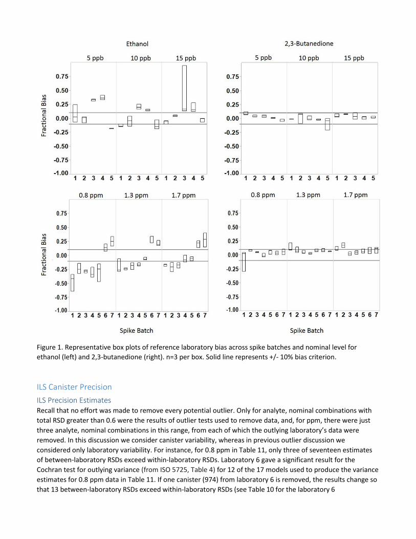
Figure 1. Representative box plots of reference laboratory bias across spike batches and nominal level for ethanol (left) and 2,3-butanedione (right). n=3 per box. Solid line represents +/- 10% bias criterion.
ILS Canister Precision ILS Precision Estimates Recall that no effort was made to remove every potential outlier. Only for analyte, nominal combinations with total RSD greater than 0.6 were the results of outlier tests used to remove data, and, for ppm, there were just three analyte, nominal combinations in this range, from each of which the outlying laboratory’s data were removed. In this discussion we consider canister variability, whereas in previous outlier discussion we considered only laboratory variability. For instance, for 0.8 ppm in Table 11, only three of seventeen estimates of between-laboratory RSDs exceed within-laboratory RSDs. Laboratory 6 gave a significant result for the Cochran test for outlying variance (from ISO 5725, Table 4) for 12 of the 17 models used to produce the variance estimates for 0.8 ppm data in Table 11. If one canister (974) from laboratory 6 is removed, the results change so that 13 between-laboratory RSDs exceed within-laboratory RSDs (see Table 10 for the laboratory 6
concentrations by canister and Table 11 for the Cochran test calculation). However, the reproducibility RSDs change by no more than 0.025. Note that canister 974 data were not omitted from the calculations shown in Table 11. The discussion above is included in order to show the sensitiveness of the results, not to remove any more data. We also note that there is no way to know whether between-batch variability is introduced during the generation process or by the participating laboratory during analysis.
The ppb-level results in Table 13 show mostly higher between- than within-laboratory RSDs (35/51 or 68.6%), and although the ppm do not, this may be partly due to the presence of some outliers. Also, the ratio of between to within laboratory RSD is quite high for ppb, on average about two.
When analysis of variance is computed separately for each level’s reproducibility values as function of analyte and concentration level, neither ppb nor ppm gives results significant at the 5% level.
There is useful information in the outlier analysis. Of the 75 values removed as outliers and not used in the estimates in Tables 13 and 14, all but six came from laboratories 5 and 7. Laboratory 7 produced 57 values, of which 42 were at 5 ppb, 12 were at 15 ppb, and three were at 0.8 ppm. Laboratory 5 produced 12, of which six were at ppb levels (three at 5 ppb and three at 15 ppb), and three at ppm levels. There were no outliers at the 10 ppb level or at the 1.7 ppm level. Thus, almost all outliers were for ppb levels. All outliers were for large magnitude measurements, that is, values larger than the mean. Thus, there is no surprise that the ppb estimates tended to have large between-laboratory RSDS than within-laboratory RSDs. In addition, ppb levels have more total variation than ppm. There are 10 reproducibility RSDs for ppb greater than or equal to 0.5 compared to three for ppm. Furthermore, there are 32 reproducibility RSDs for ppb greater than or equal to 0.3 compared to 11 for ppm. On the other hand, whereas the smallest reproducibility RSD for ppm is approximately 0.19, there are 14 ppb reproducibility RSDs less than or equal to 0.19. Thus, the ppm data have less spread in reproducibility than the ppb. Likewise, there are just two ppm within-laboratory RSDs less than or equal to 0.14 but 27 for ppb. There appear to be four ppm values less than or equal to 0.14 in Table 14, but that is just due to rounding. There are four ppb within-laboratory RSDs 0.3 or larger, compared to three for ppm. Thus, except for the high within- laboratory RSDs, ppb RSDs have a wider spread than ppm.
The reasons for these differences between ppb and ppm are not clear. It does seem that the low levels used for ppb are associated with large positive bias for some laboratories, although that does not occur at 10 ppb, where results look more like ppm level results than like ppb level results. Analytes are more alike at the ppm level than at the ppb level, in the sense that there are many ppb RSDs less than and others more than most ppm RSDs. This may mean that at high levels (ppm), the instructions for the method are followed better by all labs than at lower levels (ppb) or, perhaps more likely, method precision becomes poorer as analyte concentration decreases from ppm to ppb levels.
Also, RSDs for ppb may be influenced by some of the potential outlier laboratories, whose practices are discussed below (laboratories 5, 6, and 7).
In summary, for ppb, estimates for repeatability ranged from 0.04 to 0.55 and estimates for reproducibility ranged from 0.10 to 0.62. For ppm, estimates for repeatability ranged from 0.10 to 0.47 and for reproducibility from 0.19 to 0.58.
For comparison, ASTM D6196 provides some insight about precision estimates from thermal desorption tubes, a complementary sampling and detection technique that provides sensitive estimates of airborne VOC concentrations [14]. They reported mean ISO repeatability estimates between 0.072 and 0.216 for hydrocarbons C3 to C11 from Coker et al. [15] which are compared to canister method ILS results of within-laboratory RSDs from 0.04 to 0.55 with a median of 0.14 for ppb and from 0.1 to 0.47 with a median of 0.19 for ppm. They reported ISO reproducibility estimates between 0.259 to 0.432 compared to canister method ILS results of total

RSDs from 0.1 to 0.62 with a median of 0.37 for ppb and from 0.19 to 0.58 to with a median of 0.23 for ppm. While some of these values are higher than those reported in ASTM D6196, more laboratories were used in this study (nine vs. four).
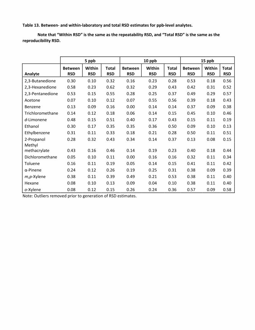
Table 13. Between- and within-laboratory and total RSD estimates for ppb-level analytes.
Note that “Within RSD” is the same as the repeatability RSD, and “Total RSD” is the same as the reproducibility RSD.
5 ppb 10 ppb 15 ppb
Analyte Between
RSD Within
RSD Total RSD
Between RSD
Within RSD
Total RSD
Between RSD
Within RSD
Total RSD
2,3-Butanedione 0.30 0.10 0.32 0.16 0.23 0.28 0.53 0.18 0.56 2,3-Hexanedione 0.58 0.23 0.62 0.32 0.29 0.43 0.42 0.31 0.52 2,3-Pentanedione 0.53 0.15 0.55 0.28 0.25 0.37 0.49 0.29 0.57 Acetone 0.07 0.10 0.12 0.07 0.55 0.56 0.39 0.18 0.43 Benzene 0.13 0.09 0.16 0.00 0.14 0.14 0.37 0.09 0.38 Trichloromethane 0.14 0.12 0.18 0.06 0.14 0.15 0.45 0.10 0.46 d-Limonene 0.48 0.15 0.51 0.40 0.17 0.43 0.15 0.11 0.19 Ethanol 0.30 0.17 0.35 0.35 0.36 0.50 0.09 0.10 0.13 Ethylbenzene 0.31 0.11 0.33 0.18 0.21 0.28 0.50 0.11 0.51 2-Propanol 0.28 0.32 0.43 0.34 0.14 0.37 0.13 0.08 0.15 Methyl methacrylate 0.43 0.16 0.46 0.14 0.19 0.23 0.40 0.18 0.44 Dichloromethane 0.05 0.10 0.11 0.00 0.16 0.16 0.32 0.11 0.34 Toluene 0.16 0.11 0.19 0.05 0.14 0.15 0.41 0.11 0.42 α-Pinene 0.24 0.12 0.26 0.19 0.25 0.31 0.38 0.09 0.39 m,p-Xylene 0.38 0.11 0.39 0.49 0.21 0.53 0.38 0.11 0.40 Hexane 0.08 0.10 0.13 0.09 0.04 0.10 0.38 0.11 0.40 o-Xylene 0.08 0.12 0.15 0.26 0.24 0.36 0.57 0.09 0.58
Note: Outliers removed prior to generation of RSD estimates.
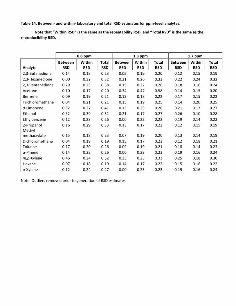
Table 14. Between- and within- laboratory and total RSD estimates for ppm-level analytes.
Note that “Within RSD” is the same as the repeatability RSD, and “Total RSD” is the same as the reproducibility RSD.
0.8 ppm 1.3 ppm 1.7 ppm
Analyte Between
RSD Within
RSD Total RSD
Between RSD
Within RSD
Total RSD
Between RSD
Within RSD
Total RSD
2,3-Butanedione 0.14 0.18 0.23 0.05 0.19 0.20 0.12 0.15 0.19 2,3-Hexanedione 0.00 0.32 0.32 0.21 0.26 0.33 0.22 0.24 0.32 2,3-Pentanedione 0.29 0.25 0.38 0.15 0.22 0.26 0.18 0.16 0.24 Acetone 0.10 0.17 0.20 0.34 0.47 0.58 0.14 0.15 0.20 Benzene 0.09 0.19 0.21 0.13 0.18 0.22 0.17 0.15 0.22 Trichloromethane 0.04 0.21 0.21 0.15 0.19 0.25 0.14 0.20 0.25 d-Limonene 0.32 0.27 0.41 0.13 0.23 0.26 0.21 0.17 0.27 Ethanol 0.32 0.39 0.51 0.21 0.17 0.27 0.26 0.10 0.28 Ethylbenzene 0.12 0.23 0.26 0.00 0.22 0.22 0.19 0.14 0.23 2-Propanol 0.16 0.29 0.33 0.13 0.17 0.22 0.12 0.15 0.19 Methylmethacrylate 0.15 0.18 0.23 0.07 0.19 0.20 0.13 0.14 0.19 Dichloromethane 0.04 0.19 0.19 0.15 0.17 0.23 0.12 0.18 0.21 Toluene 0.17 0.20 0.26 0.09 0.19 0.21 0.18 0.14 0.23 α-Pinene 0.14 0.22 0.26 0.00 0.23 0.23 0.19 0.16 0.24 m,p-Xylene 0.46 0.24 0.52 0.23 0.23 0.33 0.25 0.18 0.30 Hexane 0.07 0.18 0.19 0.14 0.17 0.22 0.15 0.16 0.22 o-Xylene 0.12 0.24 0.27 0.00 0.23 0.23 0.19 0.16 0.24
Note: Outliers removed prior to generation of RSD estimates.
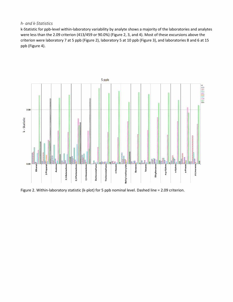
h- and k-Statisticsk-Statistic for ppb-level within-laboratory variability by analyte shows a majority of the laboratories and analyteswere less than the 2.09 criterion (413/459 or 90.0%) (Figure 2, 3, and 4). Most of these excursions above thecriterion were laboratory 7 at 5 ppb (Figure 2), laboratory 5 at 10 ppb (Figure 3), and laboratories 8 and 6 at 15ppb (Figure 4).
Figure 2. Within-laboratory statistic (k-plot) for 5 ppb nominal level. Dashed line = 2.09 criterion.
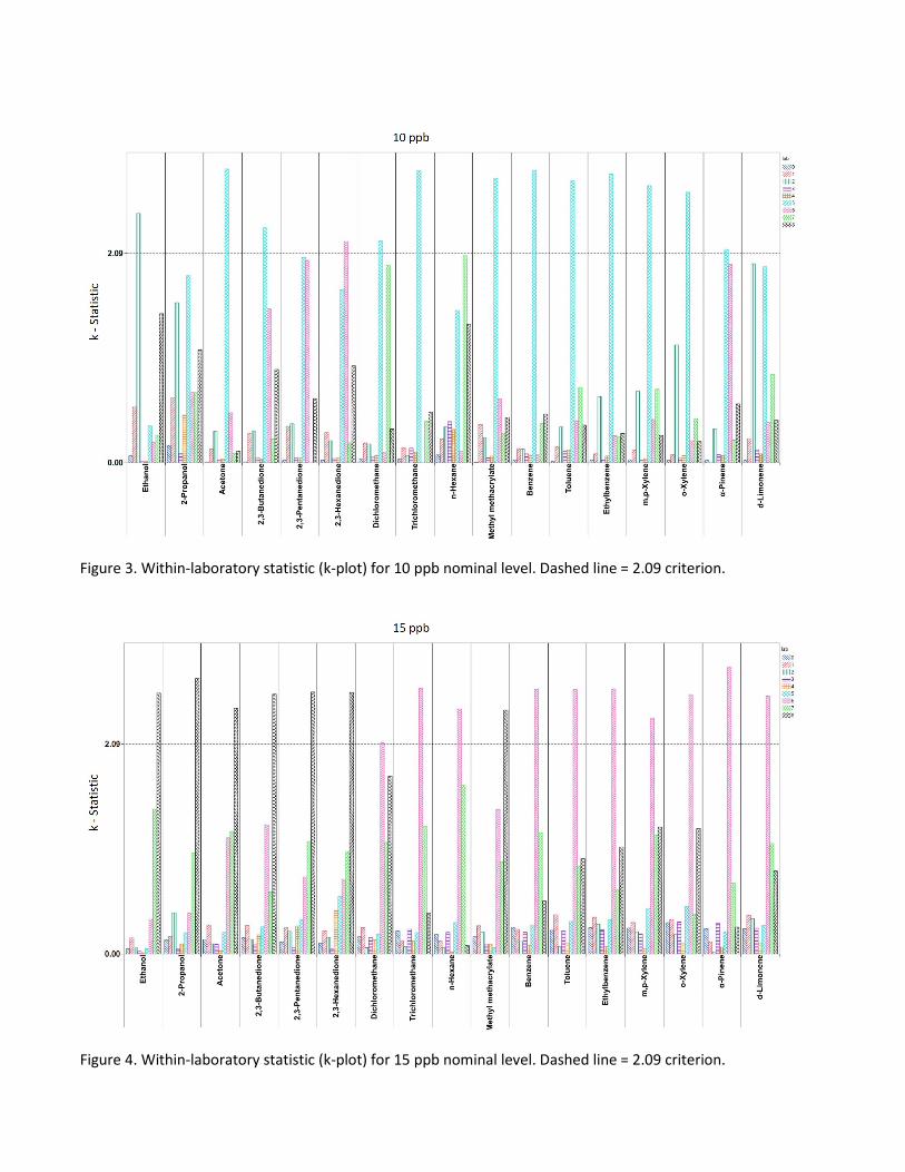
Figure 3. Within-laboratory statistic (k-plot) for 10 ppb nominal level. Dashed line = 2.09 criterion.
Figure 4. Within-laboratory statistic (k-plot) for 15 ppb nominal level. Dashed line = 2.09 criterion.
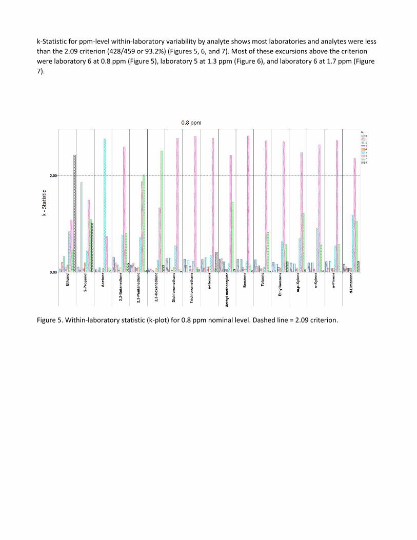
k-Statistic for ppm-level within-laboratory variability by analyte shows most laboratories and analytes were lessthan the 2.09 criterion (428/459 or 93.2%) (Figures 5, 6, and 7). Most of these excursions above the criterionwere laboratory 6 at 0.8 ppm (Figure 5), laboratory 5 at 1.3 ppm (Figure 6), and laboratory 6 at 1.7 ppm (Figure7).
Figure 5. Within-laboratory statistic (k-plot) for 0.8 ppm nominal level. Dashed line = 2.09 criterion.
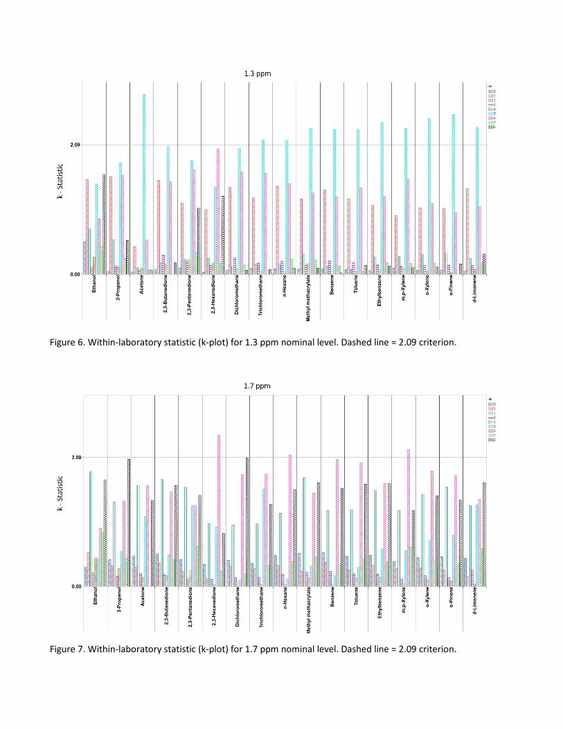
Figure 6. Within-laboratory statistic (k-plot) for 1.3 ppm nominal level. Dashed line = 2.09 criterion.
Figure 7. Within-laboratory statistic (k-plot) for 1.7 ppm nominal level. Dashed line = 2.09 criterion.
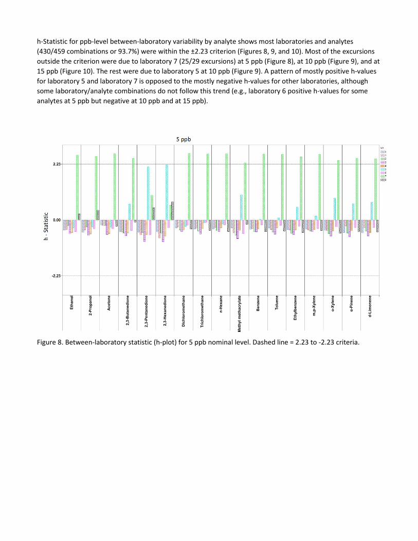
h-Statistic for ppb-level between-laboratory variability by analyte shows most laboratories and analytes(430/459 combinations or 93.7%) were within the ±2.23 criterion (Figures 8, 9, and 10). Most of the excursionsoutside the criterion were due to laboratory 7 (25/29 excursions) at 5 ppb (Figure 8), at 10 ppb (Figure 9), and at15 ppb (Figure 10). The rest were due to laboratory 5 at 10 ppb (Figure 9). A pattern of mostly positive h-valuesfor laboratory 5 and laboratory 7 is opposed to the mostly negative h-values for other laboratories, althoughsome laboratory/analyte combinations do not follow this trend (e.g., laboratory 6 positive h-values for someanalytes at 5 ppb but negative at 10 ppb and at 15 ppb).
Figure 8. Between-laboratory statistic (h-plot) for 5 ppb nominal level. Dashed line = 2.23 to -2.23 criteria.
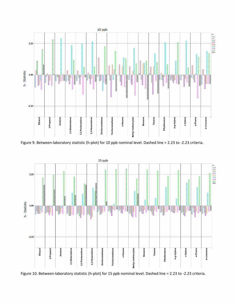
Figure 9. Between-laboratory statistic (h-plot) for 10 ppb nominal level. Dashed line = 2.23 to -2.23 criteria.
Figure 10. Between-laboratory statistic (h-plot) for 15 ppb nominal level. Dashed line = 2.23 to -2.23 criteria.
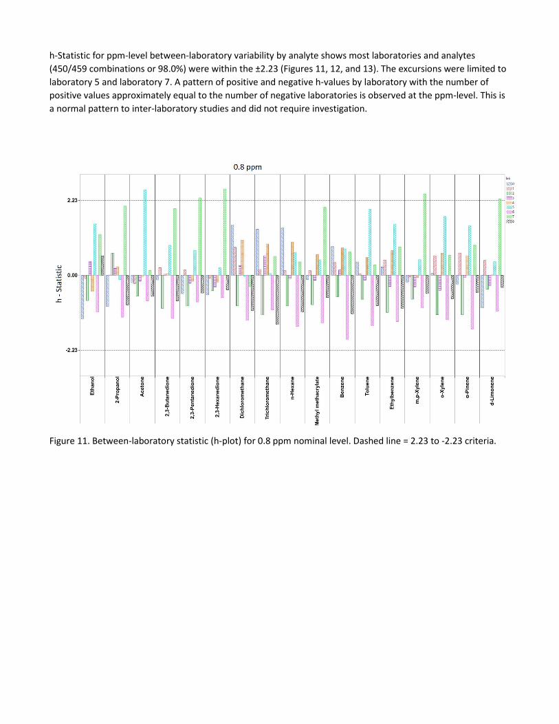
h-Statistic for ppm-level between-laboratory variability by analyte shows most laboratories and analytes(450/459 combinations or 98.0%) were within the ±2.23 (Figures 11, 12, and 13). The excursions were limited tolaboratory 5 and laboratory 7. A pattern of positive and negative h-values by laboratory with the number ofpositive values approximately equal to the number of negative laboratories is observed at the ppm-level. This isa normal pattern to inter-laboratory studies and did not require investigation.
Figure 11. Between-laboratory statistic (h-plot) for 0.8 ppm nominal level. Dashed line = 2.23 to -2.23 criteria.
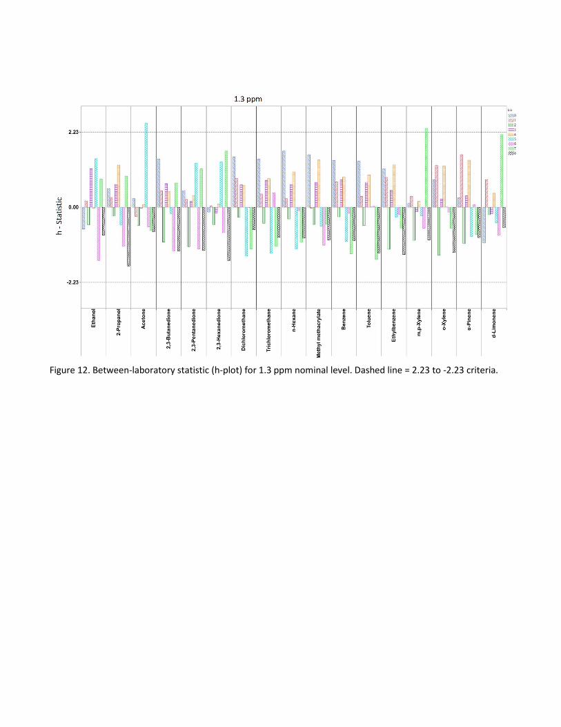
Figure 12. Between-laboratory statistic (h-plot) for 1.3 ppm nominal level. Dashed line = 2.23 to -2.23 criteria.
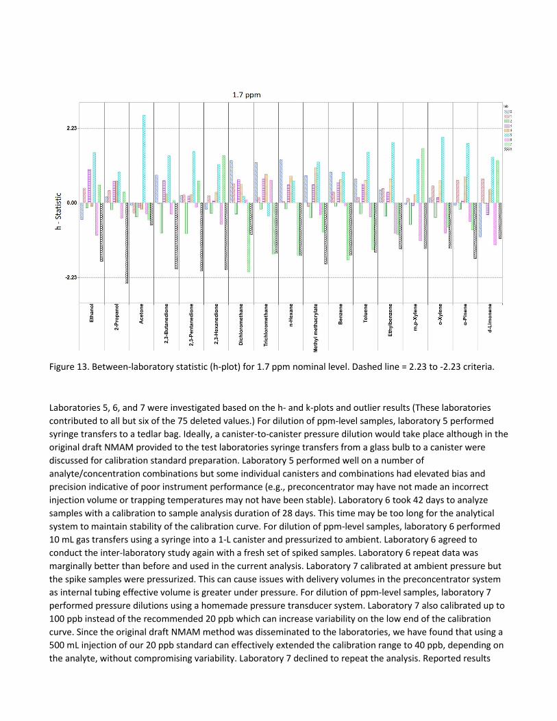
Figure 13. Between-laboratory statistic (h-plot) for 1.7 ppm nominal level. Dashed line = 2.23 to -2.23 criteria.
Laboratories 5, 6, and 7 were investigated based on the h- and k-plots and outlier results (These laboratories contributed to all but six of the 75 deleted values.) For dilution of ppm-level samples, laboratory 5 performed syringe transfers to a tedlar bag. Ideally, a canister-to-canister pressure dilution would take place although in the original draft NMAM provided to the test laboratories syringe transfers from a glass bulb to a canister were discussed for calibration standard preparation. Laboratory 5 performed well on a number of analyte/concentration combinations but some individual canisters and combinations had elevated bias and precision indicative of poor instrument performance (e.g., preconcentrator may have not made an incorrect injection volume or trapping temperatures may not have been stable). Laboratory 6 took 42 days to analyze samples with a calibration to sample analysis duration of 28 days. This time may be too long for the analytical system to maintain stability of the calibration curve. For dilution of ppm-level samples, laboratory 6 performed 10 mL gas transfers using a syringe into a 1-L canister and pressurized to ambient. Laboratory 6 agreed to conduct the inter-laboratory study again with a fresh set of spiked samples. Laboratory 6 repeat data was marginally better than before and used in the current analysis. Laboratory 7 calibrated at ambient pressure but the spike samples were pressurized. This can cause issues with delivery volumes in the preconcentrator system as internal tubing effective volume is greater under pressure. For dilution of ppm-level samples, laboratory 7 performed pressure dilutions using a homemade pressure transducer system. Laboratory 7 also calibrated up to 100 ppb instead of the recommended 20 ppb which can increase variability on the low end of the calibration curve. Since the original draft NMAM method was disseminated to the laboratories, we have found that using a 500 mL injection of our 20 ppb standard can effectively extended the calibration range to 40 ppb, depending on the analyte, without compromising variability. Laboratory 7 declined to repeat the analysis. Reported results
from Laboratory 7 were quite different from theoretical values indicating an incorrect calibration standard preparation at the laboratory or poorly prepared spikes, although reference canisters for this trial did not indicate poor preparation. Large variability in Laboratory 7 data may have been due to preconcentrator system instability and/or a higher than normal dynamic range of 5 to 100 ppb. In particular, 5 ppb results were much higher than other labs, and most of the analytes were identified as outliers at 5 ppb for laboratory 7.
ILS Conclusions Precision estimates for repeatability ranged from 0.04 to 0.55 at ppb concentrations and from 0.10 to 0.47 for ppm concentrations. Precision estimates for reproducibility ranged from 0.10 to 0.62 at ppb concentrations and from 0.19 to 0.58 at ppm concentrations, depending on analyte and nominal. Plots of h- and k-statistics indicated inconsistencies with reported results from laboratories 5, 6, and 7. These laboratories were investigated to determine the cause of the inconsistent results. Issues with storage time and adherence to the method protocol were encountered but results were retained due to the low number of laboratories participating. Precision varied by laboratory with more than half of the laboratories performing well indicating a fairly robust method across laboratories. Training on pressure dilution techniques and preconcentration systems as well as proficiency testing should be periodically conducted to ensure operating laboratories maintain optimal canister method performance.
References 1. Code of Federal Regulations [2017]. Title 29 (Labor), Part 1910 (Occupational Safety and Health
Standards); 29 CFR 1910.1000 Table Z-1; US Government Printing Office, Washington DC. 2. NIOSH [2010]. Pocket Guide to Chemical Hazards. Cincinnati, OH: U.S. Department of Health and Human
Services, Centers for Disease Control and Prevention, National Institute for Occupational Safety and Health, DHHS (NIOSH) Publication No. 2010-168c. Available from: http://www.cdc.gov/niosh/npg/default.html.
3. EPA [1999]. Compendium Method TO-14A: Determination of volatile organic compounds (VOCs) in ambient air using specially prepared canisters with subsequent analysis by gas chromatography. Cincinnati, OH, U.S. Environmental Protection Agency, EPA/625/R-96/010b.
4. LeBouf RF, Stefaniak AB, Virji MA [2012]. Validation of evacuated canisters for sampling volatile organic compounds in healthcare settings. J Environ Monit 14(3):977-983.
5. Jia C, Batterman S, Chernyak S [2006]. Development and comparison of methods using MS scan and selective ion monitoring modes for a wide range of airborne VOCs. J Environ Monit. 8(10):1029-1042.
6. NIOSH [1995]. Guidelines for air sampling and analytical method development and evaluation. By Kennedy ER, Fischbach TJ, Song R, Eller PM, Shulman SA. Cincinnati, OH: U.S. Department of Health and Human Services, Centers for Disease Control and Prevention, National Institute for Occupational Safety and Health, DHHS (NIOSH) Publication No. 95-117.
7. Forester C, Wells J [2009]. Yields of Carbonyl Products from Gas-Phase Reactions of Fragrance Compounds with OH Radical and Ozone. Environ Sci Technol 43(10):3561-3568.
8. Atkinson R, Arey J [2003] Gas-phase tropospheric chemistry of biogenic volatile organic compounds: a review. Atmos Environ 37:S197-S219.
9. ASTM [2013]. D6246: Standard practice for evaluating the performance of diffusive samplers. ASTM International: West Conshohocken, PA.
10. LeBouf RF, Simmons M [2017]. Increased sensitivity of OSHA method analysis of diacetyl and 2,3- pentanedione in air. J Occup Environ Hyg 14(5):343-348.
11. Bartley DL [2001]. Definition and assessment of sampling and analytical accuracy. Annals Occup Hyg 45(5):357-364.
12. ASTM [2012]. Standard practice for conducting an interlaboratory study to determine the precision of a test method, in E691. ASTM International: West Conshohocken, PA.
13. ISO [1994]. 5725-2: Accuracy (trueness and precision) of measurement methods and results. 14. ASTM [2009]. D6193: Standard practice for selection of sorbents, sampling, and thermal desorption
analysis procedures for volatile organic compounds in air. ASTM International: West Conshohocken, PA. 15. Coker D, van den Hoed N, Saunders KJ, Tindle PE [1989]. A monitoring method for gasoline vapour giving
detailed composition. Ann Occup Hyg 33(1):15-26. 16. Scheffé H [1959]. The analysis of variance. New York: Wiley. 17. Parzen E [1960]. Modern probability theory and its application. New York: Wiley.

Appendix A: Backup Data for Spiking Experiments, LOD, and Stability
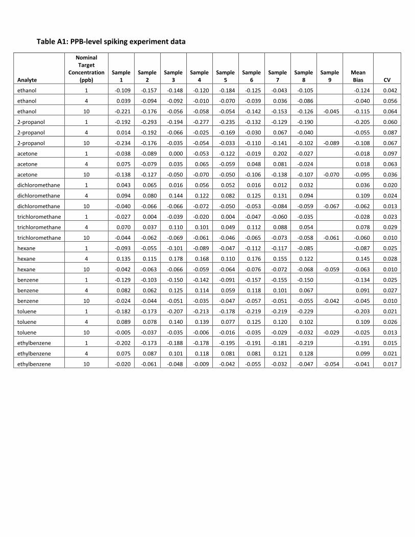
Table A1: PPB-level spiking experiment data
Analyte
Nominal Target
Concentration (ppb)
Sample 1
Sample 2
Sample 3
Sample 4
Sample 5
Sample 6
Sample 7
Sample 8
Sample 9
Mean Bias
CV
ethanol 1 -0.109 -0.157 -0.148 -0.120 -0.184 -0.125 -0.043 -0.105 -0.124 0.042
ethanol 4 0.039 -0.094 -0.092 -0.010 -0.070 -0.039 0.036 -0.086 -0.040 0.056
ethanol 10 -0.221 -0.176 -0.056 -0.058 -0.054 -0.142 -0.153 -0.126 -0.045 -0.115 0.064
2-propanol 1 -0.192 -0.293 -0.194 -0.277 -0.235 -0.132 -0.129 -0.190 -0.205 0.060
2-propanol 4 0.014 -0.192 -0.066 -0.025 -0.169 -0.030 0.067 -0.040 -0.055 0.087
2-propanol 10 -0.234 -0.176 -0.035 -0.054 -0.033 -0.110 -0.141 -0.102 -0.089 -0.108 0.067
acetone 1 -0.038 -0.089 0.000 -0.053 -0.122 -0.019 0.202 -0.027 -0.018 0.097
acetone 4 0.075 -0.079 0.035 0.065 -0.059 0.048 0.081 -0.024 0.018 0.063
acetone 10 -0.138 -0.127 -0.050 -0.070 -0.050 -0.106 -0.138 -0.107 -0.070 -0.095 0.036
dichloromethane 1 0.043 0.065 0.016 0.056 0.052 0.016 0.012 0.032 0.036 0.020
dichloromethane 4 0.094 0.080 0.144 0.122 0.082 0.125 0.131 0.094 0.109 0.024
dichloromethane 10 -0.040 -0.066 -0.066 -0.072 -0.050 -0.053 -0.084 -0.059 -0.067 -0.062 0.013
trichloromethane 1 -0.027 0.004 -0.039 -0.020 0.004 -0.047 -0.060 -0.035 -0.028 0.023
trichloromethane 4 0.070 0.037 0.110 0.101 0.049 0.112 0.088 0.054 0.078 0.029
trichloromethane 10 -0.044 -0.062 -0.069 -0.061 -0.046 -0.065 -0.073 -0.058 -0.061 -0.060 0.010
hexane 1 -0.093 -0.055 -0.101 -0.089 -0.047 -0.112 -0.117 -0.085 -0.087 0.025
hexane 4 0.135 0.115 0.178 0.168 0.110 0.176 0.155 0.122 0.145 0.028
hexane 10 -0.042 -0.063 -0.066 -0.059 -0.064 -0.076 -0.072 -0.068 -0.059 -0.063 0.010
benzene 1 -0.129 -0.103 -0.150 -0.142 -0.091 -0.157 -0.155 -0.150 -0.134 0.025
benzene 4 0.082 0.062 0.125 0.114 0.059 0.118 0.101 0.067 0.091 0.027
benzene 10 -0.024 -0.044 -0.051 -0.035 -0.047 -0.057 -0.051 -0.055 -0.042 -0.045 0.010
toluene 1 -0.182 -0.173 -0.207 -0.213 -0.178 -0.219 -0.219 -0.229 -0.203 0.021
toluene 4 0.089 0.078 0.140 0.139 0.077 0.125 0.120 0.102 0.109 0.026
toluene 10 -0.005 -0.037 -0.035 -0.006 -0.016 -0.035 -0.029 -0.032 -0.029 -0.025 0.013
ethylbenzene 1 -0.202 -0.173 -0.188 -0.178 -0.195 -0.191 -0.181 -0.219 -0.191 0.015
ethylbenzene 4 0.075 0.087 0.101 0.118 0.081 0.081 0.121 0.128 0.099 0.021
ethylbenzene 10 -0.020 -0.061 -0.048 -0.009 -0.042 -0.055 -0.032 -0.047 -0.054 -0.041 0.017
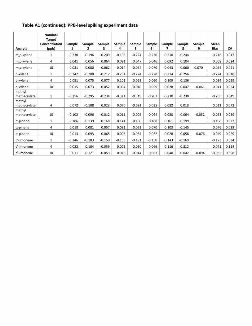
Table A1 (continued): PPB-level spiking experiment data
Analyte
Nominal Target
Concentration (ppb)
Sample 1
Sample 2
Sample 3
Sample 4
Sample 5
Sample 6
Sample 7
Sample 8
Sample 9
Mean Bias
CV
m,p-xylene 1 -0.230 -0.196 -0.209 -0.193 -0.224 -0.220 -0.210 -0.244 -0.216 0.017
m,p-xylene 4 0.041 0.056 0.064 0.091 0.047 0.046 0.092 0.104 0.068 0.024
m,p-xylene 10 -0.031 -0.080 -0.062 -0.014 -0.054 -0.070 -0.043 -0.060 -0.070 -0.054 0.021
o-xylene 1 -0.242 -0.208 -0.217 -0.201 -0.224 -0.228 -0.214 -0.256 -0.224 0.018
o-xylene 4 0.051 0.075 0.077 0.101 0.062 0.060 0.109 0.136 0.084 0.029
o-xylene 10 -0.015 -0.073 -0.052 0.004 -0.040 -0.059 -0.028 -0.047 -0.061 -0.041 0.024 methyl methacrylate
1
-0.256
-0.295
-0.234
-0.314
-0.349
-0.207
-0.230
-0.230
-0.265
0.049
methyl methacrylate
4
0.072
-0.108
0.023
0.070
-0.092
0.035
0.082
0.013
0.012
0.073
methyl methacrylate
10
-0.102
-0.096
-0.012
-0.011
0.005
-0.064
-0.080
-0.064
-0.052
-0.053
0.039
α-pinene 1 -0.186 -0.139 -0.168 -0.141 -0.160 -0.188 -0.161 -0.199 -0.168 0.022
α-pinene 4 0.018 0.081 0.057 0.081 0.052 0.070 0.103 0.145 0.076 0.038
α-pinene 10 -0.013 -0.093 -0.065 -0.006 -0.054 -0.052 -0.028 -0.058 -0.076 -0.049 0.029
d-limonene 1 -0.246 -0.183 -0.150 -0.156 -0.191 -0.150 -0.143 -0.169 -0.173 0.034
d-limonene 4 -0.022 0.104 -0.059 0.021 0.030 0.066 0.116 0.312 0.071 0.114
d-limonene 10 0.011 -0.121 -0.053 0.048 -0.044 -0.063 0.040 -0.042 -0.094 -0.035 0.058
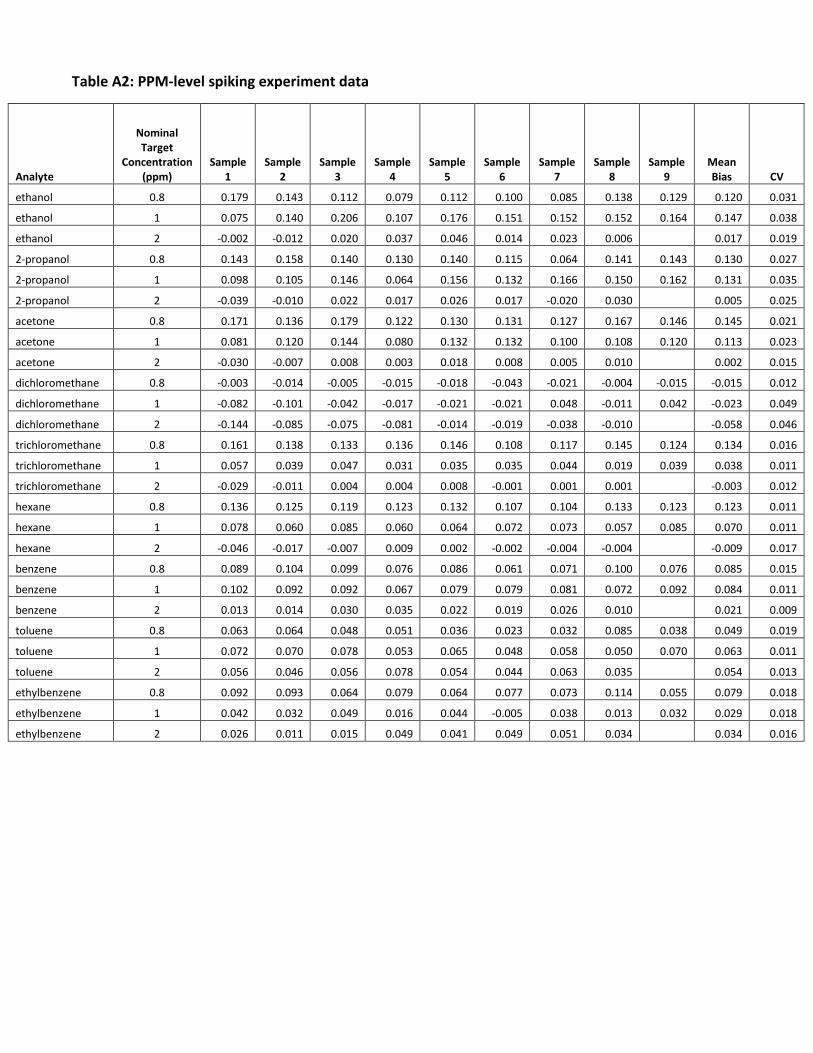
Table A2: PPM-level spiking experiment data
Analyte
Nominal Target
Concentration (ppm)
Sample
1
Sample
2
Sample
3
Sample
4
Sample
5
Sample
6
Sample
7
Sample
8
Sample
9
Mean Bias
CV
ethanol 0.8 0.179 0.143 0.112 0.079 0.112 0.100 0.085 0.138 0.129 0.120 0.031
ethanol 1 0.075 0.140 0.206 0.107 0.176 0.151 0.152 0.152 0.164 0.147 0.038
ethanol 2 -0.002 -0.012 0.020 0.037 0.046 0.014 0.023 0.006 0.017 0.019
2-propanol 0.8 0.143 0.158 0.140 0.130 0.140 0.115 0.064 0.141 0.143 0.130 0.027
2-propanol 1 0.098 0.105 0.146 0.064 0.156 0.132 0.166 0.150 0.162 0.131 0.035
2-propanol 2 -0.039 -0.010 0.022 0.017 0.026 0.017 -0.020 0.030 0.005 0.025
acetone 0.8 0.171 0.136 0.179 0.122 0.130 0.131 0.127 0.167 0.146 0.145 0.021
acetone 1 0.081 0.120 0.144 0.080 0.132 0.132 0.100 0.108 0.120 0.113 0.023
acetone 2 -0.030 -0.007 0.008 0.003 0.018 0.008 0.005 0.010 0.002 0.015
dichloromethane 0.8 -0.003 -0.014 -0.005 -0.015 -0.018 -0.043 -0.021 -0.004 -0.015 -0.015 0.012
dichloromethane 1 -0.082 -0.101 -0.042 -0.017 -0.021 -0.021 0.048 -0.011 0.042 -0.023 0.049
dichloromethane 2 -0.144 -0.085 -0.075 -0.081 -0.014 -0.019 -0.038 -0.010 -0.058 0.046
trichloromethane 0.8 0.161 0.138 0.133 0.136 0.146 0.108 0.117 0.145 0.124 0.134 0.016
trichloromethane 1 0.057 0.039 0.047 0.031 0.035 0.035 0.044 0.019 0.039 0.038 0.011
trichloromethane 2 -0.029 -0.011 0.004 0.004 0.008 -0.001 0.001 0.001 -0.003 0.012
hexane 0.8 0.136 0.125 0.119 0.123 0.132 0.107 0.104 0.133 0.123 0.123 0.011
hexane 1 0.078 0.060 0.085 0.060 0.064 0.072 0.073 0.057 0.085 0.070 0.011
hexane 2 -0.046 -0.017 -0.007 0.009 0.002 -0.002 -0.004 -0.004 -0.009 0.017
benzene 0.8 0.089 0.104 0.099 0.076 0.086 0.061 0.071 0.100 0.076 0.085 0.015
benzene 1 0.102 0.092 0.092 0.067 0.079 0.079 0.081 0.072 0.092 0.084 0.011
benzene 2 0.013 0.014 0.030 0.035 0.022 0.019 0.026 0.010 0.021 0.009
toluene 0.8 0.063 0.064 0.048 0.051 0.036 0.023 0.032 0.085 0.038 0.049 0.019
toluene 1 0.072 0.070 0.078 0.053 0.065 0.048 0.058 0.050 0.070 0.063 0.011
toluene 2 0.056 0.046 0.056 0.078 0.054 0.044 0.063 0.035 0.054 0.013
ethylbenzene 0.8 0.092 0.093 0.064 0.079 0.064 0.077 0.073 0.114 0.055 0.079 0.018
ethylbenzene 1 0.042 0.032 0.049 0.016 0.044 -0.005 0.038 0.013 0.032 0.029 0.018
ethylbenzene 2 0.026 0.011 0.015 0.049 0.041 0.049 0.051 0.034 0.034 0.016
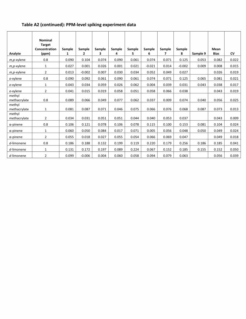
Table A2 (continued): PPM-level spiking experiment data
Analyte
Nominal Target
Concentration (ppm)
Sample
1
Sample
2
Sample
3
Sample
4
Sample
5
Sample
6
Sample
7
Sample
8
Sample 9
Mean Bias
CV
m,p-xylene 0.8 0.090 0.104 0.074 0.090 0.061 0.074 0.071 0.125 0.053 0.082 0.022
m,p-xylene 1 0.027 0.001 0.026 0.001 0.021 -0.021 0.014 -0.002 0.009 0.008 0.015
m,p-xylene 2 0.013 -0.002 0.007 0.030 0.034 0.052 0.049 0.027 0.026 0.019
o-xylene 0.8 0.090 0.092 0.061 0.090 0.061 0.074 0.071 0.125 0.065 0.081 0.021
o-xylene 1 0.043 0.034 0.059 0.026 0.062 0.004 0.039 0.031 0.043 0.038 0.017
o-xylene 2 0.041 0.015 0.019 0.058 0.051 0.058 0.066 0.038 0.043 0.019 methyl methacrylate
0.8
0.089
0.066
0.049
0.077
0.062
0.037
0.009
0.074
0.040
0.056
0.025
methyl methacrylate
1
0.081
0.087
0.071
0.046
0.075
0.066
0.076
0.068
0.087
0.073
0.013
methyl methacrylate
2
0.034
0.031
0.051
0.051
0.044
0.040
0.053
0.037
0.043
0.009
α-pinene 0.8 0.106 0.121 0.078 0.106 0.078 0.115 0.100 0.153 0.081 0.104 0.024
α-pinene 1 0.060 0.050 0.084 0.017 0.071 0.005 0.056 0.048 0.050 0.049 0.024
α-pinene 2 0.055 0.018 0.027 0.055 0.054 0.066 0.069 0.047 0.049 0.018
d-limonene 0.8 0.186 0.188 0.132 0.199 0.119 0.220 0.179 0.256 0.186 0.185 0.041
d-limonene 1 0.131 0.172 0.197 0.089 0.224 0.067 0.152 0.185 0.155 0.152 0.050
d-limonene 2 0.099 -0.006 0.004 0.060 0.058 0.094 0.079 0.063 0.056 0.039
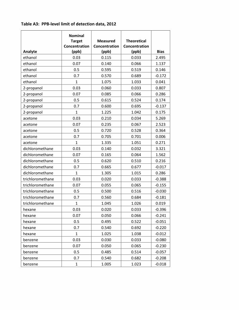
Table A3: PPB-level limit of detection data, 2012
Analyte
Nominal Target
Concentration (ppb)
Measured
Concentration (ppb)
Theoretical
Concentration (ppb)
Bias
ethanol 0.03 0.115 0.033 2.495 ethanol 0.07 0.140 0.066 1.137 ethanol 0.5 0.595 0.519 0.146 ethanol 0.7 0.570 0.689 -0.172 ethanol 1 1.075 1.033 0.041 2-propanol 0.03 0.060 0.033 0.807 2-propanol 0.07 0.085 0.066 0.286 2-propanol 0.5 0.615 0.524 0.174 2-propanol 0.7 0.600 0.695 -0.137 2-propanol 1 1.225 1.042 0.175 acetone 0.03 0.210 0.034 5.269 acetone 0.07 0.235 0.067 2.523 acetone 0.5 0.720 0.528 0.364 acetone 0.7 0.705 0.701 0.006 acetone 1 1.335 1.051 0.271 dichloromethane 0.03 0.140 0.032 3.321 dichloromethane 0.07 0.165 0.064 1.562 dichloromethane 0.5 0.620 0.510 0.216 dichloromethane 0.7 0.665 0.677 -0.017 dichloromethane 1 1.305 1.015 0.286 trichloromethane 0.03 0.020 0.033 -0.388 trichloromethane 0.07 0.055 0.065 -0.155 trichloromethane 0.5 0.500 0.516 -0.030 trichloromethane 0.7 0.560 0.684 -0.181 trichloromethane 1 1.045 1.026 0.019 hexane 0.03 0.020 0.033 -0.396 hexane 0.07 0.050 0.066 -0.241 hexane 0.5 0.495 0.522 -0.051 hexane 0.7 0.540 0.692 -0.220 hexane 1 1.025 1.038 -0.012 benzene 0.03 0.030 0.033 -0.080 benzene 0.07 0.050 0.065 -0.230 benzene 0.5 0.485 0.514 -0.057 benzene 0.7 0.540 0.682 -0.208 benzene 1 1.005 1.023 -0.018
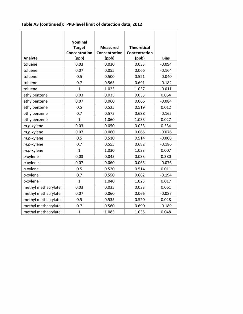
Table A3 (continued): PPB-level limit of detection data, 2012
Analyte
Nominal Target
Concentration (ppb)
Measured Concentration
(ppb)
Theoretical Concentration
(ppb)
Bias toluene 0.03 0.030 0.033 -0.094 toluene 0.07 0.055 0.066 -0.164 toluene 0.5 0.500 0.521 -0.040 toluene 0.7 0.565 0.691 -0.182 toluene 1 1.025 1.037 -0.011 ethylbenzene 0.03 0.035 0.033 0.064 ethylbenzene 0.07 0.060 0.066 -0.084 ethylbenzene 0.5 0.525 0.519 0.012 ethylbenzene 0.7 0.575 0.688 -0.165 ethylbenzene 1 1.060 1.033 0.027 m,p-xylene 0.03 0.050 0.033 0.534 m,p-xylene 0.07 0.060 0.065 -0.076 m,p-xylene 0.5 0.510 0.514 -0.008 m,p-xylene 0.7 0.555 0.682 -0.186 m,p-xylene 1 1.030 1.023 0.007 o-xylene 0.03 0.045 0.033 0.380 o-xylene 0.07 0.060 0.065 -0.076 o-xylene 0.5 0.520 0.514 0.011 o-xylene 0.7 0.550 0.682 -0.194 o-xylene 1 1.040 1.023 0.017 methyl methacrylate 0.03 0.035 0.033 0.061 methyl methacrylate 0.07 0.060 0.066 -0.087 methyl methacrylate 0.5 0.535 0.520 0.028 methyl methacrylate 0.7 0.560 0.690 -0.189 methyl methacrylate 1 1.085 1.035 0.048
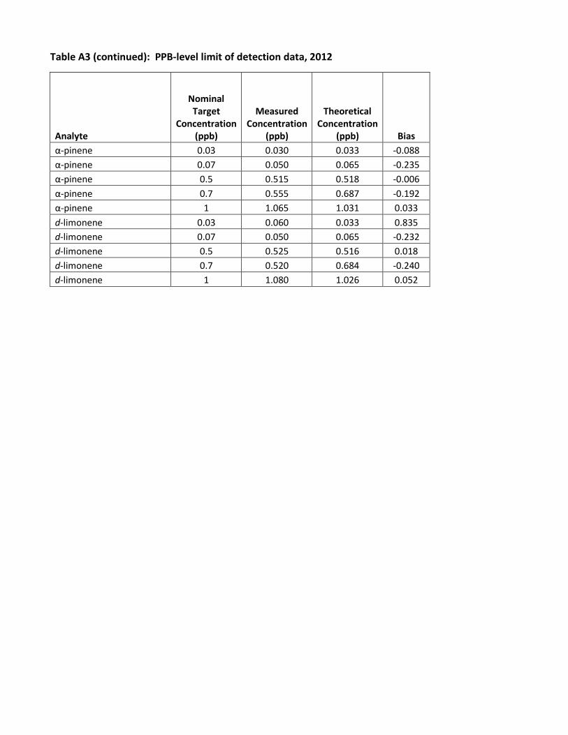
Table A3 (continued): PPB-level limit of detection data, 2012
Analyte
Nominal Target
Concentration (ppb)
Measured Concentration
(ppb)
Theoretical Concentration
(ppb) Bias α-pinene 0.03 0.030 0.033 -0.088α-pinene 0.07 0.050 0.065 -0.235α-pinene 0.5 0.515 0.518 -0.006α-pinene 0.7 0.555 0.687 -0.192α-pinene 1 1.065 1.031 0.033 d-limonene 0.03 0.060 0.033 0.835 d-limonene 0.07 0.050 0.065 -0.232d-limonene 0.5 0.525 0.516 0.018 d-limonene 0.7 0.520 0.684 -0.240d-limonene 1 1.080 1.026 0.052
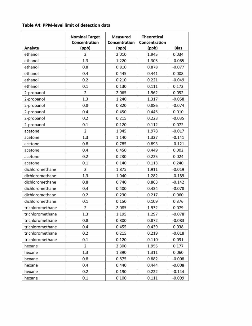
Table A4: PPM-level limit of detection data
Analyte
Nominal Target Concentration
(ppb)
Measured Concentration
(ppb)
Theoretical Concentration
(ppb) Bias ethanol 2 2.010 1.945 0.034 ethanol 1.3 1.220 1.305 -0.065ethanol 0.8 0.810 0.878 -0.077ethanol 0.4 0.445 0.441 0.008 ethanol 0.2 0.210 0.221 -0.049ethanol 0.1 0.130 0.111 0.172 2-propanol 2 2.065 1.962 0.052 2-propanol 1.3 1.240 1.317 -0.0582-propanol 0.8 0.820 0.886 -0.0742-propanol 0.4 0.450 0.445 0.010 2-propanol 0.2 0.215 0.223 -0.0352-propanol 0.1 0.120 0.112 0.072 acetone 2 1.945 1.978 -0.017acetone 1.3 1.140 1.327 -0.141acetone 0.8 0.785 0.893 -0.121acetone 0.4 0.450 0.449 0.002 acetone 0.2 0.230 0.225 0.024 acetone 0.1 0.140 0.113 0.240 dichloromethane 2 1.875 1.911 -0.019dichloromethane 1.3 1.040 1.282 -0.189dichloromethane 0.8 0.740 0.863 -0.142dichloromethane 0.4 0.400 0.434 -0.078dichloromethane 0.2 0.230 0.217 0.060 dichloromethane 0.1 0.150 0.109 0.376 trichloromethane 2 2.085 1.932 0.079 trichloromethane 1.3 1.195 1.297 -0.078trichloromethane 0.8 0.800 0.872 -0.083trichloromethane 0.4 0.455 0.439 0.038 trichloromethane 0.2 0.215 0.219 -0.018trichloromethane 0.1 0.120 0.110 0.091 hexane 2 2.300 1.955 0.177 hexane 1.3 1.390 1.311 0.060 hexane 0.8 0.875 0.882 -0.008hexane 0.4 0.440 0.444 -0.008hexane 0.2 0.190 0.222 -0.144hexane 0.1 0.100 0.111 -0.099
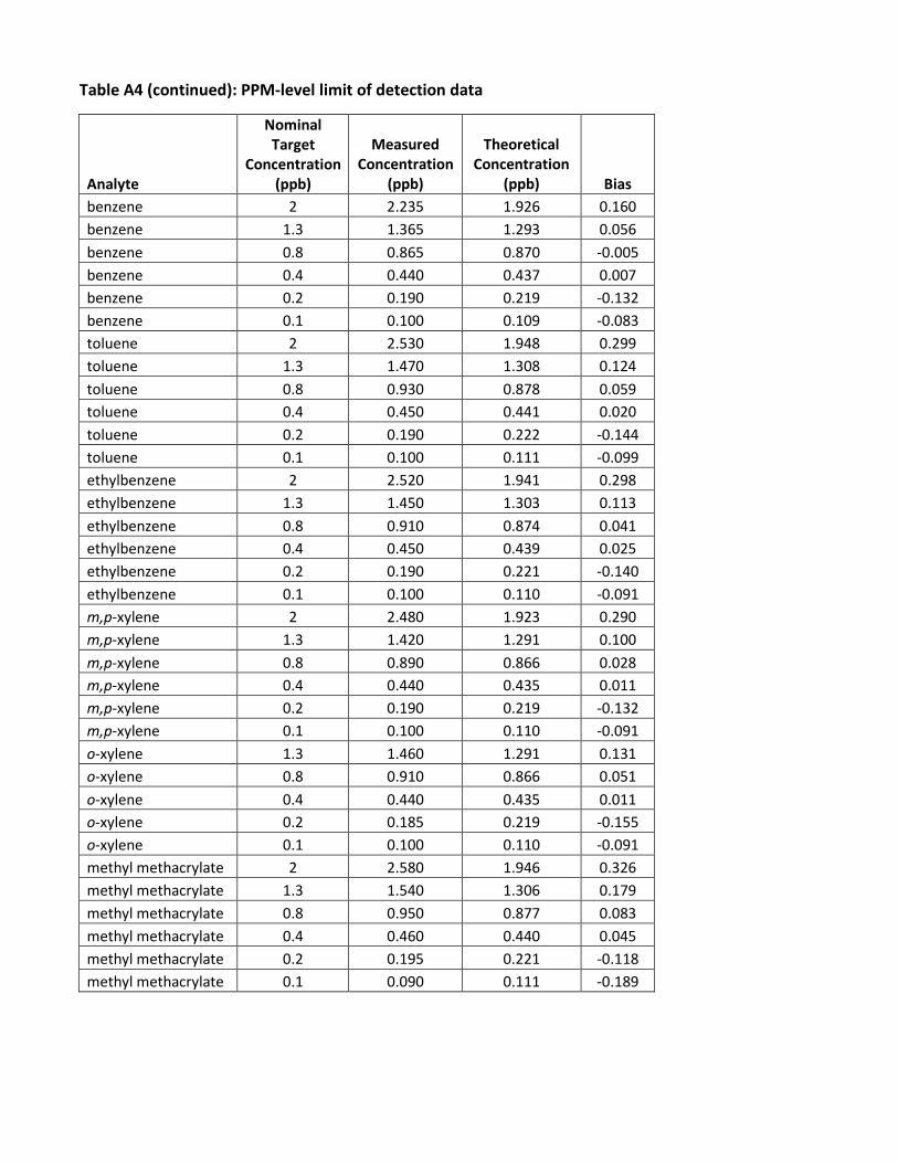
Table A4 (continued): PPM-level limit of detection data
Analyte
Nominal Target
Concentration (ppb)
Measured
Concentration (ppb)
Theoretical
Concentration (ppb)
Bias benzene 2 2.235 1.926 0.160 benzene 1.3 1.365 1.293 0.056 benzene 0.8 0.865 0.870 -0.005 benzene 0.4 0.440 0.437 0.007 benzene 0.2 0.190 0.219 -0.132 benzene 0.1 0.100 0.109 -0.083 toluene 2 2.530 1.948 0.299 toluene 1.3 1.470 1.308 0.124 toluene 0.8 0.930 0.878 0.059 toluene 0.4 0.450 0.441 0.020 toluene 0.2 0.190 0.222 -0.144 toluene 0.1 0.100 0.111 -0.099 ethylbenzene 2 2.520 1.941 0.298 ethylbenzene 1.3 1.450 1.303 0.113 ethylbenzene 0.8 0.910 0.874 0.041 ethylbenzene 0.4 0.450 0.439 0.025 ethylbenzene 0.2 0.190 0.221 -0.140 ethylbenzene 0.1 0.100 0.110 -0.091 m,p-xylene 2 2.480 1.923 0.290 m,p-xylene 1.3 1.420 1.291 0.100 m,p-xylene 0.8 0.890 0.866 0.028 m,p-xylene 0.4 0.440 0.435 0.011 m,p-xylene 0.2 0.190 0.219 -0.132 m,p-xylene 0.1 0.100 0.110 -0.091 o-xylene 1.3 1.460 1.291 0.131 o-xylene 0.8 0.910 0.866 0.051 o-xylene 0.4 0.440 0.435 0.011 o-xylene 0.2 0.185 0.219 -0.155 o-xylene 0.1 0.100 0.110 -0.091 methyl methacrylate 2 2.580 1.946 0.326 methyl methacrylate 1.3 1.540 1.306 0.179 methyl methacrylate 0.8 0.950 0.877 0.083 methyl methacrylate 0.4 0.460 0.440 0.045 methyl methacrylate 0.2 0.195 0.221 -0.118 methyl methacrylate 0.1 0.090 0.111 -0.189
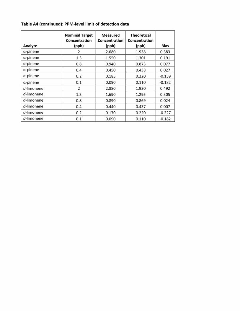
Table A4 (continued): PPM-level limit of detection data
Analyte
Nominal Target Concentration
(ppb)
Measured Concentration
(ppb)
Theoretical Concentration
(ppb)
Bias α-pinene 2 2.680 1.938 0.383 α-pinene 1.3 1.550 1.301 0.191 α-pinene 0.8 0.940 0.873 0.077 α-pinene 0.4 0.450 0.438 0.027 α-pinene 0.2 0.185 0.220 -0.159 α-pinene 0.1 0.090 0.110 -0.182 d-limonene 2 2.880 1.930 0.492 d-limonene 1.3 1.690 1.295 0.305 d-limonene 0.8 0.890 0.869 0.024 d-limonene 0.4 0.440 0.437 0.007 d-limonene 0.2 0.170 0.220 -0.227 d-limonene 0.1 0.090 0.110 -0.182
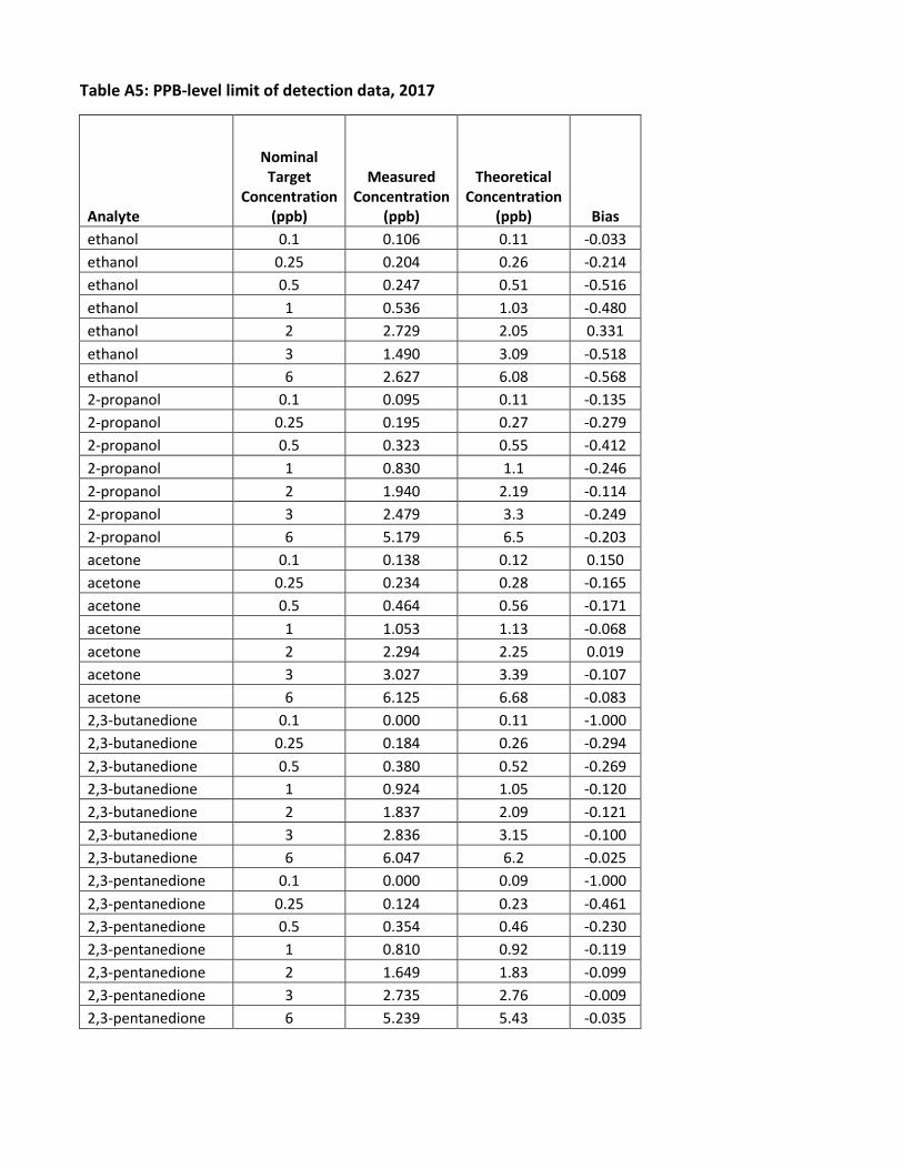
Table A5: PPB-level limit of detection data, 2017
Analyte
Nominal Target
Concentration (ppb)
Measured Concentration
(ppb)
Theoretical Concentration
(ppb)
Bias ethanol 0.1 0.106 0.11 -0.033 ethanol 0.25 0.204 0.26 -0.214 ethanol 0.5 0.247 0.51 -0.516 ethanol 1 0.536 1.03 -0.480 ethanol 2 2.729 2.05 0.331 ethanol 3 1.490 3.09 -0.518 ethanol 6 2.627 6.08 -0.568 2-propanol 0.1 0.095 0.11 -0.135 2-propanol 0.25 0.195 0.27 -0.279 2-propanol 0.5 0.323 0.55 -0.412 2-propanol 1 0.830 1.1 -0.246 2-propanol 2 1.940 2.19 -0.114 2-propanol 3 2.479 3.3 -0.249 2-propanol 6 5.179 6.5 -0.203 acetone 0.1 0.138 0.12 0.150 acetone 0.25 0.234 0.28 -0.165 acetone 0.5 0.464 0.56 -0.171 acetone 1 1.053 1.13 -0.068 acetone 2 2.294 2.25 0.019 acetone 3 3.027 3.39 -0.107 acetone 6 6.125 6.68 -0.083 2,3-butanedione 0.1 0.000 0.11 -1.000 2,3-butanedione 0.25 0.184 0.26 -0.294 2,3-butanedione 0.5 0.380 0.52 -0.269 2,3-butanedione 1 0.924 1.05 -0.120 2,3-butanedione 2 1.837 2.09 -0.121 2,3-butanedione 3 2.836 3.15 -0.100 2,3-butanedione 6 6.047 6.2 -0.025 2,3-pentanedione 0.1 0.000 0.09 -1.000 2,3-pentanedione 0.25 0.124 0.23 -0.461 2,3-pentanedione 0.5 0.354 0.46 -0.230 2,3-pentanedione 1 0.810 0.92 -0.119 2,3-pentanedione 2 1.649 1.83 -0.099 2,3-pentanedione 3 2.735 2.76 -0.009 2,3-pentanedione 6 5.239 5.43 -0.035
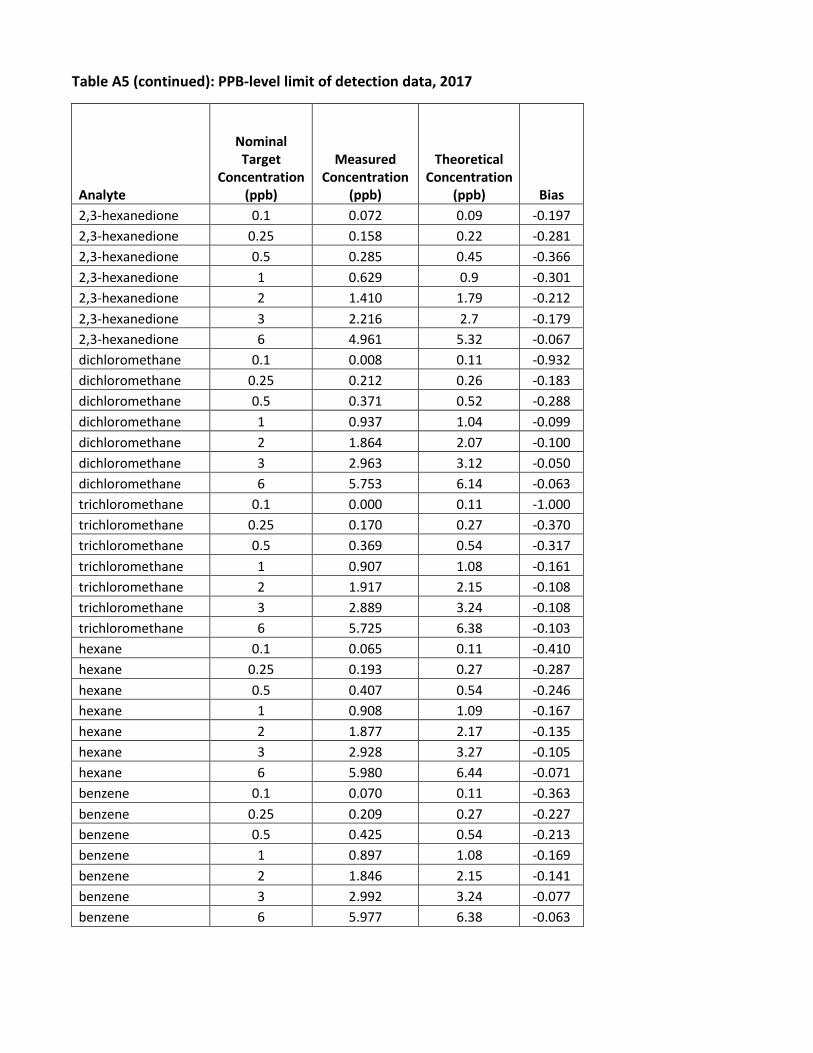
Table A5 (continued): PPB-level limit of detection data, 2017
Analyte
Nominal Target
Concentration (ppb)
Measured Concentration
(ppb)
Theoretical Concentration
(ppb)
Bias 2,3-hexanedione 0.1 0.072 0.09 -0.197 2,3-hexanedione 0.25 0.158 0.22 -0.281 2,3-hexanedione 0.5 0.285 0.45 -0.366 2,3-hexanedione 1 0.629 0.9 -0.301 2,3-hexanedione 2 1.410 1.79 -0.212 2,3-hexanedione 3 2.216 2.7 -0.179 2,3-hexanedione 6 4.961 5.32 -0.067 dichloromethane 0.1 0.008 0.11 -0.932 dichloromethane 0.25 0.212 0.26 -0.183 dichloromethane 0.5 0.371 0.52 -0.288 dichloromethane 1 0.937 1.04 -0.099 dichloromethane 2 1.864 2.07 -0.100 dichloromethane 3 2.963 3.12 -0.050 dichloromethane 6 5.753 6.14 -0.063 trichloromethane 0.1 0.000 0.11 -1.000 trichloromethane 0.25 0.170 0.27 -0.370 trichloromethane 0.5 0.369 0.54 -0.317 trichloromethane 1 0.907 1.08 -0.161 trichloromethane 2 1.917 2.15 -0.108 trichloromethane 3 2.889 3.24 -0.108 trichloromethane 6 5.725 6.38 -0.103 hexane 0.1 0.065 0.11 -0.410 hexane 0.25 0.193 0.27 -0.287 hexane 0.5 0.407 0.54 -0.246 hexane 1 0.908 1.09 -0.167 hexane 2 1.877 2.17 -0.135 hexane 3 2.928 3.27 -0.105 hexane 6 5.980 6.44 -0.071 benzene 0.1 0.070 0.11 -0.363 benzene 0.25 0.209 0.27 -0.227 benzene 0.5 0.425 0.54 -0.213 benzene 1 0.897 1.08 -0.169 benzene 2 1.846 2.15 -0.141 benzene 3 2.992 3.24 -0.077 benzene 6 5.977 6.38 -0.063
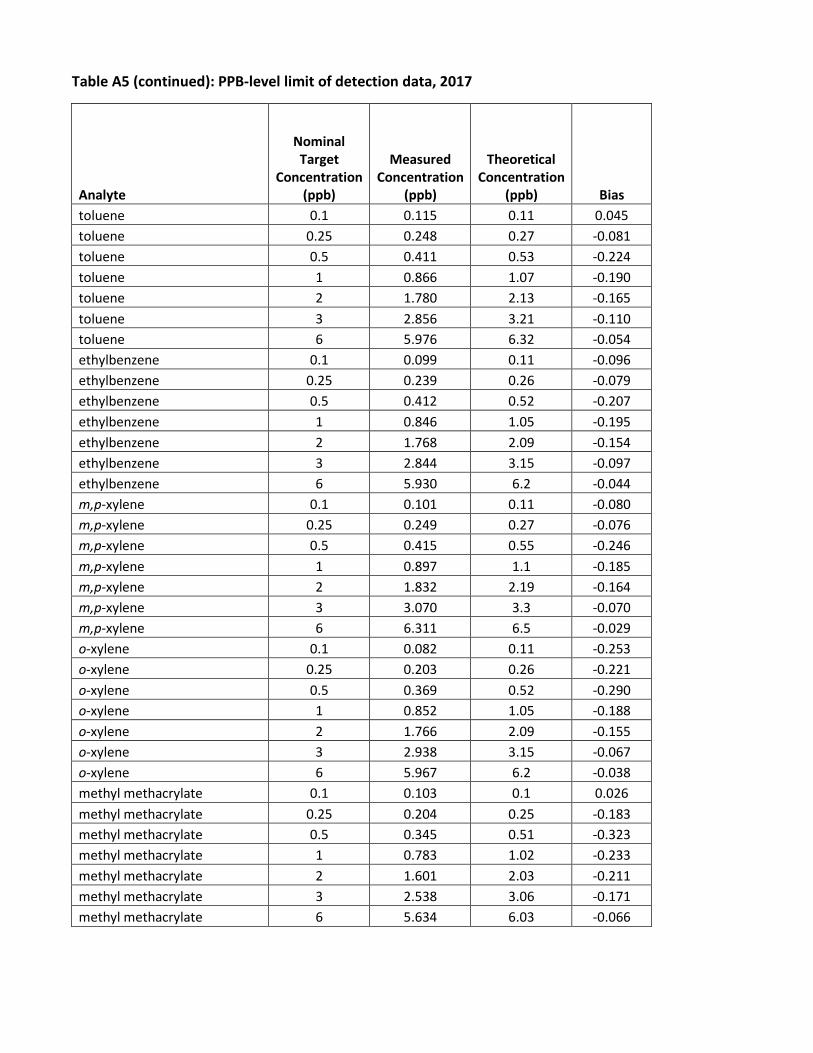
Table A5 (continued): PPB-level limit of detection data, 2017
Analyte
Nominal Target
Concentration (ppb)
Measured Concentration
(ppb)
Theoretical Concentration
(ppb)
Bias toluene 0.1 0.115 0.11 0.045 toluene 0.25 0.248 0.27 -0.081 toluene 0.5 0.411 0.53 -0.224 toluene 1 0.866 1.07 -0.190 toluene 2 1.780 2.13 -0.165 toluene 3 2.856 3.21 -0.110 toluene 6 5.976 6.32 -0.054 ethylbenzene 0.1 0.099 0.11 -0.096 ethylbenzene 0.25 0.239 0.26 -0.079 ethylbenzene 0.5 0.412 0.52 -0.207 ethylbenzene 1 0.846 1.05 -0.195 ethylbenzene 2 1.768 2.09 -0.154 ethylbenzene 3 2.844 3.15 -0.097 ethylbenzene 6 5.930 6.2 -0.044 m,p-xylene 0.1 0.101 0.11 -0.080 m,p-xylene 0.25 0.249 0.27 -0.076 m,p-xylene 0.5 0.415 0.55 -0.246 m,p-xylene 1 0.897 1.1 -0.185 m,p-xylene 2 1.832 2.19 -0.164 m,p-xylene 3 3.070 3.3 -0.070 m,p-xylene 6 6.311 6.5 -0.029 o-xylene 0.1 0.082 0.11 -0.253 o-xylene 0.25 0.203 0.26 -0.221 o-xylene 0.5 0.369 0.52 -0.290 o-xylene 1 0.852 1.05 -0.188 o-xylene 2 1.766 2.09 -0.155 o-xylene 3 2.938 3.15 -0.067 o-xylene 6 5.967 6.2 -0.038 methyl methacrylate 0.1 0.103 0.1 0.026 methyl methacrylate 0.25 0.204 0.25 -0.183 methyl methacrylate 0.5 0.345 0.51 -0.323 methyl methacrylate 1 0.783 1.02 -0.233 methyl methacrylate 2 1.601 2.03 -0.211 methyl methacrylate 3 2.538 3.06 -0.171 methyl methacrylate 6 5.634 6.03 -0.066
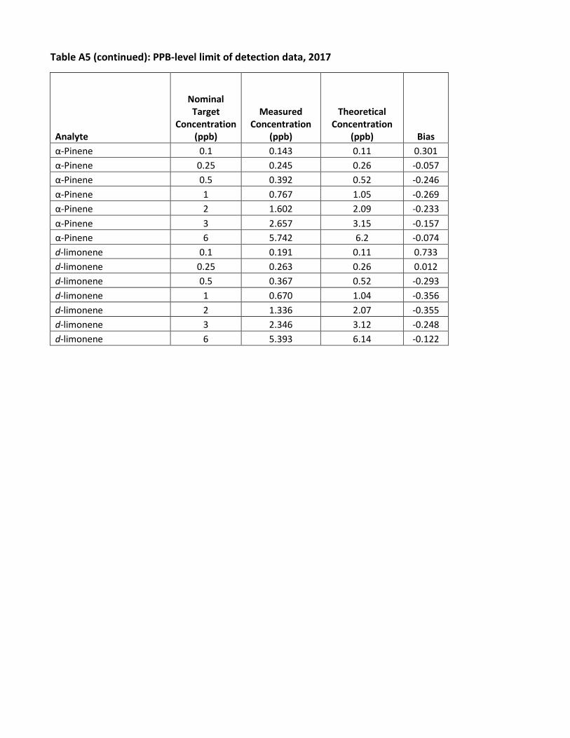
Table A5 (continued): PPB-level limit of detection data, 2017
Analyte
Nominal Target
Concentration (ppb)
Measured Concentration
(ppb)
Theoretical Concentration
(ppb)
Bias α-Pinene 0.1 0.143 0.11 0.301 α-Pinene 0.25 0.245 0.26 -0.057 α-Pinene 0.5 0.392 0.52 -0.246 α-Pinene 1 0.767 1.05 -0.269 α-Pinene 2 1.602 2.09 -0.233 α-Pinene 3 2.657 3.15 -0.157 α-Pinene 6 5.742 6.2 -0.074 d-limonene 0.1 0.191 0.11 0.733 d-limonene 0.25 0.263 0.26 0.012 d-limonene 0.5 0.367 0.52 -0.293 d-limonene 1 0.670 1.04 -0.356 d-limonene 2 1.336 2.07 -0.355 d-limonene 3 2.346 3.12 -0.248 d-limonene 6 5.393 6.14 -0.122
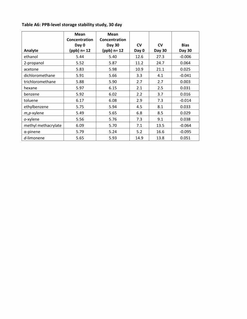
Table A6: PPB-level storage stability study, 30 day
Analyte
Mean Concentration
Day 0 (ppb) n= 12
Mean Concentration
Day 30 (ppb) n= 12
CV Day 0
CV Day 30
Bias Day 30
ethanol 5.44 5.40 12.6 27.3 -0.006 2-propanol 5.52 5.87 11.2 24.7 0.064 acetone 5.83 5.98 10.9 21.1 0.025 dichloromethane 5.91 5.66 3.3 4.1 -0.041 trichloromethane 5.88 5.90 2.7 2.7 0.003 hexane 5.97 6.15 2.1 2.5 0.031 benzene 5.92 6.02 2.2 3.7 0.016 toluene 6.17 6.08 2.9 7.3 -0.014 ethylbenzene 5.75 5.94 4.5 8.1 0.033 m,p-xylene 5.49 5.65 6.8 8.5 0.029 o-xylene 5.56 5.76 7.3 9.1 0.038 methyl methacrylate 6.09 5.70 7.1 13.5 -0.064 α-pinene 5.79 5.24 5.2 16.6 -0.095 d-limonene 5.65 5.93 14.9 13.8 0.051
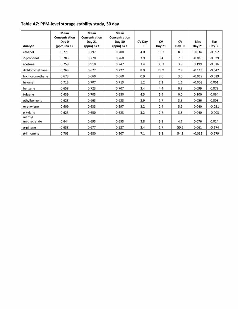
Table A7: PPM-level storage stability study, 30 day
Analyte
Mean Concentration
Day 0 (ppm) n= 12
Mean Concentration
Day 21 (ppm) n=3
Mean Concentration
Day 30 (ppm) n=3
CV Day 0
CV Day 21
CV Day 30
Bias Day 21
Bias Day 30
ethanol 0.771 0.797 0.700 4.0 16.7 8.9 0.034 -0.092
2-propanol 0.783 0.770 0.760 3.9 3.4 7.0 -0.016 -0.029
acetone 0.759 0.910 0.747 3.4 33.3 3.9 0.199 -0.016
dichloromethane 0.763 0.677 0.727 8.9 23.9 7.9 -0.113 -0.047
trichloromethane 0.673 0.660 0.660 0.9 2.6 3.0 -0.019 -0.019
hexane 0.713 0.707 0.713 1.2 2.2 1.6 -0.008 0.001
benzene 0.658 0.723 0.707 3.4 4.4 0.8 0.099 0.073
toluene 0.639 0.703 0.680 4.5 5.9 0.0 0.100 0.064
ethylbenzene 0.628 0.663 0.633 2.9 1.7 3.3 0.056 0.008
m,p-xylene 0.609 0.633 0.597 3.2 2.4 5.9 0.040 -0.021
o-xylene 0.625 0.650 0.623 3.2 2.7 3.3 0.040 -0.003 methyl methacrylate
0.644
0.693
0.653
3.8
5.8
4.7
0.076
0.014
α-pinene 0.638 0.677 0.527 3.4 1.7 50.5 0.061 -0.174
d-limonene 0.703 0.680 0.507 7.1 5.3 54.1 -0.032 -0.279
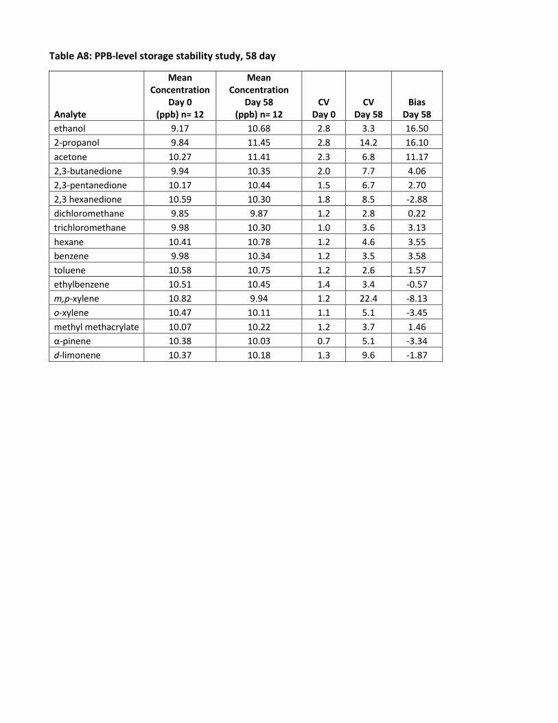
Table A8: PPB-level storage stability study, 58 day
Analyte
Mean Concentration
Day 0 (ppb) n= 12
Mean Concentration
Day 58 (ppb) n= 12
CV Day 0
CV Day 58
Bias Day 58
ethanol 9.17 10.68 2.8 3.3 16.50 2-propanol 9.84 11.45 2.8 14.2 16.10 acetone 10.27 11.41 2.3 6.8 11.17 2,3-butanedione 9.94 10.35 2.0 7.7 4.06 2,3-pentanedione 10.17 10.44 1.5 6.7 2.70 2,3 hexanedione 10.59 10.30 1.8 8.5 -2.88 dichloromethane 9.85 9.87 1.2 2.8 0.22 trichloromethane 9.98 10.30 1.0 3.6 3.13 hexane 10.41 10.78 1.2 4.6 3.55 benzene 9.98 10.34 1.2 3.5 3.58 toluene 10.58 10.75 1.2 2.6 1.57 ethylbenzene 10.51 10.45 1.4 3.4 -0.57 m,p-xylene 10.82 9.94 1.2 22.4 -8.13 o-xylene 10.47 10.11 1.1 5.1 -3.45 methyl methacrylate 10.07 10.22 1.2 3.7 1.46 α-pinene 10.38 10.03 0.7 5.1 -3.34 d-limonene 10.37 10.18 1.3 9.6 -1.87
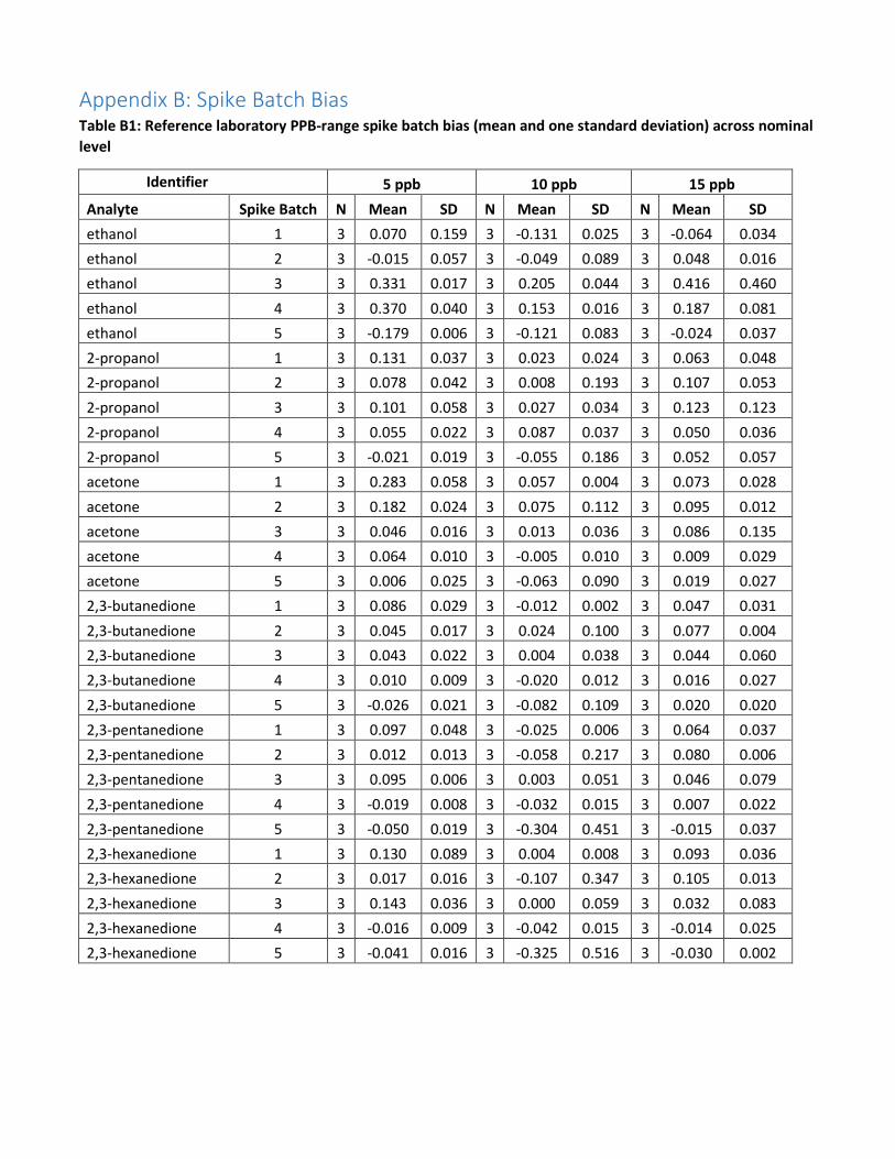
Appendix B: Spike Batch Bias Table B1: Reference laboratory PPB-range spike batch bias (mean and one standard deviation) across nominal level
Identifier 5 ppb 10 ppb 15 ppb Analyte Spike Batch N Mean SD N Mean SD N Mean SD ethanol 1 3 0.070 0.159 3 -0.131 0.025 3 -0.064 0.034 ethanol 2 3 -0.015 0.057 3 -0.049 0.089 3 0.048 0.016 ethanol 3 3 0.331 0.017 3 0.205 0.044 3 0.416 0.460 ethanol 4 3 0.370 0.040 3 0.153 0.016 3 0.187 0.081 ethanol 5 3 -0.179 0.006 3 -0.121 0.083 3 -0.024 0.037 2-propanol 1 3 0.131 0.037 3 0.023 0.024 3 0.063 0.048 2-propanol 2 3 0.078 0.042 3 0.008 0.193 3 0.107 0.053 2-propanol 3 3 0.101 0.058 3 0.027 0.034 3 0.123 0.123 2-propanol 4 3 0.055 0.022 3 0.087 0.037 3 0.050 0.036 2-propanol 5 3 -0.021 0.019 3 -0.055 0.186 3 0.052 0.057 acetone 1 3 0.283 0.058 3 0.057 0.004 3 0.073 0.028 acetone 2 3 0.182 0.024 3 0.075 0.112 3 0.095 0.012 acetone 3 3 0.046 0.016 3 0.013 0.036 3 0.086 0.135 acetone 4 3 0.064 0.010 3 -0.005 0.010 3 0.009 0.029 acetone 5 3 0.006 0.025 3 -0.063 0.090 3 0.019 0.027 2,3-butanedione 1 3 0.086 0.029 3 -0.012 0.002 3 0.047 0.031 2,3-butanedione 2 3 0.045 0.017 3 0.024 0.100 3 0.077 0.004 2,3-butanedione 3 3 0.043 0.022 3 0.004 0.038 3 0.044 0.060 2,3-butanedione 4 3 0.010 0.009 3 -0.020 0.012 3 0.016 0.027 2,3-butanedione 5 3 -0.026 0.021 3 -0.082 0.109 3 0.020 0.020 2,3-pentanedione 1 3 0.097 0.048 3 -0.025 0.006 3 0.064 0.037 2,3-pentanedione 2 3 0.012 0.013 3 -0.058 0.217 3 0.080 0.006 2,3-pentanedione 3 3 0.095 0.006 3 0.003 0.051 3 0.046 0.079 2,3-pentanedione 4 3 -0.019 0.008 3 -0.032 0.015 3 0.007 0.022 2,3-pentanedione 5 3 -0.050 0.019 3 -0.304 0.451 3 -0.015 0.037 2,3-hexanedione 1 3 0.130 0.089 3 0.004 0.008 3 0.093 0.036 2,3-hexanedione 2 3 0.017 0.016 3 -0.107 0.347 3 0.105 0.013 2,3-hexanedione 3 3 0.143 0.036 3 0.000 0.059 3 0.032 0.083 2,3-hexanedione 4 3 -0.016 0.009 3 -0.042 0.015 3 -0.014 0.025 2,3-hexanedione 5 3 -0.041 0.016 3 -0.325 0.516 3 -0.030 0.002
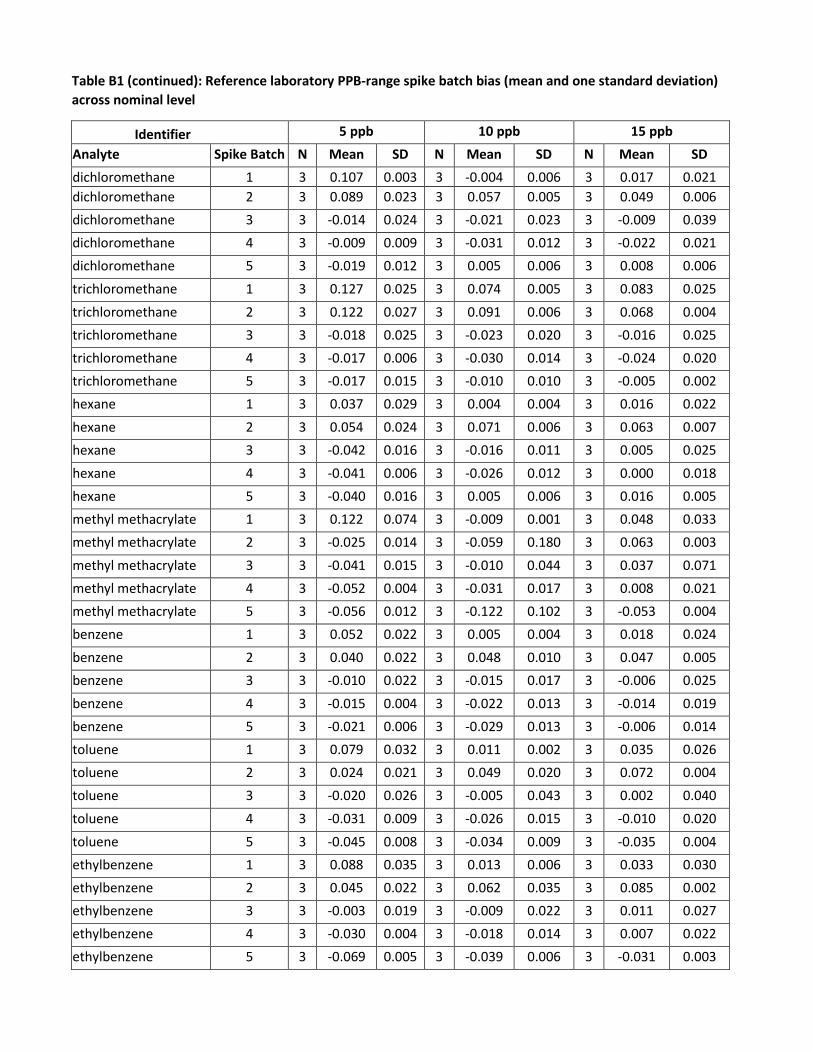
Table B1 (continued): Reference laboratory PPB-range spike batch bias (mean and one standard deviation) across nominal level
Identifier 5 ppb 10 ppb 15 ppb Analyte Spike Batch N Mean SD N Mean SD N Mean SD dichloromethane 1 3 0.107 0.003 3 -0.004 0.006 3 0.017 0.021 dichloromethane 2 3 0.089 0.023 3 0.057 0.005 3 0.049 0.006 dichloromethane 3 3 -0.014 0.024 3 -0.021 0.023 3 -0.009 0.039 dichloromethane 4 3 -0.009 0.009 3 -0.031 0.012 3 -0.022 0.021 dichloromethane 5 3 -0.019 0.012 3 0.005 0.006 3 0.008 0.006 trichloromethane 1 3 0.127 0.025 3 0.074 0.005 3 0.083 0.025 trichloromethane 2 3 0.122 0.027 3 0.091 0.006 3 0.068 0.004 trichloromethane 3 3 -0.018 0.025 3 -0.023 0.020 3 -0.016 0.025 trichloromethane 4 3 -0.017 0.006 3 -0.030 0.014 3 -0.024 0.020 trichloromethane 5 3 -0.017 0.015 3 -0.010 0.010 3 -0.005 0.002 hexane 1 3 0.037 0.029 3 0.004 0.004 3 0.016 0.022 hexane 2 3 0.054 0.024 3 0.071 0.006 3 0.063 0.007 hexane 3 3 -0.042 0.016 3 -0.016 0.011 3 0.005 0.025 hexane 4 3 -0.041 0.006 3 -0.026 0.012 3 0.000 0.018 hexane 5 3 -0.040 0.016 3 0.005 0.006 3 0.016 0.005 methyl methacrylate 1 3 0.122 0.074 3 -0.009 0.001 3 0.048 0.033 methyl methacrylate 2 3 -0.025 0.014 3 -0.059 0.180 3 0.063 0.003 methyl methacrylate 3 3 -0.041 0.015 3 -0.010 0.044 3 0.037 0.071 methyl methacrylate 4 3 -0.052 0.004 3 -0.031 0.017 3 0.008 0.021 methyl methacrylate 5 3 -0.056 0.012 3 -0.122 0.102 3 -0.053 0.004 benzene 1 3 0.052 0.022 3 0.005 0.004 3 0.018 0.024 benzene 2 3 0.040 0.022 3 0.048 0.010 3 0.047 0.005 benzene 3 3 -0.010 0.022 3 -0.015 0.017 3 -0.006 0.025 benzene 4 3 -0.015 0.004 3 -0.022 0.013 3 -0.014 0.019 benzene 5 3 -0.021 0.006 3 -0.029 0.013 3 -0.006 0.014 toluene 1 3 0.079 0.032 3 0.011 0.002 3 0.035 0.026 toluene 2 3 0.024 0.021 3 0.049 0.020 3 0.072 0.004 toluene 3 3 -0.020 0.026 3 -0.005 0.043 3 0.002 0.040 toluene 4 3 -0.031 0.009 3 -0.026 0.015 3 -0.010 0.020 toluene 5 3 -0.045 0.008 3 -0.034 0.009 3 -0.035 0.004 ethylbenzene 1 3 0.088 0.035 3 0.013 0.006 3 0.033 0.030 ethylbenzene 2 3 0.045 0.022 3 0.062 0.035 3 0.085 0.002 ethylbenzene 3 3 -0.003 0.019 3 -0.009 0.022 3 0.011 0.027 ethylbenzene 4 3 -0.030 0.004 3 -0.018 0.014 3 0.007 0.022 ethylbenzene 5 3 -0.069 0.005 3 -0.039 0.006 3 -0.031 0.003
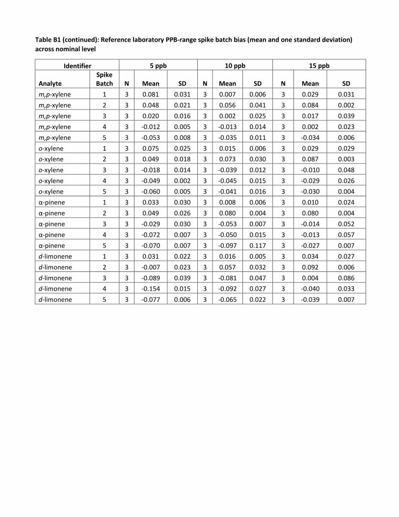
Table B1 (continued): Reference laboratory PPB-range spike batch bias (mean and one standard deviation) across nominal level
Identifier 5 ppb 10 ppb 15 ppb
Analyte Spike Batch N Mean SD N Mean SD N Mean SD
m,p-xylene 1 3 0.081 0.031 3 0.007 0.006 3 0.029 0.031 m,p-xylene 2 3 0.048 0.021 3 0.056 0.041 3 0.084 0.002 m,p-xylene 3 3 0.020 0.016 3 0.002 0.025 3 0.017 0.039 m,p-xylene 4 3 -0.012 0.005 3 -0.013 0.014 3 0.002 0.023 m,p-xylene 5 3 -0.053 0.008 3 -0.035 0.011 3 -0.034 0.006 o-xylene 1 3 0.075 0.025 3 0.015 0.006 3 0.029 0.029 o-xylene 2 3 0.049 0.018 3 0.073 0.030 3 0.087 0.003 o-xylene 3 3 -0.018 0.014 3 -0.039 0.012 3 -0.010 0.048 o-xylene 4 3 -0.049 0.002 3 -0.045 0.015 3 -0.029 0.026 o-xylene 5 3 -0.060 0.005 3 -0.041 0.016 3 -0.030 0.004 α-pinene 1 3 0.033 0.030 3 0.008 0.006 3 0.010 0.024 α-pinene 2 3 0.049 0.026 3 0.080 0.004 3 0.080 0.004 α-pinene 3 3 -0.029 0.030 3 -0.053 0.007 3 -0.014 0.052 α-pinene 4 3 -0.072 0.007 3 -0.050 0.015 3 -0.013 0.057 α-pinene 5 3 -0.070 0.007 3 -0.097 0.117 3 -0.027 0.007 d-limonene 1 3 0.031 0.022 3 0.016 0.005 3 0.034 0.027 d-limonene 2 3 -0.007 0.023 3 0.057 0.032 3 0.092 0.006 d-limonene 3 3 -0.089 0.039 3 -0.081 0.047 3 0.004 0.086 d-limonene 4 3 -0.154 0.015 3 -0.092 0.027 3 -0.040 0.033 d-limonene 5 3 -0.077 0.006 3 -0.065 0.022 3 -0.039 0.007
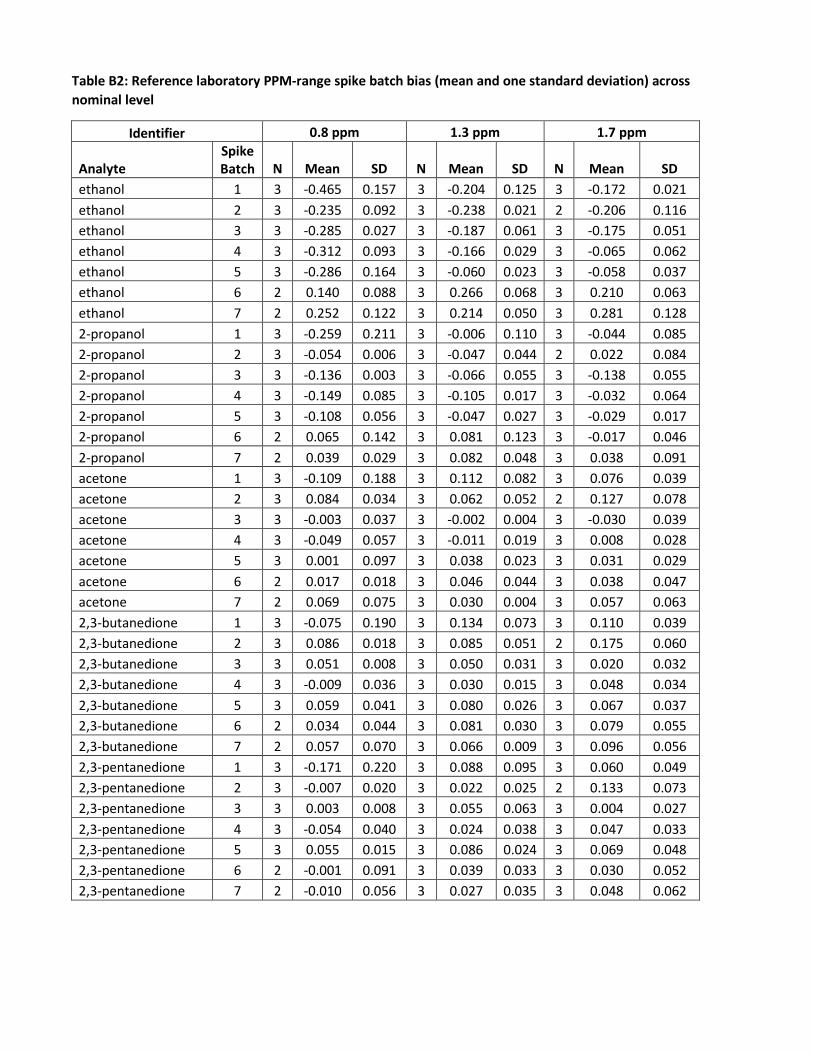
Table B2: Reference laboratory PPM-range spike batch bias (mean and one standard deviation) across nominal level
Identifier 0.8 ppm 1.3 ppm 1.7 ppm
Analyte Spike Batch N Mean SD N Mean SD N Mean SD
ethanol 1 3 -0.465 0.157 3 -0.204 0.125 3 -0.172 0.021 ethanol 2 3 -0.235 0.092 3 -0.238 0.021 2 -0.206 0.116 ethanol 3 3 -0.285 0.027 3 -0.187 0.061 3 -0.175 0.051 ethanol 4 3 -0.312 0.093 3 -0.166 0.029 3 -0.065 0.062 ethanol 5 3 -0.286 0.164 3 -0.060 0.023 3 -0.058 0.037 ethanol 6 2 0.140 0.088 3 0.266 0.068 3 0.210 0.063 ethanol 7 2 0.252 0.122 3 0.214 0.050 3 0.281 0.128 2-propanol 1 3 -0.259 0.211 3 -0.006 0.110 3 -0.044 0.085 2-propanol 2 3 -0.054 0.006 3 -0.047 0.044 2 0.022 0.084 2-propanol 3 3 -0.136 0.003 3 -0.066 0.055 3 -0.138 0.055 2-propanol 4 3 -0.149 0.085 3 -0.105 0.017 3 -0.032 0.064 2-propanol 5 3 -0.108 0.056 3 -0.047 0.027 3 -0.029 0.017 2-propanol 6 2 0.065 0.142 3 0.081 0.123 3 -0.017 0.046 2-propanol 7 2 0.039 0.029 3 0.082 0.048 3 0.038 0.091 acetone 1 3 -0.109 0.188 3 0.112 0.082 3 0.076 0.039 acetone 2 3 0.084 0.034 3 0.062 0.052 2 0.127 0.078 acetone 3 3 -0.003 0.037 3 -0.002 0.004 3 -0.030 0.039 acetone 4 3 -0.049 0.057 3 -0.011 0.019 3 0.008 0.028 acetone 5 3 0.001 0.097 3 0.038 0.023 3 0.031 0.029 acetone 6 2 0.017 0.018 3 0.046 0.044 3 0.038 0.047 acetone 7 2 0.069 0.075 3 0.030 0.004 3 0.057 0.063 2,3-butanedione 1 3 -0.075 0.190 3 0.134 0.073 3 0.110 0.039 2,3-butanedione 2 3 0.086 0.018 3 0.085 0.051 2 0.175 0.060 2,3-butanedione 3 3 0.051 0.008 3 0.050 0.031 3 0.020 0.032 2,3-butanedione 4 3 -0.009 0.036 3 0.030 0.015 3 0.048 0.034 2,3-butanedione 5 3 0.059 0.041 3 0.080 0.026 3 0.067 0.037 2,3-butanedione 6 2 0.034 0.044 3 0.081 0.030 3 0.079 0.055 2,3-butanedione 7 2 0.057 0.070 3 0.066 0.009 3 0.096 0.056 2,3-pentanedione 1 3 -0.171 0.220 3 0.088 0.095 3 0.060 0.049 2,3-pentanedione 2 3 -0.007 0.020 3 0.022 0.025 2 0.133 0.073 2,3-pentanedione 3 3 0.003 0.008 3 0.055 0.063 3 0.004 0.027 2,3-pentanedione 4 3 -0.054 0.040 3 0.024 0.038 3 0.047 0.033 2,3-pentanedione 5 3 0.055 0.015 3 0.086 0.024 3 0.069 0.048 2,3-pentanedione 6 2 -0.001 0.091 3 0.039 0.033 3 0.030 0.052 2,3-pentanedione 7 2 -0.010 0.056 3 0.027 0.035 3 0.048 0.062
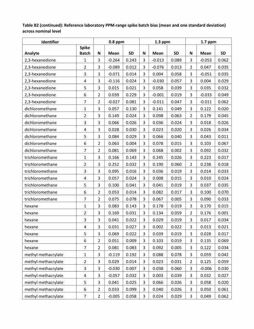
Table B2 (continued): Reference laboratory PPM-range spike batch bias (mean and one standard deviation) across nominal level
Identifier 0.8 ppm 1.3 ppm 1.7 ppm
Analyte Spike Batch N Mean SD N Mean SD N Mean SD
2,3-hexanedione 1 3 -0.264 0.243 3 -0.013 0.089 3 -0.053 0.062 2,3-hexanedione 2 3 -0.089 0.012 3 -0.076 0.013 2 0.047 0.035 2,3-hexanedione 3 3 -0.071 0.014 3 0.004 0.058 3 -0.051 0.035 2,3-hexanedione 4 3 -0.116 0.024 3 -0.030 0.057 3 0.004 0.029 2,3-hexanedione 5 3 0.015 0.021 3 0.058 0.039 3 0.035 0.032 2,3-hexanedione 6 2 0.039 0.229 3 -0.001 0.019 3 -0.033 0.049 2,3-hexanedione 7 2 -0.027 0.081 3 -0.011 0.047 3 -0.011 0.062 dichloromethane 1 3 0.057 0.130 3 0.141 0.049 3 0.122 0.020 dichloromethane 2 3 0.149 0.024 3 0.098 0.063 2 0.179 0.045 dichloromethane 3 3 0.066 0.026 3 0.036 0.024 3 0.018 0.026 dichloromethane 4 3 0.028 0.030 3 0.023 0.020 3 0.026 0.034 dichloromethane 5 3 0.084 0.029 3 0.066 0.040 3 0.043 0.011 dichloromethane 6 2 0.063 0.004 3 0.078 0.015 3 0.103 0.067 dichloromethane 7 2 0.081 0.069 3 0.068 0.002 3 0.092 0.032 trichloromethane 1 3 0.166 0.143 3 0.245 0.026 3 0.223 0.017 trichloromethane 2 3 0.252 0.032 3 0.190 0.060 2 0.238 0.018 trichloromethane 3 3 0.095 0.016 3 0.036 0.019 3 0.014 0.033 trichloromethane 4 3 0.057 0.024 3 0.008 0.015 3 0.010 0.024 trichloromethane 5 3 0.100 0.041 3 0.041 0.019 3 0.037 0.035 trichloromethane 6 2 0.053 0.014 3 0.082 0.017 3 0.100 0.070 trichloromethane 7 2 0.075 0.078 3 0.067 0.005 3 0.090 0.033 hexane 1 3 0.083 0.143 3 0.178 0.019 3 0.170 0.015 hexane 2 3 0.169 0.031 3 0.134 0.059 2 0.176 0.001 hexane 3 3 0.041 0.022 3 0.029 0.019 3 0.017 0.034 hexane 4 3 0.031 0.027 3 0.002 0.022 3 0.013 0.021 hexane 5 3 0.069 0.022 3 0.039 0.019 3 0.028 0.017 hexane 6 2 0.051 0.009 3 0.103 0.019 3 0.135 0.069 hexane 7 2 0.081 0.083 3 0.092 0.005 3 0.122 0.034 methyl methacrylate 1 3 -0.119 0.192 3 0.088 0.078 3 0.059 0.042 methyl methacrylate 2 3 0.029 0.014 3 0.023 0.031 2 0.125 0.059 methyl methacrylate 3 3 -0.030 0.007 3 0.038 0.060 3 -0.006 0.030 methyl methacrylate 4 3 -0.057 0.032 3 0.003 0.039 3 0.032 0.027 methyl methacrylate 5 3 0.041 0.025 3 0.066 0.026 3 0.058 0.020 methyl methacrylate 6 2 0.033 0.099 3 0.040 0.026 3 0.050 0.061 methyl methacrylate 7 2 -0.005 0.058 3 0.024 0.029 3 0.049 0.062
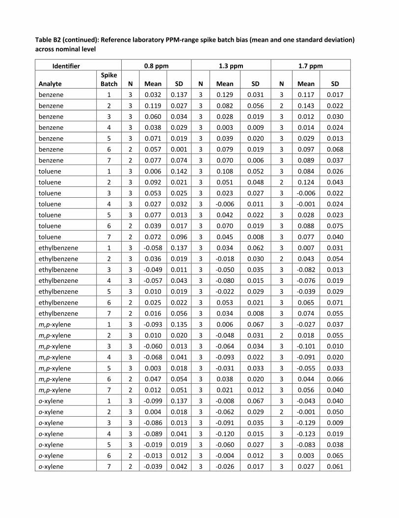
Table B2 (continued): Reference laboratory PPM-range spike batch bias (mean and one standard deviation) across nominal level
Identifier 0.8 ppm 1.3 ppm 1.7 ppm
Analyte Spike Batch N Mean SD N Mean SD N Mean SD
benzene 1 3 0.032 0.137 3 0.129 0.031 3 0.117 0.017 benzene 2 3 0.119 0.027 3 0.082 0.056 2 0.143 0.022 benzene 3 3 0.060 0.034 3 0.028 0.019 3 0.012 0.030 benzene 4 3 0.038 0.029 3 0.003 0.009 3 0.014 0.024 benzene 5 3 0.071 0.019 3 0.039 0.020 3 0.029 0.013 benzene 6 2 0.057 0.001 3 0.079 0.019 3 0.097 0.068 benzene 7 2 0.077 0.074 3 0.070 0.006 3 0.089 0.037 toluene 1 3 0.006 0.142 3 0.108 0.052 3 0.084 0.026 toluene 2 3 0.092 0.021 3 0.051 0.048 2 0.124 0.043 toluene 3 3 0.053 0.025 3 0.023 0.027 3 -0.006 0.022 toluene 4 3 0.027 0.032 3 -0.006 0.011 3 -0.001 0.024 toluene 5 3 0.077 0.013 3 0.042 0.022 3 0.028 0.023 toluene 6 2 0.039 0.017 3 0.070 0.019 3 0.088 0.075 toluene 7 2 0.072 0.096 3 0.045 0.008 3 0.077 0.040 ethylbenzene 1 3 -0.058 0.137 3 0.034 0.062 3 0.007 0.031 ethylbenzene 2 3 0.036 0.019 3 -0.018 0.030 2 0.043 0.054 ethylbenzene 3 3 -0.049 0.011 3 -0.050 0.035 3 -0.082 0.013 ethylbenzene 4 3 -0.057 0.043 3 -0.080 0.015 3 -0.076 0.019 ethylbenzene 5 3 0.010 0.019 3 -0.022 0.029 3 -0.039 0.029 ethylbenzene 6 2 0.025 0.022 3 0.053 0.021 3 0.065 0.071 ethylbenzene 7 2 0.016 0.056 3 0.034 0.008 3 0.074 0.055 m,p-xylene 1 3 -0.093 0.135 3 0.006 0.067 3 -0.027 0.037 m,p-xylene 2 3 0.010 0.020 3 -0.048 0.031 2 0.018 0.055 m,p-xylene 3 3 -0.060 0.013 3 -0.064 0.034 3 -0.101 0.010 m,p-xylene 4 3 -0.068 0.041 3 -0.093 0.022 3 -0.091 0.020 m,p-xylene 5 3 0.003 0.018 3 -0.031 0.033 3 -0.055 0.033 m,p-xylene 6 2 0.047 0.054 3 0.038 0.020 3 0.044 0.066 m,p-xylene 7 2 0.012 0.051 3 0.021 0.012 3 0.056 0.040 o-xylene 1 3 -0.099 0.137 3 -0.008 0.067 3 -0.043 0.040 o-xylene 2 3 0.004 0.018 3 -0.062 0.029 2 -0.001 0.050 o-xylene 3 3 -0.086 0.013 3 -0.091 0.035 3 -0.129 0.009 o-xylene 4 3 -0.089 0.041 3 -0.120 0.015 3 -0.123 0.019 o-xylene 5 3 -0.019 0.019 3 -0.060 0.027 3 -0.083 0.038 o-xylene 6 2 -0.013 0.012 3 -0.004 0.012 3 0.003 0.065 o-xylene 7 2 -0.039 0.042 3 -0.026 0.017 3 0.027 0.061
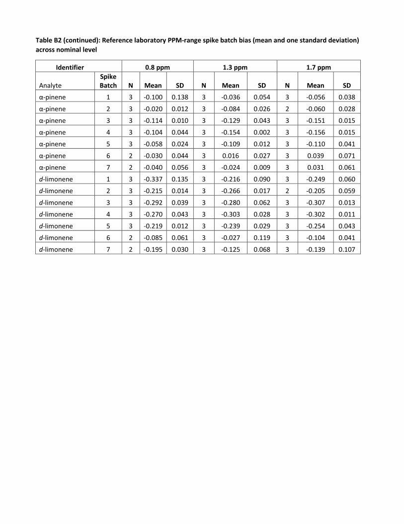
Table B2 (continued): Reference laboratory PPM-range spike batch bias (mean and one standard deviation) across nominal level
Identifier 0.8 ppm 1.3 ppm 1.7 ppm
Analyte Spike Batch N Mean SD N Mean SD N Mean SD
α-pinene 1 3 -0.100 0.138 3 -0.036 0.054 3 -0.056 0.038
α-pinene 2 3 -0.020 0.012 3 -0.084 0.026 2 -0.060 0.028
α-pinene 3 3 -0.114 0.010 3 -0.129 0.043 3 -0.151 0.015
α-pinene 4 3 -0.104 0.044 3 -0.154 0.002 3 -0.156 0.015
α-pinene 5 3 -0.058 0.024 3 -0.109 0.012 3 -0.110 0.041
α-pinene 6 2 -0.030 0.044 3 0.016 0.027 3 0.039 0.071
α-pinene 7 2 -0.040 0.056 3 -0.024 0.009 3 0.031 0.061
d-limonene 1 3 -0.337 0.135 3 -0.216 0.090 3 -0.249 0.060
d-limonene 2 3 -0.215 0.014 3 -0.266 0.017 2 -0.205 0.059
d-limonene 3 3 -0.292 0.039 3 -0.280 0.062 3 -0.307 0.013
d-limonene 4 3 -0.270 0.043 3 -0.303 0.028 3 -0.302 0.011
d-limonene 5 3 -0.219 0.012 3 -0.239 0.029 3 -0.254 0.043
d-limonene 6 2 -0.085 0.061 3 -0.027 0.119 3 -0.104 0.041
d-limonene 7 2 -0.195 0.030 3 -0.125 0.068 3 -0.139 0.107


![HPLC Method Development[1]](https://static.fdocument.org/doc/165x107/55179c7c4979599d0e8b4652/hplc-method-development1.jpg)