
New Social Collaborative Filtering Algorithms for ...For introducing a newbie like me to the world...
65
New Social Collaborative Filtering Algorithms for Recommendation on Facebook Joseph Christian G. Noel A subthesis submitted in partial fulfillment of the degree of Master of Computing (Honours) at The Department of Computer Science Australian National University October 2011
Transcript of New Social Collaborative Filtering Algorithms for ...For introducing a newbie like me to the world...
New Social Collaborative
Filtering Algorithms
for Recommendation on
Joseph Christian G. Noel
A subthesis submitted in partial fulfillment of the degree of
Master of Computing (Honours) at
The Department of Computer Science
Australian National University
October 2011

c© Joseph Christian G. Noel
Typeset in Computer Modern by TEX and LATEX 2ε.

Except where otherwise indicated, this thesis is my own original work.
Joseph Christian G. Noel
27 October 2011


To my family, who gave a 10 year old kid a 286 IBM PC running DOS back when the
only use I could think for it was listing down all my favorite Dragon Ball Z characters
on WordStar. The good old days when men were men and floppy disks were actually
floppy. And for hooking me up to the internet 3 years later, when no one else I knew
was on it, and all I did on it for months was to study deck strategies for Magic: The
Gathering. I have my passion, my career, and my future only though the unbelievable
foresight you guys had.


Acknowledgements
First of all, thanks to my adviser, Scott Sanner. For introducing a newbie like me to
the world of research, for having god-like omniscience when answering all my questions,
for being the best adviser a student could ever have, and for being a friend. I may have
already gone through all the good karma I’ll ever have in academia by having him as
my adviser on two projects for the past year and a half.
These thesis also wouldn’t be possible without the rest of the Facebook LinkR
Research Group. Thanks to Khoi-Nguyen Tran for being understanding after I crashed
his LinkR server with 8GB of RAM on two consecutive nights running my experiments,
and to Peter Christen, Lexing Xie, Edwin Bonilla and Ehsan Abbasnejad who all gave
valuable inputs on which directions these thesis should go.
Thanks my family back home, who pushed me to go back to school and get my
Masters degree even when I didn’t want to. I eventually found myself enjoying it so
much that I stayed another year. All this was possible only with their love and support.
Finally, to Aurora, who surprised me by coming to Australia the past week and
gave me enough strength to finish this. Thank you for everything.
vii

Abstract
This thesis examines the problem of designing efficient, scalable, and accurate social
collaborative filtering (CF) algorithms for personalized link recommendation on Face-
book. Unlike standard CF algorithms using relatively simple user and item features
(possibly just the user ID and link ID), link recommendation on social networks like
Facebook poses the more complex problem of learning user preferences from a rich
and complex set of user profile and interaction information. Most existing social CF
(SCF) methods have extended traditional CF matrix factorization (MF) approaches,
but have overlooked important aspects specific to the social setting; specifically, exist-
ing SCF MF methods (a) do not permit the use of item or link features in learning user
similarity based on observed interactions, (b) do not permit directly modeling user-
user information diffusion according to the social graph structure, and (c) cannot learn
that that two users may only have overlapping interests in specific areas. This thesis
proposes a unified SCF optimization framework that addresses (a)–(c) and compares
these novel algorithms with a variety of existing baslines. Evaluation is carried out
via live user trials in a custom-developed Facebook App involving data collected over
three months from over 100 App users and their nearly 30,000 friends. Not only do we
show that our novel proposals to address (a)–(c) outperform existing approaches, but
we also identify which offline ranking and classigication evaluation metrics correlate
most with human judgment of algorithm performance. Overall, this thesis represents
a critical step forward in extending SCF recommendation algorithms to fully exploit
the rich content and structure of social networks like Facebook.
ix

x
Contents
Acknowledgements vii
Abstract ix
1 Introduction 1
1.1 Objectives . . . . . . . . . . . . . . . . . . . . . . . . . . . . . . . . . . . 1
1.2 Contributions . . . . . . . . . . . . . . . . . . . . . . . . . . . . . . . . . 3
1.3 Outline . . . . . . . . . . . . . . . . . . . . . . . . . . . . . . . . . . . . 5
2 Background 7
2.1 Definitions . . . . . . . . . . . . . . . . . . . . . . . . . . . . . . . . . . . 7
2.2 Notation . . . . . . . . . . . . . . . . . . . . . . . . . . . . . . . . . . . . 8
2.3 Content-based Filtering (CBF) Algorithms . . . . . . . . . . . . . . . . 9
2.3.1 Support Vector Machines . . . . . . . . . . . . . . . . . . . . . . 9
2.4 Collaborative Filtering (CF) Algorithms . . . . . . . . . . . . . . . . . . 10
2.4.1 k-Nearest Neighbor . . . . . . . . . . . . . . . . . . . . . . . . . . 10
2.4.2 Matrix Factorization (MF) Models . . . . . . . . . . . . . . . . . 10
2.4.3 Social Collaborative Filtering . . . . . . . . . . . . . . . . . . . . 12
2.4.4 Tensor Factorization Methods . . . . . . . . . . . . . . . . . . . . 13
2.5 Summary . . . . . . . . . . . . . . . . . . . . . . . . . . . . . . . . . . . 13
3 Evaluation of Social Recommendation Systems 15
3.1 Facebook . . . . . . . . . . . . . . . . . . . . . . . . . . . . . . . . . . . 15
3.1.1 LinkR . . . . . . . . . . . . . . . . . . . . . . . . . . . . . . . . . 15
3.2 Dataset . . . . . . . . . . . . . . . . . . . . . . . . . . . . . . . . . . . . 16
3.2.1 User Data . . . . . . . . . . . . . . . . . . . . . . . . . . . . . . . 16
3.2.2 Link Data . . . . . . . . . . . . . . . . . . . . . . . . . . . . . . . 17
3.2.3 Implicit Dislikes . . . . . . . . . . . . . . . . . . . . . . . . . . . 17
3.3 Evaluation Metrics . . . . . . . . . . . . . . . . . . . . . . . . . . . . . . 17
3.4 Training and Testing Issues . . . . . . . . . . . . . . . . . . . . . . . . . 18
3.4.1 Training Data . . . . . . . . . . . . . . . . . . . . . . . . . . . . . 18
3.4.2 Live Online Recommendation Trials . . . . . . . . . . . . . . . . 19
3.4.3 Test Data . . . . . . . . . . . . . . . . . . . . . . . . . . . . . . . 19
4 Comparison of Existing Recommender Systems 21
4.1 Objective components . . . . . . . . . . . . . . . . . . . . . . . . . . . . 21
4.1.1 Matchbox Matrix Factorization (Obj pmcf ) . . . . . . . . . . . . . 22
4.1.2 L2 U Regularization (Obj ru) . . . . . . . . . . . . . . . . . . . . 22
xi
xii Contents
4.1.3 L2 V Regularization (Obj rv ) . . . . . . . . . . . . . . . . . . . . 22
4.1.4 Social Regularization (Obj rs) . . . . . . . . . . . . . . . . . . . . 22
4.1.5 Derivatives . . . . . . . . . . . . . . . . . . . . . . . . . . . . . . 23
4.2 Algorithms . . . . . . . . . . . . . . . . . . . . . . . . . . . . . . . . . . 25
4.3 Online Results . . . . . . . . . . . . . . . . . . . . . . . . . . . . . . . . 25
4.4 Survey Results . . . . . . . . . . . . . . . . . . . . . . . . . . . . . . . . 26
4.5 Offline Results . . . . . . . . . . . . . . . . . . . . . . . . . . . . . . . . 28
4.6 Summary . . . . . . . . . . . . . . . . . . . . . . . . . . . . . . . . . . . 29
5 New Algorithms for Social Recommendation 33
5.1 New Objective Components . . . . . . . . . . . . . . . . . . . . . . . . . 33
5.1.1 Hybrid Objective (Obj phy ) . . . . . . . . . . . . . . . . . . . . . 33
5.1.2 L2 w Regularization (Obj rw ) . . . . . . . . . . . . . . . . . . . . 34
5.1.3 Social Spectral Regularization (Obj rss) . . . . . . . . . . . . . . . 34
5.1.4 Social Co-preference Regularization (Obj rsc) . . . . . . . . . . . 35
5.1.5 Social Co-preference Spectral Regularization (Obj rscs) . . . . . . 35
5.1.6 Derivatives . . . . . . . . . . . . . . . . . . . . . . . . . . . . . . 36
5.2 Second Trial . . . . . . . . . . . . . . . . . . . . . . . . . . . . . . . . . . 39
5.2.1 Online Results . . . . . . . . . . . . . . . . . . . . . . . . . . . . 39
5.3 Offline Results . . . . . . . . . . . . . . . . . . . . . . . . . . . . . . . . 42
5.4 Summary . . . . . . . . . . . . . . . . . . . . . . . . . . . . . . . . . . . 43
6 Conclusion 47
6.1 Summary . . . . . . . . . . . . . . . . . . . . . . . . . . . . . . . . . . . 47
6.2 Future Work . . . . . . . . . . . . . . . . . . . . . . . . . . . . . . . . . 48
Bibliography 51
Chapter 1
Introduction
Given the vast amount of content available on the Internet, finding information of
personal interest (news, blogs, videos, movies, books, etc.) is often like finding a
needle in a haystack. Recommender systems based on collaborative filtering (CF) aim
to address this problem by leveraging the preferences of a user population under the
assumption that similar users will have similar preferences. These principles underlie
the recommendation algorithms powering websites like Amazon and Netflix.1
As the web has become more social with the emergence of Facebook, Twitter,
LinkedIn, and most recently Google+, this adds myriad new dimensions to the recom-
mendation problem by making available a rich labeled graph structure of social content
from which user preferences can be learned and new recommendations can be made.
In this socially connected setting, no longer are web users simply described by an IP
address (with perhaps associated geographical information and browsing history), but
rather they are described by a rich user profile (age, gender, location, educational and
work history, preferences, etc.) and a rich history of user interactions with their friends
(comments/posts, clicks of like, tagging in photos, mutual group memberships, etc.).
This rich information poses both an amazing opportunity and a daunting challenge for
machine learning methods applied to social recommendation — how do we fully exploit
the social network content in recommendation algorithms?
1.1 Objectives
This thesis examines the problem of designing efficient, scalable, and accurate social CF
(SCF) algorithms for personalized link recommendation on Facebook – quite simply the
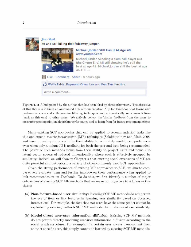
task of recommending personalized links to users that might interest them. We show
an example link posted on Facebook in Figure 1.1 that we might wish to recommend to
a subset of users; once link recommendations such as this one are made, we then need
to gather feedback from users in order to (a) learn to make better recommendations in
the future and (b) to evaluate the efficacy of our different recommendation approaches.
1On Amazon, this is directly evident with statements displayed of the form “users who looked atitem X ended up purchasing item Y 90% of the time”. While the exact inner workings of Netflix arenot published, the best performing recommendation algorithm in the popular Netflix prize competi-tion [Toscher and Jahrer 2009] used an ensemble of CF methods.
1
2 Introduction
Figure 1.1: A link posted by the author that has been liked by three other users. The objective
of this thesis is to build an automated link recommendation App for Facebook that learns user
preferences via social collaborative filtering techniques and automatically recommends links
(such as this one) to other users. We actively collect like/dislike feedback from the users to
measure recommendation algorithm performance and to learn from for future recommendations.
Many existing SCF approaches that can be applied to recommendation tasks like
this one extend matrix factorization (MF) techniques [Salakhutdinov and Mnih 2008]
and have proved quite powerful in their ability to accurately model user preferences
even when only a unique ID is available for both the user and item being recommended.
The power of such methods stems from their ability to project users and items into
latent vector spaces of reduced dimensionality where each is effectively grouped by
similarity. Indeed, we will show in Chapter 4 that existing social extensions of MF are
quite powerful and outperform a variety of other commonly used SCF approaches.
Given the strong performance of existing MF approaches to SCF, we aim to com-
paratively evaluate them and further improve on their performance when applied to
link recommendation on Facebook. To do this, we first identify a number of major
deficiencies of existing SCF MF methods that we make our objective to address in this
thesis:
(a) Non-feature-based user similarity: Existing SCF MF methods do not permit
the use of item or link features in learning user similarity based on observed
interactions. For example, the fact that two users have the same gender cannot be
exploited by existing methods SCF MF methods that make use of user similarity.
(b) Model direct user-user information diffusion: Existing SCF MF methods
do not permit directly modeling user-user information diffusion according to the
social graph structure. For example, if a certain user always likes content from
another specific user, this simply cannot be learned by existing SCF MF methods.
§1.2 Contributions 3
(c) Restricted common interests: Existing SCF MF methods cannot learn from
the fact that two users have common overlapping interests in specific areas. For
example, a friend and their co-worker may both like the same links regarding
technical content, but have differing interests when it comes to politically-oriented
links — knowing this would allow one to recommend technical content posted by
one user to the other, but existing SCF methods cannot explicitly encourage this.
This thesis addresses all of these problems with novel contributions in an efficient,
scalable, and unified latent factorization component framework for SCF. We present
results of our algorithms on live trials in a custom-developed Facebook App involving
data collected over three months from over 100 App users and their nearly 30,000
friends. These results show that a number of extensions proposed to resolve (a)–(c)
outperform all previously existing algorithms.
In addition, given that live online user evaluation trials are time-consuming, requir-
ing many users and often an evaluation period of at least one month, we have one last
important objective to address in this thesis:
(d) Identifying passive evaluation paradigms that correlate with actively
elicited human judgments. The benefits of doing this are many-fold. When
designing new SCF algorithms, there are myriad design choices to be made, for
which actual performance evaluation is the only way to validate the correct choice.
Furthermore, simple parameter tuning is crucial for best performance and SCF
algorithms are often highly sensitive to well-tuned parameters. Thus for the
purpose of algorithm design and tuning, it is crucial to have methods and metrics
that can be evaluated immediately on passive data (i.e., a passive data set of user
likes) that are shown to correlate with human judgments in order to avoid the
time-consuming process of evaluating the algorithms in live human trials.
1.2 Contributions
In the preceding section, we outlined three deficiencies of existing MF approaches for
SCF. Now we discuss our specific contributions in this thesis to address these three
deficiencies:
(a) User-feature social regularization: One can encode prior knowledge into the
learning process using a technique known as regularization. In the case of social
MF, we often want to regularize the learned latent representations of users to
enforce that users who interact heavily often have similar preferences, and hence
similar latent representations.
Thus to address the deficiency noted in non-feature-based user similarity, we build
on ideas used in Matchbox [Stern et al. 2009] to incorporate user features into the
social regularization objective for SCF. There are two commonly used methods
for social regularization in SCF — in Chapter 5 we extend both to handle user
features and determine that the spectral regularization extension performs best.
4 Introduction
(b) Hybrid social collaborative filtering: While MF methods prove to be excel-
lent at projecting user and items into latent spaces, they suffer from the caveat
that they cannot model joint features over user and items (they can only work
with independent user features and independent item features). This is problem-
atic when it comes to the issue of modeling direct user-user information diffusion
— in short, the task of learning how often information flows from one specific
user to another specific user.
The remedy for this turns out to be quite simple — we need only introduce an
objective component in addition to the standard MF objective that serves as a
simple linear regressor for such information diffusion observations. Because the
resulting objective is a combination of latent MF and linear regression objectives,
we refer to it simply as hybrid SCF. In Chapter 5, we evaluate this approach and
show that it outperforms standard SCF.
(c) Copreference regularization: Existing SCF methods that employ social reg-
ularization make a somewhat coarse assumption that if two users interact heavily
(or even worse, are simply friends) that their latent representations must match
as closely as possible. Considering that friends have different reasons for their
friendships — co-worders, schoolmates, common hobby — it is reasonable to ex-
pect that two people (friends or not) may only share restricted common interests:
co-workers may both enjoy technical content related to work, but differ otherwise;
schoolmates may like to hear news about other schoolmates, but differ otherwise;
people who share an interest in a common hobby are obviously interested in that
hobby, but should not necessarily share common interests elsewhere.
To this end, we propose a finer-grained approach to regularizing users by restrict-
ing their latent user representation to be similar (or different) only in subspaces
relevant to the items mutually liked/disliked (or disagreed upon – one user likes
and the other dislikes). Because this method of regularization requires evidence
of preferences between two users for the same item, we refer to it as regularizing
based on copreferences. In Chapter 5, we evaluate this extension to standard
SCF and show that it improves performance.
The previous contributions all relate to algorithmic and machine learning aspects
of SCF algorithms. However, in a different dimension and as discussed in the previous
section, we also have to know how to evaluate these algorithms both from active user
feedback (ratings of new recommendations) and passive user content (simply a cato-
logue of previously rated links for a user). Thus as our final contribution, we perform
the following extensive comparative evaluation:
(d) Comparative evaluation of active and passive metrics that align with
user judgments: In Chapter 3, we propose a number of training and testing
regimes and a number of evaluation metrics for both ranking and classification
paradigms. In both Chapters 4 and Chapters 5, we compare the performance
of these metrics with the given algorithms and raw data in order to determine
§1.3 Outline 5
which regimes and metrics correlate closely with human judgment of performance
in each setting.
1.3 Outline
The remaining chapters in this thesis are organized as follows:
• Chapter 2: We first define notation used throughout the thesis and then pro-
ceed to review both standard collaborative filtering approaches, specific MF ap-
proaches, and their social extensions.
• Chapter 3: We discuss the specific details of our Facebook link recommenda-
tion application and then our evaluation methodology for both offline and online
(live user trial) experimentation. Our goal here is to evaluate a variety of perfor-
mance objectives, both qualitative and quantitative, in order to evaluate the user
experience with each recommendation algorithm and to determine which online
evaluations correlate with which offline evaluations.
• Chapter 4: We empirically investigate existing SCF methods in our Facebook
App and evaluation framework. Our objective here is to carry out a fair com-
parison and understand the settings in which each algorithm works — and most
importantly for research progress — where these algorithms can be improved.
• Chapter 5: We begin by discussing novel algorithms that we propose along
the lines of our contributions outlined in this Introduction. Then proceed to
evaluate them in our Facebook App and evaluation framework to understand
whether these improve over the baselines, as well as to understand if there are
any obvious deficiencies in the new approaches.
• Conclusions: We summarize our conclusions from this work and outline direc-
tions for future research.
All combined, this thesis represents a critical step forward in SCF algorithms based
on top-performing MF methods and their ability to fully exploit the breadth of infor-
mation available on social networks to achieve state-of-the-art link recommendation.

6 Introduction
Chapter 2
Background
In the following, we outline the high-level ideas behind recommender systems — sys-
tems whose task is to adapt to user preferences in order to recommend items that
the user may like. Following a general discussion of techniques, we proceed to de-
fine mathematical notation used throughout the thesis along with a mathematically
detailed discussion of various published techniques for recommender systems that we
either compare to or extend in this thesis.
2.1 Definitions
There are two general approaches to recommender systems. The first is known as
content-based filtering (CBF), which makes individual recommendations based on cor-
relations between the item features of those items the user has explicitly liked and
similar items that the system could potentially recommend; in practice CBF is simply
the machine learning tasks of classification (will the user like a certain item?) or re-
gression (how much will they like it?). The second approach is collaborative filtering
(CF) [Resnick and Varian 1997], which is defined as the task of predicting whether a
user will like (or dislike) an item by using that user’s preferences as well as those of
other users. In general, CBF requires item features whereas CF requires multiple users
in order to work.1
Our thesis work takes CF one step further than its traditional use [Resnick and
Varian 1997] in that we assume we are recommending in the context of a social network.
We loosely define social CF (SCF) as the task of CF augmented with additional social
network information such as the following that are available on social networking sites
such as Facebook:
• Expressive personal profile content: gender, age, places lived, schools attended;
favorite books, movies, quotes; online photo albums (and associated comment
text).
• Explicit friendship or trust relationships.
1In this thesis we use item features (CBF) and user features in conjunction with CF. Since our ideasare mainly driven by CF extended to use item and user features, we generally refer to all of our newlyproposed methods in this thesis as CF even when they are actually hybrid CF+CBF methods.
7
8 Background
• Content that users have personally posted (often text and links).
• Content of interactions between users (often text and links).
• Evidence of other interactions between users (being tagged in photos).
• Publicly available preferences (likes/dislikes of posts and links).
• Publicly available group memberships (often for hobbies, activities, social or po-
litical discussion).
We note that CF is possible in a social setting without taking advantage of the above
social information, nonetheless we refer to any CF method that can be applied in a
social setting as SCF.
2.2 Notation
Here we outline mathematical notation common to the SCF setting and models ex-
plored in this thesis:
• N users. For methods that can exploit user features, we define an I-element
user feature vector x ∈ RI (alternately if a second user is needed, z ∈ RI). For
methods that do not use user feature vectors, we simply assume x is an index
x ∈ {1 . . . N} and that I = N .
• M items. For methods that can exploit item features, we define a J-element
feature vector y ∈ RJ . The feature vectors for users and items can consist of
any real-valued features as well as {0, 1} features like user and item IDs. For
methods that do not use item feature vectors, we simply assume y is an index
y ∈ {1 . . .M} and that J = M .
• A (non-exhaustive) data setD of single user preferences of the formD = {(x,y)→Rx,y} where the binary response R is represented by Rx,y ∈ {0 (dislike), 1 (like)}.
• A (non-exhaustive) data set C of co-preferences (cases where both users x and
z expressed a preference for y – not necessarily in agreement) derived from
D of the form C = {(x, z,y) → Px,z,y} where co-preference class Px,z,y ∈{−1 (disagree), 1 (agree)}. Intuitively, if both user x and z liked or disliked
item y then we say they agree, otherwise if one liked the item and the other
disliked it, we say they disagree.
• A similarity rating Sx,z between any users x and z. This is used to summarize all
social interaction between user x and user z in the term Sx,z ∈ R. A definition
of Sx,z ∈ R that has been useful is the following:
Intx,z =# interactions between x and z
average # interactions between all user pairs(2.1)
Sx,z = ln (Intx,z) (2.2)

§2.3 Content-based Filtering (CBF) Algorithms 9
The interactions between users that we include to define Intx,z are:
1. Being friends on Facebook
2. Posting an item (link, photo, video, photo, or message) on a user’s wall.
3. Liking an item (link, photo, video, photo, or message) on a user’s wall.
4. Commenting on an item (link, photo, video, photo, or message) on a user’s
wall.
5. Being tagged together in the same photo.
6. Being tagged together in the same video.
7. Two users tagging themselves as attending the same school.
8. Two users tagging themselves as attending the same class in school.
9. Two users tagging themselves as playing sports together.
10. Two users tagging themselves as working together for the same company.
11. Two users tagging themselves as working together on the same project for
the same company.
In addition, we can define S+x,z, a non-negative variant of Sx,z:
S+x,z = ln (1 + Intx,z) (2.3)
Having now defined all notation, we proceed to a discussion of CF algorithms
compared to or extended in this thesis.
2.3 Content-based Filtering (CBF) Algorithms
As noted previously, CBF methods can be viewed as classification or regression ap-
proaches. Since our objective here is to classify whether a user likes an item or not
(i.e., a classification objective), we focus on classification CBF approaches in this thesis.
For an initial evaluation, perhaps the most well-known and generally top-performing
classifier is the support vector machine, hence it is the CBF approach we choose to
compare to in this work.
2.3.1 Support Vector Machines
A support vector machine (SVM) [Cortes and Vapnik 1995] is a type of supervised
learning algorithm for classification based on finding optimal separating hyperplanes
in a possibly high-dimensional feature space. During training, an SVM builds a model
by constructing a set of hyperplanes that separates one class of data from another class
with the maximum margin possible. Data are classified by finding out on which side
of a hyperplane they fall on.
For the experiments in this thesis, the SVM uses a fixed-length feature vector f ∈ RFderived from the (x,y) ∈ D, denoted as fx,y. In general, fx,y may include features that
10 Background
are non-zero only for specific items and/or users, e.g., a {0, 1} indicator feature that
user x and user z have both liked item y. Specific features used in the SVM for the
Facebook link recommendation task are defined in Section 3.2.
The SVM implementation used for this thesis is LibSVM [Chang and Lin 2001],
which provides a regression score on the classification (i.e., the non-thresholded learned
linear function) which can be used for ranking the results.
2.4 Collaborative Filtering (CF) Algorithms
2.4.1 k-Nearest Neighbor
One of the most common forms of CF is the nearest neighbor approach [Bell and Koren
2007]. The k-nearest neighbor algorithm is a method of classification or regression that
is based on finding the k-closest training data neighbors in the feature space nearest
to a target point and combining the information from these neighbors — perhaps in
a weighted manner — to determine the classification or regression value for the target
point.
There are two main variants of nearest neighbors for collaborative recommendation,
user-based and item-based — both methods generally assume that no user or item
features are provided, so here x and y are simply respective user and item indices.
Given a user x and an item y, let N(x : y) be the set of user nearest neighbors of x
that have also given a rating for y, let N(y : x) be the set of item nearest neighbors of
y that have also been rated by x, let Sx,z some measure of similarity rating between
users x and z (as defined previously), and let Sy,y′ be some measure of similarity rating
for items y and y′. Following [Bell and Koren 2007], the predicted rating Rx,y ∈ [0, 1]
that the user x gives item y can then be calculated in one of two ways:
• User-based similarity:
Rx,y =
∑z∈N(x:y) Sx,zRz,y∑
z∈N(x:y) Sx,z
• Item-based similarity:
Rx,y =
∑y′∈N(y:x) Sy,y′Rx,y′∑
y′∈N(y:x) Sy,y′
The question of which approach to use depends on the dataset. When the number
of items is far fewer than the number of users, it has been found that the item-based
approach usually provides better predictions as well as being more efficient in compu-
tations [Bell and Koren 2007].
2.4.2 Matrix Factorization (MF) Models
As done in standard CF methods, we assume that a matrix U allows us to project users
x (and z) into a latent space of dimensionality K; likewise we assume that a matrix V
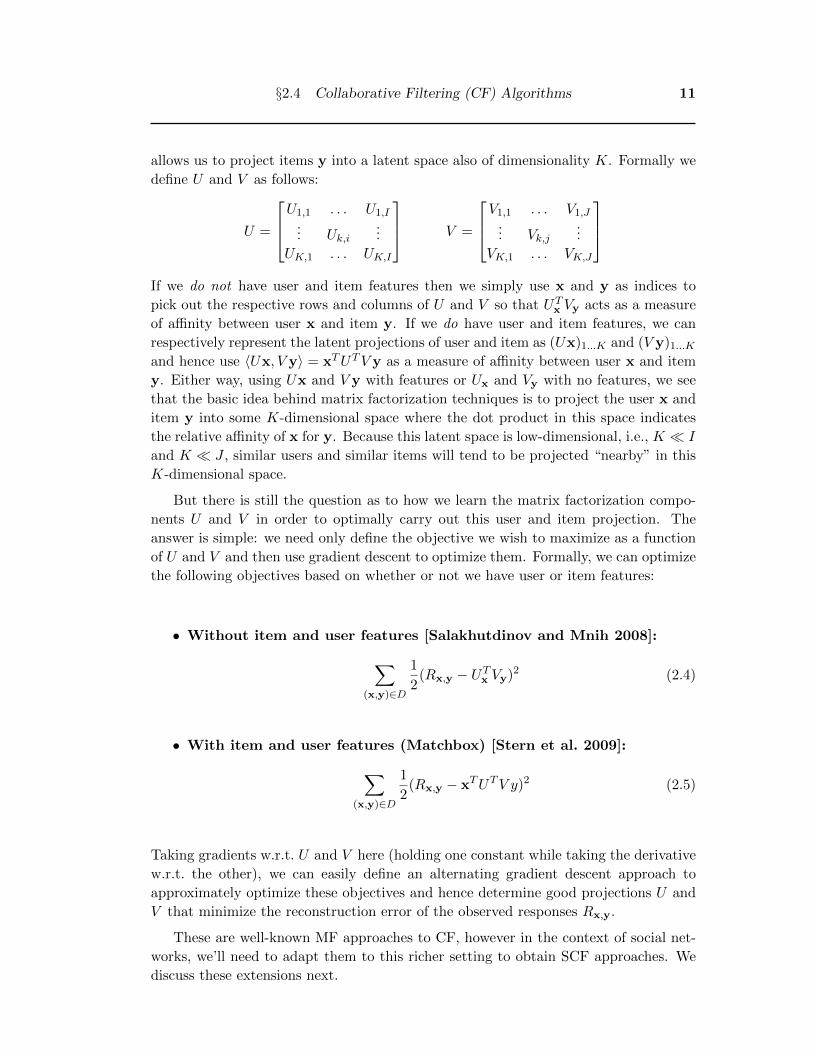
§2.4 Collaborative Filtering (CF) Algorithms 11
allows us to project items y into a latent space also of dimensionality K. Formally we
define U and V as follows:
U =
U1,1 . . . U1,I... Uk,i
...
UK,1 . . . UK,I
V =
V1,1 . . . V1,J... Vk,j
...
VK,1 . . . VK,J
If we do not have user and item features then we simply use x and y as indices to
pick out the respective rows and columns of U and V so that UTx Vy acts as a measure
of affinity between user x and item y. If we do have user and item features, we can
respectively represent the latent projections of user and item as (Ux)1...K and (V y)1...Kand hence use 〈Ux, V y〉 = xTUTV y as a measure of affinity between user x and item
y. Either way, using Ux and V y with features or Ux and Vy with no features, we see
that the basic idea behind matrix factorization techniques is to project the user x and
item y into some K-dimensional space where the dot product in this space indicates
the relative affinity of x for y. Because this latent space is low-dimensional, i.e., K � I
and K � J , similar users and similar items will tend to be projected “nearby” in this
K-dimensional space.
But there is still the question as to how we learn the matrix factorization compo-
nents U and V in order to optimally carry out this user and item projection. The
answer is simple: we need only define the objective we wish to maximize as a function
of U and V and then use gradient descent to optimize them. Formally, we can optimize
the following objectives based on whether or not we have user or item features:
• Without item and user features [Salakhutdinov and Mnih 2008]:∑(x,y)∈D
1
2(Rx,y − UTx Vy)2 (2.4)
• With item and user features (Matchbox) [Stern et al. 2009]:∑(x,y)∈D
1
2(Rx,y − xTUTV y)2 (2.5)
Taking gradients w.r.t. U and V here (holding one constant while taking the derivative
w.r.t. the other), we can easily define an alternating gradient descent approach to
approximately optimize these objectives and hence determine good projections U and
V that minimize the reconstruction error of the observed responses Rx,y.
These are well-known MF approaches to CF, however in the context of social net-
works, we’ll need to adapt them to this richer setting to obtain SCF approaches. We
discuss these extensions next.
12 Background
2.4.3 Social Collaborative Filtering
There are essentially two general classes of MF methods applied to SCF that we discuss
below. All of the social MF methods defined to date do not make use of user or item
features and hence x and z below should be treated as user indices as defined previously
for the non-feature case.
The first class of social MF methods can be termed as social regularization ap-
proaches in that they somehow constrain the latent projection represented by U .
There are two social regularization methods that directly constrain U for user x
and z based on evidence Sx,z of interaction between x and z. We call these methods:
• Social regularization [Yang et al. 2011; Cui et al. 2011]:∑ ∑z∈friends(x)
1
2(Sx,z − 〈Ux, Uz〉)2
• Social spectral regularization [Ma et al. 2011; Li and Yeung 2009]:∑i
∑z∈friends(x)
1
2S+x,z‖Ux − Uz‖22
We refer to the latter as spectral regularization methods since they are identical to the
objectives used in spectral clustering [Ng et al. 2001].
The SoRec system [Ma et al. 2008] proposes a slight twist on social spectral regu-
larization in that it learns a third N×N (n.b., I = N) interactions matrix Z, and uses
UTz Zz to predict user-user interaction preferences in the same way that standard CF
uses V in UTx Vy to predict user-item ratings. SoRec also uses a sigmoidal transform
σ(o) = 11+e−o on the predictions:
• SoRec regularization [Ma et al. 2008]:
∑z
∑z∈friends(x)
1
2(Sx,z − σ(〈Ux, Zz〉))2
The second class of SCF MF approaches represented by the single examplar of
the Social Trust Ensemble can be termed as a weighted average approach since this
approach simply composes a prediction for item y from a weighted average of a user
x’s predictions as well as their friends (z) predictions (as evidenced by the additional∑z in the objective below):
• Social Trust Ensemble [Ma et al. 2009] (Non-spectral):∑(x,y)∈D
1
2(Rx,y − σ(UTx Vy +
∑k
UTx Vz))2
§2.5 Summary 13
As for the MF CF methods, all MF SCF methods can be optimized by alternating
gradient descent on the respective matrix parameterizations.
2.4.4 Tensor Factorization Methods
On a final note, we observe that Tensor factorization (TF) methods can be used to
learn latent models of interaction of 2 dimensions and higher. A 2-dimensional TF
method is simply standard MF. An example of a 3-dimensional TF method is given
by [Rendle et al. 2009], where recommendation of user-specific tags for an item are
modeled with tags, user, and items each in one dimension. To date, TF methods
have not been used for social recommendation, however, we will draw on the idea of
using additional (more than 2) dimensions of latent learning in some of our novel SCF
approaches in Chapter 5.
2.5 Summary
In this chapter we have seen some of the different existing methods for CF and SCF.
Each of these methods has its own weaknesses, some of which we detailed in Chapter
1. Next, we discuss how we evaluate these existing CF and SCF algorithms on the
task of link recommendation on Facebook; following this, we proceed in subsequent
chapters to evaluate these algorithms as well as propose novel algorithms that extend
the background work covered here.

14 Background
Chapter 3
Evaluation of Social
Recommendation Systems
In this chapter we first discuss our Facebook Link Recommendation (LinkR) applica-
tion and then proceed to discuss how it can be evaluated using general principles of
evaluation used in the machine learning and information retrieval fields.
3.1 Facebook
Facebook is a social networking service that is currently the largest in the world. As of
July 2011 it had more that 750 million active users. Users in Facebook create a profile
and establish “friend” connections between users to establish their social network. Each
user has a “Wall” where they and their friends can make posts to. These posts can
be links, photos, status updates, etc. Items that have been posted by a user can be
“liked”, shared, or commented upon by other users. An example of a link post on a
Wall that had been liked by others was provided previously in Figure 1.1.
This thesis seeks to find out how best to recommend links to individual users such
that there is a high likelihood that they will “like” their recommended links. We do this
by creating a Facebook application (i.e., ‘Facebook “App”) that recommends links to
users everyday, where the users may give their feedback on the links indicating whether
they liked it or disliked it. We discuss this application in detail next.
3.1.1 LinkR
Facebook allows applications to be developed that can be installed by their users.
As part of this thesis project, the LinkR Facebook application was developed.1 The
functionalities of the LinkR application are as follows:
1. Collect data that have been shared by users and their friends on Facebook.
2. Recommend (three) links to the users daily.
1The main developer of the LinkR Facebook App is Khoi-Nguyen Tran, a PhD student at theAustralian National University. Khoi-Nguyen wrote the user interface and database crawling code forLinkR. All of the learning and recommendation algorithms used by LinkR were written solely by theauthor for the purpose of this thesis.
15
16 Evaluation of Social Recommendation Systems
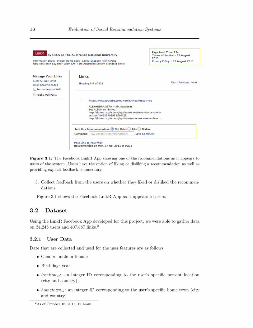
Figure 3.1: The Facebook LinkR App showing one of the recommendations as it appears to
users of the system. Users have the option of liking or disliking a recommendation as well as
providing explicit feedback commentary.
3. Collect feedback from the users on whether they liked or disliked the recommen-
dations.
Figure 3.1 shows the Facebook LinkR App as it appears to users.
3.2 Dataset
Using the LinkR Facebook App developed for this project, we were able to gather data
on 34,245 users and 407,887 links.2
3.2.1 User Data
Date that are collected and used for the user features are as follows:
• Gender: male or female
• Birthday: year
• location id : an integer ID corresponding to the user’s specific present location
(city and country)
• hometown id : an integer ID corresponding to the user’s specific home town (city
and country)
2As of October 18, 2011, 12:15am.

§3.3 Evaluation Metrics 17
• Fx,z ∈ {0, 1}: indicator of whether users x and z are friends.
• Intx,z ∈ N: interactions on Facebook between users x and z as defined in Sec-
tion 2.2.
3.2.2 Link Data
Data that are used for the link features are:
• id of the user who posted the link.
• id of the user on whose wall the link was posted.
• Text description of the link from the user who posted it.
• Text link summary from the metatags on the target link webpage.
• Number of times the link has been liked.
• Number of times the link has been shared.
• Number of comments posted on the link.
• F ′x,y ∈ {0, 1}: indicator of whether user x has liked item y.
Additionally, links that have been recommended by the LinkR application have the
following extra features:
• id ’s of users who have clicked on the link url.
• Optional “Like” or “Dislike” rating of the LinkR user on the link.
3.2.3 Implicit Dislikes
Outside of the “Dislike” ratings that we are able to get from the LinkR data, there
is no other functionality within Facebook itself that allows users to explicitly define
which link they do not like. Therefore, we need some way to infer disliked links during
training. During training we consider links that were posted by the user’s friends and
which they have not likes as an evidence that they dislike a link. This is a major
assumption since users may have simply not seen the link, yet they may have actually
liked it if they had seen it. Nevertheless, we find both in our offline and online eval-
uations that this assumption allows us to augment our training data in practice and
does help performance despite these caveats.
3.3 Evaluation Metrics
We define true positives (TP) to be the count of relevant items that were returned
by the algorithm, false positives (FP) to be the count of non-relevant items that were
returned by the algorithm, true negatives (TN) to be the count of non-relevant items
18 Evaluation of Social Recommendation Systems
that weren’t returned by the algorithm, and false negatives (FN) to be the non-relevant
items that were returned by the algorithm.
Precision is a measure of what fraction of items returned by the algorithm were
actually relevant.
Precision =TP
TP + FP
For some problems, results are returned as a ranked list. The position of an item
in the list must also be evaluated, not just whether the item is in the returned list or
not. A metric that does this is average precision (AP), which computes the precision
at every position in a ranked sequence of documents. k is the rank in a sequence of
retrieved documents, n is the number of retrieved documents, and P (k) is the precision
at cut-off k in the list. rel(k) is an indicator function equalling 1 if the item at position
k is a relevant document, and 0 otherwise. The average precision is then calculated as
follows:
AveP =
∑nk=1(P (k)× rel(k))
number of relevant problems
The main metric we use in this thesis is the mean average precision (MAP). Since
we make a recommendation for each user, these recommendations can be viewed as a
separate problem per user, and evaluate the AP for each one. Getting the mean of
APs across all users gives us an effective ranking metric for the entire recommendation
system:
MAP =
∑Uu=1AveP (u)
number of users
3.4 Training and Testing Issues
3.4.1 Training Data
Because of the sheer size of the Facebook data, it was impractical to run training and
recommendations over the entire dataset. To keep the runtime of our experiments
within reason, we used only the most recent four weeks of data for training the rec-
ommenders. This also helps alleviate some temporal aspects of the user’s changing
preferences, i.e., what the user liked last year may not be the same as what he or she
likes this year. We also distinguish between the three types of link like/dislike data we
can get from the dataset:
• ACTIVE: The explicit ”Like” and ”Dislike” rating that a LinkR user gives on
links recommended by the LinkR application. In addition to this, a click by a
user on a recommended link also counts as a like by that user on that particular
link. This data is only available for LinkR users as it is specific to the LinkR
App.

§3.4 Training and Testing Issues 19
• PASSIVE: The list of likes by users on links in the Facebook data and the inferred
dislikes detailed above. This data can be collected from all users (App users and
non-App users).
• UNION: Combination of the ACTIVE and PASSIVE data.
3.4.2 Live Online Recommendation Trials
For the recommendations made to the LinkR application users, we select only links
posted in the most recent two weeks that the user has not liked. We use only the links
from the last two weeks since an informal user study has indicated a preference for
recent links. Furthermore, older links have a greater chance of being outdated and are
also likely to represent broken links that are not working anymore. We have settled
on recommending three links per day to the LinkR users and according to the survey
done at the end of the first trial, three links per day seems to be the generally preferred
number of daily recommendations.
For the live trials, Facebook users who installed the LinkR application were ran-
domly assigned one of four algorithms in each of the two trials. Users were not informed
which algorithm was assigned to them to remove any bias. We distinguish our recom-
mended links into two major classes, links that were posted by the LinkR user’s friends
and links that were posted by users other than the LinkR user’s friends. The LinkR
users were encouraged to rate the links that were recommended to them, and even
provide feedback comments on the specific links. In turn these ratings became part of
the training data for the recommendation algorithms, and thus were used to improve
the performance of the algorithms over time. Based on the user feedback, we filtered
out non-English links and links without any descriptions from the recommendations to
prevent user annoyance.
At the end of the first trial, we conducted a user survey with the LinkR users to
find out how satisfied they were with the recommendations they were getting.
3.4.3 Test Data
Similar to our selection for training data, the test data used for our passive experiment
also uses only the most recent 4 weeks of data. We distinguish the test data into the
following classes:
• FB-USER-PASSIVE: The PASSIVE like/dislike data for all Facebook users in
the dataset.
• APP-USER-PASSIVE: The PASSIVE like/dislike data for only the LinkR appli-
cation users.
• APP-USER-ACTIVE-FRIENDS: The ACTIVE like/dislike data for the LinkR
users, but only for friend recommended links.
• APP-USER-ACTIVE-NON-FRIENDS: The ACTIVE like/dislike data for the
LinkR users, but only for non-friend recommended links.
20 Evaluation of Social Recommendation Systems
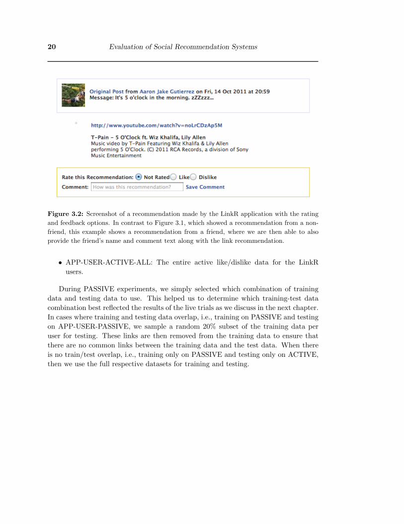
Figure 3.2: Screenshot of a recommendation made by the LinkR application with the rating
and feedback options. In contrast to Figure 3.1, which showed a recommendation from a non-
friend, this example shows a recommendation from a friend, where we are then able to also
provide the friend’s name and comment text along with the link recommendation.
• APP-USER-ACTIVE-ALL: The entire active like/dislike data for the LinkR
users.
During PASSIVE experiments, we simply selected which combination of training
data and testing data to use. This helped us to determine which training-test data
combination best reflected the results of the live trials as we discuss in the next chapter.
In cases where training and testing data overlap, i.e., training on PASSIVE and testing
on APP-USER-PASSIVE, we sample a random 20% subset of the training data per
user for testing. These links are then removed from the training data to ensure that
there are no common links between the training data and the test data. When there
is no train/test overlap, i.e., training only on PASSIVE and testing only on ACTIVE,
then we use the full respective datasets for training and testing.

Chapter 4
Comparison of Existing
Recommender Systems
In this chapter we discuss the first set of four SCF algorithms that was implemented
for the LinkR application and then show how each algorithm performed during the live
user trial, how satisfied the users were with links being recommended to them through
LinkR, and the results of offline passive experiments with the algorithms.
4.1 Objective components
Here we present full derivations for the components of the CF MF methods which we
first described in Section 2.4.2. For the SCF method we use here, we extend the Social
regularization technique also described in Section 2.4.2 to exploit user features as in
Matchbox.
We take a composable approach to collaborative filtering (CF) systems where a
(social) CF minimization objective Obj is composed of sums of one or more objective
components:
Obj =∑i
λiObj i (4.1)
Because each objective may be weighted differently, a weighting term λi ∈ R is included
for each component and should be optimized via cross-validation.
Most target predictions are binary classification-based ({0, 1}), therefore in the
objectives a sigmoidal transform
σ(o) =1
1 + e−o(4.2)
of regressor outputs o ∈ R is used to squash it to the range [0, 1]. In places where the
σ transform may be optionally included, this is written as [σ].
21
22 Comparison of Existing Recommender Systems
4.1.1 Matchbox Matrix Factorization (Obj pmcf )
The basic objective function we use for our MF models is the Matchbox [Stern et al.
2009] model. Matchbox extends the matrix factorization model [Salakhutdinov and
Mnih 2008] for CF by using the user features and item features in learning the latent
spaces for these users and items. The Matchbox MF objective component is:
∑(x,y)∈D
1
2(Rx,y − [σ]xTUTV y)2 (4.3)
4.1.2 L2 U Regularization (Obj ru)
To help in generalization, it is important to regularize the free parameters U and V
to prevent overfitting in the presence of sparse data. This can be done with the L2
regularizer that models a prior of 0 on the parameters. The regularization component
for U is
1
2‖U‖2Fro =
1
2tr(UTU) (4.4)
4.1.3 L2 V Regularization (Obj rv)
We also regularize V as done with U above. The regularization component for V is
1
2‖V ‖2Fro =
1
2tr(V TV ) (4.5)
4.1.4 Social Regularization (Obj rs)
The social aspect of SCF is implemented as a regularizer on the user matrix U . What
this objective component does is constrain users with a high similarity rating to have
the same values in the latent feature space. This models the assumption that users
who are similar socially should also have similar preferences for items.
This method is an extension of existing SCF techniques [Yang et al. 2011; Cui et al.
2011] described in Section 2.4.2 that constrain the latent space to enforce users to have
similar preferences latent representations when they interact heavily. Like Matchbox
which extends regular matrix factorization methods by making use of user and link
features, our extension to the Social Regularization method incorporates user features
to learn similarities between users in the latent space.
§4.1 Objective components 23
∑x
∑z∈friends(x)
1
2(Sx,z − 〈Ux, Uz〉)2
=∑x
∑z∈friends(x)
1
2(Sx,z − xTUTUz)2 (4.6)
4.1.5 Derivatives
We seek to optimize sums of the above objectives and will use gradient descent for this
purpose.
For the overall objective, the partial derivative w.r.t. parameters a are as follows:
∂
∂aObj =
∂
∂a
∑i
λiObj i
=∑i
λi∂
∂aObj i
Previously we noted that that we may want to transform some of the regressor
outputs o[·] using σ(o[·]). This is convenient for our partial derivatives as
∂
∂aσ(o[·]) = σ(o[·])(1− σ(o[·])) ∂
∂ao[·]. (4.7)
Hence anytime a [σ(o[·])] is optionally introduced in place of o[·], we simply insert
[σ(o[·])(1− σ(o[·]))] in the corresponding derivatives below.1
Before we proceed to our objective gradients, we define abbreviations for two useful
vectors:
s = Ux sk = (Ux)k; k = 1 . . .K
t = V y tk = (V y)k; k = 1 . . .K
Please see The Matrix Cookbook [Petersen and Pedersen 2008] for more details on
the matrix derivative identities used in the following calculations.
Now we proceed to derivatives for the previously defined primary objective compo-
nents:
• Matchbox Matrix Factorization: Here we define alternating partial deriva-
tives between U and V , holding one constant and taking the derivative w.r.t. the
1We note that our experiments using the sigmoidal transform in objectives with [0, 1] predictionsdo not generally demonstrate a clear advantage vs. the omission of this transform as originally written(although they do not demonstrate a clear disadvantage either).
24 Comparison of Existing Recommender Systems
other:2
∂
∂UObj pmcf =
∂
∂U
∑(x,y)∈D
1
2
(Rx,y − [σ]
ox,y︷ ︸︸ ︷xTUTV y)︸ ︷︷ ︸
δx,y
2
=∑
(x,y)∈D
δx,y∂
∂U− [σ]xTUT t
= −∑
(x,y)∈D
δx,y[σ(ox,y)(1− σ(ox,y))]txT
∂
∂VObj pmcf =
∂
∂V
∑(x,y)∈D
1
2
(Rx,y − [σ]
ox,y︷ ︸︸ ︷xTUTV y)︸ ︷︷ ︸
δx,y
2
=∑
(x,y)∈D
δx,y∂
∂V− [σ]sTV y
= −∑
(x,y)∈D
δx,y[σ(ox,y)(1− σ(ox,y))]syT
For the regularization objective components, the derivatives are:
• L2 U regularization:
∂
∂UObj ru =
∂
∂U
1
2tr(UTU)
= U
• L2 V regularization:
∂
∂VObj rv =
∂
∂V
1
2tr(V TV )
= V
• Social regularization:
∂
∂UObj rs =
∂
∂U
∑x
∑z∈friends(x)
1
2
Sx,z − xTUTUz︸ ︷︷ ︸δx,y
2
=∑x
∑z∈friends(x)
δx,y∂
∂U− xTUTUz
= −∑x
∑z∈friends(x)
δx,yU(xzT + zxT )
2We will use this method of alternation for all objective components that involve bilinear terms.

§4.2 Algorithms 25
Algorithm Users
Social Matchbox 26Matchbox 26SVM 28Nearest Neighbor 28
Table 4.1: Number of Users Assigned per Algorithm.
Hence, for any choice of primary objective and one or more regularizers, we simply
add the derivatives for U and/or V according to (4.7).
4.2 Algorithms
The CF and SCF algorithms used for the first user trial were:
1. k-Nearest Neighbor (KNN): We use the user-based approach as described in
Section 2.4.1.
2. Support Vector Machines (SVM): We use the the SVM implementation
described in Section 2.3.1 using the features described in Section 3.2.
3. Matchbox (Mbox): Matchbox MF + L2 U Regularization + L2 V Regular-
ization
4. Social Matchbox (Soc. Mbox): Matchbox MF + Social Regularization + L2
Regularization
Social Matchbox uses the Social Regularization method to incorporate the social in-
formation of the FB data. SVM incorporates social information in the fx,y features that
it uses. Matchbox and Nearest Neighbors do not make use of any social information.
4.3 Online Results
The first live user trial was run from August 25 to October 13. The algorithms were
randomly distributed among the 106 users who installed the LinkR application. The
distribution of the algorithms to the users are show in Table 4.1
Each user was recommended three links everyday and they were able to rate the
links on whether they ‘Liked’ or ‘Disliked’ it. Results shown in Figure 4.1 are the
percentage of Like ratings and the percentage of Dislike ratings per algorithm stacked
on top of each other with the Like ratings on top.
As shown in Figure 4.1, Social Matchbox was the best performing algorithm in the
first trial and in fact was the only algorithm to get receive more like ratings than dislike
ratings. This would suggest that using social information does indeed provide useful
information that resulted in better link recommendations from LinkR.
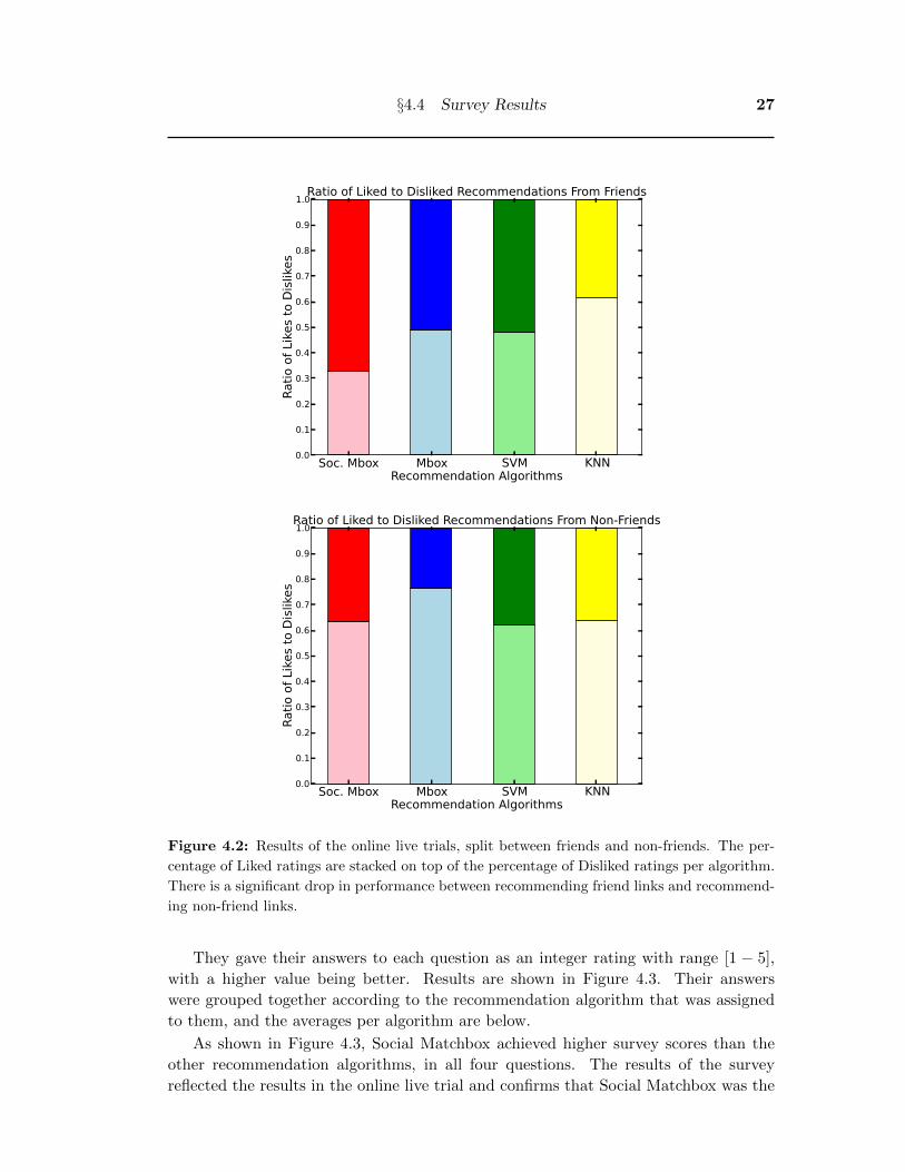
We also look at the algorithms with the results split between friend links and non-
friend links recommendations. Again, the results shown in Figure 4.2 are the percentage
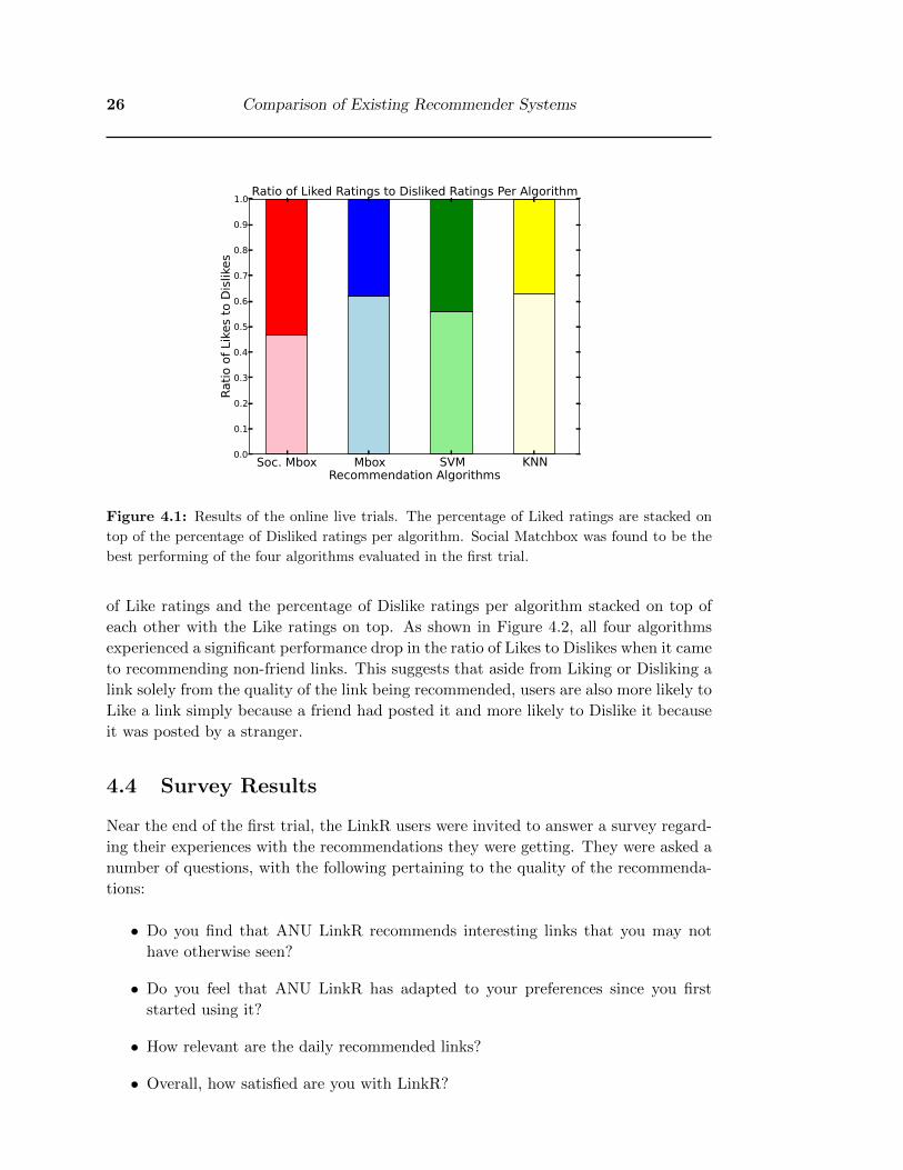
26 Comparison of Existing Recommender Systems
Soc. Mbox Mbox SVM KNNRecommendation Algorithms
0.0
0.1
0.2
0.3
0.4
0.5
0.6
0.7
0.8
0.9
1.0
Ra
tio
of
Like
s to
Dis
like
s
Ratio of Liked Ratings to Disliked Ratings Per Algorithm
Figure 4.1: Results of the online live trials. The percentage of Liked ratings are stacked on
top of the percentage of Disliked ratings per algorithm. Social Matchbox was found to be the
best performing of the four algorithms evaluated in the first trial.
of Like ratings and the percentage of Dislike ratings per algorithm stacked on top of
each other with the Like ratings on top. As shown in Figure 4.2, all four algorithms
experienced a significant performance drop in the ratio of Likes to Dislikes when it came
to recommending non-friend links. This suggests that aside from Liking or Disliking a
link solely from the quality of the link being recommended, users are also more likely to
Like a link simply because a friend had posted it and more likely to Dislike it because
it was posted by a stranger.
4.4 Survey Results
Near the end of the first trial, the LinkR users were invited to answer a survey regard-
ing their experiences with the recommendations they were getting. They were asked a
number of questions, with the following pertaining to the quality of the recommenda-
tions:
• Do you find that ANU LinkR recommends interesting links that you may not
have otherwise seen?
• Do you feel that ANU LinkR has adapted to your preferences since you first
started using it?
• How relevant are the daily recommended links?
• Overall, how satisfied are you with LinkR?
§4.4 Survey Results 27
Soc. Mbox Mbox SVM KNNRecommendation Algorithms
0.0
0.1
0.2
0.3
0.4
0.5
0.6
0.7
0.8
0.9
1.0
Ra
tio
of
Like
s to
Dis
like
s
Ratio of Liked to Disliked Recommendations From Friends
Soc. Mbox Mbox SVM KNNRecommendation Algorithms
0.0
0.1
0.2
0.3
0.4
0.5
0.6
0.7
0.8
0.9
1.0
Ratio of Likes to Dislikes
Ratio of Liked to Disliked Recommendations From Non-Friends
Figure 4.2: Results of the online live trials, split between friends and non-friends. The per-
centage of Liked ratings are stacked on top of the percentage of Disliked ratings per algorithm.
There is a significant drop in performance between recommending friend links and recommend-
ing non-friend links.
They gave their answers to each question as an integer rating with range [1 − 5],
with a higher value being better. Results are shown in Figure 4.3. Their answers
were grouped together according to the recommendation algorithm that was assigned
to them, and the averages per algorithm are below.
As shown in Figure 4.3, Social Matchbox achieved higher survey scores than the
other recommendation algorithms, in all four questions. The results of the survey
reflected the results in the online live trial and confirms that Social Matchbox was the
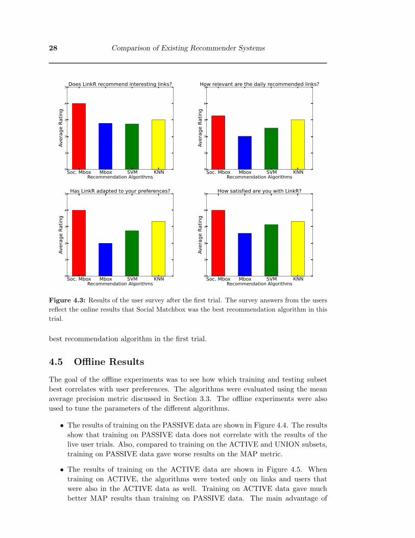
28 Comparison of Existing Recommender Systems
Soc. Mbox Mbox SVM KNNRecommendation Algorithms
0
1
2
3
4
5
Average Rating
Does LinkR recommend interesting links?
Soc. Mbox Mbox SVM KNNRecommendation Algorithms
0
1
2
3
4
5
Avera
ge R
ating
How relevant are the daily recommended links?
Soc. Mbox Mbox SVM KNNRecommendation Algorithms
0
1
2
3
4
5
Average Rating
Has LinkR adapted to your preferences?
Soc. Mbox Mbox SVM KNNRecommendation Algorithms
0
1
2
3
4
5
Avera
ge R
ating
How satisfied are you with LinkR?
Figure 4.3: Results of the user survey after the first trial. The survey answers from the users
reflect the online results that Social Matchbox was the best recommendation algorithm in this
trial.
best recommendation algorithm in the first trial.
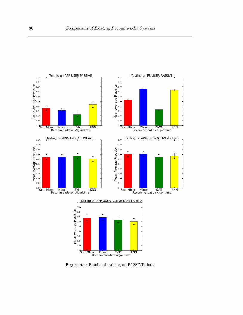
4.5 Offline Results
The goal of the offline experiments was to see how which training and testing subset
best correlates with user preferences. The algorithms were evaluated using the mean
average precision metric discussed in Section 3.3. The offline experiments were also
used to tune the parameters of the different algorithms.
• The results of training on the PASSIVE data are shown in Figure 4.4. The results
show that training on PASSIVE data does not correlate with the results of the
live user trials. Also, compared to training on the ACTIVE and UNION subsets,
training on PASSIVE data gave worse results on the MAP metric.
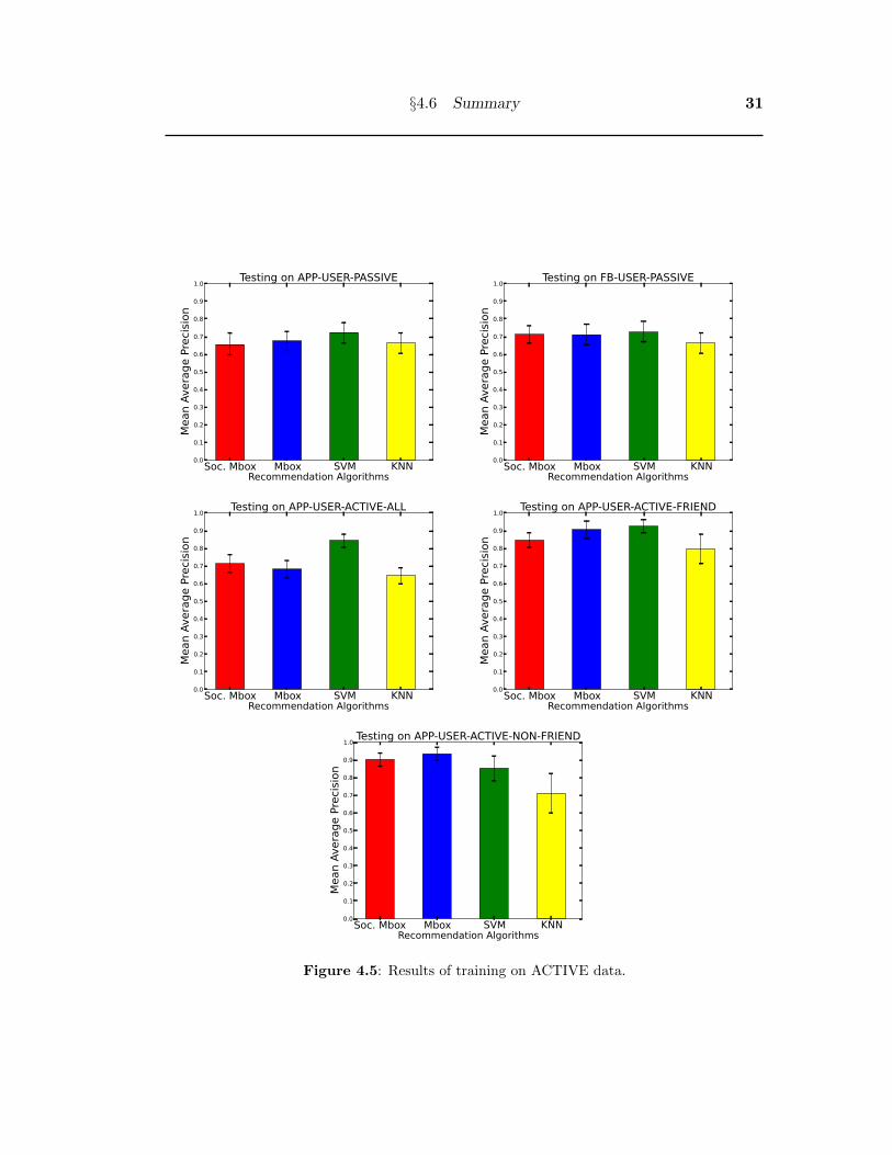
• The results of training on the ACTIVE data are shown in Figure 4.5. When
training on ACTIVE, the algorithms were tested only on links and users that
were also in the ACTIVE data as well. Training on ACTIVE data gave much
better MAP results than training on PASSIVE data. The main advantage of

§4.6 Summary 29
ACTIVE data over PASSIVE data is the explicit dislikes that only the ACTIVE
data has. Even though the ACTIVE data is far smaller than the PASSIVE data,
this inclusion of explicit dislikes allowed the SCF algorithms to perform better in
the offline experiments.
However, one weakness of ACTIVE is the small amount of data in it, only the
explicit likes and dislikes of only the LinkR application users. ACTIVE data can’t
provide information on LinkR users that have just installed the application, old
LinkR users that haven’t rated any links, and other non-LinkR users on Facebook.
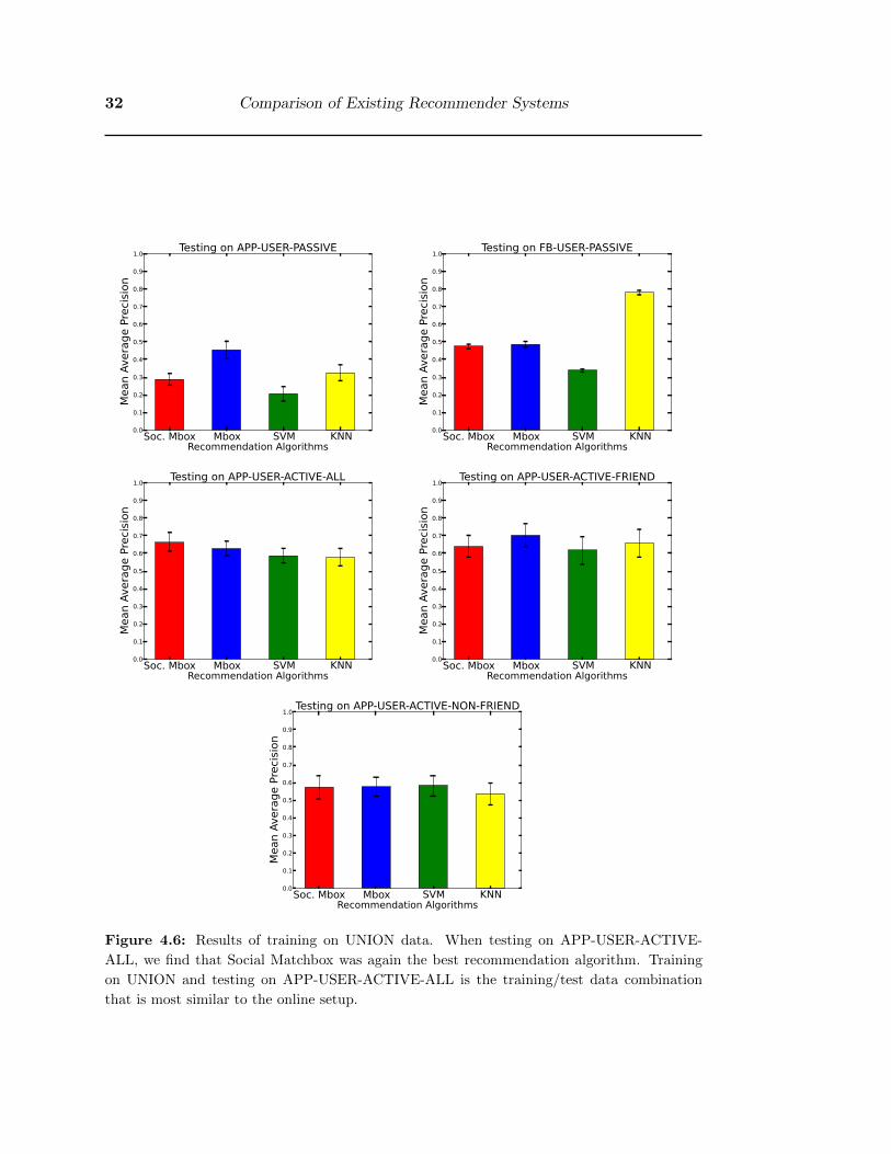
• The results of training on UNION data are shown in Figure 4.6. UNION combines
the advantage of PASSIVE with having a larger dataset and the advantage of
ACTIVE. When testing on the APP-USER-ACTIVE-ALL dataset, the results
correlate with the results of the live user trial and the user surveys.
To give the best recommendations for all users, the SCF algorithms are best trained
on the larger size of the PASSIVE data with the explicit likes and dislikes of the AC-
TIVE data. Hence, for the second user trial in the next chapter we keep on training
the UNION dataset.
4.6 Summary
At the end of the first trial, we have observed the following:
• Social Matchbox was the best performing algorithm in the live user trial in terms
of percentage of likes.
• Social Matchbox received the highest user evaluation scores in the user survey at
the end of the user trial.
• Of the various combinations of training and testing data in the offline passive
experiment, we found that training on the UNION subset and testing on the APP-
USER-ACTIVE-ALL subset best correlated with the results of the live user trial
and the user survey. Training on the UNION dataset had advantages compared
to training on the other data subsets, namely that it had the large amount of
information of the PASSIVE data and the explicit dislikes information of the
ACTIVE data.
In the next chapter, we discuss new techniques for incorporating social information
and show how they improve on Social Matchbox.
30 Comparison of Existing Recommender Systems
Soc. Mbox Mbox SVM KNNRecommendation Algorithms
0.0
0.1
0.2
0.3
0.4
0.5
0.6
0.7
0.8
0.9
1.0
Me
an
Av
era
ge
Pre
cisi
on
Testing on APP-USER-PASSIVE
Soc. Mbox Mbox SVM KNNRecommendation Algorithms
0.0
0.1
0.2
0.3
0.4
0.5
0.6
0.7
0.8
0.9
1.0
Mean Average Precision
Testing on FB-USER-PASSIVE
Soc. Mbox Mbox SVM KNNRecommendation Algorithms
0.0
0.1
0.2
0.3
0.4
0.5
0.6
0.7
0.8
0.9
1.0
Mean Average Precision
Testing on APP-USER-ACTIVE-ALL
Soc. Mbox Mbox SVM KNNRecommendation Algorithms
0.0
0.1
0.2
0.3
0.4
0.5
0.6
0.7
0.8
0.9
1.0
Mean Average Precision
Testing on APP-USER-ACTIVE-FRIEND
Soc. Mbox Mbox SVM KNNRecommendation Algorithms
0.0
0.1
0.2
0.3
0.4
0.5
0.6
0.7
0.8
0.9
1.0
Mean Average Precision
Testing on APP-USER-ACTIVE-NON-FRIEND
Figure 4.4: Results of training on PASSIVE data.
§4.6 Summary 31
Soc. Mbox Mbox SVM KNNRecommendation Algorithms
0.0
0.1
0.2
0.3
0.4
0.5
0.6
0.7
0.8
0.9
1.0
Me
an
Av
era
ge
Pre
cisi
on
Testing on APP-USER-PASSIVE
Soc. Mbox Mbox SVM KNNRecommendation Algorithms
0.0
0.1
0.2
0.3
0.4
0.5
0.6
0.7
0.8
0.9
1.0
Mean Average Precision
Testing on FB-USER-PASSIVE
Soc. Mbox Mbox SVM KNNRecommendation Algorithms
0.0
0.1
0.2
0.3
0.4
0.5
0.6
0.7
0.8
0.9
1.0
Mean Average Precision
Testing on APP-USER-ACTIVE-ALL
Soc. Mbox Mbox SVM KNNRecommendation Algorithms
0.0
0.1
0.2
0.3
0.4
0.5
0.6
0.7
0.8
0.9
1.0
Mean Average Precision
Testing on APP-USER-ACTIVE-FRIEND
Soc. Mbox Mbox SVM KNNRecommendation Algorithms
0.0
0.1
0.2
0.3
0.4
0.5
0.6
0.7
0.8
0.9
1.0
Mean Average Precision
Testing on APP-USER-ACTIVE-NON-FRIEND
Figure 4.5: Results of training on ACTIVE data.
32 Comparison of Existing Recommender Systems
Soc. Mbox Mbox SVM KNNRecommendation Algorithms
0.0
0.1
0.2
0.3
0.4
0.5
0.6
0.7
0.8
0.9
1.0
Me
an
Av
era
ge
Pre
cisi
on
Testing on APP-USER-PASSIVE
Soc. Mbox Mbox SVM KNNRecommendation Algorithms
0.0
0.1
0.2
0.3
0.4
0.5
0.6
0.7
0.8
0.9
1.0
Mean Average Precision
Testing on FB-USER-PASSIVE
Soc. Mbox Mbox SVM KNNRecommendation Algorithms
0.0
0.1
0.2
0.3
0.4
0.5
0.6
0.7
0.8
0.9
1.0
Mean Average Precision
Testing on APP-USER-ACTIVE-ALL
Soc. Mbox Mbox SVM KNNRecommendation Algorithms
0.0
0.1
0.2
0.3
0.4
0.5
0.6
0.7
0.8
0.9
1.0
Mean Average Precision
Testing on APP-USER-ACTIVE-FRIEND
Soc. Mbox Mbox SVM KNNRecommendation Algorithms
0.0
0.1
0.2
0.3
0.4
0.5
0.6
0.7
0.8
0.9
1.0
Mean Average Precision
Testing on APP-USER-ACTIVE-NON-FRIEND
Figure 4.6: Results of training on UNION data. When testing on APP-USER-ACTIVE-
ALL, we find that Social Matchbox was again the best recommendation algorithm. Training
on UNION and testing on APP-USER-ACTIVE-ALL is the training/test data combination
that is most similar to the online setup.
Chapter 5
New Algorithms for Social
Recommendation
After studying the results of the first trial, we made use of what we learned to design
new algorithms to improve upon deficiencies of existing recommendation algorithms.
Our goal in designing these algorithms was to address deficiencies in current SCF
methods that was previously discussed at-length in Section 1.1:
• Non-feature-based user similarity
• Modeling direct user-user information diffusion
• Restricted common interests
We address these deficiencies by modifying the optimization objectives that were
discussed in the previous chapter, creating new objective functions. We discuss these
new objectives in the following sections.
5.1 New Objective Components
As in Chapter 4, we assume that the CF optimization objective decomposes into a sum
of objective components as follows:
Obj =∑i
λiObj i (5.1)
5.1.1 Hybrid Objective (Obj phy )
As specified in Chapter 1, one weakness of MF methods is that they cannot model joint
features over user and items, and hence the cannot model direct user-user information
diffusion. Information diffusion models the unidirectional flow of links from one user
to another (i.e., one user likes/shares what another user posts). We believe that this
information will be useful for SCF, and is lacking in current SCF methods.
33
34 New Algorithms for Social Recommendation
We fix this by introducing another objective component in addition to the standard
MF objective, and this component serves as a simple linear regressor for such infor-
mation diffusion observations. The resulting hybrid objective component becomes a
combination of latent MF and linear regression objectives.
We make use of the fx,y features detailed in Section 3.2 to make the linear regressor.
fx,y models user-user information diffusion because it is a joint feature between users
and the links. It allows us to learn information diffusion models whether certain users
always likes content from another specific user.
Using 〈·, ·〉 to denote an inner product, we define a weight vector w ∈ RF such
that 〈w, fx,y〉 = wT fx,y is the prediction of the system. The objective of the linear
regression component is therefore
∑(x,y)∈D
1
2(Rx,y − [σ]wT fx,y)2
We combine the output of the linear regression objective with the Matchbox output
[σ]xTUTV y, to get a hybrid objective component. The full objective function for this
hybrid model is
∑(x,y)∈D
1
2(Rx,y − [σ]wT fx,y − [σ]xTUTV y)2 (5.2)
5.1.2 L2 w Regularization (Obj rw)
In the same manner as U and V , it is important to regularize the free parameter w to
prevent overfitting in the presence of sparse data. This can again be done with the L2
regularizer that models a prior of 0 on the parameters. The objective component for
the L2 regularizer for w is:
1
2‖w‖22 =
1
2wTw (5.3)
5.1.3 Social Spectral Regularization (Obj rss)
As we did with the Social Regularization method in Section 4.1.4, we build on ideas used
in Matchbox [Stern et al. 2009] to extend social spectral regularization [Ma et al. 2011;
Li and Yeung 2009] by incorporating user features into the objective. The objective
function for our extension to social spectral regularization is:
§5.1 New Objective Components 35
∑x
∑z∈friends(x)
1
2S+x,z‖Ux− Uz‖22
=∑x
∑z∈friends(x)
1
2S+x,z‖U(x− z)‖22
=∑x
∑z∈friends(x)
1
2S+x,z(x− z)TUTU(x− z) (5.4)
5.1.4 Social Co-preference Regularization (Obj rsc)
A crucial aspect missing from other SCF methods is that while two users may not
be globally similar or opposite in their preferences, there may be sub-areas of their
interests which can be correlated to each other. For example, two friends may have
similar interests concerning music, but different interests concerning politics. The social
co-preference regularizers aim to learn such selective co-preferences. The motivation is
to constrain users x and z who have similar or opposing preferences to be similar or
opposite in the same latent latent space relevant to item y.
We use 〈·, ·〉• to denote a re-weighted inner product. The purpose of this inner
product is to tailor the latent space similarities or dissimilarities between users to
specific sets of items. This fixes the issue detailed in the previous paragraph by allowing
users x and z to be similar or opposite in the same latent latent space relevant only to
item y.
The objective component for social co-preference regularization along with its ex-
panded form is
∑(x,z,y)∈C
1
2(Px,z,y − 〈Ux, Uz〉V y)2
=∑
(x,z,y)∈C
1
2(Px,z,y − xTUT diag(V y)Uz)2 (5.5)
5.1.5 Social Co-preference Spectral Regularization (Obj rscs)
This is the same as the social co-preference regularization above, except that it uses
the spectral regularizer format for learning the co-preferences.
We use ‖ · ‖2,• to denote a re-weighted L2 norm. The reweighing of this norm
servers the same purpose as the re-weighted inner product in Section 5.1.4, it tailors
the similarities or dissimilarities between users to specific sets of items. This allows
users x and z to be similar or opposite in the same latent latent space relevant only to
item y.
The objective component for social co-preference spectral regularization along with
its expanded form is
36 New Algorithms for Social Recommendation
∑(x,z,y)∈C
1
2Px,z,y‖Ux− Uz‖22,V y
=∑
(x,z,y)∈C
1
2Px,z,y‖U(x− z)‖22,V y
=∑
(x,z,y)∈C
1
2Px,z,y(x− z)TUT diag(V y)U(x− z) (5.6)
5.1.6 Derivatives
As before, we seek to optimize sums of the above objectives and will use gradient descent
for this purpose. Please see The Matrix Cookbook [Petersen and Pedersen 2008] for
more details on the matrix derivative identities used in the following calculations. We
again use the following useful abbreviations:
s = Ux sk = (Ux)k; k = 1 . . .K
t = V y tk = (V y)k; k = 1 . . .K
The derivatives for the hybrid objective functions as well as the new social regular-
izers are:
• Hybrid:
∂
∂wObj phy =
∂
∂w
∑(x,y)∈D
1
2
Rx,y − [σ]
o1x,y︷ ︸︸ ︷wT fx,y−[σ]xTUTV y︸ ︷︷ ︸
δx,y
2
=∑
(x,y)∈D
δx,y∂
∂w− [σ]wT fx,y
= −∑
(x,y)∈D
δx,y[σ(o1x,y)(1− σ(o1x,y))]fx,y
§5.1 New Objective Components 37
∂
∂UObj phy =
∂
∂U
∑(x,y)∈D
1
2
Rx,y − [σ]wT fx,y − [σ]
o2x,y︷ ︸︸ ︷xTUTV y︸ ︷︷ ︸
δx,y
2
=∑
(x,y)∈D
δx,y∂
∂U− [σ]xTUTV y
= −∑
(x,y)∈D
δx,y[σ(o2x,y)(1− σ(o2x,y))]txT
∂
∂VObj phy =
∂
∂V
∑(x,y)∈D
1
2
Rx,y − [σ]wT fx,y − [σ]
o2x,y︷ ︸︸ ︷xTUTV y︸ ︷︷ ︸
δx,y
2
=∑
(x,y)∈D
δx,y∂
∂V− [σ]xTUTV y
= −∑
(x,y)∈D
δx,y[σ(o2x,y)(1− σ(o2x,y))]syT
• L2 w regularization:
∂
∂wObj rw =
∂
∂w
1
2wTw
= w
• Social spectral regularization:
∂
∂UObj rss =
∂
∂U
∑x
∑z∈friends(x)
1
2S+x,z(x− z)TUTU(x− z)
=∑x
∑z∈friends(x)
1
2S+x,zU((x− z)(x− z)T + (x− z)(x− z)T )
=∑x
∑z∈friends(x)
S+x,zU(x− z)(x− z)T
Before we proceed to the final derivatives, we define one additional vector abbreviation:
r = Uz rk = (Uz)k; k = 1 . . .K.
38 New Algorithms for Social Recommendation
• Social co-preference regularization:
∂
∂UObj rsc =
∂
∂U
∑(x,z,y)∈C
1
2
Px,z,y − xTUT diag(V y)Uz︸ ︷︷ ︸δx,z,y
2
=∑
(x,z,y)∈C
δx,z,y∂
∂U− xTUT diag(V y)Uz
= −∑
(x,z,y)∈C
δx,z,y(diag(V y)TUxzT + diag(V y)UzxT )
= −∑
(x,z,y)∈C
δx,z,y diag(V y)U(xzT + zxT )
In the following, ◦ is the Hadamard elementwise product:
∂
∂VObj rsc =
∂
∂V
∑(x,z,y)∈C
1
2(Px,z,y − xTUT diag(V y)Uz)2
=∂
∂V
∑(x,z,y)∈C
1
2
Px,z,y − (
s︷︸︸︷Ux ◦
r︷︸︸︷Uz )TV y︸ ︷︷ ︸
δx,z,y
2
=∑
(x,z,y)∈C
δx,z,y∂
∂V− (s ◦ r)TV y
= −∑
(x,z,y)∈C
δx,z,y(s ◦ r)yT
§5.2 Second Trial 39
• Social co-preference spectral regularization:
∂
∂UObj rscs =
∂
∂U
∑(x,z,y)∈C
1
2Px,z,y(x− z)TUT diag(V y)U(x− z)
=∑
(x,z,y)∈C
1
2Px,z,y
(diag(V y)TU(x− z)(x− z)T
+ diag(V y)U(x− z)(x− z)T)
=∑
(x,z,y)∈C
Px,z,y diag(V y)U(x− z)(x− z)T
∂
∂VObj rscs =
∂
∂V
∑(x,z,y)∈C
1
2Px,z,y(x− z)TUT diag(V y)U(x− z)
=∂
∂V
∑(x,z,y)∈C
1
2Px,z,y(U(x− z) ◦ U(x− z))TV y
=1
2
∑(x,z,y)∈C
Px,z,y(U(x− z) ◦ U(x− z))yT
Hence, for any choice of primary objective and one or more regularizers, we simply
add the derivatives for each of w, U , and V according to (4.7).
5.2 Second Trial
For the second online trial, we chose four algorithms again to randomly split between
the LinkR application users. Social Matchbox was included again as a baseline since
it was the best performing algorithm in the first trial. The distribution count of the
algorithms to the users is shown in Table 5.1
The four SCF algorithms are:
• Social Matchbox (Soc. Mbox) : Matchbox MF + Social Regularization +
L2 U Regularization + L2 V Regularization
• Spectral Matchbox (Spec. Mbox): Matchbox MF + Social Spectral Regu-
larization + L2 U Regularization + L2 V Regularization
• Social Hybrid (Soc. Hybrid): Hybrid + Social Regularization + L2 U Reg-
ularization + L2 V Regularization + L2 w Regularization
• Spectral Co-preference (Spec. CP): Matchbox MF + Social Co-preference
Spectral Regularization + L2 U Regularization + L2 V Regularization
5.2.1 Online Results
The online experiments were switched to the new algorithms on October 13, 2011. For
the online results reported here, since the second live trial is still currently ongoing,
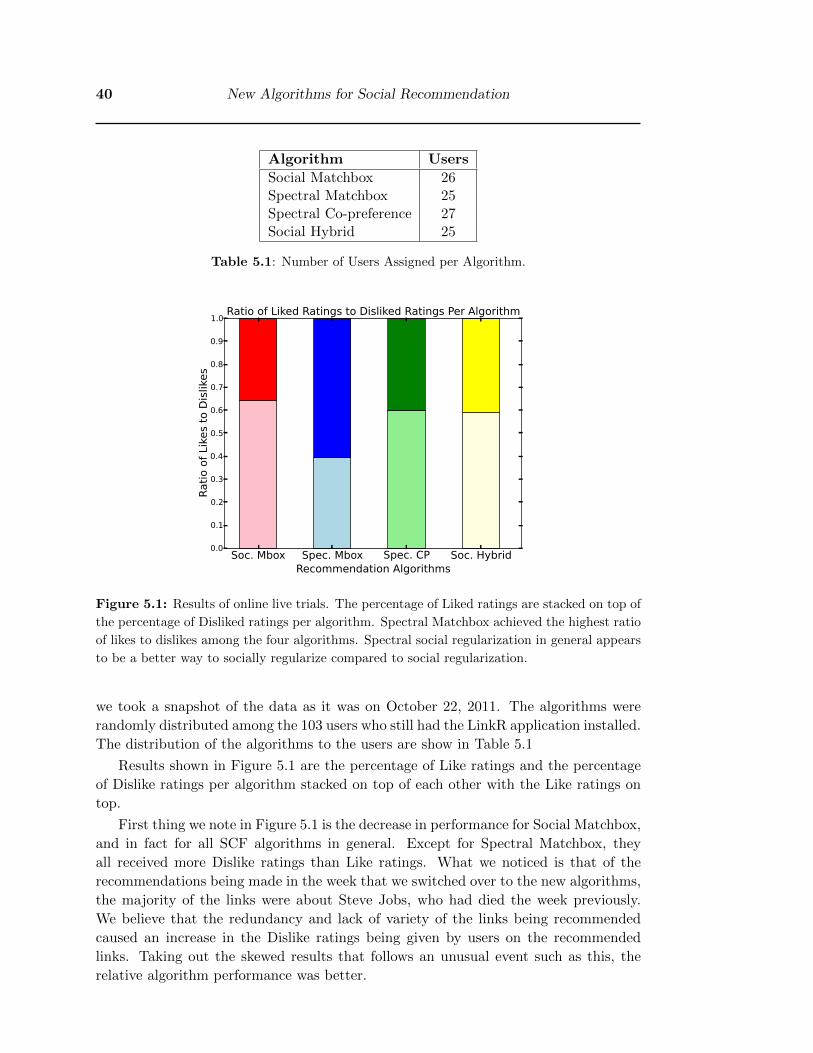
40 New Algorithms for Social Recommendation
Algorithm Users
Social Matchbox 26Spectral Matchbox 25Spectral Co-preference 27Social Hybrid 25
Table 5.1: Number of Users Assigned per Algorithm.
Soc. Mbox Spec. Mbox Spec. CP Soc. HybridRecommendation Algorithms
0.0
0.1
0.2
0.3
0.4
0.5
0.6
0.7
0.8
0.9
1.0
Ratio of Likes to Dislikes
Ratio of Liked Ratings to Disliked Ratings Per Algorithm
Figure 5.1: Results of online live trials. The percentage of Liked ratings are stacked on top of
the percentage of Disliked ratings per algorithm. Spectral Matchbox achieved the highest ratio
of likes to dislikes among the four algorithms. Spectral social regularization in general appears
to be a better way to socially regularize compared to social regularization.
we took a snapshot of the data as it was on October 22, 2011. The algorithms were
randomly distributed among the 103 users who still had the LinkR application installed.
The distribution of the algorithms to the users are show in Table 5.1
Results shown in Figure 5.1 are the percentage of Like ratings and the percentage
of Dislike ratings per algorithm stacked on top of each other with the Like ratings on
top.
First thing we note in Figure 5.1 is the decrease in performance for Social Matchbox,
and in fact for all SCF algorithms in general. Except for Spectral Matchbox, they
all received more Dislike ratings than Like ratings. What we noticed is that of the
recommendations being made in the week that we switched over to the new algorithms,
the majority of the links were about Steve Jobs, who had died the week previously.
We believe that the redundancy and lack of variety of the links being recommended
caused an increase in the Dislike ratings being given by users on the recommended
links. Taking out the skewed results that follows an unusual event such as this, the
relative algorithm performance was better.
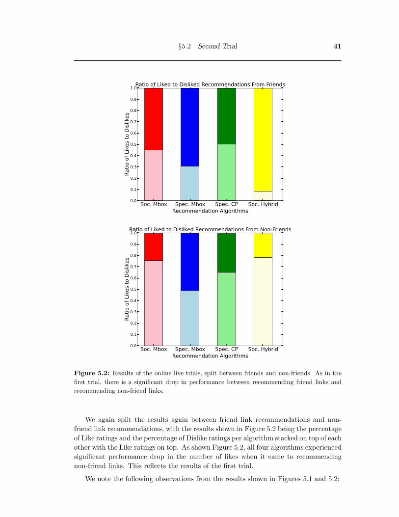
§5.2 Second Trial 41
Soc. Mbox Spec. Mbox Spec. CP Soc. HybridRecommendation Algorithms
0.0
0.1
0.2
0.3
0.4
0.5
0.6
0.7
0.8
0.9
1.0
Ra
tio
of
Like
s to
Dis
like
s
Ratio of Liked to Disliked Recommendations From Friends
Soc. Mbox Spec. Mbox Spec. CP Soc. HybridRecommendation Algorithms
0.0
0.1
0.2
0.3
0.4
0.5
0.6
0.7
0.8
0.9
1.0
Ra
tio
of
Like
s to
Dis
like
s
Ratio of Liked to Disliked Recommendations From Non-Friends
Figure 5.2: Results of the online live trials, split between friends and non-friends. As in the
first trial, there is a significant drop in performance between recommending friend links and
recommending non-friend links.
We again split the results again between friend link recommendations and non-
friend link recommendations, with the results shown in Figure 5.2 being the percentage
of Like ratings and the percentage of Dislike ratings per algorithm stacked on top of each
other with the Like ratings on top. As shown Figure 5.2, all four algorithms experienced
significant performance drop in the number of likes when it came to recommending
non-friend links. This reflects the results of the first trial.
We note the following observations from the results shown in Figures 5.1 and 5.2:
42 New Algorithms for Social Recommendation
• Compared to the other algorithms, Spectral Matchbox achieved the best ratio
of likes to dislikes as seen, as seen in Figure 5.1. Combined with the results for
Spectral Co-preference, Spectral social regularization in general appears to be a
better way to socially regularize compared to social regularization. This compar-
ison holds even when the results are split between friend links recommendations
and non-friend links recommendations, as seen in Figure 5.2.
• When looking at just the friend link recommendations in Figure 5.2, Social Hy-
brid was the best performing algorithm. This result comes from the user-user
information diffusion among its friends that Social Hybrid learns, which could
not be learned by the other SCF algorithms. Learning information diffusion thus
helps when it comes to building better SCF algorithms.
• Spectral Co-preference didn’t do well on friend link recommendations, however
it did better on the non-friend link recommendations. When it comes to recom-
mending friend links, friend interaction information coming through social regu-
larizer seems more important than implicit co-likes information provided by the
co-preference regularizer. When there is no social interaction information such as
with non-friend links, co-preference methods with its implicit co-likes information
appear much better than just vanilla collaborative filtering at projecting users
into subspaces of common interest.
5.3 Offline Results
Aside from the online user trial, we also evaluate the algorithms using the mean average
precision metric discussed in Section 3.3. We note the following observations from the
results shown in Figures 5.3, 5.4, and 5.5:
• Most results are not statistically significant.
• In Figure 5.5, when training UNION and testing on APP-USER-ACTIVE-FRIEND,
Social Hybrid gets the score on the MAP metric. This reflects the results of the
live user trial in Section 5.2.1.
• In Figure 5.4, when training on ACTIVE and testing on APP-USER-ACTIVE-
NON-FRIEND, Spectral Co-preference shows slightly better (though not sta-
tistically significant) performance than when testing on APP-USER-ACTIVE-
FRIEND. This also reflects the results of the live user trial in Section 5.2.1. The
explicit dislikes of the Active data allow the co-preference regularizer to learn the
Dislike data better.
• The better performance of the social spectral regularization methods in the live
user trials do not show in the offline experiments. This may be caused by the dif-
ference in the dataset size between the live user trials and the offline experiments,
which affected optimal parameter settings for the offline experiments. Further
tuning of the parameters may cause the social spectral regularization methods to
perform better
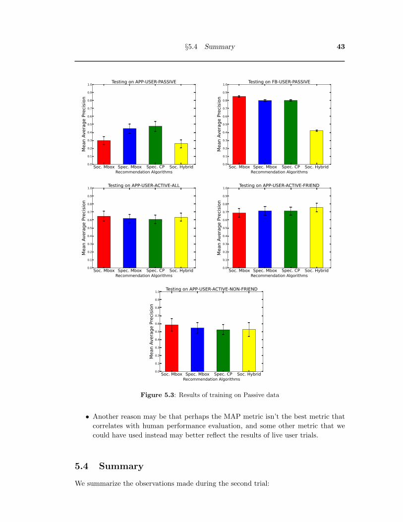
§5.4 Summary 43
Soc. Mbox Spec. Mbox Spec. CP Soc. HybridRecommendation Algorithms
0.0
0.1
0.2
0.3
0.4
0.5
0.6
0.7
0.8
0.9
1.0M
ea
n A
ve
rag
e P
reci
sio
nTesting on APP-USER-PASSIVE
Soc. Mbox Spec. Mbox Spec. CP Soc. HybridRecommendation Algorithms
0.0
0.1
0.2
0.3
0.4
0.5
0.6
0.7
0.8
0.9
1.0
Mean Average Precision
Testing on FB-USER-PASSIVE
Soc. Mbox Spec. Mbox Spec. CP Soc. HybridRecommendation Algorithms
0.0
0.1
0.2
0.3
0.4
0.5
0.6
0.7
0.8
0.9
1.0
Mean Average Precision
Testing on APP-USER-ACTIVE-ALL
Soc. Mbox Spec. Mbox Spec. CP Soc. HybridRecommendation Algorithms
0.0
0.1
0.2
0.3
0.4
0.5
0.6
0.7
0.8
0.9
1.0
Mean Average Precision
Testing on APP-USER-ACTIVE-FRIEND
Soc. Mbox Spec. Mbox Spec. CP Soc. HybridRecommendation Algorithms
0.0
0.1
0.2
0.3
0.4
0.5
0.6
0.7
0.8
0.9
1.0
Mean Average Precision
Testing on APP-USER-ACTIVE-NON-FRIEND
Figure 5.3: Results of training on Passive data
• Another reason may be that perhaps the MAP metric isn’t the best metric that
correlates with human performance evaluation, and some other metric that we
could have used instead may better reflect the results of live user trials.
5.4 Summary
We summarize the observations made during the second trial:
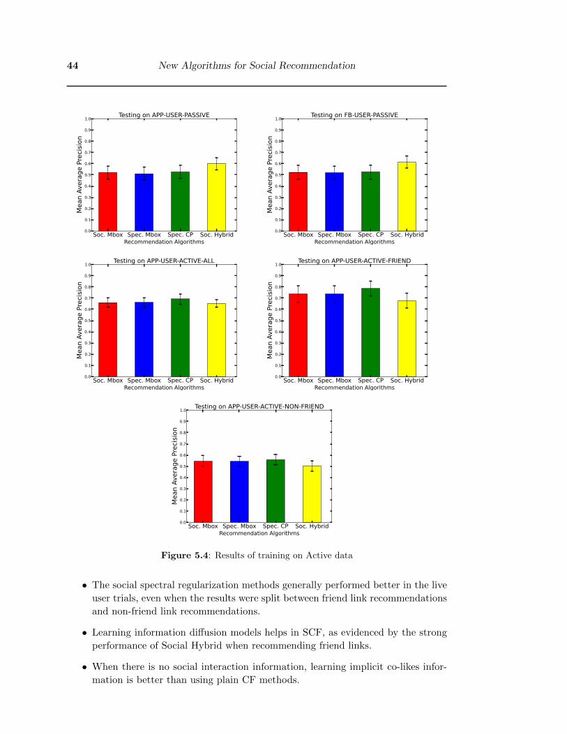
44 New Algorithms for Social Recommendation
Soc. Mbox Spec. Mbox Spec. CP Soc. HybridRecommendation Algorithms
0.0
0.1
0.2
0.3
0.4
0.5
0.6
0.7
0.8
0.9
1.0
Me
an
Av
era
ge
Pre
cisi
on
Testing on APP-USER-PASSIVE
Soc. Mbox Spec. Mbox Spec. CP Soc. HybridRecommendation Algorithms
0.0
0.1
0.2
0.3
0.4
0.5
0.6
0.7
0.8
0.9
1.0
Mean Average Precision
Testing on FB-USER-PASSIVE
Soc. Mbox Spec. Mbox Spec. CP Soc. HybridRecommendation Algorithms
0.0
0.1
0.2
0.3
0.4
0.5
0.6
0.7
0.8
0.9
1.0
Mean Average Precision
Testing on APP-USER-ACTIVE-ALL
Soc. Mbox Spec. Mbox Spec. CP Soc. HybridRecommendation Algorithms
0.0
0.1
0.2
0.3
0.4
0.5
0.6
0.7
0.8
0.9
1.0Mean Average Precision
Testing on APP-USER-ACTIVE-FRIEND
Soc. Mbox Spec. Mbox Spec. CP Soc. HybridRecommendation Algorithms
0.0
0.1
0.2
0.3
0.4
0.5
0.6
0.7
0.8
0.9
1.0
Mean Average Precision
Testing on APP-USER-ACTIVE-NON-FRIEND
Figure 5.4: Results of training on Active data
• The social spectral regularization methods generally performed better in the live
user trials, even when the results were split between friend link recommendations
and non-friend link recommendations.
• Learning information diffusion models helps in SCF, as evidenced by the strong
performance of Social Hybrid when recommending friend links.
• When there is no social interaction information, learning implicit co-likes infor-
mation is better than using plain CF methods.
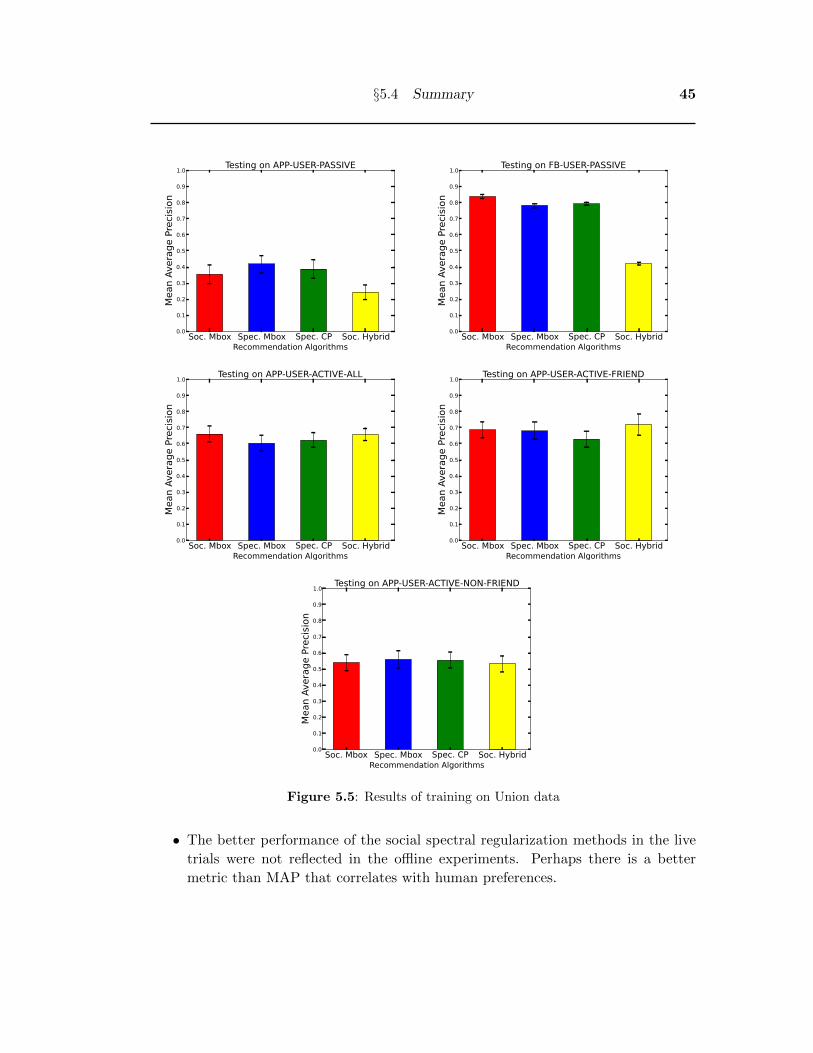
§5.4 Summary 45
Soc. Mbox Spec. Mbox Spec. CP Soc. HybridRecommendation Algorithms
0.0
0.1
0.2
0.3
0.4
0.5
0.6
0.7
0.8
0.9
1.0M
ea
n A
ve
rag
e P
reci
sio
nTesting on APP-USER-PASSIVE
Soc. Mbox Spec. Mbox Spec. CP Soc. HybridRecommendation Algorithms
0.0
0.1
0.2
0.3
0.4
0.5
0.6
0.7
0.8
0.9
1.0
Mean Average Precision
Testing on FB-USER-PASSIVE
Soc. Mbox Spec. Mbox Spec. CP Soc. HybridRecommendation Algorithms
0.0
0.1
0.2
0.3
0.4
0.5
0.6
0.7
0.8
0.9
1.0
Mean Average Precision
Testing on APP-USER-ACTIVE-ALL
Soc. Mbox Spec. Mbox Spec. CP Soc. HybridRecommendation Algorithms
0.0
0.1
0.2
0.3
0.4
0.5
0.6
0.7
0.8
0.9
1.0
Mean Average Precision
Testing on APP-USER-ACTIVE-FRIEND
Soc. Mbox Spec. Mbox Spec. CP Soc. HybridRecommendation Algorithms
0.0
0.1
0.2
0.3
0.4
0.5
0.6
0.7
0.8
0.9
1.0
Mean Average Precision
Testing on APP-USER-ACTIVE-NON-FRIEND
Figure 5.5: Results of training on Union data
• The better performance of the social spectral regularization methods in the live
trials were not reflected in the offline experiments. Perhaps there is a better
metric than MAP that correlates with human preferences.

46 New Algorithms for Social Recommendation
Chapter 6
Conclusion
6.1 Summary
In this thesis, we evaluated existing algorithms and proposed new algorithms for social
collaborative filtering via the task of link recommendation on Facebook.
In Chapter 2, we outlined three main deficiencies in current social collaborative
filtering (SCF) techniques and proposed new techniques in Chapters 4 and 5 to solve
them; we review them here as follows:
(a) Non-feature-based user similarity: We extended existing social regulariza-
tion and social spectral regularization methods to incorporate user features to
learn user-user similarities in the latent space.
(b) Model direct user-user information diffusion: We defined a new hybrid
SCF method where we combined the collaborative filtering (CF) matrix factor-
ization (MF) objective used by Matchbox [Stern et al. 2009] with a linear content-
based filtering (CBF) objective used to model direct user-user information diffu-
sion in the social network.
(c) Restricted common interests: We defined a new social co-preference regular-
ization method that learns from pairs of user preferences over the same item to
learn user similarities in specific areas — a contrast to previous methods that
typically enforce global user similarity when regularizing.
Having evaluated existing baselines (with minor extensions) in Chapter 4 and evalu-
ating these new algorithms in Chapter 5 in live online user trials with over 100 Facebook
App users and data for over 30,000 unique Facebook users, we summarize the main
results of the thesis:
• Our extensions to social regularization in Chapter 4 and Chapter 5 proved to
be very effective methods for SCF, and outperformed all other algorithms in the
first Facebook user evaluation trial. This was reflected in the live user trial, user
survey, and offline passive experimental results. However, our socially regularized
SCF MF extension in Chapter 4 could still be improved by changing to a spectral
approach, and this further extension in Chapter 5 generally outperformed the
47
48 Conclusion
SCF socially regularized extension of Chapter 4. The take-home point is that a
very useful form of social regularization appears to be social spectral regularization
as proposed in Chapter 5.
• Learning direct user-user information diffusion models (i.e., how much one user
likes links posted by another) can result in improved SCF algorithms in compar-
ison to standard MF methods. To this end, our social hybrid algorithm which
uses this information outperformed all other SCF methods when recommending
friend links as shown in Chapter 5.
• Friend interaction information coming from social regularization is more useful
than the implicit co-likes information of co-preference regularization. However,
when there is no social interaction information available (as in the case of recom-
mending non-friend links), learning this implicit co-likes information outperforms
plain CF methods as evidenced by the relative success of the co-preference regu-
larization algorithm as demonstrated in Chapter 5.
• Knowing what offline metrics for measuring SCF performance correlate with hu-
man preferences from live trials is crucial for efficient evaluation of SCF algo-
rithms and also quite useful for offline algorithm tuning. In general, as most
strongly evidenced in Chapter 4, it appears that evaluating mean average preci-
sion (MAP) when training on data that includes both passively inferred dislikes
and explicit negative preference feedback (i.e., explicit dislikes indicated via the
Facebook App), but evaluating MAP only with explicit feedback (no inferred
dislikes) seems to be a train/test evaluation approach and evaluation metric that
correlates with human survey feedback.
Hence, this thesis has made a number of substantial contributions to SCF recom-
mendation systems and has helped advance methods for SCF system evaluation.
6.2 Future Work
This work just represents the tip of the iceberg in different improvements that SCF can
make over more traditional non-social CF methods. Here we identify a number of addi-
tional future extensions that can potentially further improve the proposed algorithms
in this thesis:
• We used only a subset of the possible feature data in Facebook and in the links
themselves. Extending the social recommenders to handle more of the rich infor-
mation that is available may result in better performance for the SCF algorithms.
One critical feature that would have been useful is including a genre feature in the
links (e.g., indicating whether the link represented a blog, news, video, etc.) to
provide a fine-grained model of which types of links that users prefers to receive.
This additional information would have likely prevented a number of observed
dislikes from users regarding specific genres of links, e.g., those that do not listen
§6.2 Future Work 49
to music much and hence do not care about links to music videos — even if these
links are otherwise liked by friends and very popular.
• Enforcing diversity in the recommended links would prevent redundant links
about the same topic being recommended again and again. This is especially
useful when an unusual event happens like the death of Steve Jobs and the en-
suing massive amount of Steve Jobs related links that flooded Facebook. While
users may like to see a few links on the topic, their interest in similar links
decreases over time and diversity in recommendations could help address this
saturation effect.
• Another future direction this work can go to is to incorporate active learning in
the algorithms. This would ensure that the SCF algorithm did not exploit the
learned preferences too much and made an active effort to discover better link
preferences that are available.
• Probably the biggest assumption we have made in our implementations is how
we inferred the implicit dislikes of users in the Facebook data. A better and
method of inferring implicit dislikes will give a big boost to the SCF algorithms.
As evidenced by the results of training on ACTIVE and UNION data, having a
more accurate list of likes and dislikes greatly improves the performance of the
SCF algorithms.
• Finally, there may be a better metric than MAP for offline evaluation that more
accurately correlates with live human preference and research should continue to
evaluate a variety of existing SCF evaluation metrics in order to identify what
offline evaluation metrics correlate with human judgments of algorithm perfor-
mance.
While there are many exciting extensions of this work possible as outlined above,
this thesis represents a critical step forward in SCF algorithms based on top-performing
MF methods and their ability to fully exploit the breadth of information available on
social networks to achieve state-of-the-art link recommendation.

50 Conclusion
Bibliography
Bell, R. M. and Koren, Y. 2007. Scalable collaborative filtering with jointly
derived neighborhood interpolation weights. In ICDM-07 (2007). (p. 10)
Birlutiu, A., Groot, P., and Heskes, T. 2010. Multi-task preference learning
with an application to hearing aid personalization. Neurocomputing 73, 7-9, 1177–
1185.
Bonilla, E. V., Chai, K. M. A., and Williams, C. K. I. 2008. Multi-task
gaussian process prediction. In J. Platt, D. Koller, Y. Singer, and S. Roweis
Eds., Advances in Neural Information Processing Systems 20 , pp. 153–160. Cam-
bridge, MA: MIT Press.
Boutilier, C. 2002. A POMDP formulation of preference elicitation problems. In
Proceedings of the 18th National Conference on Artificial Intelligence (Menlo Park,
CA, USA, 2002), pp. 239–246. American Association for Artificial Intelligence.
Bradley, R. A. and Terry, M. E. 1952. Rank analysis of incomplete block
designs: The method of paired comparison. Biometrika 39, 324–345.
Cao, B., Sun, J.-T., Wu, J., Yang, Q., and Chen, Z. 2008. Learning bidirec-
tional similarity for collaborative filtering. In ECML-08 (2008).
Chajewska, U. and Koller, D. 2000. Utilities as random variables: Density
estimation and structure discovery. In Proceedings of the 16th Conference on Un-
certainty in Artificial Intelligence (2000), pp. 63–71. Morgan Kaufmann Publishers
Inc.
Chajewska, U., Koller, D., and Parr, R. 2000. Making rational decisions
using adaptive utility elicitation. In Proceedings of the Seventeenth National Confer-
ence on Artificial Intelligence and Twelfth Conference on Innovative Applications of
Artificial Intelligence (2000), pp. 363–369. AAAI Press / The MIT Press.
Chang, C.-C. and Lin, C.-J. 2001. LIBSVM: a Library for Support Vector Ma-
chines. (p. 10)
Chu, W. and Ghahramani, Z. 2005a. Gaussian processes for ordinal regression.
Journal of Machine Learning Research 6, 1019–1041.
Chu, W. and Ghahramani, Z. 2005b. Preference learning with Gaussian pro-
cesses. In Proceedings of the 22nd international conference on Machine learning (New
York, NY, USA, 2005), pp. 137–144. ACM.
Conitzer, V. 2009a. Eliciting single-peaked preferences using comparison queries.
Journal of Artificial Intelligence Research 35, 161–191.
51
52 Bibliography
Conitzer, V. 2009b. Eliciting single-peaked preferences using comparison queries.
Journal of Artificial Intelligence Research 35, 161–191.
Cortes, C. and Vapnik, V. 1995. Support-vector networks. In Machine Learning
(1995), pp. 273–297. (p. 9)
Cui, P., Wang, F., Liu, S., Ou, M., and Yang, S. 2011. Who should share
what? item-level social influence prediction for users and posts ranking. In Interna-
tional ACM SIGIR Conference (SIGIR) (2011). (pp. 12, 22)
Eric, B., Freitas, N. D., and Ghosh, A. 2008. Active preference learning with
discrete choice data. In J. Platt, D. Koller, Y. Singer, and S. Roweis Eds.,
Advances in Neural Information Processing Systems 20 , pp. 409–416. Cambridge,
MA: MIT Press.
Guo, S. and Sanner, S. 2010. Real-time multiattribute Bayesian preference elici-
tation with pairwise comparison queries. In Thirteenth International Conference on
Artificial Intelligence and Statistics (2010).
Howard, R. 1966. Information value theory. IEEE Transactions on Systems Sci-
ence and Cybernetics 2, 1, 22–26.
Huang, J. and Guestrin, C. 2009. Riffled independence for ranked data. In In
Advances in Neural Information Processing Systems (NIPS) (Vancouver, Canada,
December 2009).
Jones, D. R. 2001. A taxonomy of global optimization methods based on response
surfaces. Journal of Global Optimization 21, 4, 345–383.
Kamishima, T. 2003. Nantonac collaborative filtering: recommendation based on
order responses. In KDD ’03: Proceedings of the ninth ACM SIGKDD international
conference on Knowledge discovery and data mining (New York, NY, USA, 2003),
pp. 583–588. ACM.
Li, Yeung, and Zhang. 2011. Generalized latent factor models for social network
analysis. In IJCAI-11 (2011).
Li, W.-J. and Yeung, D.-Y. 2009. Relation regularized matrix factorization. In
IJCAI-09 (2009). (pp. 12, 34)
Ma, King, and Lyu. 2009. Learning to recommend with social trust ensemble. In
SIGIR-09 (2009). (p. 12)
Ma, H., Yang, H., Lyu, M. R., and King, I. 2008. Sorec: Social recommendation
using probabilistic matrix factorization. In CIKM-08 (2008). (p. 12)
Ma, H., Zhou, D., Liu, C., Lyu, M. R., and King, I. 2011. Recommender
systems with social regularization. In WSDM-11 (2011). (pp. 12, 34)
Ng, A., Jordan, M., and Weiss, Y. 2001. On spectral clustering: Analysis
and an algorithm. In Advances in Neural Information Processing Systems NIPS 14
(2001). (p. 12)
Petersen, K. B. and Pedersen, M. S. 2008. The matrix cookbook. (pp. 23,
36)
Bibliography 53
Quinonero Candela, J. and Rasmussen, C. E. 2005. A unifying view of sparse
approximate Gaussian process regression. Journal of Machine Learning Research 6,
1939–1959.
Rendle, S., Marinho, L. B., Nanopoulos, A., and Schmidt-Thieme, L. 2009.
Learning optimal ranking with tensor factorization for tag recommendation. In KDD-
09 (2009). (p. 13)
Resnick, P. and Varian, H. R. 1997. Recommender systems. Communications
of the ACM 40, 56–58. (p. 7)
Salakhutdinov, R. and Mnih, A. 2008. Probabilistic matrix factorization. In
Advances in Neural Information Processing Systems, Volume 20 (2008). (pp. 2, 11,
22)
Stern, D. H., Herbrich, R., and Graepel, T. 2009. Matchbox: large scale
online bayesian recommendations. In WWW-09 (2009), pp. 111–120. (pp. 3, 11, 22,
34, 47)
Toscher, A. and Jahrer, M. 2009. The bigchaos solution to the netflix grand
prize. (p. 1)
Viappiani, P. and Boutilier, C. 2009. Regret-based optimal recommendation
sets in conversational recommender systems. In Proceedings of the third ACM con-
ference on Recommender systems (New York City, NY, USA, October 2009), pp.
101–108. ACM.
Yang, Long, Smola, Sadagopan, Zheng, and Zha. 2011. Like like alike: Joint
friendship and interest propagation in social networks. In WWW-11 (2011). (pp. 12,
22)
Yu, K., Tresp, V., and Schwaighofer, A. 2005. Learning Gaussian processes
from multiple tasks. In Proceedings of the 22nd international conference on Machine
learning (New York, NY, USA, 2005), pp. 1012–1019. ACM.


![Separation-like problems for regular languagesMarc Zeitoun[1.5ex]Joint work with Thomas Place Created Date 7/27/2016 1:34:44 PM ...](https://static.fdocument.org/doc/165x107/5f29df98d60a006b091e6f76/separation-like-problems-for-regular-languages-marc-zeitoun15exjoint-work-with.jpg)