Neutrino magnetic moment and mass

Jacob Biemond*

Vrije Universiteit, Amsterdam, Section: Nuclear magnetic resonance, 1971-1975 *Postal address: Sansovinostraat 28, 5624 JX Eindhoven, The Netherlands

Website: http://www.gravito.nl Email: j.biemond@gravito.nl

ABSTRACT

An expression for the magnetic moment of a massive Dirac neutrino was

deduced in the context of the electroweak interactions at the one-loop level in 1977. A linear dependence on the neutrino mass was found. In addition, a magnetic moment for a massive neutrino arising from gravitational origin is predicted by the so-called Wilson-Blackett law. The latter relation may also be deduced from a gravitomagnetic interpretation of the Einstein equations. Both formulas for the magnetic moment can be combined, yielding the value of the neutrino mass. The gravitomagnetic moment, i.e., the magnetic moment from gravitational origin, may contain different g-factors for the massive neutrino eigenstates m1, m2 and m3, respectively. Starting from the Dirac equation, a g-factor g = 2 has been

deduced for a neutrino in first order, related to the derivation of the g-factor of charged leptons. When a value g = 2 is inserted, a value 1.530 meV results for the lightest neutrino mass m1, the main result of this work. In addition, the remaining neutrino masses can be calculated from observed neutrino oscillations. Our results for the neutrino masses are compatible with the three-parameter semi-empirical neutrino mass formulas obtained by Królikowski. In addition, an empirical relation between the three neutrino masses proposed by Sazdović yields neutrino masses in fair agreement with our results.

1. INTRODUCTION Although a massive neutrino is electrically neutral, it may have electromagnetic

properties through electroweak interactions with photons. The neutrino magnetic moment

arises at the one-loop level from a minimal extension of the standard model with right-

handed neutrinos [1, 2]. For a left-handed Dirac neutrino with a positive mass mν the following electromagnetic moment μν(em) was deduced

4 4

–22F F

2 2

3| | 3(em) 3.2 10 ,

meV8 2 4 2

e BB

e G m c G m m c m

μ s s s (1.1)

where GF = 1.16638×10

–5 GeV

–2 is the Fermi coupling constant, c is the velocity of light,

ħ is the Planck constant divided by 2π and μB = |e|ħ/2me is the Bohr magneton. The unit

vector s lying along the rotation axis of the neutrino of mass mν and the direction of μν(em) are found to be parallel. Note that the neutrino magnetic moment is proportional

to the neutrino mass mν, but the value of mν does not follow from the calculation. The

value of μν(em) has been calculated from the one-loop contributions to the neutrino electromagnetic vertex function. To leading order in ml

2/mW

2, the result is independent of

the charged lepton masses ml (l = e, μ, τ) and of the lepton matrix U [1, 2].

Observed neutrino oscillations from different sources (Sun, Earth ’s atmosphere

and in the laboratory) provide strong indications for the existence of massive neutrinos. A description of neutrino oscillations [3, 4] is possible by connecting three neutrino flavour

states neutrinos να (α = e, μ, τ) to three massive eigenstates νi with active masses mi (i = 1,

2, 3). In that case three different magnetic moments μν(em) may exist, corresponding to three neutrino masses mi.

2

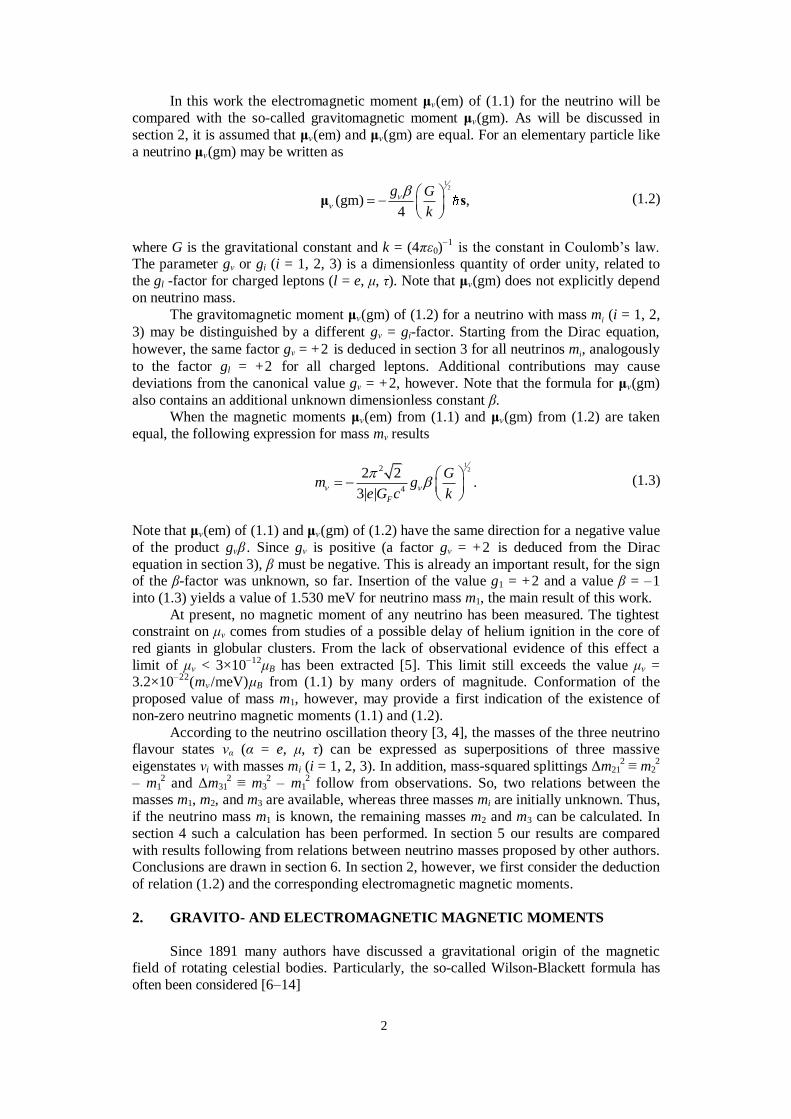
In this work the electromagnetic moment μν(em) of (1.1) for the neutrino will be

compared with the so-called gravitomagnetic moment μν(gm). As will be discussed in

section 2, it is assumed that μν(em) and μν(gm) are equal. For an elementary particle like

a neutrino μν(gm) may be written as

12

(gm) ,4

g G

k

μ s (1.2)

where G is the gravitational constant and k = (4πε0)–1

is the constant in Coulombʼs law. The parameter gν or gi (i = 1, 2, 3) is a dimensionless quantity of order unity, related to

the gl -factor for charged leptons (l = e, μ, τ). Note that μν(gm) does not explicitly depend

on neutrino mass.

The gravitomagnetic moment μν(gm) of (1.2) for a neutrino with mass mi (i = 1, 2,

3) may be distinguished by a different gν = gi-factor. Starting from the Dirac equation,

however, the same factor gν = +2 is deduced in section 3 for all neutrinos mi, analogously

to the factor gl = +2 for all charged leptons. Additional contributions may cause

deviations from the canonical value gν = +2, however. Note that the formula for μν(gm)

also contains an additional unknown dimensionless constant β. When the magnetic moments μν(em) from (1.1) and μν(gm) from (1.2) are taken

equal, the following expression for mass mν results

122

4

2 2.

3| | F

Gm g

e G c k

(1.3)

Note that μν(em) of (1.1) and μν(gm) of (1.2) have the same direction for a negative value

of the product gνβ . Since gν is positive (a factor gν = +2 is deduced from the Dirac

equation in section 3), β must be negative. This is already an important result, for the sign of the β-factor was unknown, so far. Insertion of the value g1 = +2 and a value β = –1

into (1.3) yields a value of 1.530 meV for neutrino mass m1, the main result of this work.

At present, no magnetic moment of any neutrino has been measured. The tightest constraint on μν comes from studies of a possible delay of helium ignition in the core of

red giants in globular clusters. From the lack of observational evidence of this effect a

limit of μν < 3×10–12

μB has been extracted [5]. This limit still exceeds the value μν = 3.2×10

–22(mν /meV)μB from (1.1) by many orders of magnitude. Conformation of the

proposed value of mass m1, however, may provide a first indication of the existence of

non-zero neutrino magnetic moments (1.1) and (1.2).

According to the neutrino oscillation theory [3, 4], the masses of the three neutrino flavour states να (α = e, μ, τ) can be expressed as superpositions of three massive

eigenstates νi with masses mi (i = 1, 2, 3). In addition, mass-squared splittings Δm212 ≡ m2

2

– m12 and Δm31

2 ≡ m3

2 – m1

2 follow from observations. So, two relations between the

masses m1, m2, and m3 are available, whereas three masses mi are initially unknown. Thus,

if the neutrino mass m1 is known, the remaining masses m2 and m3 can be calculated. In

section 4 such a calculation has been performed. In section 5 our results are compared

with results following from relations between neutrino masses proposed by other authors. Conclusions are drawn in section 6. In section 2, however, we first consider the deduction

of relation (1.2) and the corresponding electromagnetic magnetic moments.

2. GRAVITO- AND ELECTROMAGNETIC MAGNETIC MOMENTS

Since 1891 many authors have discussed a gravitational origin of the magnetic field of rotating celestial bodies. Particularly, the so-called Wilson-Blackett formula has

often been considered [6–14]

3

12

(gm) ,2

G

k

μ S (2.1)

where μ(gm) is the gravitomagnetic dipole moment of the massive body with angular

momentum S. For a sphere with a homogeneous mass density the angular momentum S is

given by S = 2/5 mr2ω, where m is the mass of the sphere of radius r and ω its angular

velocity. Note that μ(gm) is proportional to the mass m. The parameter is an unknown dimensionless constant of order unity. See ref. [14] for an ample discussion of its value.

Analogously to its electromagnetic counterpart μ(em) of (1.1), the gravitomagnetic

moment μ(gm) leads to a dipolar gravitomagnetic field at distance R of magnitude

0

5 3

3 (gm) (gm)(gm) .

4 R R

μ R μB R (2.2)

According to the Wilson-Blackett relation, the field B(gm) may be identified as an

electromagnetic induction field. In that case the magnetic moments μ(em) of (1.1) and μ(gm) of (1.2) are equivalent.

Attempts to derive (2.1) from a more general theory have been given by several

authors (see, e.g., [10–15] and references therein). For example, Bennet et al. [10] already gave a five-dimensional theory resulting into (2.1). Luchak [11] found a relation

related to (2.1) by proposing a five-dimensional theory, based on a relativistic

generalization of the Maxwell equations, in order to include gravitational fields. Other

authors like Biemond [12–14] and Widom and Ahluwalia [15], tried to explain equation (2.1) as a consequence of general relativity. The former author [12–14] started from the

Einstein equations in the slow motion and weak field approximation and deduced a set of

four gravitomagnetic equations, analogous to the four Maxwell equations. The so-called “magnetic-type” gravitational field in these equations is identified as a magnetic induction

field, resulting into the gravitomagnetic dipole moment μ(gm) of (2.1).

Since charges in rotating bodies may affect the value of the parameter β in many different ways, one can hardly expect that the observed value of β is a constant. Different

values for the empirical value of β have indeed been found for about fourteen rotating

bodies: metallic cylinders in the laboratory, moons, planets, stars and the Galaxy [13, ch.

1]. For pulsars a separate analysis has been given in ref. [16]. From a linear regression analysis of the series of the fourteen rotating bodies an almost linear relationship between

the observed magnetic moment |μ(obs)| and the angular momentum |S| was found. Such a

linear relationship between μ(gm) and S is predicted by (2.1). From this analysis an average value of |β | = 0.076 was calculated. Although this result is distinctly different

from a gravitomagnetic prediction for a theoretical value like |β | = 1 in (2.1), the correct

order of magnitude of β for so many, strongly different, rotating bodies is amazing (|μ(obs)| and |S| vary over an interval of sixty decades!). So, the gravitomagnetic

hypothesis, embodied in the Wilson-Blackett law (2.1), may basically be valid.

For a macroscopic rotating sphere of mass m with a homogeneous charge density, the

magnetic dipole moment from the total charge Q is given by (see, e.g., ref. [17, 18])

(em) .2

Q

mμ S (2.3)

It is noted that the derivation of (2.3) from the Maxwell equations and the deduction of

(2.1) from the gravitomagnetic equations are analogous. For elementary particles like charged leptons l (l = e, μ, τ) the angular momentum S

is given by S = ½ħs, where s is a unit vector in the direction of S, as has been discussed

4

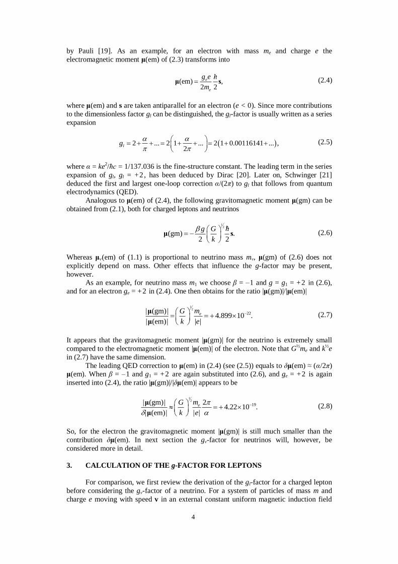
by Pauli [19]. As an example, for an electron with mass me and charge e the

electromagnetic moment μ(em) of (2.3) transforms into

(em) ,2 2

e

e

g e

mμ s (2.4)

where μ(em) and s are taken antiparallel for an electron (e < 0). Since more contributions

to the dimensionless factor gl can be distinguished, the gl-factor is usually written as a series

expansion

2 ... 2 1 ... 2 1 0.00116141 ... ,2

lg

(2.5)

where α = ke

2/ħc = 1/137.036 is the fine-structure constant. The leading term in the series

expansion of gl, gl = +2 , has been deduced by Dirac [20]. Later on, Schwinger [21]

deduced the first and largest one-loop correction α/(2π) to gl that follows from quantum electrodynamics (QED).

Analogous to μ(em) of (2.4), the following gravitomagnetic moment μ(gm) can be

obtained from (2.1), both for charged leptons and neutrinos

12

(gm) .2 2

g G

k

μ s (2.6)

Whereas μν(em) of (1.1) is proportional to neutrino mass mν, μ(gm) of (2.6) does not

explicitly depend on mass. Other effects that influence the g-factor may be present,

however. As an example, for neutrino mass m1 we choose β = –1 and g = g1 = +2 in (2.6),

and for an electron ge = +2 in (2.4). One then obtains for the ratio |μ(gm)|/|μ(em)|

12

22| (gm)|4.899 10 .

| (em)| | |

emG

k e

μ

μ (2.7)

It appears that the gravitomagnetic moment |μ(gm)| for the neutrino is extremely small

compared to the electromagnetic moment |μ(em)| of the electron. Note that G½me and k

½e

in (2.7) have the same dimension.

The leading QED correction to μ(em) in (2.4) (see (2.5)) equals to δμ(em) ≈ (α/2π) μ(em). When β = –1 and g1 = +2 are again substituted into (2.6), and ge = +2 is again

inserted into (2.4), the ratio |μ(gm)|/|δμ(em)| appears to be

12

19| (gm)| 24.22 10 .

| (em)| | |

emG

k e

μ

μ (2.8)

So, for the electron the gravitomagnetic moment |μ(gm)| is still much smaller than the

contribution δμ(em). In next section the gν-factor for neutrinos will, however, be

considered more in detail.

3. CALCULATION OF THE g-FACTOR FOR LEPTONS

For comparison, we first review the derivation of the gl-factor for a charged lepton

before considering the gν-factor of a neutrino. For a system of particles of mass m and

charge e moving with speed v in an external constant uniform magnetic induction field

5

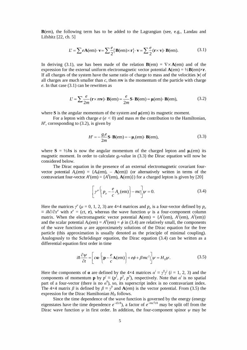
B(em), the following term has to be added to the Lagrangian (see, e.g., Landau and

Lifshitz [22, ch. 5]

(em) (em) ( ) (em).2 2

e eL e A v B r v r v B (3.1)

In deriving (3.1), use has been made of the relation B(em) = A(em) and of the expression for the external uniform electromagnetic vector potential A(em) = ½B(em)×r.

If all charges of the system have the same ratio of charge to mass and the velocities |v| of

all charges are much smaller than c, then mv is the momentum of the particle with charge e. In that case (3.1) can be rewritten as

( ) (em) (em) (em) (em),2 2

e eL m

m m r v B S B μ B (3.2)

where S is the angular momentum of the system and μ(em) its magnetic moment.

For a lepton with charge e (e < 0) and mass m the contribution to the Hamiltonian, H′, corresponding to (3.2), is given by

(em) (em) (em),2

ll

g eH

m S B μ B (3.3)

where S = ½ħs is now the angular momentum of the charged lepton and μl(em) its magnetic moment. In order to calculate gl-value in (3.3) the Dirac equation will now be

considered below.

The Dirac equation in the presence of an external electromagnetic covariant four-

vector potential Aμ(em) = {A0(em), – A(em)} (or alternatively written in terms of the contravariant four-vector A

μ(em) = {A

0(em), A(em)}) for a charged lepton is given by [20]

(em) 0.e

p A mcc

(3.4)

Here the matrices γ

μ (μ = 0, 1, 2, 3) are 4×4 matrices and pμ is a four-vector defined by pμ

≡ iħ∂/∂xμ with x

μ = (ct, r), whereas the wave function ψ is a four-component column

matrix. When the electromagnetic vector potential A(em) = {A1(em), A

2(em), A

3(em)}

and the scalar potential A0(em) = A0(em) = ϕ in (3.4) are relatively small, the components

of the wave functions ψ are approximately solutions of the Dirac equation for the free

particle (this approximation is usually denoted as the principle of minimal coupling). Analogously to the Schrӧdinger equation, the Dirac equation (3.4) can be written as a

differential equation first order in time

2

D(em) .e

i c e mc Ht c

α p A (3.5)

Here the components of α are defined by the 4×4 matrices αi ≡ γ

0γ

i (i = 1, 2, 3) and the

components of momentum p by pi ≡ (p

1, p

2, p

3), respectively. Note that α

i is no spatial

part of a four-vector (there is no α0), so, its superscript index is no contravariant index.

The 4×4 matrix β is defined by β ≡ γ0 and A(em) is the vector potential. From (3.5) the

expression for the Dirac Hamiltonian HD follows.

Since the time dependence of the wave function is governed by the energy (energy

eigenstates have the time dependence e–iEt/ħ

), a factor of e–imc2t/ħ

may be split off from the

Dirac wave function ψ in first order. In addition, the four-component spinor ψ may be

6

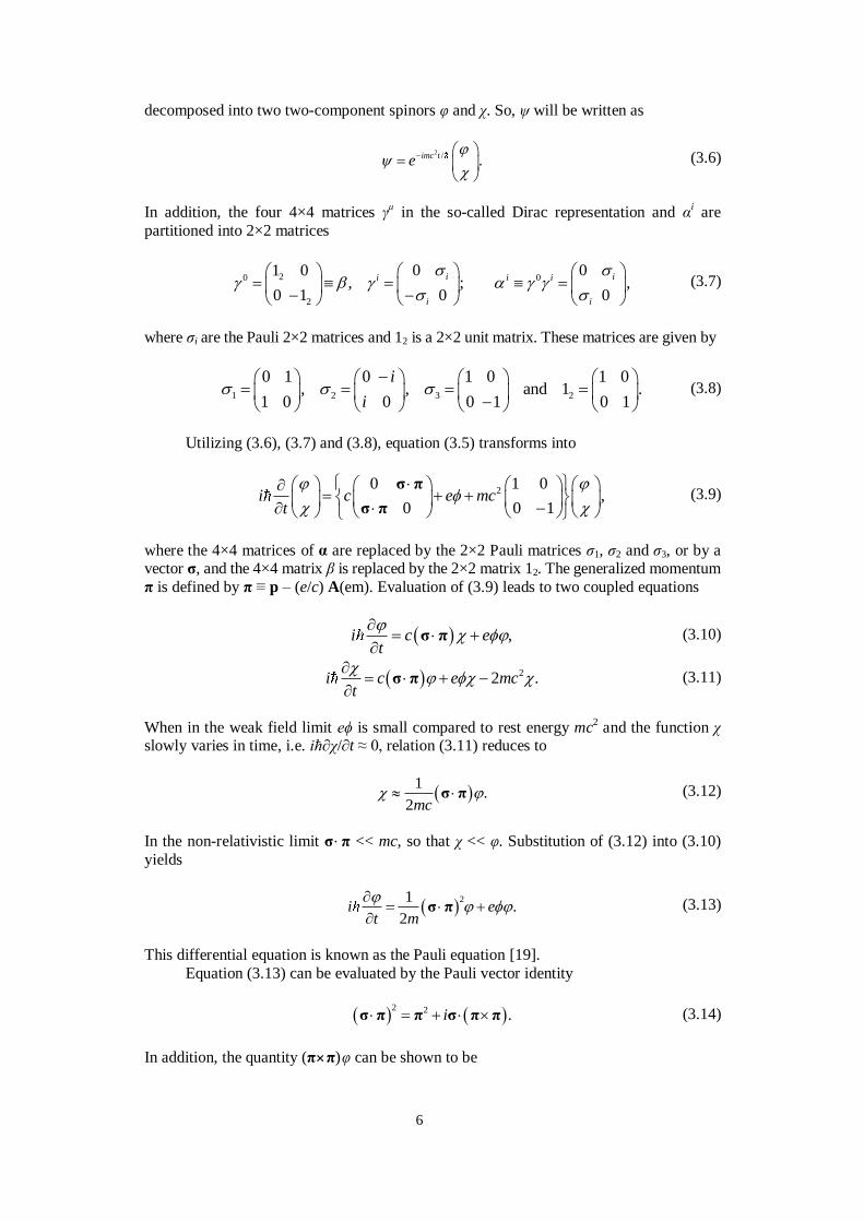
decomposed into two two-component spinors φ and χ. So, ψ will be written as

2 / .imc te

(3.6)

In addition, the four 4×4 matrices γ

μ in the so-called Dirac representation and α

i are

partitioned into 2×2 matrices

20 0

2

0 01 0, ; ,

0 1 0 0

i ii i i

i i

(3.7)

where σi are the Pauli 2×2 matrices and 12 is a 2×2 unit matrix. These matrices are given by

1 2 3 2

0 1 0 1 0 1 0, , and 1 .

1 0 0 0 1 0 1

i

i

(3.8)

Utilizing (3.6), (3.7) and (3.8), equation (3.5) transforms into

20 1 0

,0 0 1

i c e mct

σ π

σ π (3.9)

where the 4×4 matrices of α are replaced by the 2×2 Pauli matrices σ1, σ2 and σ3, or by a vector σ, and the 4×4 matrix β is replaced by the 2×2 matrix 12. The generalized momentum

π is defined by π ≡ p – (e/c) A(em). Evaluation of (3.9) leads to two coupled equations

,i c et

σ π (3.10)

22 .i c e mct

σ π (3.11)

When in the weak field limit eϕ is small compared to rest energy mc2 and the function χ

slowly varies in time, i.e. iħ∂χ/∂t ≈ 0, relation (3.11) reduces to

1

.2mc

σ π (3.12)

In the non-relativistic limit σ π << mc, so that χ << φ. Substitution of (3.12) into (3.10)

yields

21

.2

i et m

σ π (3.13)

This differential equation is known as the Pauli equation [19].

Equation (3.13) can be evaluated by the Pauli vector identity

2 2 .i σ π π σ π π (3.14)

In addition, the quantity (π×π)φ can be shown to be

7

(em) (em) .ie ie π π A B (3.15)

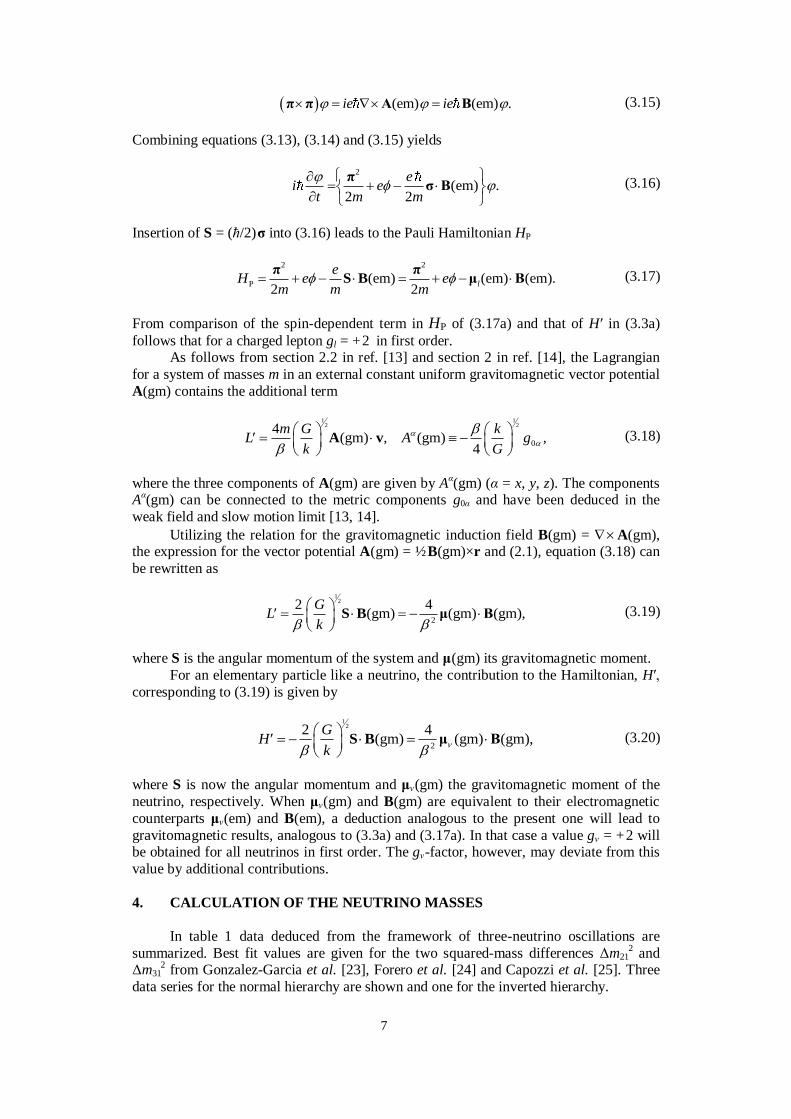
Combining equations (3.13), (3.14) and (3.15) yields

2

(em) .2 2

ei e

t m m

πσ B (3.16)

Insertion of S = (ħ/2)σ into (3.16) leads to the Pauli Hamiltonian HP

2 2

P (em) (em) (em).2 2

l

eH e e

m m m

π πS B μ B (3.17)

From comparison of the spin-dependent term in HP of (3.17a) and that of H′ in (3.3a)

follows that for a charged lepton gl = +2 in first order. As follows from section 2.2 in ref. [13] and section 2 in ref. [14], the Lagrangian

for a system of masses m in an external constant uniform gravitomagnetic vector potential

A(gm) contains the additional term

1 12 2

0

4(gm) , (gm) ,

4

m G kL A g

k G

A v (3.18)

where the three components of A(gm) are given by Aα(gm) (α = x, y, z). The components

Aα(gm) can be connected to the metric components g0α and have been deduced in the

weak field and slow motion limit [13, 14].

Utilizing the relation for the gravitomagnetic induction field B(gm) = A(gm), the expression for the vector potential A(gm) = ½B(gm)×r and (2.1), equation (3.18) can

be rewritten as

12

2

2 4(gm) (gm) (gm),

GL

k

S B μ B (3.19)

where S is the angular momentum of the system and μ(gm) its gravitomagnetic moment.

For an elementary particle like a neutrino, the contribution to the Hamiltonian, H′,

corresponding to (3.19) is given by

12

2

2 4(gm) (gm) (gm),

GH

k

S B μ B (3.20)

where S is now the angular momentum and μν(gm) the gravitomagnetic moment of the

neutrino, respectively. When μν(gm) and B(gm) are equivalent to their electromagnetic

counterparts μν(em) and B(em), a deduction analogous to the present one will lead to

gravitomagnetic results, analogous to (3.3a) and (3.17a). In that case a value gν = +2 will be obtained for all neutrinos in first order. The gν-factor, however, may deviate from this

value by additional contributions.

4. CALCULATION OF THE NEUTRINO MASSES

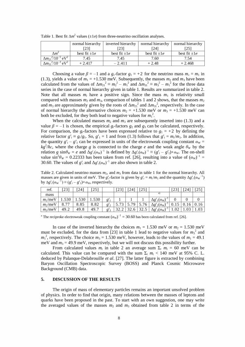
In table 1 data deduced from the framework of three-neutrino oscillations are

summarized. Best fit values are given for the two squared-mass differences Δm212 and

Δm312 from Gonzalez-Garcia et al. [23], Forero et al. [24] and Capozzi et al. [25]. Three

data series for the normal hierarchy are shown and one for the inverted hierarchy.

8

Table 1. Best fit Δm2 values (±1σ) from three-neutrino oscillation analyses.

normal hierarchy

[23]

inverted hierarchy

[23]

normal hierarchy

[24]

normal hierarchy

[25]

Δm2

best fit ±1σ best fit ±1σ best fit ±1σ best fit ±1σ

Δm212/10–5 eV2 7.45 7.45 7.60 7.54

Δm312/10–3 eV2 + 2.417 – 2.411 + 2.48 + 2.468

Choosing a value β = –1 and a gν-factor g1 = +2 for the neutrino mass mν = m1 in (1.3), yields a value of m1 = +1.530 meV. Subsequently, the masses m2 and m3 have been

calculated from the values of Δm212 ≡ m2

2 – m1

2 and Δm31

2 ≡ m3

2 – m1

2 for the three data

series in the case of normal hierarchy given in table 1. Results are summarized in table 2.

Note that all masses mi have a positive sign. Since the mass m1 is relativity small compared with masses m2 and m3, comparison of tables 1 and 2 shows, that the masses m2

and m3 are approximately given by the roots of Δm212 and Δm31

2, respectively. In the case

of normal hierarchy the alternative choices m2 = +1.530 meV or m3 = +1.530 meV can both be excluded, for they both lead to negative values for m1

2.

When the calculated masses m2 and m3 are subsequently inserted into (1.3) and a

value β = –1 is chosen, the empirical gi-factors g2 and g3 can be calculated, respectively. For comparison, the gi-factors have been expressed relative to g1 = +2 by defining the

relative factor g′i ≡ gi /g1. So, g′1 = 1 and from (1.3) follows that g′i = mi /m1. In addition,

the quantity g′i – g′1 can be expressed in units of the electroweak coupling constant αW =

kg2/ħc, where the charge g is connected to the charge e and the weak angle θW by the

relation g sinθW = e and Δg′i (αW)–1 is defined by Δg′i(αW)–1 ≡ (g′i – g′1)×αW. The on-shell

value sin2θW = 0.22333 has been taken from ref. [26], resulting into a value of (αW)–1 =

30.60. The values of g′i and Δg′i (αW)–1 are also shown in table 2. Table 2. Calculated neutrino masses m2, and m3 from data in table 1 for the normal hierarchy. All

masses are given in units of meV. The g′i-factor is given by g′i = mi /m1 and the quantity Δg′i (αW–1)

by Δg′i (αW–1) ≡ (g′i – g′1)×αW, respectively.

ref. [23] [24] [25] [23] [24] [25] [23] [24] [25]

mass a)

m1/meV 1.530 1.530 1.530 g′1 1 1 1 Δg′1(αW)–1 0 0 0

m2/meV 8.77 8.85 8.82 g′2 5.73 5.79 5.76 Δg′2(αW)–1 0.15 0.16 0.16

m3/meV 49.2 49.8 49.7 g′3 32.2 32.6 32.5 Δg′3(αW)–1 1.02 1.03 1.03 a The reciproke electroweak coupling constant (αW)–1 = 30.60 has been calculated from ref. [26].

In case of the inverted hierarchy the choices m1 = 1.530 meV or m2 = 1.530 meV must be excluded, for the data from [23] in table 1 lead to negative values for m3

2 and

m12, respectively. The choice m3 = 1.530 meV, however, leads to the values of m1 = 49.1

meV and m3 = 49.9 meV, respectively, but we will not discuss this possibility further. From calculated values mi in table 2 an average sum Σi mi = 60 meV can be

calculated. This value can be compared with the sum Σi mi < 140 meV at 95% C. L.

deduced by Palanque-Delabrouille et al. [27]. The latter figure is extracted by combining Baryon Oscillation Spectroscopic Survey (BOSS) and Planck Cosmic Microwave

Background (CMB) data.

5. DISCUSSION OF THE RESULTS

The origin of mass of elementary particles remains an important unsolved problem

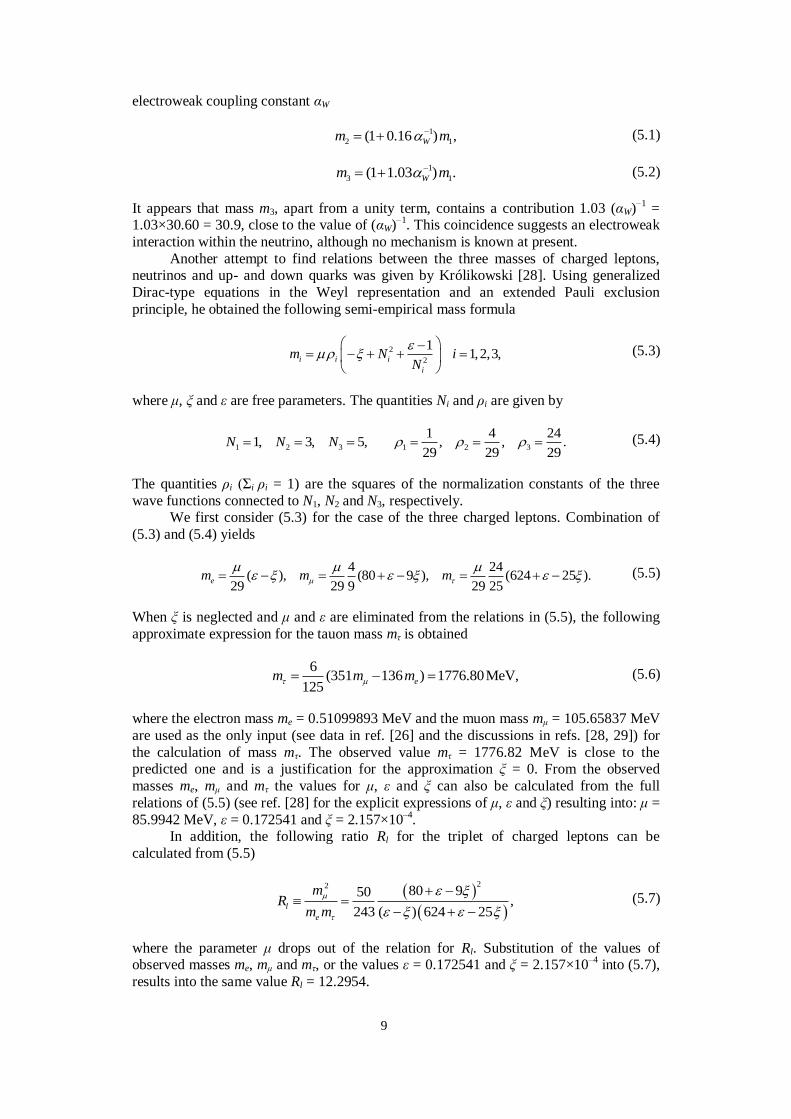
of physics. In order to find that origin, many relations between the masses of leptons and quarks have been proposed in the past. To start with an own suggestion, one may write

the averaged values of the masses m2 and m3 obtained from table 2 in terms of the

9

electroweak coupling constant αW

1

2 1(1 0.16 ) ,Wm m (5.1)

1

3 1(1 1.03 ) .Wm m (5.2)

It appears that mass m3, apart from a unity term, contains a contribution 1.03 (αW)–1

= 1.03×30.60 = 30.9, close to the value of (αW)

–1. This coincidence suggests an electroweak

interaction within the neutrino, although no mechanism is known at present.

Another attempt to find relations between the three masses of charged leptons, neutrinos and up- and down quarks was given by Królikowski [28]. Using generalized

Dirac-type equations in the Weyl representation and an extended Pauli exclusion

principle, he obtained the following semi-empirical mass formula

2

2

11,2,3,i i i

i

m N iN

(5.3)

where μ, ξ and ε are free parameters. The quantities Ni and ρi are given by

1 2 3 1 2 3

1 4 241, 3, 5, , , .

29 29 29N N N (5.4)

The quantities ρi (Σi ρi = 1) are the squares of the normalization constants of the three

wave functions connected to N1, N2 and N3, respectively. We first consider (5.3) for the case of the three charged leptons. Combination of

(5.3) and (5.4) yields

4 24( ), (80 9 ), (624 25 ).

29 29 9 29 25em m m

(5.5)

When ξ is neglected and μ and ε are eliminated from the relations in (5.5), the following

approximate expression for the tauon mass mτ is obtained

6

(351 136 ) 1776.80MeV,125

em m m (5.6)

where the electron mass me = 0.51099893 MeV and the muon mass mμ = 105.65837 MeV

are used as the only input (see data in ref. [26] and the discussions in refs. [28, 29]) for

the calculation of mass mτ. The observed value mτ = 1776.82 MeV is close to the predicted one and is a justification for the approximation ξ = 0. From the observed

masses me, mμ and mτ the values for μ, ε and ξ can also be calculated from the full

relations of (5.5) (see ref. [28] for the explicit expressions of μ, ε and ξ) resulting into: μ =

85.9942 MeV, ε = 0.172541 and ξ = 2.157×10–4

. In addition, the following ratio Rl for the triplet of charged leptons can be

calculated from (5.5)

2280 950

,243 ( ) 624 25

l

e

mR

m m

(5.7)

where the parameter μ drops out of the relation for Rl. Substitution of the values of observed masses me, mμ and mτ, or the values ε = 0.172541 and ξ = 2.157×10

–4 into (5.7),

results into the same value Rl = 12.2954.

10

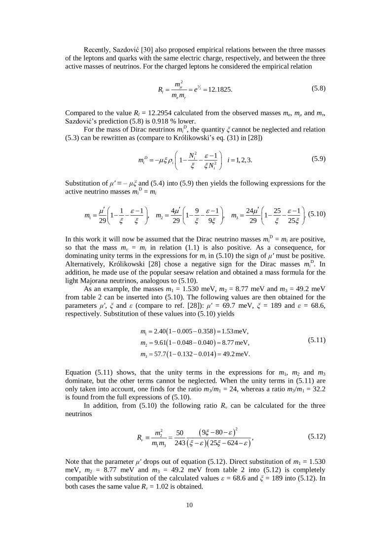
Recently, Sazdović [30] also proposed empirical relations between the three masses

of the leptons and quarks with the same electric charge, respectively, and between the three

active masses of neutrinos. For the charged leptons he considered the empirical relation

52

2

12.1825.l

e

mR e

m m

(5.8)

Compared to the value Rl = 12.2954 calculated from the observed masses me, mμ and mτ,

Sazdović’s prediction (5.8) is 0.918 % lower. For the mass of Dirac neutrinos mi

D, the quantity ξ cannot be neglected and relation

(5.3) can be rewritten as (compare to Królikowski’s eq. (31) in [28])

2

2

11 1,2,3.D i

i i

i

Nm i

N

(5.9)

Substitution of μ' ≡ – μξ and (5.4) into (5.9) then yields the following expressions for the

active neutrino masses miD = mi

1 2 3

1 1 4 9 1 24 25 11 , 1 , 1 .

29 29 9 29 25m m m

(5.10)

In this work it will now be assumed that the Dirac neutrino masses miD = mi are positive,

so that the mass mν = mi in relation (1.1) is also positive. As a consequence, for dominating unity terms in the expressions for mi in (5.10) the sign of μ' must be positive.

Alternatively, Królikowski [28] chose a negative sign for the Dirac masses miD. In

addition, he made use of the popular seesaw relation and obtained a mass formula for the

light Majorana neutrinos, analogous to (5.10). As an example, the masses m1 = 1.530 meV, m2 = 8.77 meV and m3 = 49.2 meV

from table 2 can be inserted into (5.10). The following values are then obtained for the

parameters μ', ξ and ε (compare to ref. [28]): μ' = 69.7 meV, ξ = 189 and ε = 68.6, respectively. Substitution of these values into (5.10) yields

1

2

3

2.40 1 0.005 0.358 1.53meV,

9.61 1 0.048 0.040 8.77 meV,

57.7 1 0.132 0.014 49.2meV.

m

m

m

(5.11)

Equation (5.11) shows, that the unity terms in the expressions for m1, m2 and m3

dominate, but the other terms cannot be neglected. When the unity terms in (5.11) are

only taken into account, one finds for the ratio m3/m1 = 24, whereas a ratio m3/m1 = 32.2 is found from the full expressions of (5.10).

In addition, from (5.10) the following ratio Rν can be calculated for the three

neutrinos

22

2

1 3

9 8050,

243 25 624

mR

m m

(5.12)

Note that the parameter μ' drops out of equation (5.12). Direct substitution of m1 = 1.530 meV, m2 = 8.77 meV and m3 = 49.2 meV from table 2 into (5.12) is completely

compatible with substitution of the calculated values ε = 68.6 and ξ = 189 into (5.12). In

both cases the same value Rν = 1.02 is obtained.

11

For the triplet of neutrinos Sazdović [30] proposed the simple relation

2

2

1 3

1,                                                              m

Rm m

(5.13)

without giving a theoretical basis for this relation. The ratio (5.13) provides a third

relation between the masses m1, m2 and m3, so that all masses can be calculated. Choosing

the values for Δm212 and Δm31

2 for the normal hierarchy from [23] in our table 1, the

following results can be calculated from (5.13): m1 = 1.56 meV, m2 = 8.77 meV and m3 =

49.2 meV, close to the values following from our approach and given in our table 2. The

proposed ratio Rν = 1 almost equals to the value Rν = 1.02 from (5.12), calculated from m1

= 1.530 meV and Δm212 and Δm31

2 data for the normal hierarchy from [23] in our table 1.

Instead of introducing β = –1 into (1.3), one might choose a value like β = –2. In

that case the value of m1 doubles to m1 = 3.06 meV. Combination of this value for m1 and

data from [23] in table 1 yields the values m2 = 9.16 meV and m3 = 49.3 meV. In that case a value of Rν = 0.56 follows from (5.12). If Sazdović ’s relation (5.13) is approximately

valid, however, the choice β = –2 must be rejected, whereas the value β = –1 is

acceptable. Królikowski [28] and Sazdović [30] also gave related expressions for the masses of

the up- and down quarks. Since the masses of the quarks are less accurately known in

general, we will not consider these relations further.

6. CONCLUSIONS

A value of 1.530 meV/c2 = 2.727×10

–39 kg for the mass of the lightest neutrino m1

is obtained in this work. This value is extracted from a combination of the magnetic

moment of a massive Dirac neutrino [1, 2], deduced in the context of electroweak

interactions at the one-loop level, ànd the magnetic moment from gravitational origin

proposed by Wilson and Blackett [6–12]. The latter relation has also been obtained from a gravitomagnetic interpretation of the Einstein equations [12–14]. Combination with

neutrino oscillation data yields the other masses m2 and m3 (see table 2). Note that the

ratio m3/m1 is in the range of the reciprocal value of the electroweak coupling constant. Our results for the neutrino masses are compatible with the three-parameter semi-

empirical neutrino mass formulas deduced by Królikowski [28], utilizing generalized

Dirac-type equations in the Weyl representation and an extended Pauli exclusion principle. Sazdović [30] recently proposed the empirical relation Rν = (m2)

2/(m1m3) = 1 for

the three active masses of the neutrinos and found about the same set of masses m1, m2

and m3 obtained in this work. From Królikowski’s theoretical treatment also follows an

expression for Rν. His approach and ours yield the same value Rν = 1.02, when our set of neutrino masses is chosen. It is remarkable that three different approaches lead to about

the same value of Rν.

REFERENCES

[1] Lee, B. W. and Shrock, R. E., "Natural suppression of symmetry violation in gauge theories: muon- and

electron-lepton-number nonconservation", Phys. Rev. D 16, 1444-1473 (1977). [2] Fujikawa, K. and Shrock, R. E., "Magnetic moment of a massive neutrino and neutrino-spin rotation",

Phys. Rev. Letters 45, 963-966 (1980) and references therein. [3] Maki, Z., Nakagawa, M. and Sakata, S., "Remarks on the unified model of elementary particles", Prog.

Theor. Phys. 28, 870-880 (1962).

[4] Kobayashi, M. and Maskawa, T., "CP violation in the renormalizable theory of weak interaction.", Prog. Theor. Phys. 49, 652-657 (1973).

[5] Raffelt, G. G., "New bound on neutrino dipole moments from globular-cluster stars", Phys. Rev. Lett., 64, 2856-2858 (1990).

12

[6] Schuster, A., "A critical examination of the possible causes of terrestrial magnetism", Proc. Phys. Soc.

Lond. 24, 121-137 (1912). [7] Wilson, H. A., "An experiment on the origin of the Earth's magnetic field", Proc. R. Soc. Lond. A 104,

451-455 (1923). [8] Blackett, P. M. S., "The magnetic field of massive rotating bodies", Nature 159, 658-666 (1947). [9] Sirag, S-P., "Gravitational magnetism", Nature 278, 535-538 (1979). [10] Bennett, J. G., Brown, R. L. and Thring, M. W., "Unified field theory in a curvature-free five-

dimensional manifold", Proc. R. Soc. Lond. A 198, 39-61(1949). [11] Luchak, G., "A fundamental theory of the magnetism of massive rotating bodies", Can. J. Phys. 29,

470-479 (1951). [12] Biemond, J., Gravi-magnetism, 1st ed. (1984). Postal address: Sansovinostraat 28, 5624 JX Eindhoven,

The Netherlands. E-mail: j.biemond@gravito.nl Website: http://www.gravito.nl [13] Biemond, J., Gravito-magnetism, 2nd ed. (1999). See also ref. [12]. [14] Biemond, J., "Which gravitomagnetic precession rate will be measured by Gravity Probe B?",

arXiv:physics/0411129v1 [physics.gen-ph], 13 Nov 2004. [15] Widom, A. and Ahluwalia, D. V., "Magnetic moments of astrophysical objects as a consequence of

general relativity", Chin. J. Phys. 25, 23-26 (1987). [16] Biemond, J., "The origin of the magnetic field of pulsars and the gravitomagnetic theory". In: Trends in

pulsar research (Ed. Lowry, J. A.), Nova Science Publishers, New York, Chapter 2 (2007) (updated and revised version of arXiv:astro-ph/0401468v1, 22 Jan 2004).

[17] Biemond, J., "Quasi-periodic oscillations, charge and the gravitomagnetic theory", arXiv:0706.0313v2 [physics.gen-ph], 20 Mar 2009.

[18] Biemond, J., "The gravitomagnetic field of a sphere, Gravity Probe B and the LAGEOS satellites", arXiv:physics/0802.3346v2 [physics.gen-ph], 14 Jan 2012.

[19] Pauli, W., "Zur Quantenmechanik des magnetischen Elektrons", Zeit. f. Phys. 43, 601-623 (1927). [20] Dirac, P. A. M., "The quantum theory of the electron", Proc. R. Soc. Lond. A 117, 610-624 (1928).

[21] Schwinger, J., "On quantum-electrodynamics and the magnetic moment of the electron", Phys. Rev., 73, 416-417 (1948).

[22] Landau, L. D. and Lifshitz, E. M., The classical theory of fields, 4th rev. ed., Pergamon Press, Oxford (1975).

[23] Gonzalez-Garcia, M. C. "Global analyses of oscillation neutrino experiments", Phys. Dark Universe 4, 1-5 (2014). See also: Gonzalez-Garcia, M. C., Maltoni, M. and Schwetz, T. "Updated fit to three neutrino mixing: status of leptonic CP violation", J. High Energy Phys., 11, 052, (2014); arXiv:1409.5439v2 [hep-ph], 16 Dec 2014.

[24] Forero, D. V., Tórtola, M. and Valle, J. W. F. "Neutrino oscillations refitted", Phys. Rev. D 90, 093006 (2014); arXiv:1405.7540v3 [hep-ph], 21 Nov 2014.

[25] Capozzi, F., Fogli, G. L., Lisi, E., Marrone, A., Montanino, D. and Pallazo, A. "Status of three-neutrino oscillation parameters, circa 2013", Phys. Rev. D 89, 093018 (2014); arXiv:1312.2878v2 [hep-ph], 5 May 2014.

[26] Olive, K. A, et al. (Particle Data Group), Chin. Phys. C 38, 090001 (2014) Website: http://pdg.lbl.gov/ [27] Palanque-Delabrouille, N., Yèche, C., Lesgourgues, J. et al. "Constraint on neutrino masses from

SDSS-III/BOSS Lyα forest and other cosmological probes", J. Cosmol. Astropart. Phys. 02, 045

(2015); arXiv:1410.7744v2 [astro-ph.CO], 12 Jan 2015. [28] Królikowski, W., "A universal shape of empirical mass formula for all leptons and quarks", Acta Phys.

Pol. B 37, 2601-2613 (2006) and references therein. [29] Królikowski, W., "How the tau-lepton mass can be understood", arXiv:1009.2388v2 [hep-ph], 24 Sep

2010. [30] Sazdović, B., "Charge dependent relation between the masses of different generations and neutrino

masses", arXiv:1501.07617v1 [hep-ph], 29 Jan 2015.