Mussa Puzzle Redux - Princeton University

Mussa Puzzle Redux

Oleg Itskhoki Dmitry Mukhin

[email protected] [email protected]

Princeton UniversityMarch, 2019

1 / 30

mailto:[email protected]

mailto:[email protected]

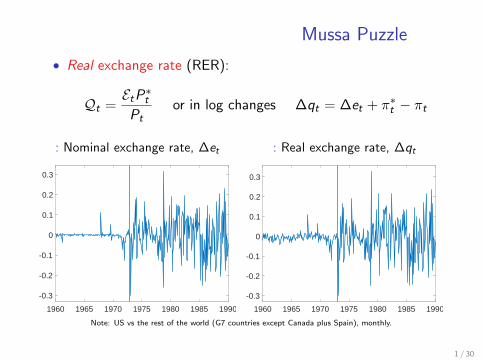
Mussa Puzzle

• Real exchange rate (RER):

Qt =EtP∗

t

Ptor in log changes ∆qt = ∆et + π∗t − πt

: Nominal exchange rate, ∆et

1960 1965 1970 1975 1980 1985 1990

-0.3

-0.2

-0.1

0

0.1

0.2

0.3

: Real exchange rate, ∆qt

1960 1965 1970 1975 1980 1985 1990

-0.3

-0.2

-0.1

0

0.1

0.2

0.3

Note: US vs the rest of the world (G7 countries except Canada plus Spain), monthly.

1 / 30

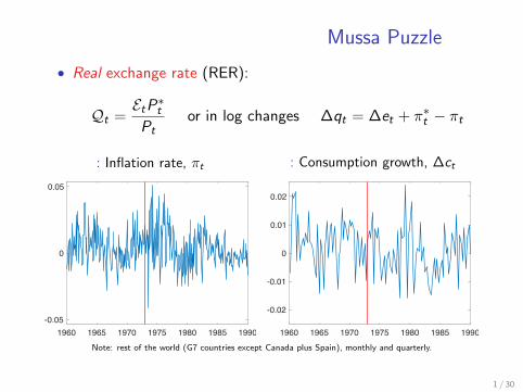
Mussa Puzzle

• Real exchange rate (RER):

Qt =EtP∗

t

Ptor in log changes ∆qt = ∆et + π∗t − πt

: Inflation rate, πt

1960 1965 1970 1975 1980 1985 1990-0.05

0

0.05

: Consumption growth, ∆ct

1960 1965 1970 1975 1980 1985 1990

-0.02

-0.01

0

0.01

0.02

Note: rest of the world (G7 countries except Canada plus Spain), monthly and quarterly.

1 / 30

Mussa Puzzle Redux• Mussa puzzle is some of the most convincing evidence for

monetary non-neutrality (Nakamura and Steinsson, 2018)

— with monetary neutrality, real exchanger rate should not beaffected by a change in the monetary rule

— timing and the sharp discontinuity in the behavior of ERs

• Mussa fact is further interpreted as direct evidence in favor ofnominal rigidities in price setting (sticky prices)

• We argue this latter conclusion is not supported by the data:

no contemporaneous change in properties of macro variables

1 neither nominal, like inflation

2 nor real, like consumption, output or net exports

Is it an extreme form of neutrality? or disconnect?

• The combined evidence does not favor sticky prices overflexible prices, but rather rejects both types of models

2 / 30

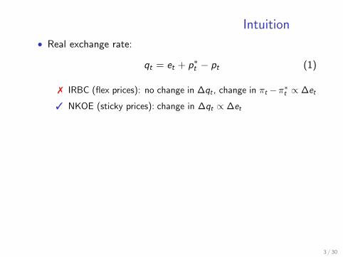
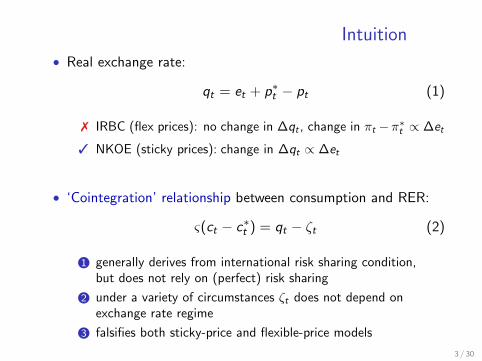
Intuition

• Real exchange rate:

qt = et + p∗t − pt (1)

7 IRBC (flex prices): no change in ∆qt , change in πt −π∗t ∝ ∆et

3 NKOE (sticky prices): change in ∆qt ∝ ∆et

• ‘Cointegration’ relationship between consumption and RER:

ς(ct − c∗t ) = qt − ζt (2)

1 generally derives from international risk sharing condition,but does not rely on (perfect) risk sharing

2 under a variety of circumstances ζt does not depend onexchange rate regime

3 falsifies both sticky-price and flexible-price models

3 / 30

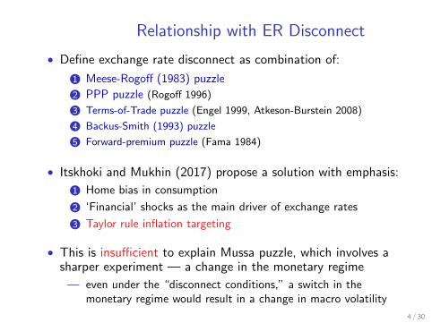
Relationship with ER Disconnect

• Define exchange rate disconnect as combination of:

1 Meese-Rogoff (1983) puzzle

2 PPP puzzle (Rogoff 1996)

3 Terms-of-Trade puzzle (Engel 1999, Atkeson-Burstein 2008)

4 Backus-Smith (1993) puzzle

5 Forward-premium puzzle (Fama 1984)

• Itskhoki and Mukhin (2017) propose a solution with emphasis:

1 Home bias in consumption

2 ‘Financial’ shocks as the main driver of exchange rates

3 Taylor rule inflation targeting

• This is insufficient to explain Mussa puzzle, which involves asharper experiment — a change in the monetary regime

— even under the “disconnect conditions,” a switch in themonetary regime would result in a change in macro volatility

4 / 30

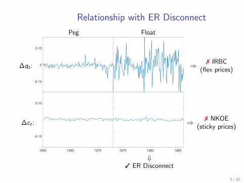
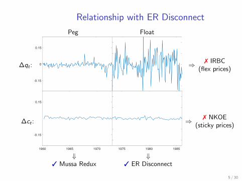
Relationship with ER Disconnect

Peg Float

∆qt :

-0.15

0

0.15

⇒ 7 IRBC(flex prices)

∆ct :

1960 1965 1970

-0.15

0.15

1975 1980 1985

⇒ 7 NKOE(sticky prices)

⇓3 Mussa Redux

⇓3 ER Disconnect

5 / 30

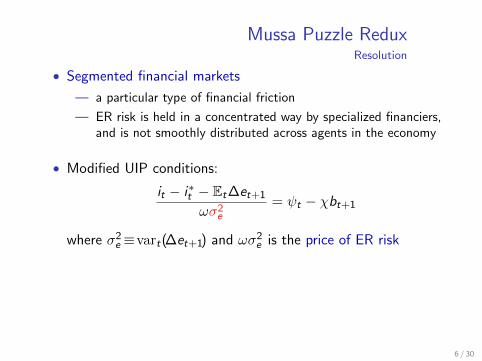
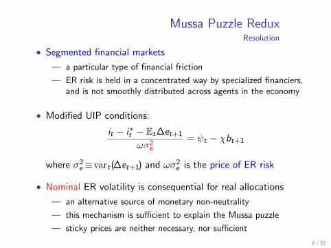
Mussa Puzzle ReduxResolution

• Segmented financial markets

— a particular type of financial friction

— ER risk is held in a concentrated way by specialized financiers,and is not smoothly distributed across agents in the economy

• Modified UIP conditions:

it − i∗t − Et∆et+1

ωσ2e

= ψt − χbt+1

where σ2e ≡vart(∆et+1) and ωσ2

e is the price of ER risk

• Nominal ER volatility is consequential for real allocations

— an alternative source of monetary non-neutrality

— this mechanism is sufficient to explain the Mussa puzzle

— sticky prices are neither necessary, nor sufficient

6 / 30

Related literature

• Empirics:

— Mussa (1986), Baxter and Stockman (1989),Flood and Rose (1995)

• Theory:

— Jeanne and Rose (2002), Monacelli (2004), Kollmann (2005),Alvarez, Atkeson and Kehoe (2007)

• Additional empirical moments:

— Colacito and Croce (2013), Devereux and Hnatkovska (2014),Berka, Devereux and Engel (2018)

7 / 30

EMPIRICAL PATTERNS

8 / 30

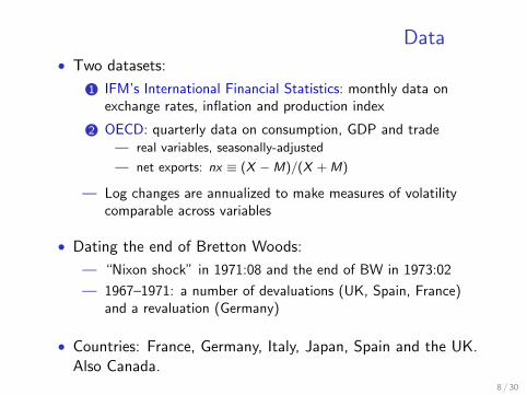
Data• Two datasets:

1 IFM’s International Financial Statistics: monthly data onexchange rates, inflation and production index

2 OECD: quarterly data on consumption, GDP and trade— real variables, seasonally-adjusted

— net exports: nx ≡ (X −M)/(X + M)

— Log changes are annualized to make measures of volatilitycomparable across variables

• Dating the end of Bretton Woods:

— “Nixon shock” in 1971:08 and the end of BW in 1973:02

— 1967–1971: a number of devaluations (UK, Spain, France)and a revaluation (Germany)

• Countries: France, Germany, Italy, Japan, Spain and the UK.Also Canada.

8 / 30

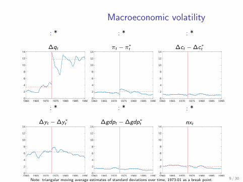
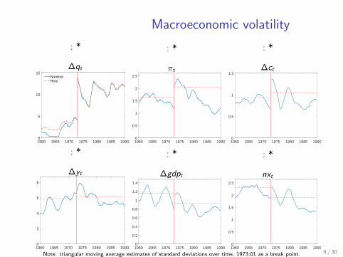
Macroeconomic volatility

: *

∆qt

1960 1965 1970 1975 1980 1985 1990

0

2

4

6

8

10

12

14

: *

πt − π∗t

1960 1965 1970 1975 1980 1985 19900

2

4

6

8

10

12

14

: *

∆ct − ∆c∗t

1960 1965 1970 1975 1980 1985 19900

2

4

6

8

10

12

14

: *

∆yt − ∆y∗t

1960 1965 1970 1975 1980 1985 19900

2

4

6

8

10

12

14

: *

∆gdpt − ∆gdp∗t

1960 1965 1970 1975 1980 1985 19900

2

4

6

8

10

12

14

: *

nxt

1960 1965 1970 1975 1980 1985 19900

2

4

6

8

10

12

14

Note: triangular moving average estimates of standard deviations over time, 1973:01 as a break point. 9 / 30


: *

∆qt

1960 1965 1970 1975 1980 1985 19900

5

10

15NominalReal

: *

πt − π∗t

1960 1965 1970 1975 1980 1985 19900

0.5

1

1.5

2

2.5

3

: *

∆ct − ∆c∗t

1960 1965 1970 1975 1980 1985 19900

0.5

1

1.5

: *

∆yt − ∆y∗t

1960 1965 1970 1975 1980 1985 19900

2

4

6

8

: *

∆gdpt − ∆gdp∗t

1960 1965 1970 1975 1980 1985 19900

0.5

1

1.5

: *

nxt

1960 1965 1970 1975 1980 1985 19900

0.5

1

1.5

2

2.5



: *

∆qt

1960 1965 1970 1975 1980 1985 19900

5

10

15NominalReal

: *

πt

1960 1965 1970 1975 1980 1985 19900

0.5

1

1.5

2

2.5

: *

∆ct

1960 1965 1970 1975 1980 1985 19900

0.5

1

1.5

: *

∆yt

1960 1965 1970 1975 1980 1985 19900

2

4

6

8

: *

∆gdpt

1960 1965 1970 1975 1980 1985 19900

0.2

0.4

0.6

0.8

1

1.2

1.4

: *

nxt

1960 1965 1970 1975 1980 1985 19900

0.5

1

1.5

2

2.5


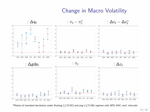
Change in Macro Volatility

: ∆qt

CAN FRA GER ITA JAP SPA UK RoW

0

1

2

3

4

5

6

7

8

: πt − π∗t


0

1

2

3

4

5

6

7

8

: ∆ct −∆c∗t


0

1

2

3

4

5

6

7

8

: ∆gdpt

CAN FRA GER ITA JAP SPA UK US RoW

0

1

2

3

4

5

6

7

8

: πt


0

1

2

3

4

5

6

7

8

: ∆ct


0

1

2

3

4

5

6

7

8

*Ratios of standard deviations under floating (≥73:02) and peg (≤71:08) regimes with 90% HAC conf. intervals

10 / 30

Correlations

: (∆qt ,∆et)

1960 1965 1970 1975 1980 1985 1990-0.2

0

0.2

0.4

0.6

0.8

1: (•, πt − π∗t )

1960 1965 1970 1975 1980 1985 1990-1

-0.5

0

0.5

1

Note: Triangular moving average correlations, treating 1973:01 as the end point for the two regimest

11 / 30

CONVETIONAL MODELS:

FALSIFICATION

12 / 30

‘Conventional’ Models• Definition: if prices were flexible, a switch in the monetary

regime would not affect real variables

— hence, only sticky-price version can be considered

• Log-linear approximate solution— ‘conventional’— second-order (risk premia) terms are small— we allow for risk-sharing wedges instead

• Two-country New Keynesian Open Economy model

◦ with producer-currency (PCP) Calvo price stickiness

◦ with productivity and ‘financial’ shocks

◦ flexible wages, no capital, no intermediates

• Monetary policy (‘primal approach’):

◦ Foreign: inflation targeting π∗t ≡ 0

◦ Home: ‘float’ is πt ≡ 0 and ‘peg’ is ∆et ≡ 0

12 / 30

Model setup I• Households:

maxE0

∑∞

t=0βt

(1

1− σC 1−σt − 1

1 + ϕL1+ϕt

)s.t. PtCt +

∑j∈Jt

ΘjtB

jt+1 ≤WtLt +

∑j∈Jt−1

e−ζjtD j

tBjt + Πt + Tt

◦ CES aggregator across products with elasticity θ > 1

◦ home bias with expenditure share on foreign varieties γ ∈ (0, 12 )

• Optimality conditions:

Cσt Lϕt = Wt/Pt ,

CFt(i) = γe ξt(PFt(it)

Pt

)−θCt ,

Θjt = βEt

{(Ct+1

Ct

)−σPt

Pt+1e−ζ

jt+1D j

t+1

}and PtCt = PHtCHt + PFtCFt

13 / 30

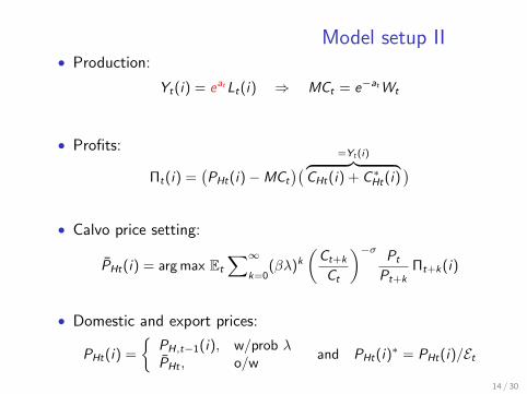
Model setup II• Production:

Yt(i) = eatLt(i) ⇒ MCt = e−atWt

• Profits:

Πt(i) =(PHt(i)−MCt

)( =Yt(i)︷︸︸︷CHt(i) + C∗Ht(i)

)• Calvo price setting:

PHt(i) = arg max Et

∑∞

k=0(βλ)k

(Ct+k

Ct

)−σPt

Pt+kΠt+k(i)

• Domestic and export prices:

PHt(i) =

{PH,t−1(i), w/prob λPHt , o/w

and PHt(i)∗ = PHt(i)/Et

14 / 30

International Equilibrium1 International risk sharing

— for j ∈ Jt ∩ J∗t

Et

{[(Ct+1

Ct

)−σ−(C∗t+1

C∗t

)−σ Qt

Qt+1e ζ

jt+1

]D j

t+1

Pt+1/Pt

}= 0

2 Country budget constraint

Bt+1−RtBt =

=NXt︷︸︸︷PHtC

∗Ht − EtP∗FtCFt =

γPθt Ct

(EtP∗Ft)θ−1

[e ξtSθ−1

t QθtC∗tCt− 1

]— where Bt+1 ≡

∑j∈Jt Θj

tBjt+1 is NFA position

— terms of trade St ≡ EtP∗Ft

PHt≈ Q

11−2γ

t

3 Open economy Phillips curve

— another relationship that links Ct/C∗t and Qt

— only condition that directly depends on the monetary regime

15 / 30

International Equilibrium1 International risk sharing — for j ∈ Jt ∩ J∗t

Et

{[(Ct+1

Ct

)−σ−(C∗t+1

C∗t

)−σ Qt

Qt+1e ζ

jt+1

]D j

t+1

Pt+1/Pt

}= 0

2 Country budget constraint

Bt+1−RtBt =

=NXt︷︸︸︷PHtC

∗Ht − EtP∗FtCFt =

γPθt Ct

(EtP∗Ft)θ−1

[e ξtSθ−1

t QθtC∗tCt− 1

]— where Bt+1 ≡

∑j∈Jt Θj

tBjt+1 is NFA position

— terms of trade St ≡ EtP∗Ft

PHt≈ Q

11−2γ

t

3 Open economy Phillips curve

— another relationship that links Ct/C∗t and Qt

— only condition that directly depends on the monetary regime

15 / 30

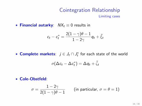
Cointegration RelationshipLimiting cases

• Financial autarky: NXt ≡ 0 results in

ct − c∗t =2(1− γ)θ − 1

1− 2γqt + ξt

• Complete markets: j ∈ Jt ∩ J∗t for each state of the world

σ(∆ct −∆c∗t ) = ∆qt + ζt

• Cole-Obstfeld:

σ =1− 2γ

2(1− γ)θ − 1(in particular, σ = θ = 1)

16 / 30

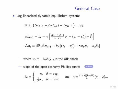
General Case

• Log-linearized dynamic equilibrium system:

Et

{σ(∆ct+1 −∆c∗t+1)−∆qt+1

}= ψt ,

βbt+1 − bt = γ[

2(1−γ)θ−11−2γ qt − (ct − c∗t ) + ξt

]∆qt = βEt∆qt+1 − kR

[(ct − c∗t ) + γκqqt − κaat

]— where ψt ≡ −Et∆ζt+1 is the UIP shock

— slope of the open economy Phillips curve: show

kR =

{κ, R = peg

12γκ, R = float

and κ = (1−λ)(1−βλ)λ (σ + ϕ)...

17 / 30

General Case

• Log-linearized dynamic equilibrium system:

σ(ct − c∗t )− qt = − ψt

1− ρ+ mt , ∆mt = ut

βbt+1 − bt = γ[

2(1−γ)θ−11−2γ qt − (ct − c∗t ) + ξt

]∆qt = βEt∆qt+1 − kR


]— where ψt ≡ −Et∆ζt+1 is the UIP shock

— slope of the open economy Phillips curve: show

kR =

{κ, R = peg

12γκ, R = float

and κ = (1−λ)(1−βλ)λ (σ + ϕ)...

17 / 30

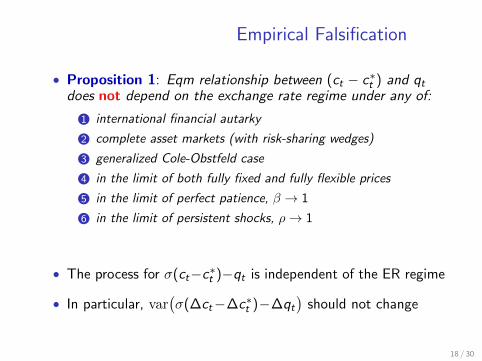
Empirical Falsification

• Proposition 1: Eqm relationship between (ct − c∗t ) and qtdoes not depend on the exchange rate regime under any of:

1 international financial autarky

2 complete asset markets (with risk-sharing wedges)

3 generalized Cole-Obstfeld case

4 in the limit of both fully fixed and fully flexible prices

5 in the limit of perfect patience, β → 1

6 in the limit of persistent shocks, ρ→ 1

• The process for σ(ct−c∗t )−qt is independent of the ER regime

• In particular, var(σ(∆ct−∆c∗t )−∆qt

)should not change

18 / 30

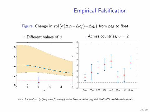
Empirical Falsification

Figure: Change in std(σ(∆ct−∆c∗t )−∆qt

)from peg to float

: Different values of σ : Across countries, σ = 2

CAN FRA GER ITA JAP SPA UK RoW0

1

2

3

4

5

6

7

8

Note: Ratio of std(σ(∆ct−∆c∗t )−∆qt

)under float vs under peg with HAC 90% confidence intervals

19 / 30

ALTERNATIVE MODEL OFNON-NEUTRALITY

20 / 30

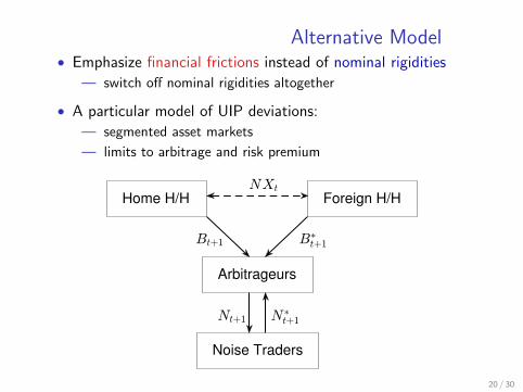
Alternative Model• Emphasize financial frictions instead of nominal rigidities

— switch off nominal rigidities altogether

• A particular model of UIP deviations:

— segmented asset markets

— limits to arbitrage and risk premium

Home H/H Foreign H/H

Noise Traders

Arbitrageurs

20 / 30

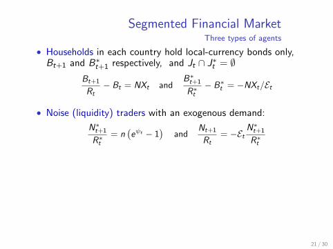
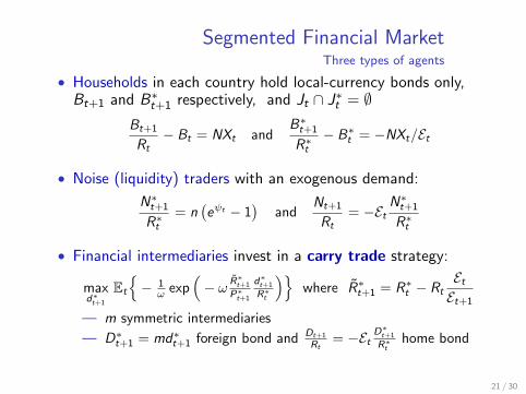
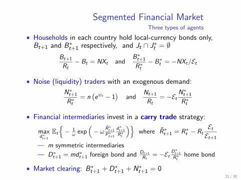
Segmented Financial MarketThree types of agents

• Households in each country hold local-currency bonds only,Bt+1 and B∗

t+1 respectively, and Jt ∩ J∗t = ∅Bt+1

Rt− Bt = NXt and

B∗t+1

R∗t− B∗t = −NXt/Et

• Noise (liquidity) traders with an exogenous demand:

N∗t+1

R∗t= n

(eψt − 1

)and

Nt+1

Rt= −Et

N∗t+1

R∗t

• Financial intermediaries invest in a carry trade strategy:

maxd∗t+1

Et

{− 1

ω exp(− ω R∗

t+1

P∗t+1

d∗t+1

R∗t

)}where R∗t+1 = R∗t − Rt

EtEt+1

— m symmetric intermediaries

— D∗t+1 = md∗t+1 foreign bond and Dt+1

Rt= −Et

D∗t+1

R∗t

home bond

• Market clearing: B∗t+1 + D∗

t+1 + N∗t+1 = 0

21 / 30

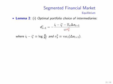
Segmented Financial MarketEquilibrium

• Lemma 2: (i) Optimal portfolio choice of intermediaries:

d∗t+1 = − it − i∗t − Et∆et+1

ωσ2e

where it − i∗t ≡ log RtR∗t

and σ2e ≡ vart(∆et+1).

(ii) Equilibrium in the financial market:

it − i∗t − Et∆et+1 = χ1ψt − χ2bt+1

where χ1 = nmωσ

2e and χ2 = Y

mωσ2e .

• Exchange rate regime changes σ2e ≡ vart(∆et+1), and hence

affects equilibrium in the financial market— a source of non-neutrality, even without nominal rigidities

22 / 30

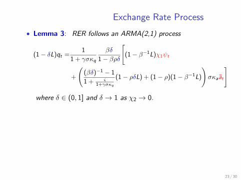
Exchange Rate Process

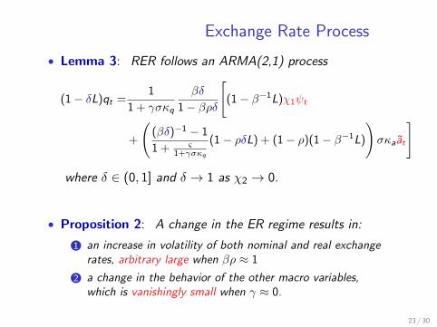
• Lemma 3: RER follows an ARMA(2,1) process

(1− δL)qt =1

1 + γσκq

βδ

1− βρδ

[(1− β−1L)χ1ψt

+

((βδ)−1 − 1

1 + ς1+γσκq

(1− ρδL) + (1− ρ)(1− β−1L)

)σκaat

]

where δ ∈ (0, 1] and δ → 1 as χ2 → 0.

• Proposition 2: A change in the ER regime results in:

1 an increase in volatility of both nominal and real exchangerates, arbitrary large when βρ ≈ 1

2 a change in the behavior of the other macro variables,which is vanishingly small when γ ≈ 0.

23 / 30

Exchange Rate Process

: IRF to ψt

0 4 8 12 16 20

-0.1

0

0.2

0.4

0.6

0.8

1

1.1

: IRF to at

0 4 8 12 16 20Quarters

-0.1

0

0.2

0.4

0.6

0.8

1

1.1

∆etet

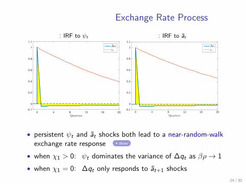
• persistent ψt and at shocks both lead to a near-random-walkexchange rate response show

• when χ1 > 0: ψt dominates the variance of ∆qt as βρ→ 1

• when χ1 = 0: ∆qt only responds to at+1 shocks

24 / 30

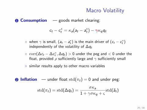
Macro Volatility

1 Consumption

— goods market clearing:

ct − c∗t = κa(at − a∗t )− γκqqt

◦ when γ is small, (at − a∗t ) is the main driver of (ct − c∗t )independently of the volatility of ∆qt

◦ corr(∆ct −∆c∗t ,∆qt) > 0 under the peg and < 0 under thefloat, provided ρ sufficiently large and γ sufficiently small

◦ similar results apply to other macro variables

2 Inflation

— under float std(πt) = 0 and under peg:

std(πt) = std(∆qt) =σκa

1 + γσκq + ςstd(at)

25 / 30

Macro Volatility

1 Consumption — goods market clearing:





2 Inflation

— under float std(πt) = 0 and under peg:



25 / 30

Macro Volatility

1 Consumption — goods market clearing:





2 Inflation — under float std(πt) = 0 and under peg:



25 / 30

Additional Evidence‘Overidentification’

1 Forward premium puzzle

• UIP and CIP both hold under peg (Frankel and Levich 1975)

• Forward Premium puzzle under float (Colacito and Croce 2013)

2 Backus-Smith puzzle show

• corr(∆q,∆c−∆c∗) switches sign: + under peg, − under float

(Colacito and Croce 2013, Devereux and Hnatkovska 2014)

3 Balassa-Samuelson effect

• holds no explanatory power under float (Engel 1999)

• works well under peg (Berka, Devereux and Engel 2018)

26 / 30

QUANTITATIVE EVALUATION

27 / 30

Quantitative Framework

• Sticky wages and LCP sticky prices (on/off)

• Taylor rule with a weight on nominal exchange rate

— ER regime calibrated to change std(∆et) eightfold

• Pricing-to-market and intermediate inputs

• Capital with adjustment costs

• Shocks:

1 Productivity or monetary shocks

2 Taste shock ξt

3 Financial shock ψt

• Standard calibration show

27 / 30

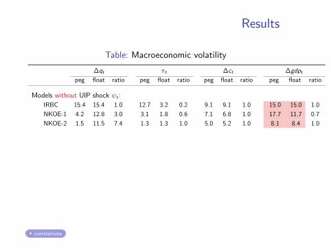
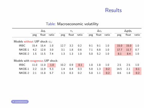
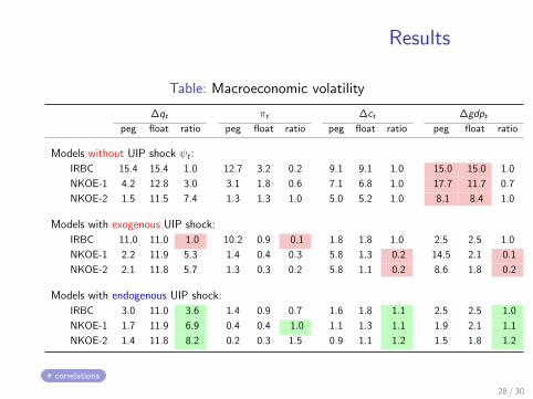
Results

Table: Macroeconomic volatility

∆qt πt ∆ct ∆gdpt

peg float ratio peg float ratio peg float ratio peg float ratio

Models without UIP shock ψt :

IRBC 15.4 15.4 1.0 12.7 3.2 0.2 9.1 9.1 1.0 15.0 15.0 1.0

NKOE-1 4.2 12.8 3.0 3.1 1.8 0.6 7.1 6.8 1.0 17.7 11.7 0.7

NKOE-2 1.5 11.5 7.4 1.3 1.3 1.0 5.0 5.2 1.0 8.1 8.4 1.0

Models with exogenous UIP shock:

IRBC 11.0 11.0 1.0 10.2 0.9 0.1 1.8 1.8 1.0 2.5 2.5 1.0

NKOE-1 2.2 11.9 5.3 1.4 0.4 0.3 5.8 1.3 0.2 14.5 2.1 0.1

NKOE-2 2.1 11.8 5.7 1.3 0.3 0.2 5.8 1.1 0.2 8.6 1.8 0.2

Models with endogenous UIP shock:

IRBC 3.0 11.0 3.6 1.4 0.9 0.7 1.6 1.8 1.1 2.5 2.5 1.0

NKOE-1 1.7 11.9 6.9 0.4 0.4 1.0 1.1 1.3 1.1 1.9 2.1 1.1

NKOE-2 1.4 11.8 8.2 0.2 0.3 1.5 0.9 1.1 1.2 1.5 1.8 1.2

correlations

28 / 30

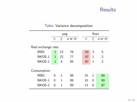
Results

Table: Variance decomposition

peg float

ψ ξ a or m ψ ξ a or m

Real exchange rate:

IRBC 1 23 76 92 3 5

NKOE-1 1 22 77 97 1 2

NKOE-2 1 4 95 97 1 2

Consumption:

IRBC 0 1 99 15 1 84

NKOE-1 0 1 99 10 0 90

NKOE-2 0 1 99 13 0 87

29 / 30

Conclusion

• Mussa facts are some of the most prominent pieces ofevidence of monetary non-neutrality

• We argue, however, that it is not directly suggestive ofnominal rigidities

— a weak test of nominal rigidities (and monetary vs productivityshocks), as it rejects both types of ‘conventional’ models

• Yet, it is highly suggestive of an alternative source ofnon-neutrality arising via the financial market

— a particular type of financial friction

— namely, segmented financial market, whereby nominalexchange rate risk is held in a concentrated way

• Important for reassessing the argument in favor of peg/float

30 / 30

APPENDIX

31 / 30

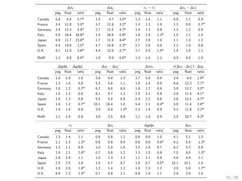
∆et ∆qt πt − π∗t ∆ct −∆c∗tpeg float ratio peg float ratio peg float ratio peg float ratio

Canada 0.8 4.4 5.7* 1.5 4.7 3.0* 1.3 1.4 1.1 0.8 1.1 0.9

France 3.4 11.8 3.5* 3.7 11.8 3.2* 1.3 1.3 1.0 1.2 0.9 0.7*

Germany 2.4 12.3 5.0* 2.7 12.5 4.7* 1.4 1.3 0.9 1.3 1.2 0.9

Italy 0.5 10.4 18.8* 1.5 10.4 6.9* 1.4 1.9 1.3* 1.0 1.1 1.0

Japan 0.8 11.7 13.8* 2.7 11.9 4.4* 2.7 2.8 1.0 1.1 1.3 1.2

Spain 4.4 10.8 2.5* 4.7 10.8 2.3* 2.7 2.6 0.9 1.2 1.0 0.8

U.K. 4.1 11.5 2.8* 4.4 12.0 2.7* 1.7 2.5 1.5* 1.4 1.5 1.1

RoW 1.2 9.8 8.0* 1.8 9.9 5.6* 1.3 1.4 1.1 0.9 0.9 1.0

∆gdpt −∆gdp∗t ∆yt −∆y∗t ∆nxt σ(∆ct−∆c∗t )−∆qt


Canada 1.0 1.0 1.0 3.8 4.9 1.3 1.7 1.6 0.9 2.4 4.5 1.9*

France 1.2 1.0 0.8 5.3 5.6 1.1 1.5 1.4 0.9 4.4 12.2 2.7*

Germany 1.8 1.2 0.7* 6.7 6.0 0.9 1.8 1.7 0.9 3.9 13.7 3.5*

Italy 1.5 1.3 0.8 8.1 9.7 1.2 2.5 2.2 0.9 2.8 11.4 4.1*

Japan 1.5 1.3 0.8 5.5 5.0 0.9 2.4 2.2 0.9 2.8 13.1 4.7*

Spain 1.6 1.2 0.7* 10.1 10.4 1.0 5.4 2.1 0.4* 5.8 11.4 2.0*

U.K. 1.4 1.4 0.9 3.9 6.0 1.5* 2.2 1.9 0.9 5.2 11.8 2.2*

RoW 1.1 1.0 0.8 3.9 3.5 0.9 1.1 1.0 0.9 2.5 10.7 4.3*

πt ∆ct ∆gdpt ∆yt


Canada 1.3 1.4 1.1 0.8 0.9 1.1 0.9 0.9 1.0 4.1 5.1 1.2

France 1.1 1.3 1.2* 0.9 0.8 0.9 0.9 0.6 0.6* 4.2 5.4 1.3*

Germany 1.2 1.1 0.9 1.0 1.0 1.0 1.5 1.0 0.7 6.2 5.7 0.9

Italy 1.0 2.1 2.0* 0.7 0.8 1.2 1.3 1.0 0.8 7.5 9.5 1.3*

Japan 2.6 2.9 1.1 1.0 1.3 1.3 1.1 1.1 0.9 4.6 4.9 1.1

Spain 2.5 2.5 1.0 1.0 0.7 0.7 1.4 0.7 0.5* 10.1 10.1 1.0

U.K. 1.6 2.6 1.6* 1.2 1.4 1.2 1.0 1.3 1.2 3.5 5.9 1.7*

U.S. 0.9 1.3 1.5* 0.7 0.8 1.1 0.9 1.0 1.1 2.9 2.9 1.032 / 30

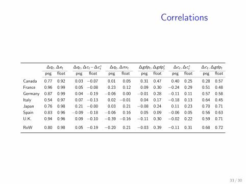
Correlations

∆qt ,∆et ∆qt ,∆ct−∆c∗t ∆qt ,∆nxt ∆gdpt ,∆gdp∗t ∆ct ,∆c∗t ∆ct ,∆gdpt

peg float peg float peg float peg float peg float peg float

Canada 0.77 0.92 0.03 −0.07 0.01 0.05 0.31 0.47 0.40 0.25 0.28 0.57

France 0.96 0.99 0.05 −0.08 0.23 0.12 0.09 0.30 −0.24 0.29 0.51 0.48

Germany 0.87 0.99 0.04 −0.19 −0.06 0.00 −0.01 0.28 −0.11 0.11 0.57 0.58

Italy 0.54 0.97 0.07 −0.13 0.02 −0.01 0.04 0.17 −0.18 0.13 0.64 0.45

Japan 0.76 0.98 0.21 −0.00 0.03 0.21 −0.08 0.24 0.11 0.23 0.70 0.71

Spain 0.83 0.96 −0.09 −0.18 −0.06 0.16 0.05 0.09 −0.06 0.05 0.56 0.63

U.K. 0.94 0.96 0.09 −0.10 −0.39 −0.16 −0.11 0.30 −0.02 0.22 0.59 0.71

RoW 0.80 0.98 0.05 −0.19 −0.20 0.21 −0.03 0.39 −0.11 0.31 0.68 0.72

33 / 30

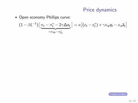
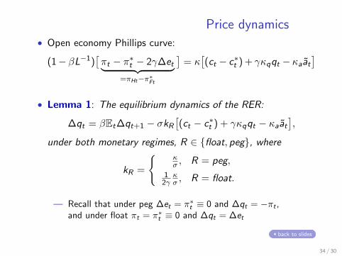
Price dynamics• Open economy Phillips curve:

(1− βL−1)[πt − π∗t − 2γ∆et︸︷︷︸

=πHt−π∗Ft

]= κ


]

• Lemma 1: The equilibrium dynamics of the RER:

∆qt = βEt∆qt+1 − σkR[(ct − c∗t ) + γκqqt − κaat

],

under both monetary regimes, R ∈ {float, peg}, where

kR =

{κσ , R = peg,

12γ

κσ , R = float.

— Recall that under peg ∆et = π∗t ≡ 0 and ∆qt = −πt ,and under float πt = π∗t ≡ 0 and ∆qt = ∆et

back to slides

34 / 30

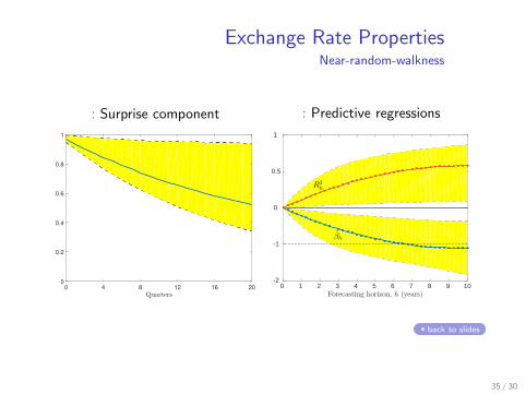
Exchange Rate PropertiesNear-random-walkness

: Surprise component

0 4 8 12 16 20

0

0.2

0.4

0.6

0.8

1

: Predictive regressions

0 1 2 3 4 5 6 7 8 9 10Forecasting horizon, h (years)

-2

-1

0

0.5

1

R2h

βh

back to slides

35 / 30

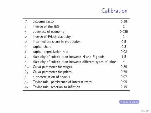
Calibration

β discount factor 0.99

σ inverse of the IES 2

γ openness of economy 0.035

ϕ inverse of Frisch elasticity 1

φ intermediate share in production 0.5

ϑ capital share 0.3

δ capital depreciation rate 0.02

θ elasticity of substitution between H and F goods 1.5

ε elasticity of substitution between different types of labor 4

λw Calvo parameter for wages 0.85

λp Calvo parameter for prices 0.75

ρ autocorrelation of shocks 0.97

ρr Taylor rule: persistence of interest rates 0.95

φπ Taylor rule: reaction to inflation 2.15

back to slides

36 / 30

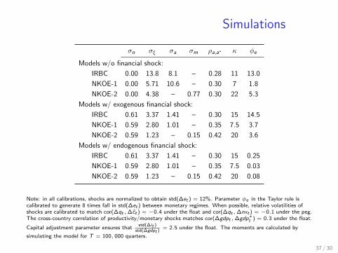
Simulations

σn σξ σa σm ρa,a∗ κ φe

Models w/o financial shock:

IRBC 0.00 13.8 8.1 – 0.28 11 13.0

NKOE-1 0.00 5.71 10.6 – 0.30 7 1.8

NKOE-2 0.00 4.38 – 0.77 0.30 22 5.3

Models w/ exogenous financial shock:

IRBC 0.61 3.37 1.41 – 0.30 15 14.5

NKOE-1 0.59 2.80 1.01 – 0.35 7.5 3.7

NKOE-2 0.59 1.23 – 0.15 0.42 20 3.6

Models w/ endogenous financial shock:

IRBC 0.61 3.37 1.41 – 0.30 15 0.25

NKOE-1 0.59 2.80 1.01 – 0.35 7.5 0.03

NKOE-2 0.59 1.23 – 0.15 0.42 20 0.08

Note: in all calibrations, shocks are normalized to obtain std(∆et ) = 12%. Parameter φe in the Taylor rule iscalibrated to generate 8 times fall in std(∆et ) between monetary regimes. When possible, relative volatilities ofshocks are calibrated to match cor(∆qt ,∆ct ) = −0.4 under the float and cor(∆qt ,∆nxt ) = −0.1 under the peg.The cross-country correlation of productivity/monetary shocks matches cor(∆gdpt ,∆gdp∗t ) = 0.3 under the float.

Capital adjustment parameter ensures thatstd(∆it )

std(∆gdpt )= 2.5 under the float. The moments are calculated by

simulating the model for T = 100, 000 quarters.

37 / 30

Simulated Correlations

Panel B: correlations

∆qt ,∆et ∆qt ,∆ct−∆c∗t ∆qt ,∆nxt ∆gdpt ,∆gdp∗t ∆ct ,∆c∗t ∆ct ,∆gdpt βUIP

peg float peg float peg float peg float peg float peg float peg float

Models w/o financial shock:

IRBC 0.86 0.99 0.91 0.91 −0.10 −0.10 0.30 0.30 0.34 0.34 0.99 0.99 0.8 0.9

NKOE-1 0.67 0.99 0.28 0.70 −0.10 −0.49 0.38 0.31 0.65 0.41 0.91 0.97 0.3 1.0

NKOE-2 0.96 0.99 0.49 0.99 −0.10 0.05 0.95 0.30 0.97 0.33 1.00 1.00 1.0 1.0

Models w/ exogenous financial shock:

IRBC 0.86 0.99 −0.40 −0.40 0.93 0.93 0.30 0.30 0.15 0.15 0.88 0.88 0.0 −1.3

NKOE-1 0.81 1.00 −0.88 −0.40 0.89 0.93 0.60 0.30 −0.06 0.32 0.99 0.84 −0.1 −1.6

NKOE-2 0.82 1.00 −0.89 −0.40 0.92 0.97 0.51 0.30 −0.10 0.26 1.00 0.79 −0.1 −2.2

Models w/ endogenous financial shock:

IRBC 0.98 1.00 0.92 −0.40 −0.10 0.93 0.30 0.30 0.39 0.16 0.99 0.88 1.0 −1.4

NKOE-1 0.98 1.00 0.84 −0.40 −0.10 0.93 0.44 0.30 0.54 0.32 0.96 0.84 1.0 −1.6

NKOE-2 1.00 1.00 0.94 −0.40 −0.10 0.97 0.66 0.30 0.70 0.26 0.99 0.79 1.0 −2.3

back to slides

38 / 30

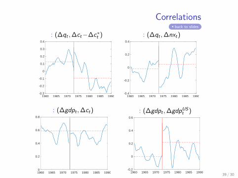
Correlationsback to slides

: (∆qt ,∆ct−∆c∗t )

1960 1965 1970 1975 1980 1985 1990-0.3

-0.2

-0.1

0

0.1

0.2

0.3

0.4

: (∆qt ,∆nxt)

1960 1965 1970 1975 1980 1985 1990-0.4

-0.2

0

0.2

0.4

: (∆gdpt ,∆ct)

1960 1965 1970 1975 1980 1985 19900

0.2

0.4

0.6

0.8

: (∆gdpt ,∆gdpUSt )

1960 1965 1970 1975 1980 1985 1990-0.2

0

0.2

0.4

0.6

39 / 30

Model Setup III• Fiscal authority:

Tt =∑

j∈Jt−1

(1− e−ζ

jt)D j

tBjt

• Monetary authority:

it = ρmit−1 + (1− ρm)[φππt + φe(et − e)

]+ σmε

mt

— limiting case: (i) φπ→∞ ⇒ πt≡0 or (ii) φe→∞ ⇒ ∆et≡0

• Market clearing in labor and product market:

Lt = e−at∫ 1

0Yt(i)di and CHt(i) + C∗Ht(i) = Yt(i)

and financial market:

B jt+1 + B j∗

t+1 = 0 ∀j ∈ Jt ∩ J∗t given price Θjt

40 / 30

Mussa Puzzle Redux - Princeton University

Documents

Transcript of Mussa Puzzle Redux - Princeton University