Multi-Step Forecast Variancessc.wisc.edu/~bhansen/460/460Lecture12 2017.pdfMulti-Step Forecast...
46
Multi-Step Forecast Variance • Can use plug-in, iterated, or direct method • Easiest method is direct • Forecast variance can be computed from direct regression t h t t u y y ˆ ˆ ˆ * * + + = − β α ∑ = = T t t u u T 1 2 2 ˆ 1 ˆ σ
Transcript of Multi-Step Forecast Variancessc.wisc.edu/~bhansen/460/460Lecture12 2017.pdfMulti-Step Forecast...
Multi-Step Forecast Variance
• Can use plug-in, iterated, or direct method• Easiest method is direct• Forecast variance can be computed from
direct regression
thtt uyy ˆˆˆ ** ++= −βα
∑=
=T
ttu u
T 1
22 ˆ1σ̂
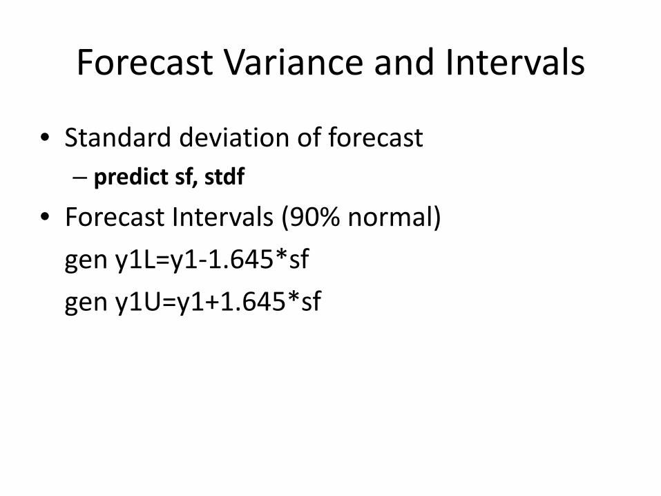
Forecast Variance and Intervals
• Standard deviation of forecast– predict sf, stdf
• Forecast Intervals (90% normal)gen y1L=y1-1.645*sfgen y1U=y1+1.645*sf
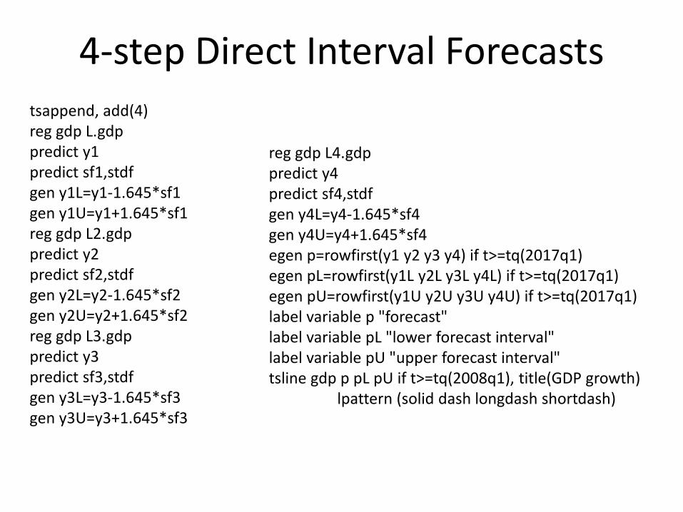
4-step Direct Interval Forecaststsappend, add(4)reg gdp L.gdppredict y1predict sf1,stdfgen y1L=y1-1.645*sf1gen y1U=y1+1.645*sf1reg gdp L2.gdppredict y2predict sf2,stdfgen y2L=y2-1.645*sf2gen y2U=y2+1.645*sf2reg gdp L3.gdppredict y3predict sf3,stdfgen y3L=y3-1.645*sf3gen y3U=y3+1.645*sf3
reg gdp L4.gdppredict y4predict sf4,stdfgen y4L=y4-1.645*sf4gen y4U=y4+1.645*sf4egen p=rowfirst(y1 y2 y3 y4) if t>=tq(2017q1)egen pL=rowfirst(y1L y2L y3L y4L) if t>=tq(2017q1)egen pU=rowfirst(y1U y2U y3U y4U) if t>=tq(2017q1)label variable p "forecast"label variable pL "lower forecast interval"label variable pU "upper forecast interval"tsline gdp p pL pU if t>=tq(2008q1), title(GDP growth)
lpattern (solid dash longdash shortdash)
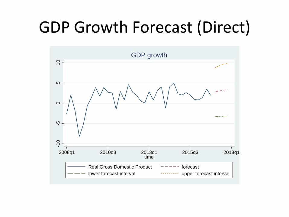
GDP Growth Forecast (Direct)-1
0-5
05
10
2008q1 2010q3 2013q1 2015q3 2018q1time
Real Gross Domestic Product forecastlower forecast interval upper forecast interval
GDP growth
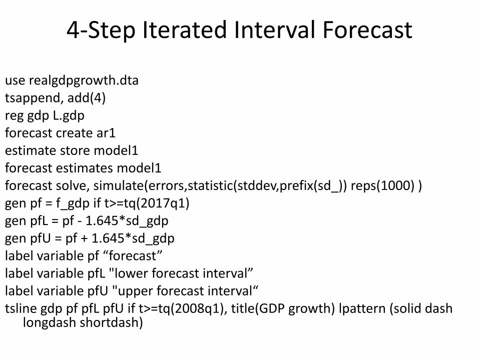
4-Step Iterated Interval Forecast
use realgdpgrowth.dtatsappend, add(4)reg gdp L.gdpforecast create ar1estimate store model1forecast estimates model1forecast solve, simulate(errors,statistic(stddev,prefix(sd_)) reps(1000) )gen pf = f_gdp if t>=tq(2017q1)gen pfL = pf - 1.645*sd_gdpgen pfU = pf + 1.645*sd_gdplabel variable pf “forecast”label variable pfL "lower forecast interval”label variable pfU "upper forecast interval“tsline gdp pf pfL pfU if t>=tq(2008q1), title(GDP growth) lpattern (solid dash
longdash shortdash)
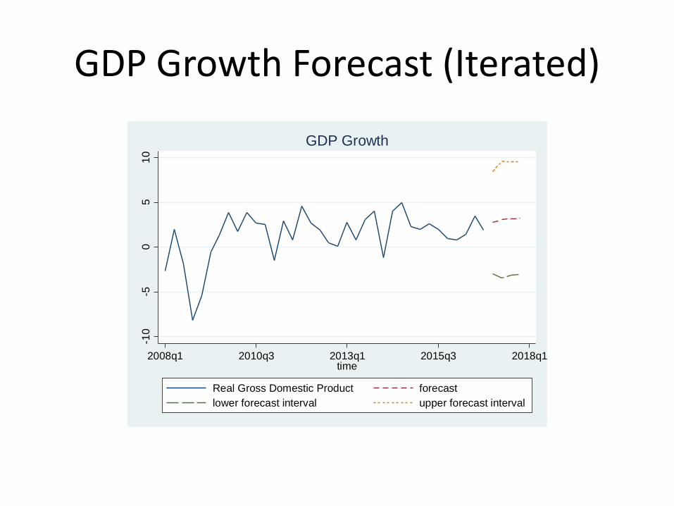
GDP Growth Forecast (Iterated)
-10
-50
510
2008q1 2010q3 2013q1 2015q3 2018q1time
Real Gross Domestic Product forecastlower forecast interval upper forecast interval
GDP Growth
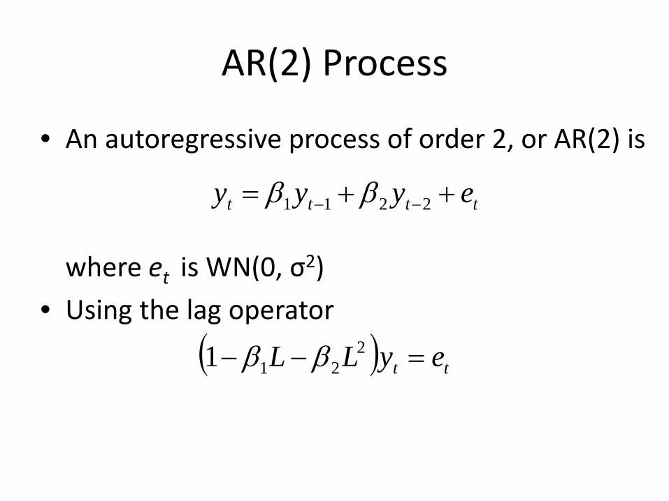
AR(2) Process
• An autoregressive process of order 2, or AR(2) is
where et is WN(0, σ2) • Using the lag operator
tttt eyyy ++= −− 2211 ββ
( ) tt eyLL =−− 2211 ββ
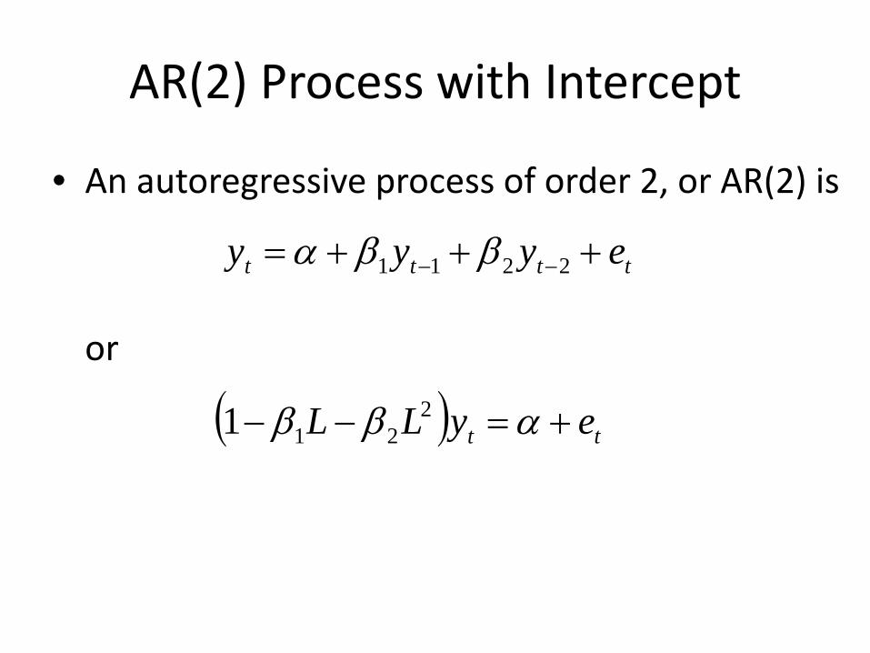
AR(2) Process with Intercept
• An autoregressive process of order 2, or AR(2) is
or
tttt eyyy +++= −− 2211 ββα
( ) tt eyLL +=−− αββ 2211
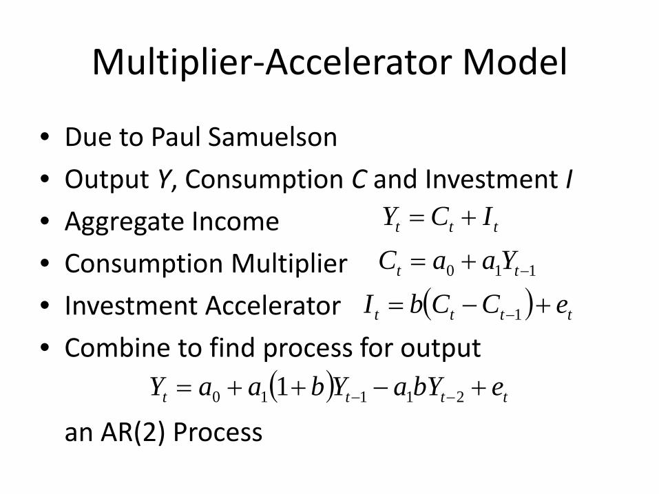
Multiplier-Accelerator Model
• Due to Paul Samuelson• Output Y, Consumption C and Investment I• Aggregate Income• Consumption Multiplier• Investment Accelerator• Combine to find process for output
an AR(2) Process
ttt ICY +=
110 −+= tt YaaC( ) tttt eCCbI +−= −1
( ) tttt ebYaYbaaY +−++= −− 21110 1
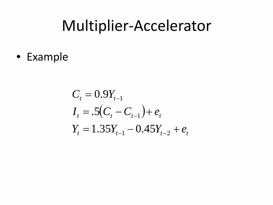
Multiplier-Accelerator
• Example
( )tttt
tttt
tt
eYYYeCCI
YC
+−=+−=
=
−−
−
−
21
1
1
45.035.15.
9.0

Simulated Example-2
-10
12
e
0 20 40 60 80 100t
White Noise
-10
-50
5y
0 20 40 60 80 100t
AR(2)
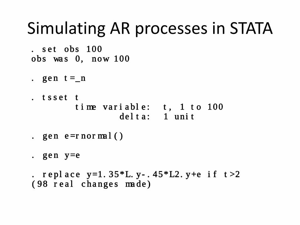
Simulating AR processes in STATA
(98 real changes made). replace y=1.35*L.y-.45*L2.y+e if t>2
. gen y=e
. gen e=rnormal()
delta: 1 unit time variable: t, 1 to 100. tsset t
. gen t=_n
obs was 0, now 100. set obs 100
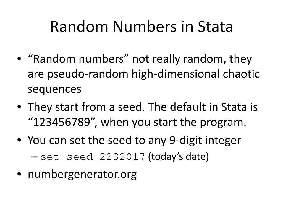
Random Numbers in Stata
• “Random numbers” not really random, they are pseudo-random high-dimensional chaotic sequences
• They start from a seed. The default in Stata is “123456789”, when you start the program.
• You can set the seed to any 9-digit integer– set seed 2232017 (today’s date)
• numbergenerator.org
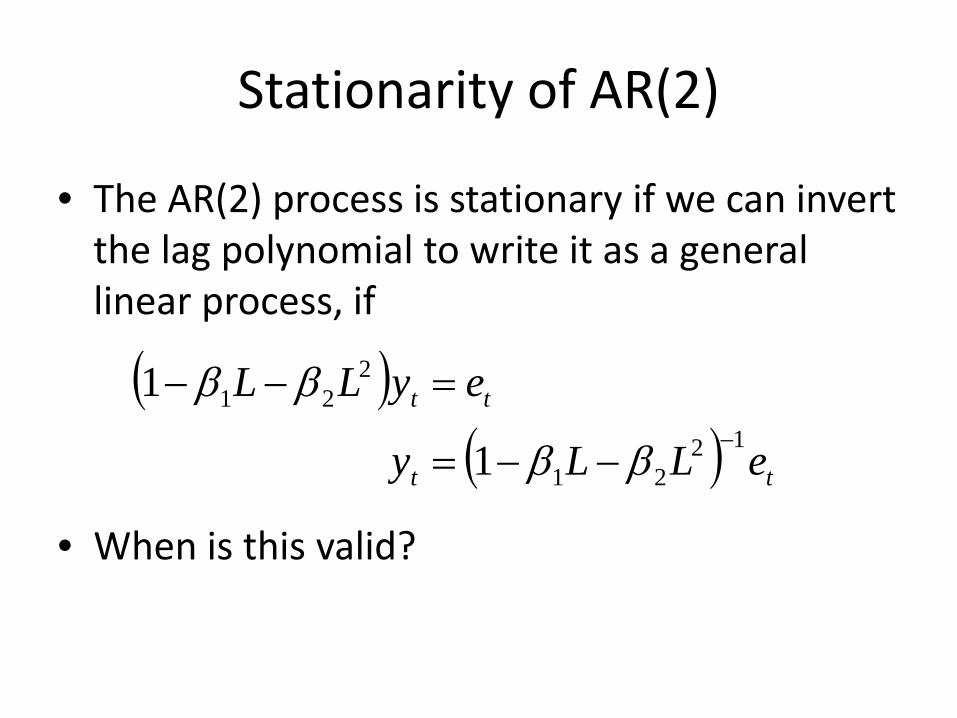
Stationarity of AR(2)
• The AR(2) process is stationary if we can invert the lag polynomial to write it as a general linear process, if
• When is this valid?
( )( ) tt
tt
eLLy
eyLL12
21
221
1
1−
−−=
=−−
ββ
ββ
Factors
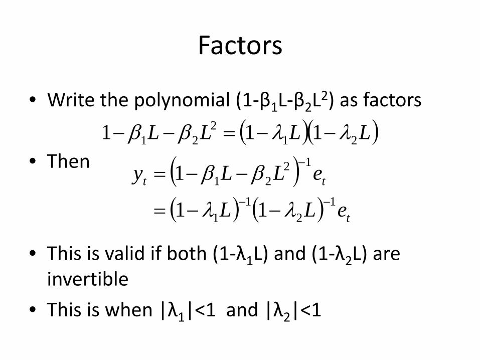
• Write the polynomial (1-β1L-β2L2) as factors
• Then
• This is valid if both (1-λ1L) and (1-λ2L) are invertible
• This is when |λ1|<1 and |λ2|<1
( )( )LLLL 212
21 111 λλββ −−=−−
( )( ) ( ) t
tt
eLL
eLLy1
21
1
1221
11
1−−
−
−−=
−−=
λλ
ββ
Stationary Roots
• λ1 and λ2 are the inverses of the roots of the polynomial (1-β1L-β2L2)
• They can be real or complex• If |λ1|<1 and |λ2|<1 we say they “are within
the unit circle”• The AR(2) is stationary if the inverse roots are
within the unit circle (are less than one in absolute value)
Necessary Condition
• The polynomial (1-β1L-β2L2) has a unit root if it equals 0 when L=1
• In this case, 1-β1-β2=0• Or β1+β2=1• This means that the AR(2) is nonstationary if
the sum of the AR coefficients equals 1
Multiplier Example
• In the model
the sum of the coefficients is a1, the consumption coefficient.
• In this model, if a1=1, then the output process has a unit root, it is nonstationary
( ) tttt ebYaYbaaY +−++= −− 21110 1
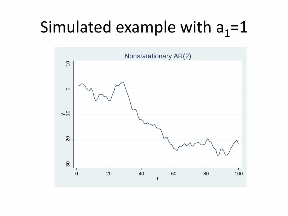
Simulated example with a1=1
-30
-20
-10
010
y
0 20 40 60 80 100t
Nonstatationary AR(2)
Autocorrelation of AR(2)
• The autocorrelations of an AR(2) can be much more complicated than that of an AR(1)
• Take the example
• Simulated a time series with T=500 observations from this example
• Calculated sample autocorrelation function
tttt eYYY +−= −− 21 9.05.1
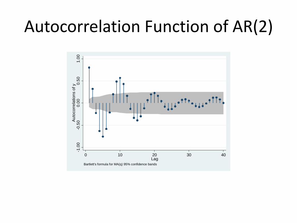
Autocorrelation Function of AR(2)
-1.0
0-0
.50
0.00
0.50
1.00
Auto
corre
latio
ns o
f y
0 10 20 30 40Lag
Bartlett's formula for MA(q) 95% confidence bands
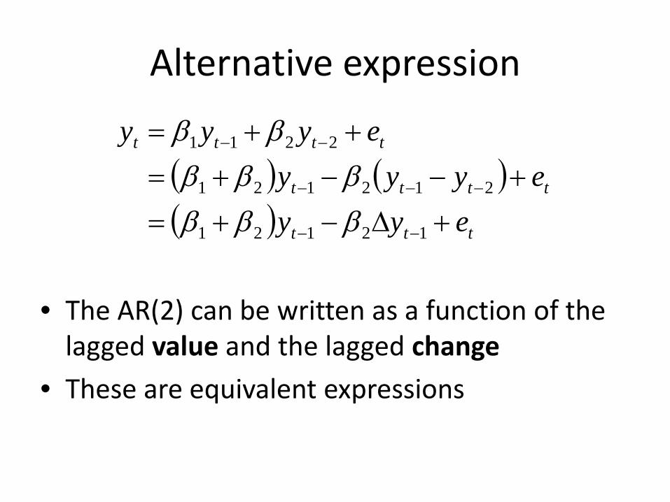
Alternative expression
• The AR(2) can be written as a function of the lagged value and the lagged change
• These are equivalent expressions
( ) ( )( ) ttt
tttt
tttt
eyyeyyy
eyyy
+∆−+=+−−+=
++=
−−
−−−
−−
12121
212121
2211
ββββββ
ββ
Estimation of AR(2)
• Least Squares Regression
tttt eyyy ˆˆˆˆ 2211 +++= −− ββα
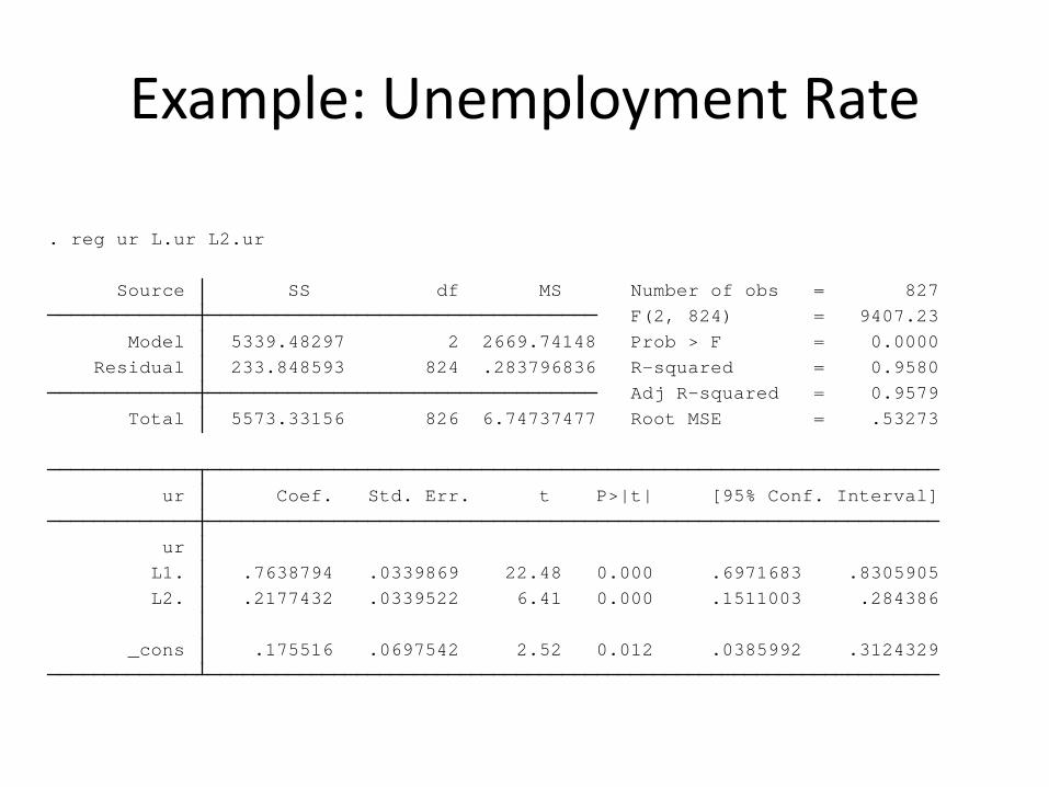
Example: Unemployment Rate
_cons .175516 .0697542 2.52 0.012 .0385992 .3124329 L2. .2177432 .0339522 6.41 0.000 .1511003 .284386 L1. .7638794 .0339869 22.48 0.000 .6971683 .8305905 ur ur Coef. Std. Err. t P>|t| [95% Conf. Interval]
Total 5573.33156 826 6.74737477 Root MSE = .53273 Adj R-squared = 0.9579 Residual 233.848593 824 .283796836 R-squared = 0.9580 Model 5339.48297 2 2669.74148 Prob > F = 0.0000 F(2, 824) = 9407.23 Source SS df MS Number of obs = 827
. reg ur L.ur L2.ur
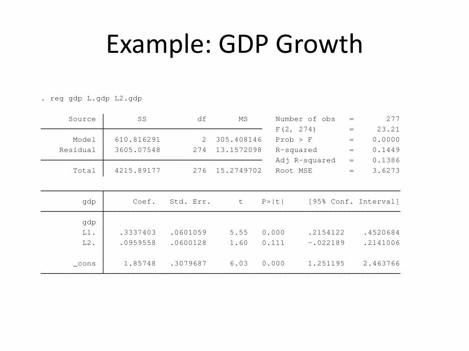
Example: GDP Growth
_cons 1.85748 .3079687 6.03 0.000 1.251195 2.463766 L2. .0959558 .0600128 1.60 0.111 -.022189 .2141006 L1. .3337403 .0601059 5.55 0.000 .2154122 .4520684 gdp gdp Coef. Std. Err. t P>|t| [95% Conf. Interval]
Total 4215.89177 276 15.2749702 Root MSE = 3.6273 Adj R-squared = 0.1386 Residual 3605.07548 274 13.1572098 R-squared = 0.1449 Model 610.816291 2 305.408146 Prob > F = 0.0000 F(2, 274) = 23.21 Source SS df MS Number of obs = 277
. reg gdp L.gdp L2.gdp
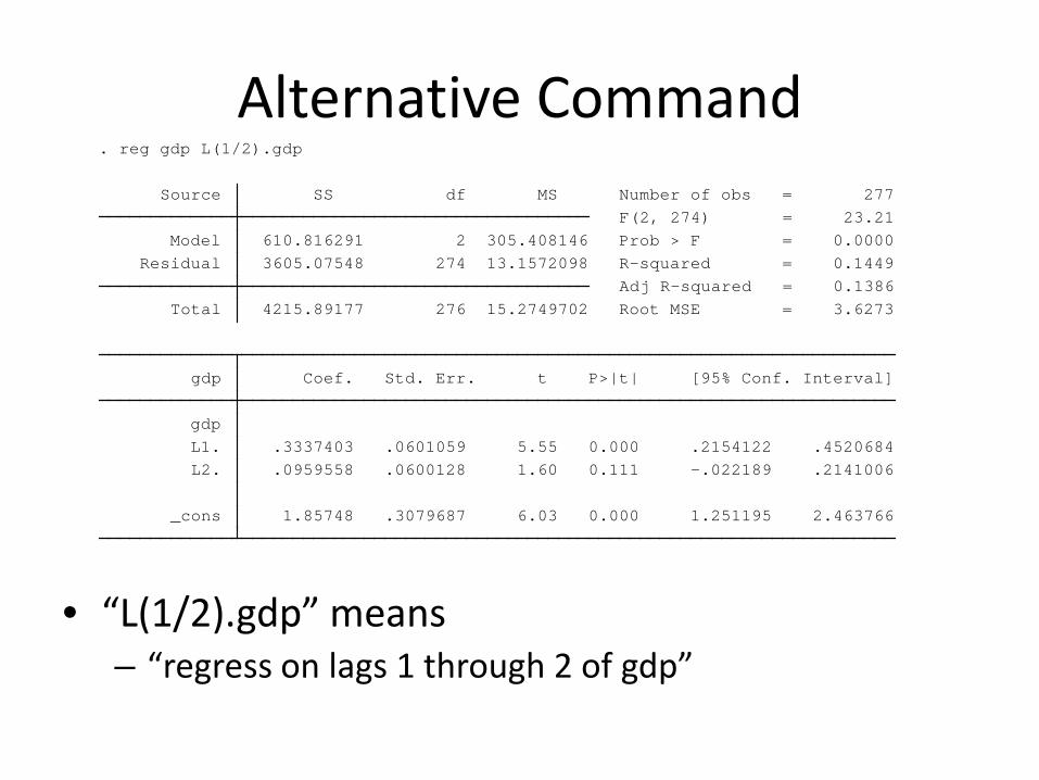
Alternative Command
• “L(1/2).gdp” means – “regress on lags 1 through 2 of gdp”
_cons 1.85748 .3079687 6.03 0.000 1.251195 2.463766 L2. .0959558 .0600128 1.60 0.111 -.022189 .2141006 L1. .3337403 .0601059 5.55 0.000 .2154122 .4520684 gdp gdp Coef. Std. Err. t P>|t| [95% Conf. Interval]
Total 4215.89177 276 15.2749702 Root MSE = 3.6273 Adj R-squared = 0.1386 Residual 3605.07548 274 13.1572098 R-squared = 0.1449 Model 610.816291 2 305.408146 Prob > F = 0.0000 F(2, 274) = 23.21 Source SS df MS Number of obs = 277
. reg gdp L(1/2).gdp
One-Step-Ahead Forecast
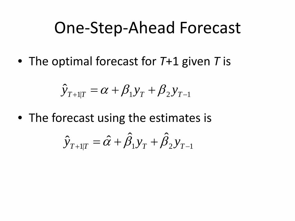
• The optimal forecast for T+1 given T is
• The forecast using the estimates is
121|1ˆ −+ ++= TTTT yyy ββα
121|1ˆˆˆˆ −+ ++= TTTT yyy ββα
Two-Step-Ahead Forecast
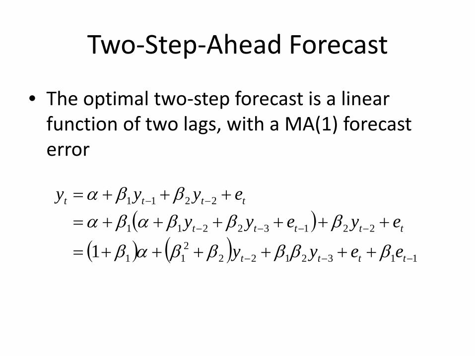
• The optimal two-step forecast is a linear function of two lags, with a MA(1) forecast error
( )( ) ( ) 1132122
211
22132211
2211
1 −−−
−−−−
−−
++++++=
++++++=+++=
tttt
ttttt
tttt
eeyyeyeyy
eyyy
βββββαβ
βββαβαββα
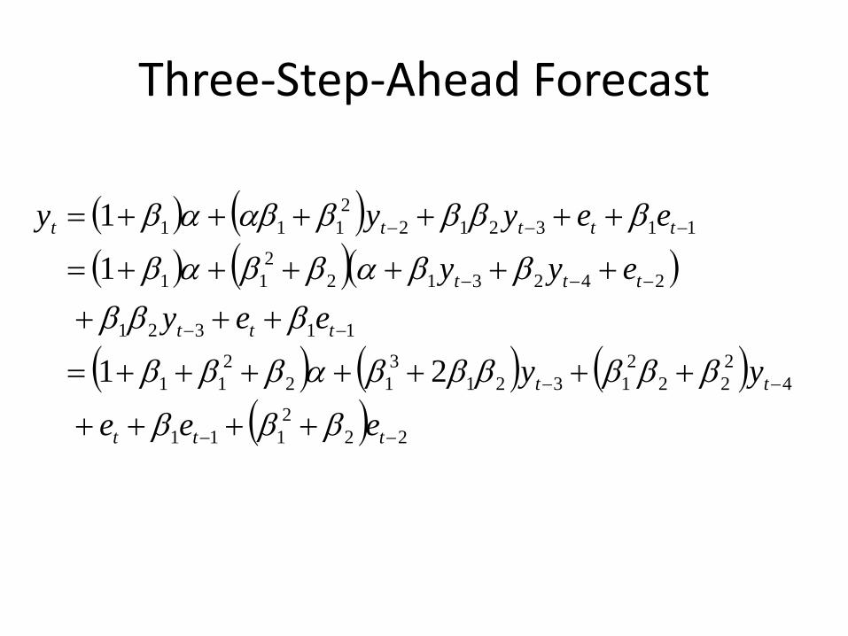
Three-Step-Ahead Forecast
( ) ( )( ) ( )( )
( ) ( ) ( )( ) 22
2111
4222
21321
312
211
11321
2423122
11
1132122
111
21
11
−−
−−
−−
−−−
−−−
++++
+++++++=
+++++++++=
++++++=
ttt
tt
ttt
ttt
ttttt
eeeyy
eeyeyy
eeyyy
βββ
ββββββαβββ
βββββαββαβ
ββββαβαβ
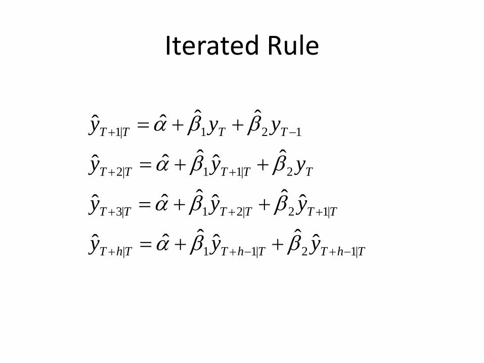
Iterated Rule
ThTThTThT
TTTTTT
TTTTT
TTTT
yyy
yyy
yyy
yyy
|12|11|
|12|21|3
2|11|2
121|1
ˆˆˆˆˆˆ
ˆˆˆˆˆˆ
ˆˆˆˆˆ
ˆˆˆˆ
−+−++
+++
++
−+
++=
++=
++=
++=
ββα
ββα
ββα
ββα
Direct Forecast
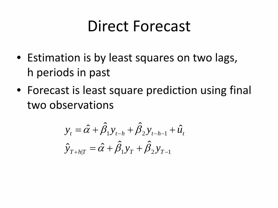
• Estimation is by least squares on two lags, h periods in past
• Forecast is least square prediction using final two observations
121|
121
ˆˆˆˆ
ˆˆˆˆ
−+
−−−
++=
+++=
TTThT
ththtt
yyy
uyyy
ββα
ββα
AR(p) Process
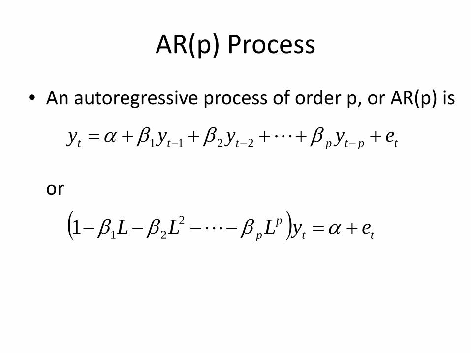
• An autoregressive process of order p, or AR(p) is
or
tptpttt eyyyy +++++= −−− βββα 2211
( ) ttp
p eyLLL +=−−−− αβββ 2211
Stationarity
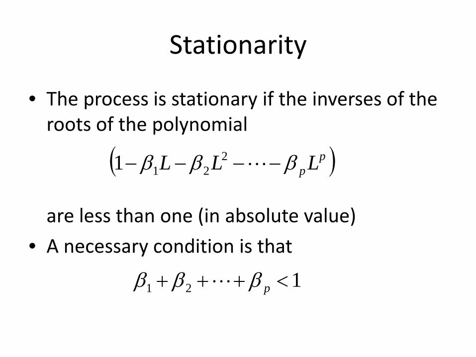
• The process is stationary if the inverses of the roots of the polynomial
are less than one (in absolute value)• A necessary condition is that
( )pp LLL βββ −−−− 2
211
121 <+++ pβββ
Alternative Representation
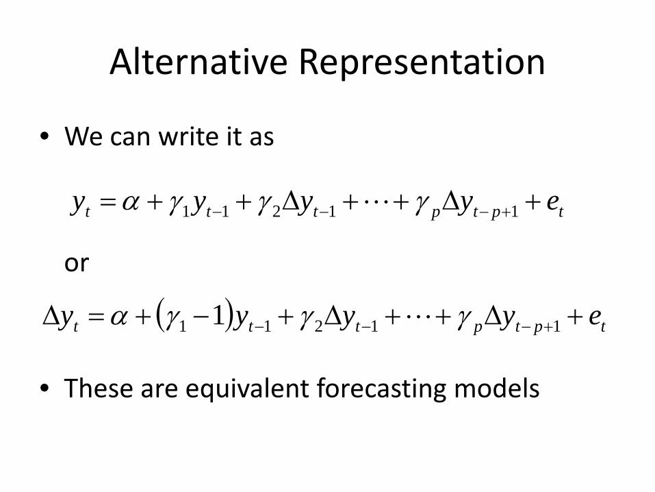
• We can write it as
or
• These are equivalent forecasting models
tptpttt eyyyy +∆++∆++= +−−− 11211 γγγα
( ) tptpttt eyyyy +∆++∆+−+=∆ +−−− 11211 1 γγγα
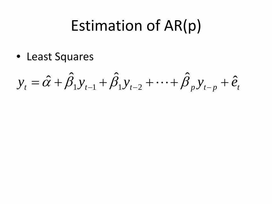
Estimation of AR(p)
• Least Squares
tptpttt eyyyy ˆˆˆˆˆ 2111 +++++= −−− βββα
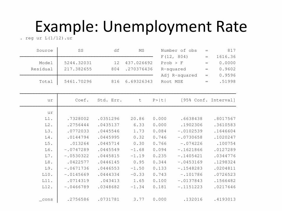
Example: Unemployment Rate
_cons .2756586 .0731781 3.77 0.000 .132016 .4193013 L12. -.0466789 .0348682 -1.34 0.181 -.1151223 .0217646 L11. .0714319 .043413 1.65 0.100 -.0137843 .1566482 L10. -.0145669 .0444334 -0.33 0.743 -.101786 .0726523 L9. -.0671736 .0446553 -1.50 0.133 -.1548283 .0204811 L8. .0422577 .0446145 0.95 0.344 -.0453169 .1298324 L7. -.0530322 .0445815 -1.19 0.235 -.1405421 .0344776 L6. -.0747289 .0445549 -1.68 0.094 -.1621866 .0127289 L5. .013264 .0445714 0.30 0.766 -.074226 .100754 L4. .0144794 .0445995 0.32 0.746 -.0730658 .1020247 L3. .0772033 .0445546 1.73 0.084 -.0102539 .1646604 L2. .2756444 .0435137 6.33 0.000 .1902306 .3610583 L1. .7328002 .0351296 20.86 0.000 .6638438 .8017567 ur ur Coef. Std. Err. t P>|t| [95% Conf. Interval]
Total 5461.70296 816 6.69326343 Root MSE = .51998 Adj R-squared = 0.9596 Residual 217.382655 804 .270376436 R-squared = 0.9602 Model 5244.32031 12 437.026692 Prob > F = 0.0000 F(12, 804) = 1616.36 Source SS df MS Number of obs = 817
. reg ur L(1/12).ur
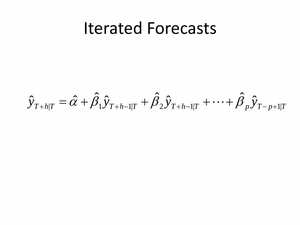
Iterated Forecasts
TpTpThTThTThT yyyy |1|12|11| ˆˆˆˆˆˆˆˆ +−−+−++ ++++= βββα
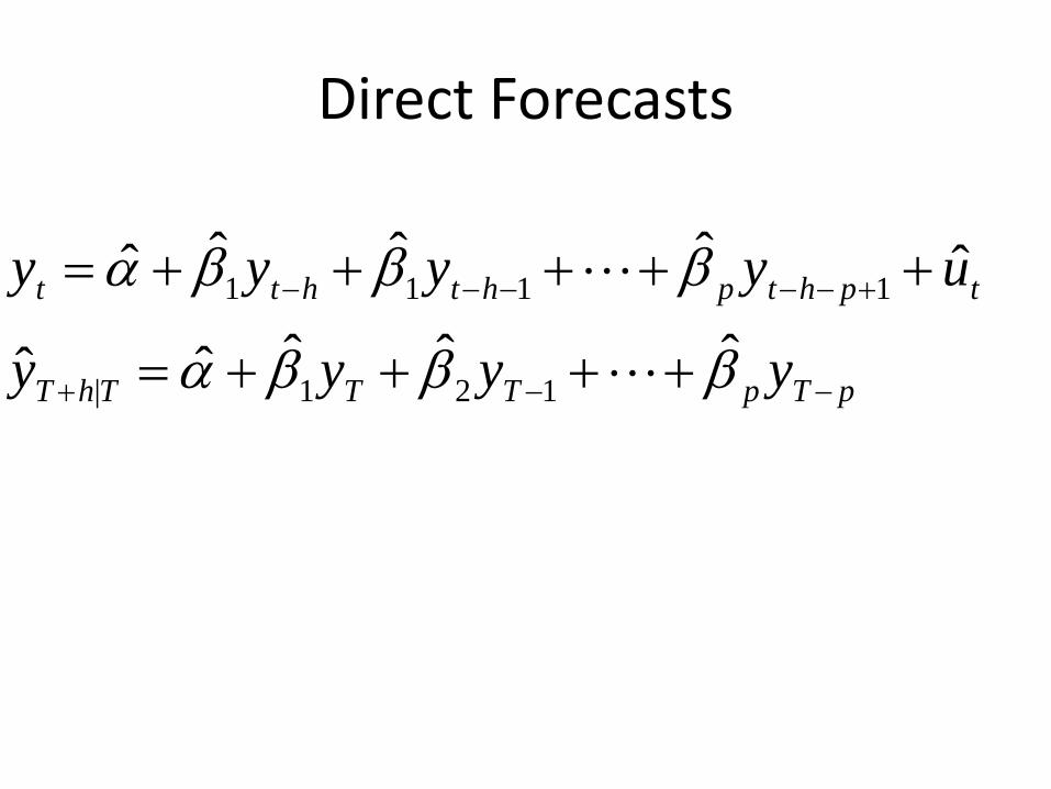
Direct Forecasts
pTpTTThT
tphtphthtt
yyyy
uyyyy
−−+
+−−−−−
++++=
+++++=
βββα
βββαˆˆˆˆˆ
ˆˆˆˆˆ
121|
1111
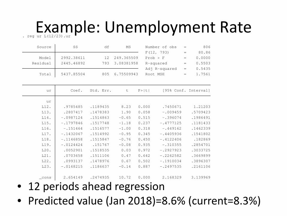
Example: Unemployment Rate
• 12 periods ahead regression• Predicted value (Jan 2018)=8.6% (current=8.3%)
_cons 2.654149 .2474935 10.72 0.000 2.168329 3.139969 L23. -.0168215 .1186637 -0.14 0.887 -.2497535 .2161106 L22. .0993137 .1478976 0.67 0.502 -.1910034 .3896307 L21. .0703658 .1511106 0.47 0.642 -.2262582 .3669899 L20. .0052901 .1518535 0.03 0.972 -.2927923 .3033725 L19. -.0124424 .151767 -0.08 0.935 -.310355 .2854701 L18. -.1146858 .1515847 -0.76 0.450 -.4122406 .182869 L17. -.1432067 .1514992 -0.95 0.345 -.4405936 .1541802 L16. -.151464 .1516577 -1.00 0.318 -.449162 .1462339 L15. -.1797846 .1517748 -1.18 0.237 -.4777125 .1181433 L14. -.0987124 .1514863 -0.65 0.515 -.396074 .1986491 L13. .2807417 .1478383 1.90 0.058 -.009459 .5709423 L12. .9785485 .1189435 8.23 0.000 .7450671 1.21203 ur ur Coef. Std. Err. t P>|t| [95% Conf. Interval]
Total 5437.85504 805 6.75509943 Root MSE = 1.7561 Adj R-squared = 0.5435 Residual 2445.46892 793 3.08381958 R-squared = 0.5503 Model 2992.38611 12 249.365509 Prob > F = 0.0000 F(12, 793) = 80.86 Source SS df MS Number of obs = 806
. reg ur L(12/23).ur
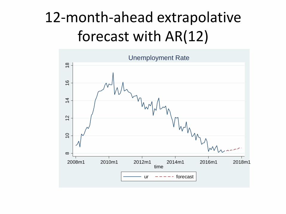
12-month-ahead extrapolative forecast with AR(12)
810
1214
1618
2008m1 2010m1 2012m1 2014m1 2016m1 2018m1time
ur forecast
Unemployment Rate
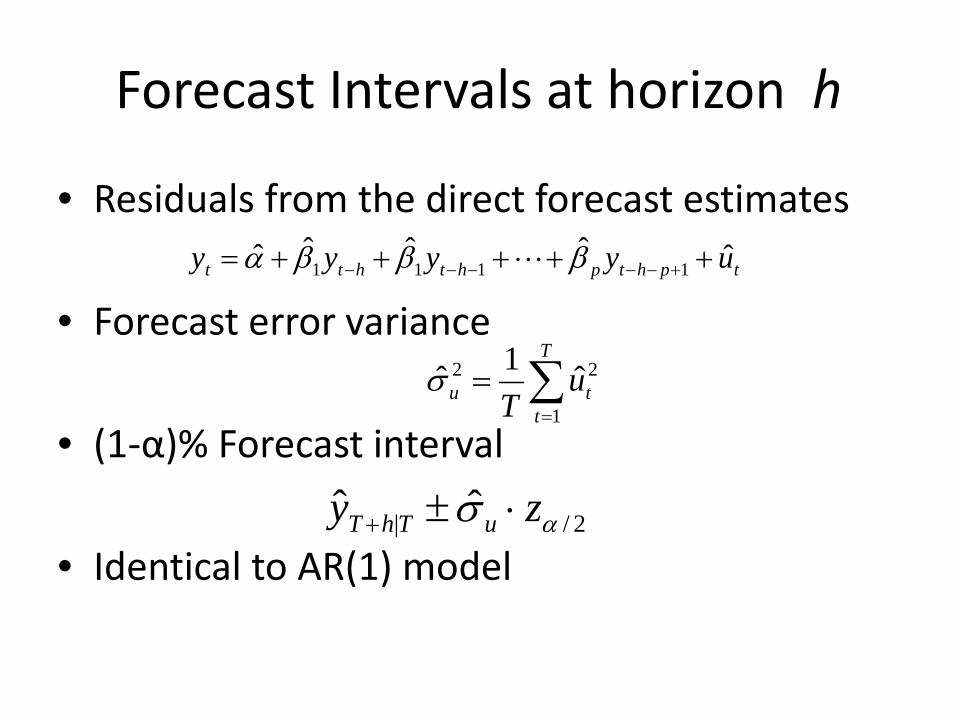
Forecast Intervals at horizon h
• Residuals from the direct forecast estimates
• Forecast error variance
• (1-α)% Forecast interval
• Identical to AR(1) model
tphtphthtt uyyyy ˆˆˆˆˆ 1111 +++++= +−−−−− βββα
∑=
=T
ttu u
T 1
22 ˆ1σ̂
2/| ˆˆ ασ zy uThT ⋅±+
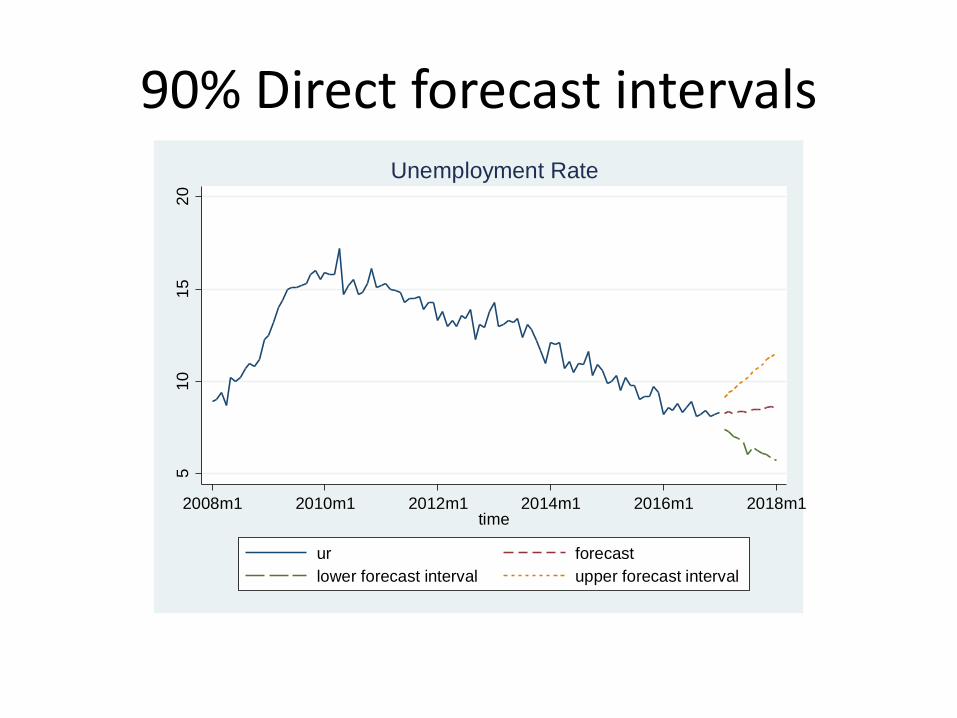
90% Direct forecast intervals5
1015
20
2008m1 2010m1 2012m1 2014m1 2016m1 2018m1time
ur forecastlower forecast interval upper forecast interval
Unemployment Rate
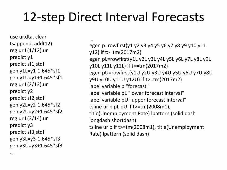
12-step Direct Interval Forecastsuse ur.dta, cleartsappend, add(12)reg ur L(1/12).urpredict y1predict sf1,stdfgen y1L=y1-1.645*sf1gen y1U=y1+1.645*sf1reg ur L(2/13).urpredict y2predict sf2,stdfgen y2L=y2-1.645*sf2gen y2U=y2+1.645*sf2reg ur L(3/14).urpredict y3predict sf3,stdfgen y3L=y3-1.645*sf3gen y3U=y3+1.645*sf3…
…egen p=rowfirst(y1 y2 y3 y4 y5 y6 y7 y8 y9 y10 y11 y12) if t>=tm(2017m2)egen pL=rowfirst(y1L y2L y3L y4L y5L y6L y7L y8L y9L y10L y11L y12L) if t>=tm(2017m2)egen pU=rowfirst(y1U y2U y3U y4U y5U y6U y7U y8U y9U y10U y11U y12U) if t>=tm(2017m2)label variable p "forecast"label variable pL "lower forecast interval"label variable pU "upper forecast interval"tsline ur p pL pU if t>=tm(2008m1), title(Unemployment Rate) lpattern (solid dash longdash shortdash)tsline ur p if t>=tm(2008m1), title(Unemployment Rate) lpattern (solid dash)
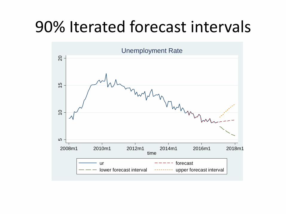
90% Iterated forecast intervals
510
1520
2008m1 2010m1 2012m1 2014m1 2016m1 2018m1time
ur forecastlower forecast interval upper forecast interval
Unemployment Rate
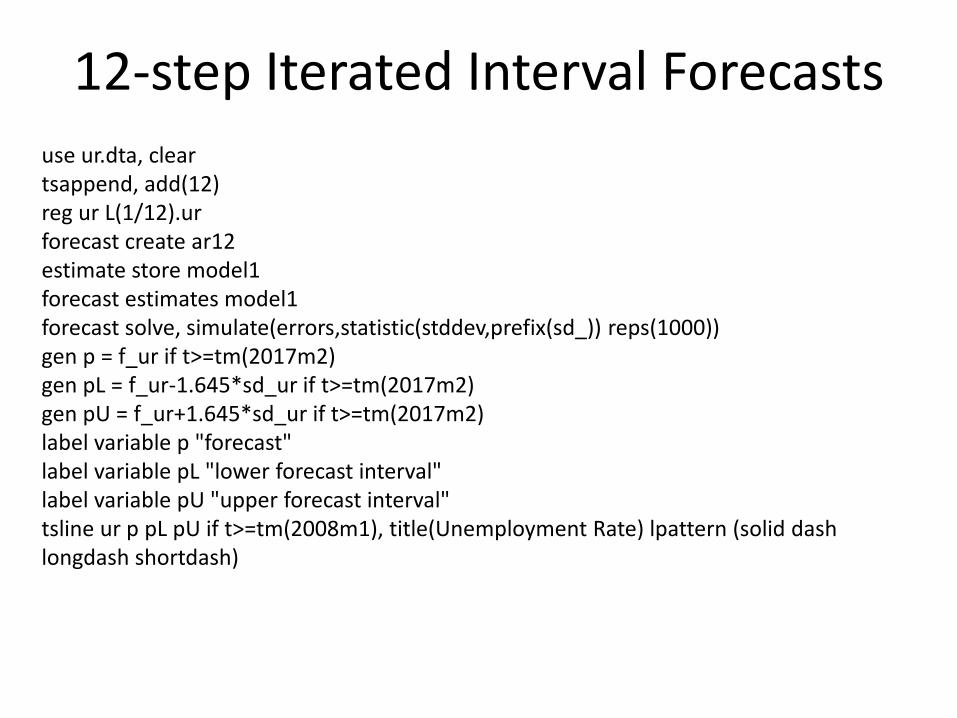
12-step Iterated Interval Forecastsuse ur.dta, cleartsappend, add(12)reg ur L(1/12).urforecast create ar12estimate store model1forecast estimates model1forecast solve, simulate(errors,statistic(stddev,prefix(sd_)) reps(1000))gen p = f_ur if t>=tm(2017m2)gen pL = f_ur-1.645*sd_ur if t>=tm(2017m2)gen pU = f_ur+1.645*sd_ur if t>=tm(2017m2)label variable p "forecast"label variable pL "lower forecast interval"label variable pU "upper forecast interval"tsline ur p pL pU if t>=tm(2008m1), title(Unemployment Rate) lpattern (solid dash longdash shortdash)

Assignments
• Read Diebold Chapter 9• Problem Set # 6
– Due Tuesday (2/28)
• Read Chapter 6 from The Signal and the Noise– Reading Reflection– Due Thursday (3/2)