Multi‐Step Forecast Variance

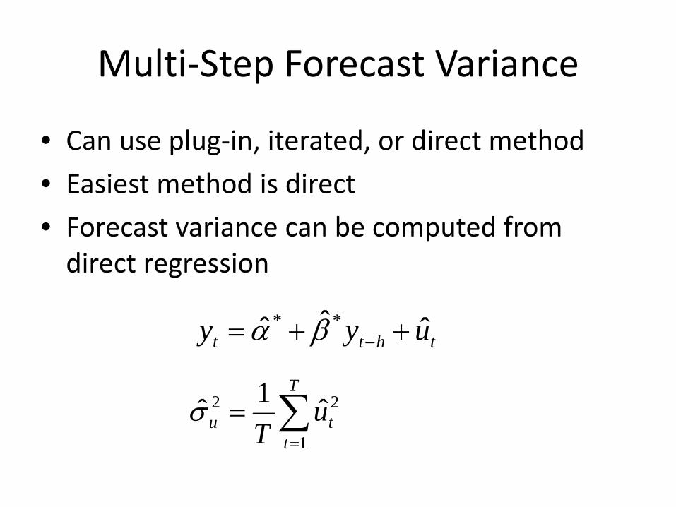
• Can use plug‐in, iterated, or direct method

• Easiest method is direct

• Forecast variance can be computed from direct regression

thtt uyy ˆˆˆ ** ++= −βα

∑=

=T

ttu u

T 1

22 ˆ1σ̂

Forecast Variance and Intervals

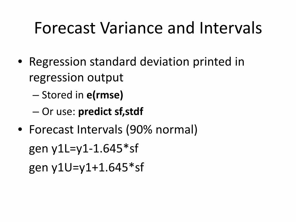
• Regression standard deviation printed in regression output– Stored in e(rmse)

– Or use: predict sf,stdf

• Forecast Intervals (90% normal)

gen y1L=y1‐1.645*sf

gen y1U=y1+1.645*sf

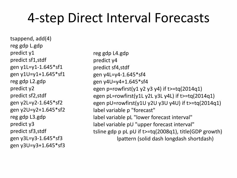
4‐step Direct Interval Forecaststsappend, add(4)reg gdp L.gdppredict y1predict sf1,stdfgen y1L=y1‐1.645*sf1gen y1U=y1+1.645*sf1reg gdp L2.gdppredict y2predict sf2,stdfgen y2L=y2‐1.645*sf2gen y2U=y2+1.645*sf2reg gdp L3.gdppredict y3predict sf3,stdfgen y3L=y3‐1.645*sf3gen y3U=y3+1.645*sf3

reg gdp L4.gdppredict y4predict sf4,stdfgen y4L=y4‐1.645*sf4gen y4U=y4+1.645*sf4egen p=rowfirst(y1 y2 y3 y4) if t>=tq(2014q1)egen pL=rowfirst(y1L y2L y3L y4L) if t>=tq(2014q1)egen pU=rowfirst(y1U y2U y3U y4U) if t>=tq(2014q1)label variable p "forecast"label variable pL "lower forecast interval"label variable pU "upper forecast interval"tsline gdp p pL pU if t>=tq(2008q1), title(GDP growth) 

lpattern (solid dash longdash shortdash)

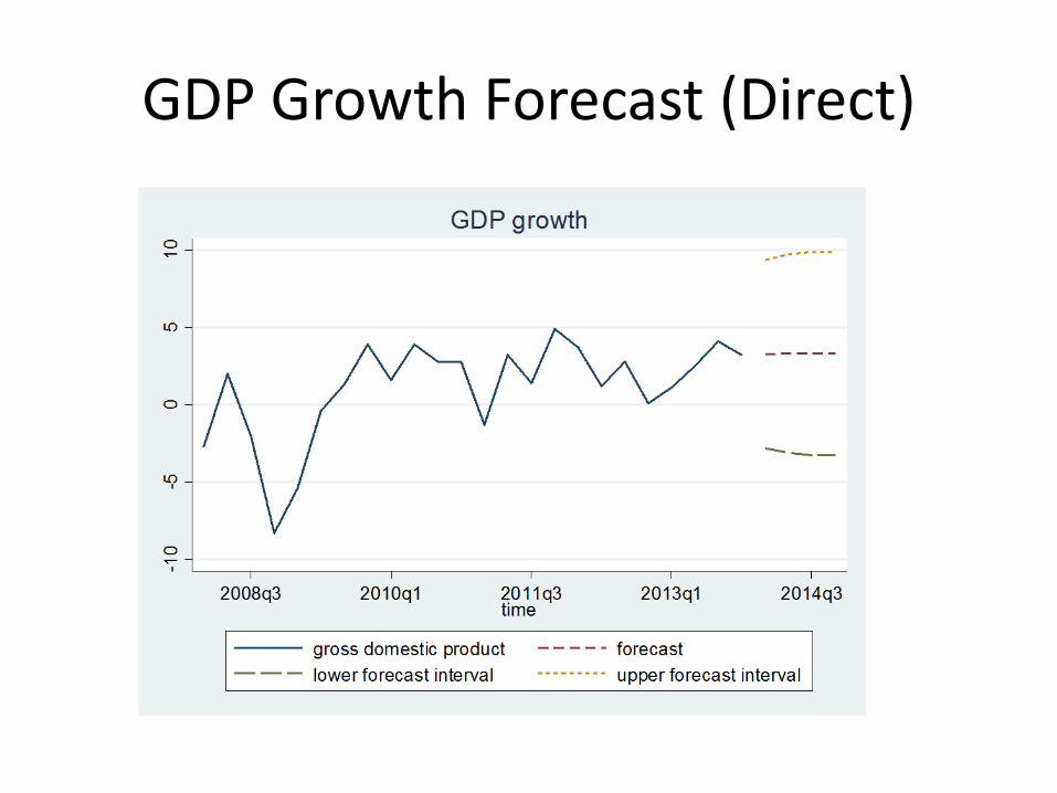
GDP Growth Forecast (Direct)

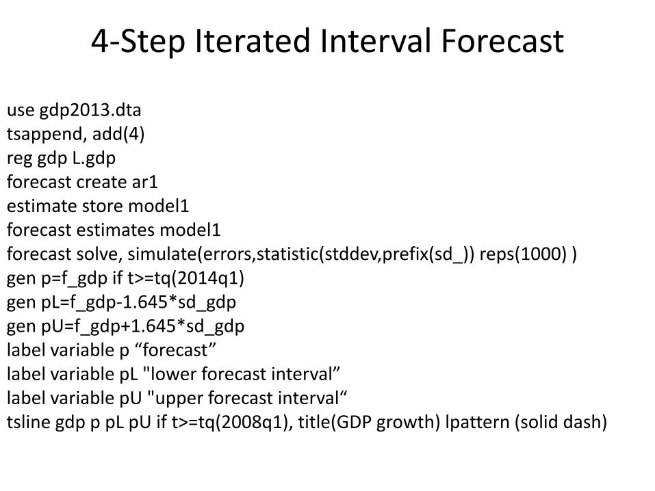
4‐Step Iterated Interval Forecast

use gdp2013.dtatsappend, add(4)reg gdp L.gdpforecast create ar1estimate store model1forecast estimates model1forecast solve, simulate(errors,statistic(stddev,prefix(sd_)) reps(1000) )gen p=f_gdp if t>=tq(2014q1)gen pL=f_gdp‐1.645*sd_gdpgen pU=f_gdp+1.645*sd_gdplabel variable p “forecast”label variable pL "lower forecast interval”label variable pU "upper forecast interval“tsline gdp p pL pU if t>=tq(2008q1), title(GDP growth) lpattern (solid dash)

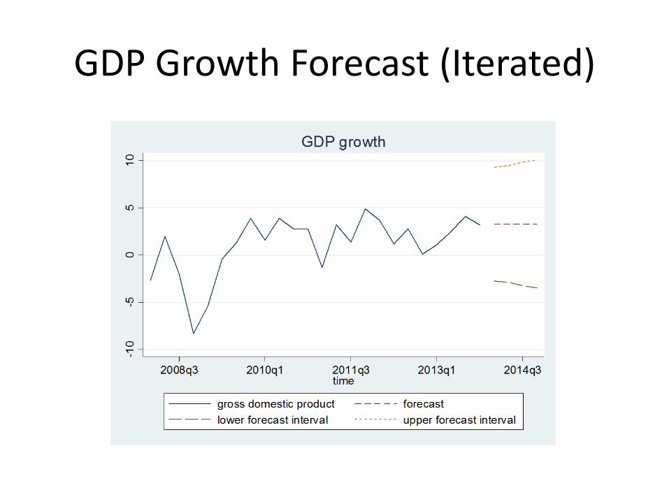
GDP Growth Forecast (Iterated)

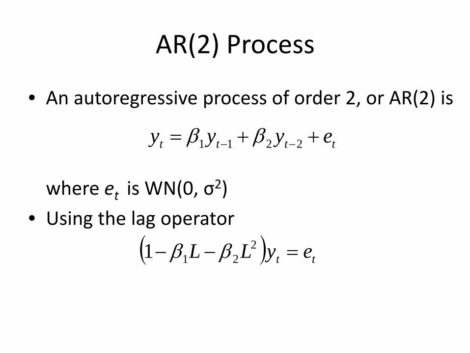
AR(2) Process

• An autoregressive process of order 2, or AR(2) is

where et  is WN(0, σ2) 

• Using the lag operator 

tttt eyyy ++= −− 2211 ββ

( ) tt eyLL =−− 2211 ββ

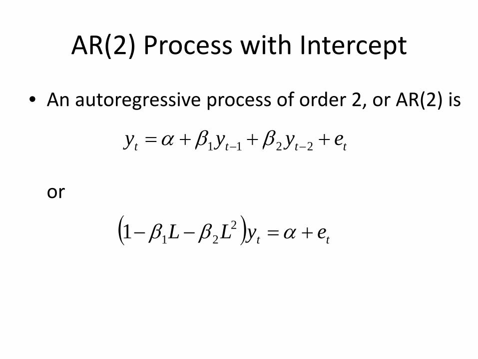
AR(2) Process with Intercept

• An autoregressive process of order 2, or AR(2) is

or

tttt eyyy +++= −− 2211 ββα

( ) tt eyLL +=−− αββ 2211

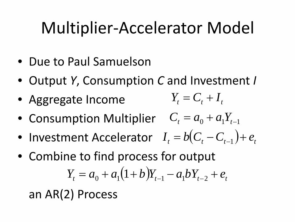
Multiplier‐Accelerator Model

• Due to Paul Samuelson

• Output Y, Consumption C and Investment I

• Aggregate Income

• Consumption Multiplier

• Investment Accelerator

• Combine to find process for output

an AR(2) Process

ttt ICY +=

110 −+= tt YaaC( ) tttt eCCbI +−= −1

( ) tttt ebYaYbaaY +−++= −− 21110 1

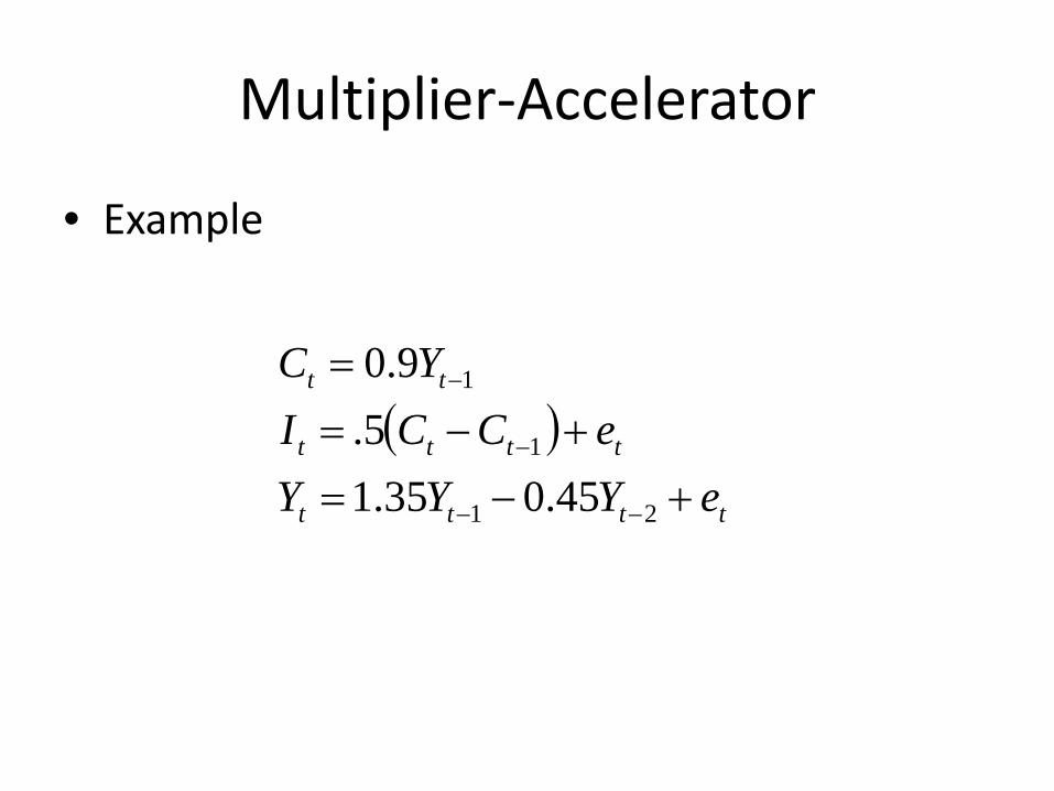
Multiplier‐Accelerator

• Example

( )tttt

tttt

tt

eYYYeCCI

YC

+−=+−=

=

−−

−

−

21

1

1

45.035.15.

9.0

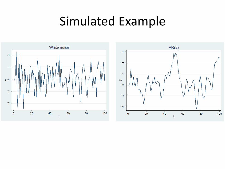
Simulated Example

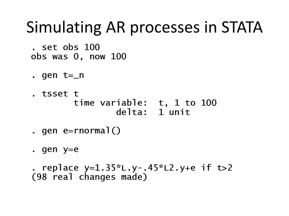
Simulating AR processes in STATA

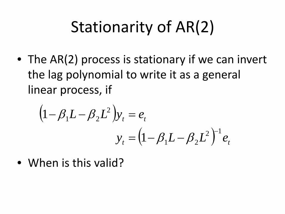
Stationarity of AR(2)

• The AR(2) process is stationary if we can invert the lag polynomial to write it as a general linear process, if

• When is this valid?

( )( ) tt

tt

eLLy

eyLL12

21

221

1

1−

−−=

=−−

ββ

ββ

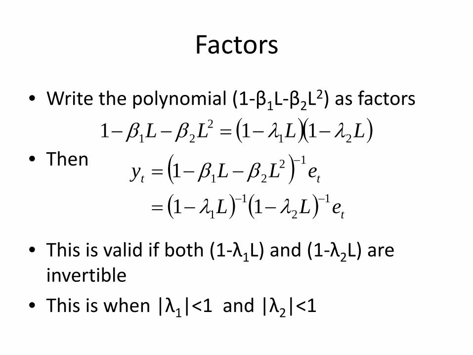
Factors

• Write the polynomial (1‐β1L‐β2L2) as factors

• Then

• This is valid if both (1‐λ1L) and (1‐λ2L) are invertible

• This is when |λ1|<1  and |λ2|<1

( )( )LLLL 212

21 111 λλββ −−=−−

( )( ) ( ) t

tt

eLL

eLLy1

21

1

1221

11

1−−

−

−−=

−−=

λλ

ββ

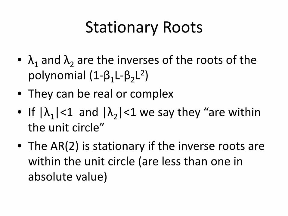
Stationary Roots

• λ1 and λ2 are the inverses of the roots of the polynomial (1‐β1L‐β2L2)

• They can be real or complex

• If |λ1|<1  and |λ2|<1 we say they “are within the unit circle”

• The AR(2) is stationary if the inverse roots are within the unit circle (are less than one in absolute value)

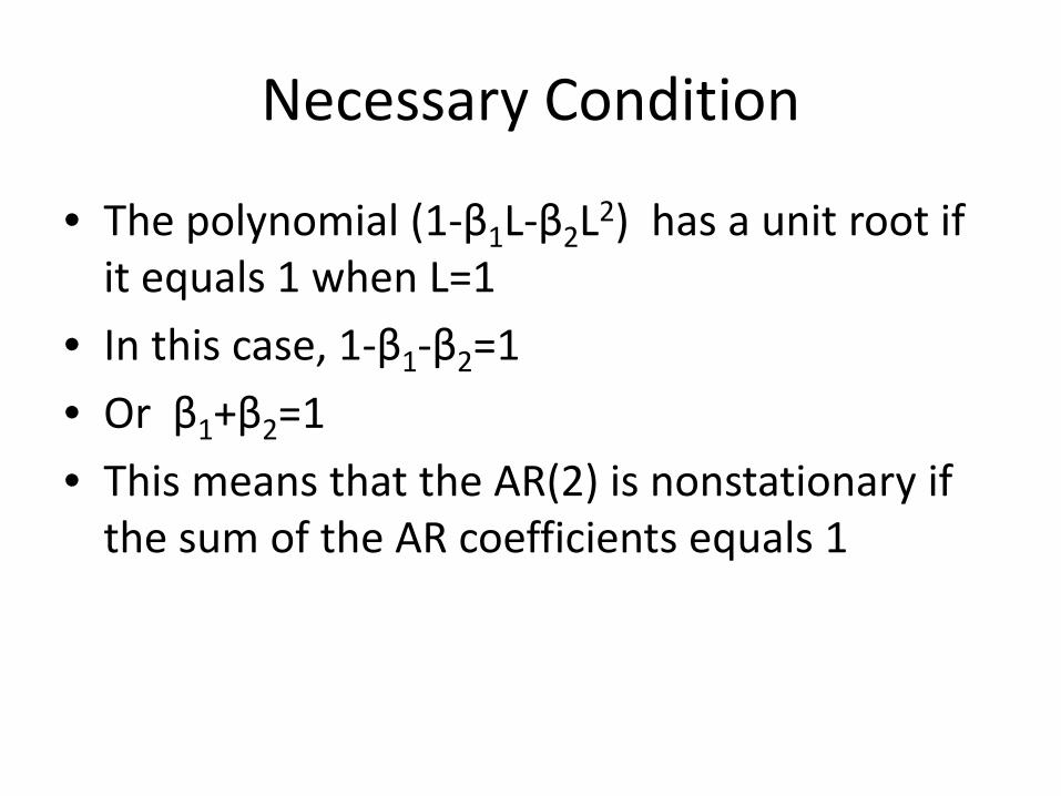
Necessary Condition

• The polynomial (1‐β1L‐β2L2)  has a unit root if it equals 1 when L=1

• In this case, 1‐β1‐β2=1

• Or  β1+β2=1

• This means that the AR(2) is nonstationary if the sum of the AR coefficients equals 1

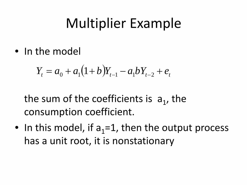
Multiplier Example

• In the model

the sum of the coefficients is  a1, the consumption coefficient.

• In this model, if a1=1, then the output process has a unit root, it is nonstationary

( ) tttt ebYaYbaaY +−++= −− 21110 1

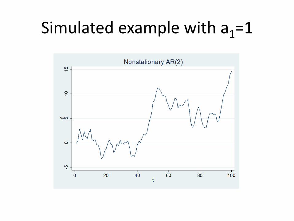
Simulated example with a1=1

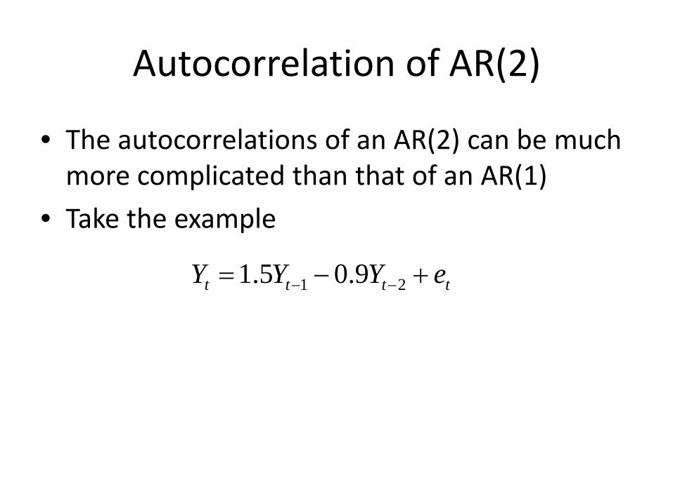
Autocorrelation of AR(2)

• The autocorrelations of an AR(2) can be much more complicated than that of an AR(1)

• Take the example

tttt eYYY +−= −− 21 9.05.1

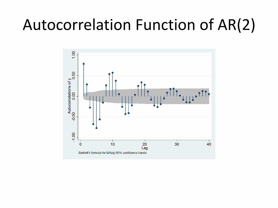
Autocorrelation Function of AR(2)

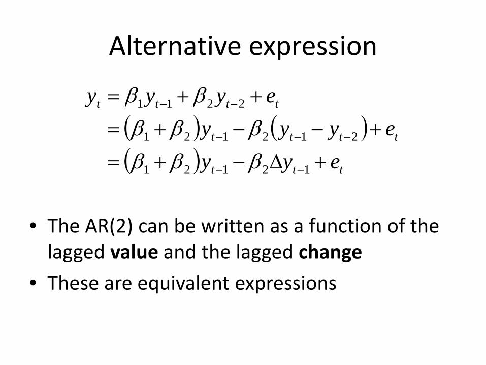
Alternative expression

• The AR(2) can be written as a function of the lagged value and the lagged change 

• These are equivalent expressions

( ) ( )( ) ttt

tttt

tttt

eyyeyyy

eyyy

+Δ−+=+−−+=

++=

−−

−−−

−−

12121

212121

2211

ββββββ

ββ

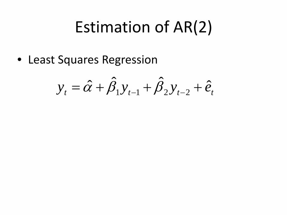
Estimation of AR(2)

• Least Squares Regression

tttt eyyy ˆˆˆˆ 2211 +++= −− ββα

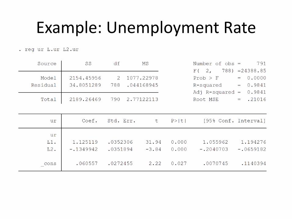
Example: Unemployment Rate

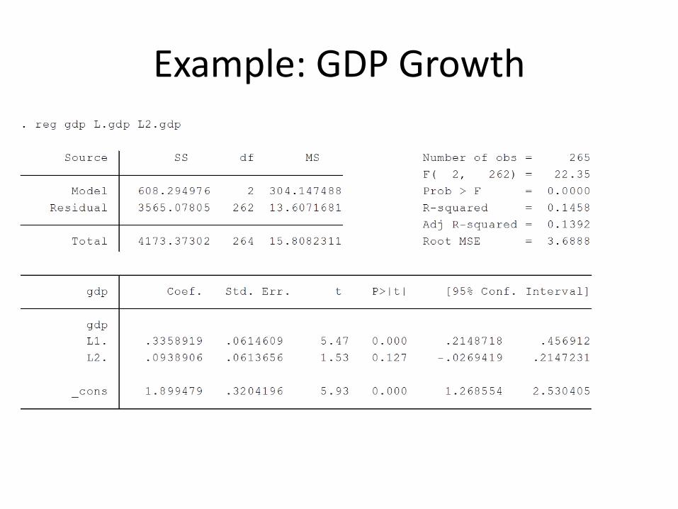
Example: GDP Growth

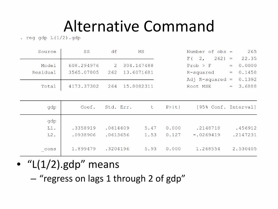
Alternative Command

• “L(1/2).gdp” means – “regress on lags 1 through 2 of gdp”

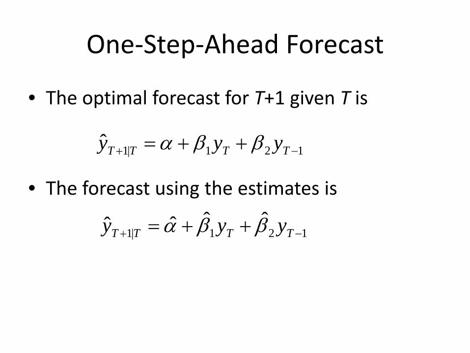
One‐Step‐Ahead Forecast

• The optimal forecast for T+1 given T is

• The forecast using the estimates is

121|1ˆ −+ ++= TTTT yyy ββα

121|1ˆˆˆˆ −+ ++= TTTT yyy ββα

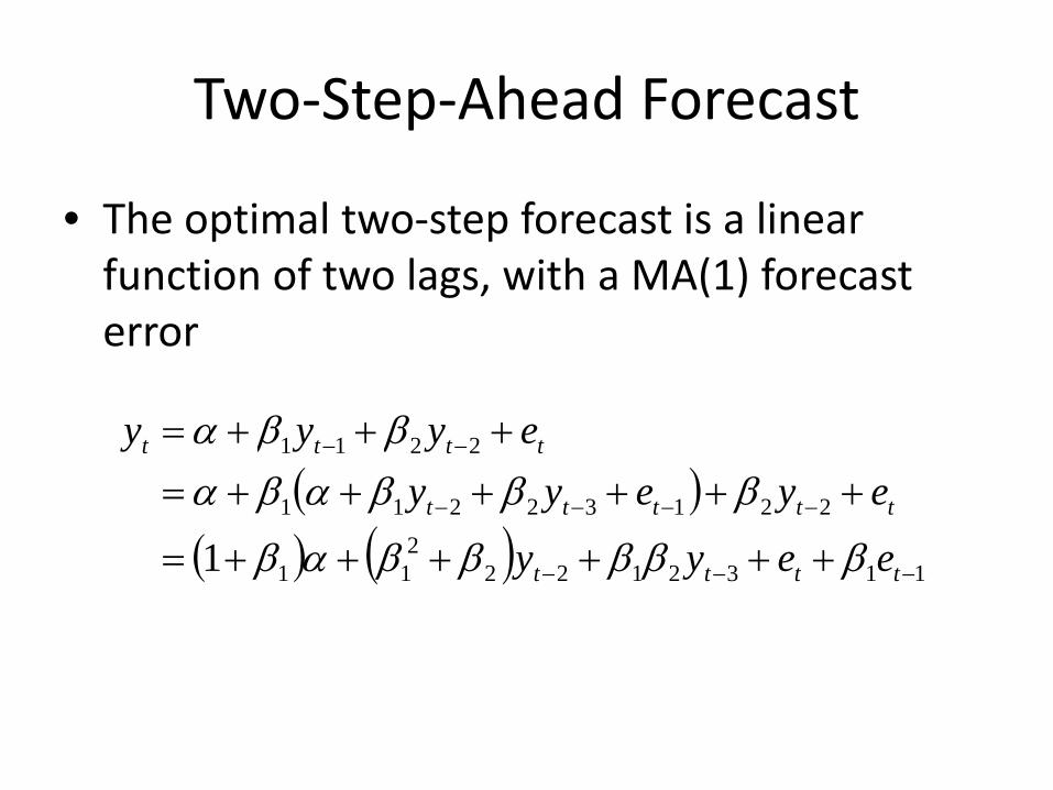
Two‐Step‐Ahead Forecast

• The optimal two‐step forecast is a linear function of two lags, with a MA(1) forecast error

( )( ) ( ) 1132122

211

22132211

2211

1 −−−

−−−−

−−

++++++=

++++++=+++=

tttt

ttttt

tttt

eeyy

eyeyyeyyy

βββββαβ

βββαβαββα

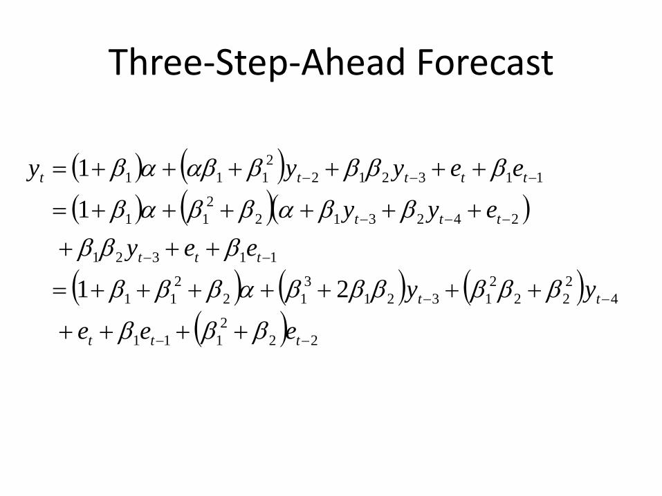
Three‐Step‐Ahead Forecast

( ) ( )( ) ( )( )

( ) ( ) ( )( ) 22

2111

4222

21321

312

211

11321

2423122

11

1132122

111

21

1

1

−−

−−

−−

−−−

−−−

++++

+++++++=

+++++++++=

++++++=

ttt

tt

ttt

ttt

ttttt

eee

yy

eeyeyy

eeyyy

βββ

ββββββαβββ

βββββαββαβ

ββββαβαβ

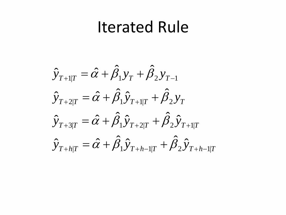
Iterated Rule

ThTThTThT

TTTTTT

TTTTT

TTTT

yyy

yyy

yyy

yyy

|12|11|

|12|21|3

2|11|2

121|1

ˆˆˆˆˆˆ

ˆˆˆˆˆˆ

ˆˆˆˆˆ

ˆˆˆˆ

−+−++

+++

++

−+

++=

++=

++=

++=

ββα

ββα

ββα

ββα

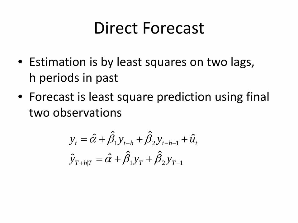
Direct Forecast

• Estimation is by least squares on two lags,       h periods in past

• Forecast is least square prediction using final two observations

121|

121

ˆˆˆˆ

ˆˆˆˆ

−+

−−−

++=

+++=

TTThT

ththtt

yyy

uyyy

ββα

ββα

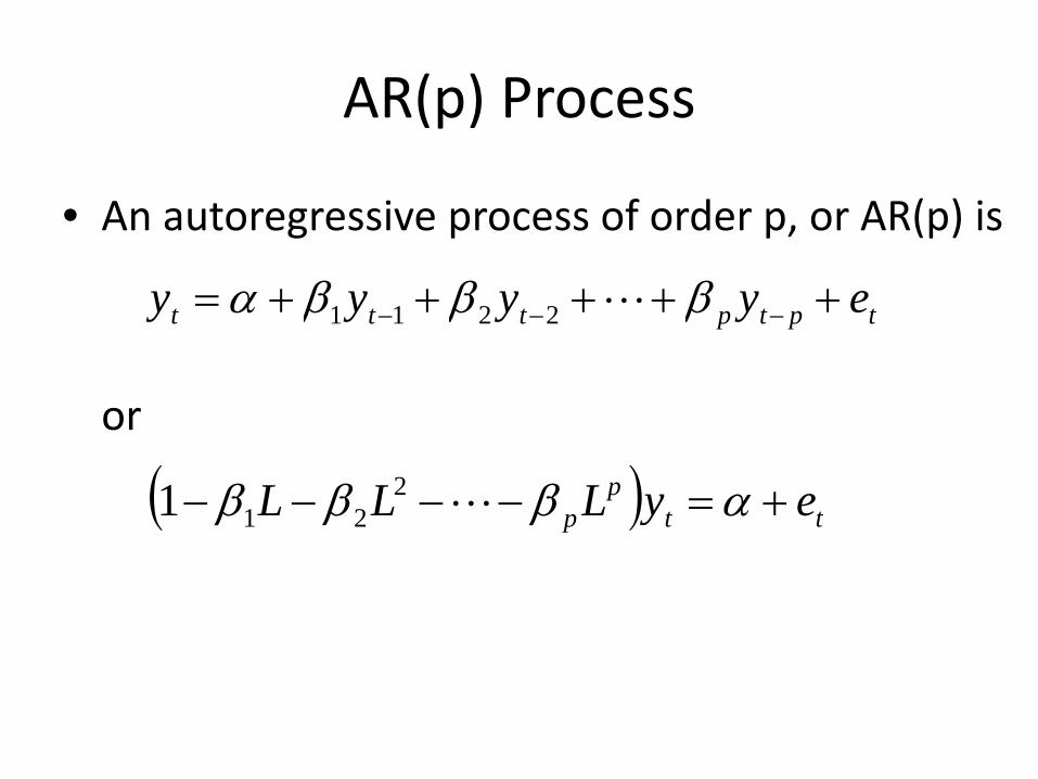
AR(p) Process

• An autoregressive process of order p, or AR(p) is

or

tptpttt eyyyy +++++= −−− βββα L2211

( ) ttp

p eyLLL +=−−−− αβββ L2211

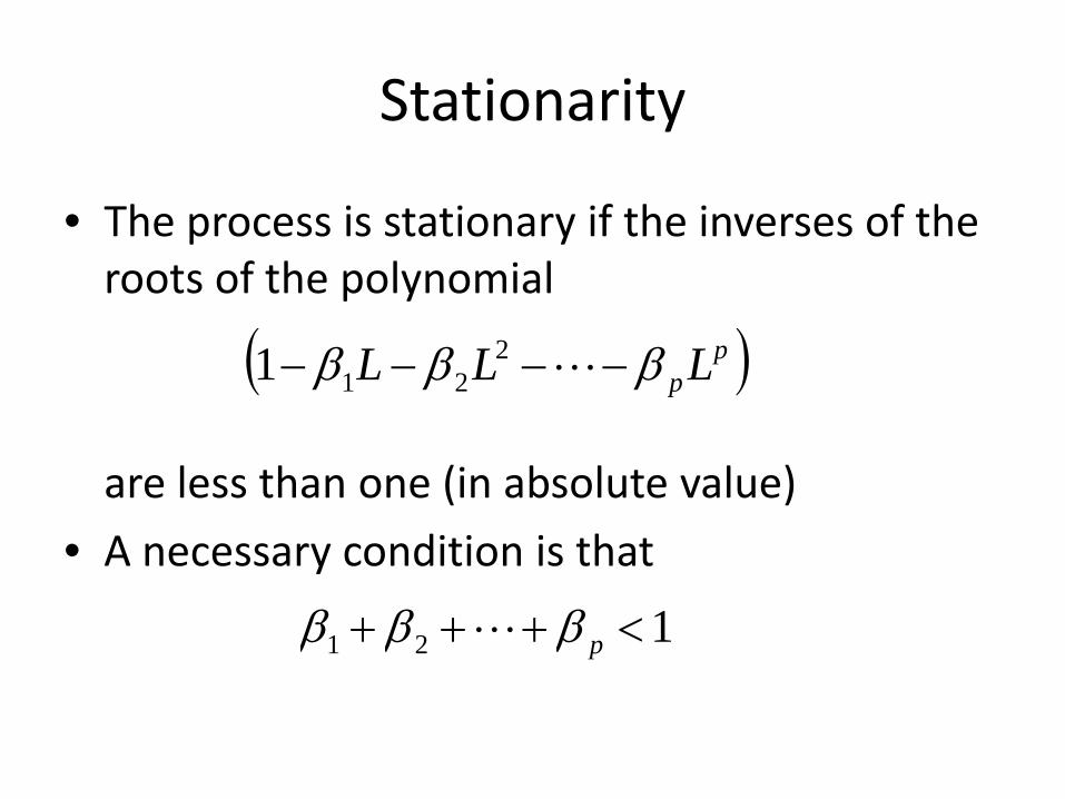
Stationarity

• The process is stationary if the inverses of the roots of the polynomial

are less than one (in absolute value)

• A necessary condition is that 

( )ppLLL βββ −−−− L2

211

121 <+++ pβββ L

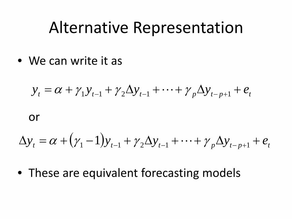
Alternative Representation

• We can write it as

or

• These are equivalent forecasting models

tptpttt eyyyy +Δ++Δ++= +−−− 11211 γγγα L

( ) tptpttt eyyyy +Δ++Δ+−+=Δ +−−− 11211 1 γγγα L

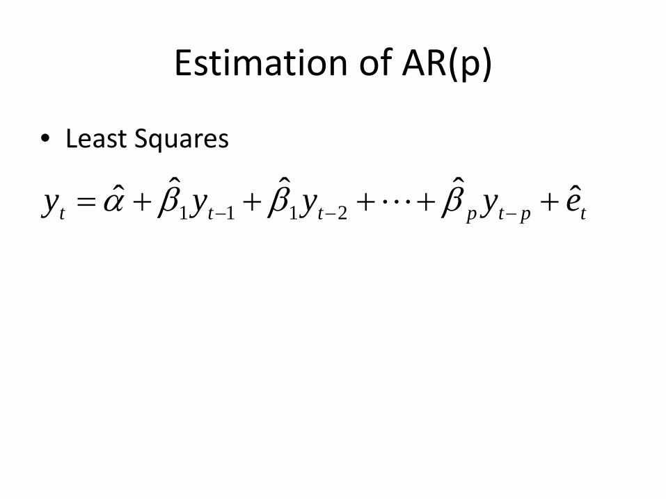
Estimation of AR(p)

• Least Squares

tptpttt eyyyy ˆˆˆˆˆ 2111 +++++= −−− βββα L

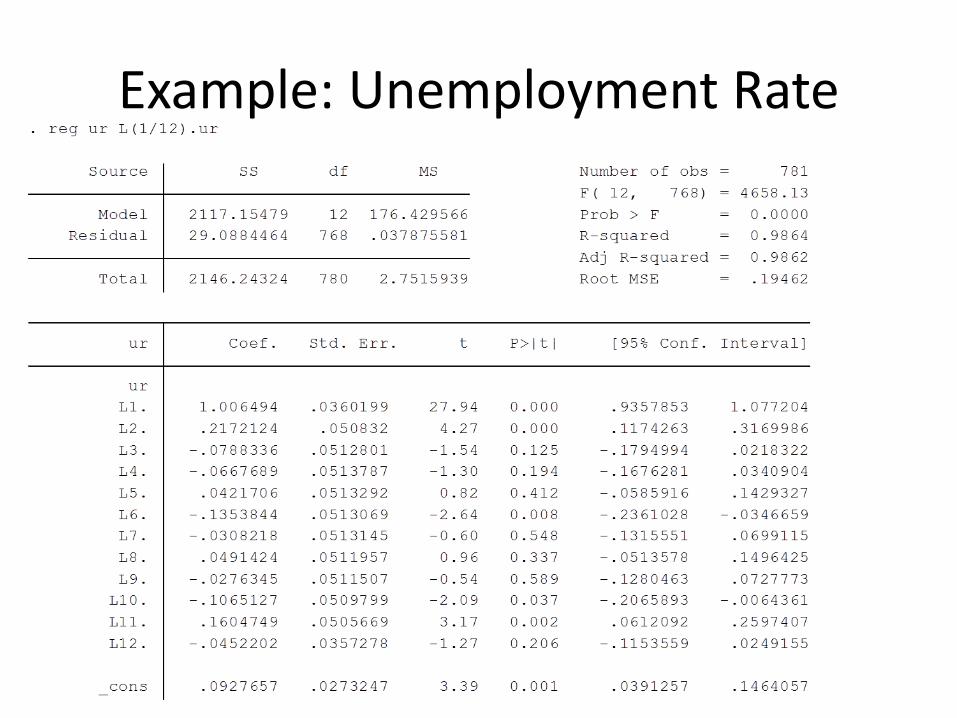
Example: Unemployment Rate

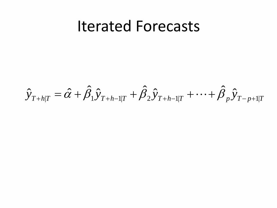
Iterated Forecasts

TpTpThTThTThT yyyy |1|12|11| ˆˆˆˆˆˆˆˆ +−−+−++ ++++= βββα L

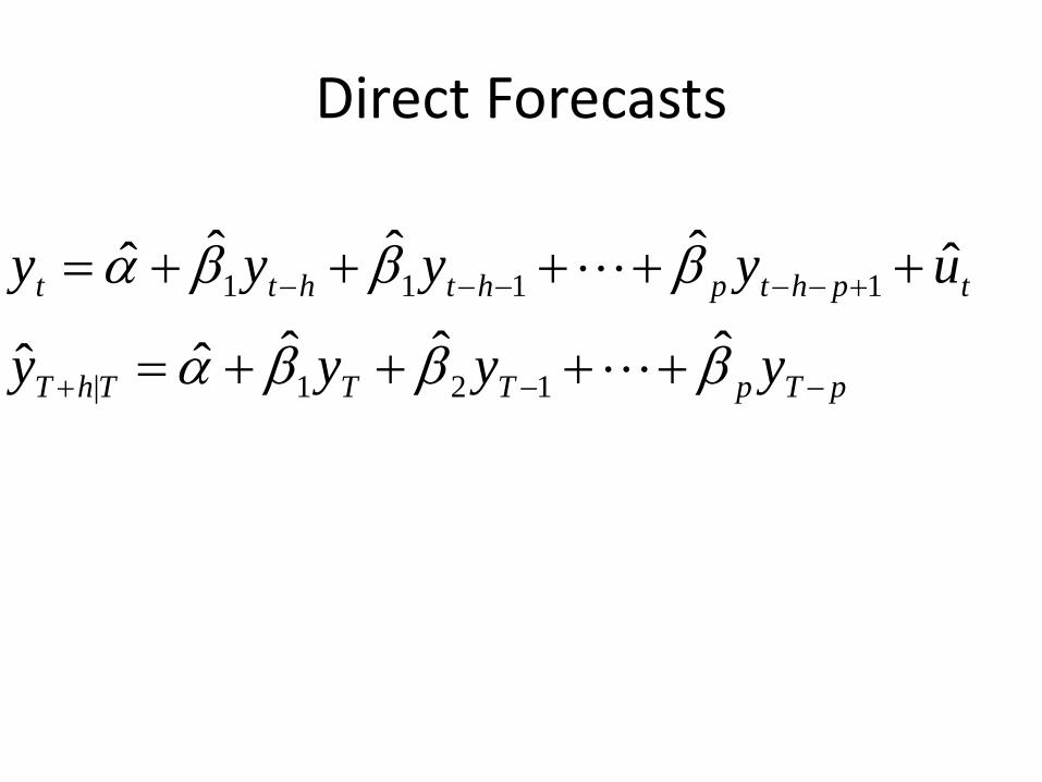
Direct Forecasts

pTpTTThT

tphtphthtt

yyyy

uyyyy

−−+

+−−−−−

++++=

+++++=

βββα

βββαˆˆˆˆˆ

ˆˆˆˆˆ

121|

1111

L

L

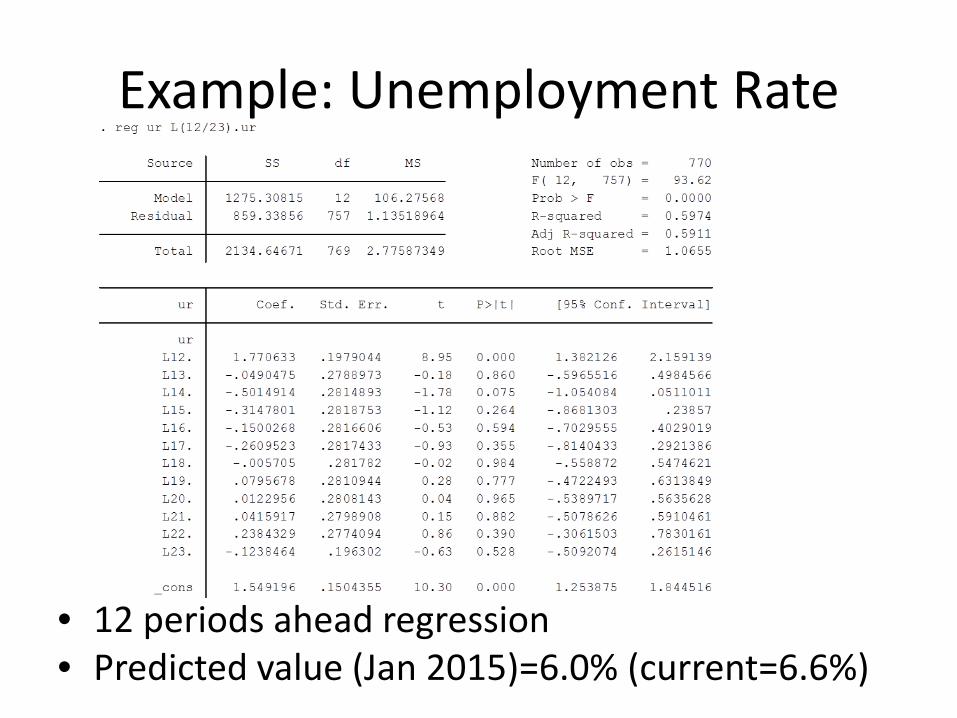
Example: Unemployment Rate

• 12 periods ahead regression• Predicted value (Jan 2015)=6.0% (current=6.6%)

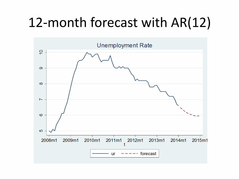
12‐month forecast with AR(12)

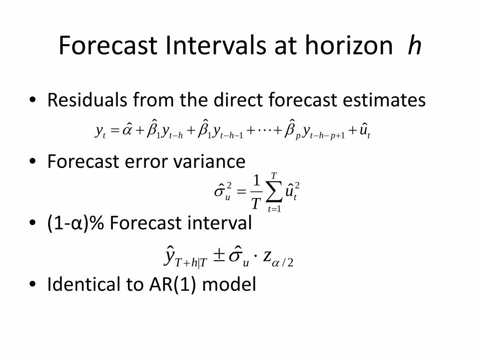
Forecast Intervals at horizon  h

• Residuals from the direct forecast estimates

• Forecast error variance

• (1‐α)% Forecast interval

• Identical to AR(1) model

tphtphthtt uyyyy ˆˆˆˆˆ 1111 +++++= +−−−−− βββα L

∑=

=T

ttu u

T 1

22 ˆ1σ̂

2/| ˆˆ ασ zy uThT ⋅±+

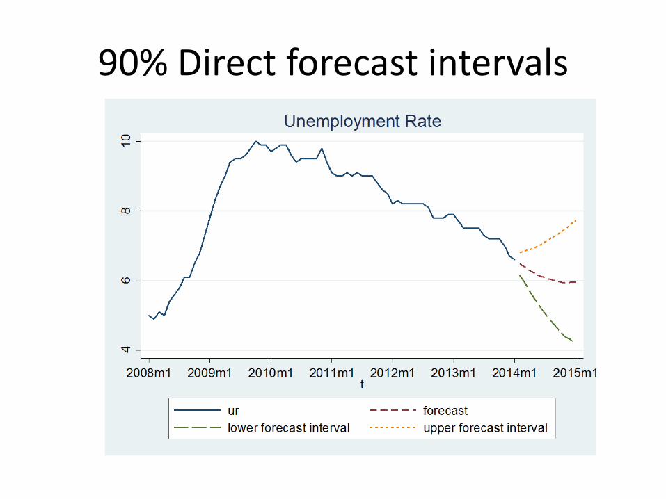
90% Direct forecast intervals

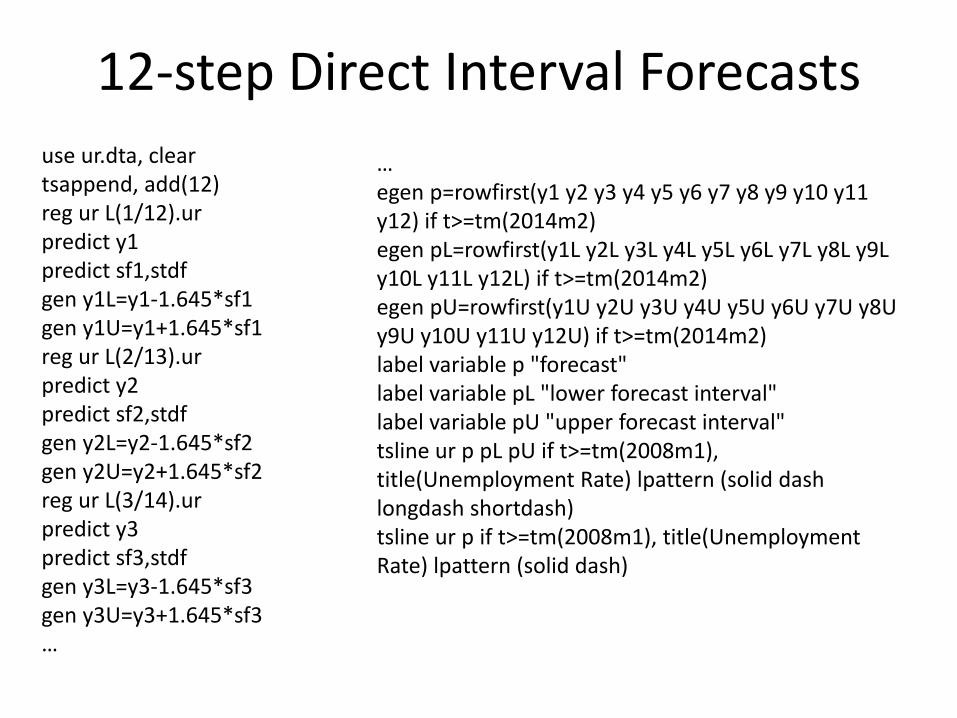
12‐step Direct Interval Forecastsuse ur.dta, cleartsappend, add(12)reg ur L(1/12).urpredict y1predict sf1,stdfgen y1L=y1‐1.645*sf1gen y1U=y1+1.645*sf1reg ur L(2/13).urpredict y2predict sf2,stdfgen y2L=y2‐1.645*sf2gen y2U=y2+1.645*sf2reg ur L(3/14).urpredict y3predict sf3,stdfgen y3L=y3‐1.645*sf3gen y3U=y3+1.645*sf3…

…egen p=rowfirst(y1 y2 y3 y4 y5 y6 y7 y8 y9 y10 y11 y12) if t>=tm(2014m2)egen pL=rowfirst(y1L y2L y3L y4L y5L y6L y7L y8L y9L y10L y11L y12L) if t>=tm(2014m2)egen pU=rowfirst(y1U y2U y3U y4U y5U y6U y7U y8U y9U y10U y11U y12U) if t>=tm(2014m2)label variable p "forecast"label variable pL "lower forecast interval"label variable pU "upper forecast interval"tsline ur p pL pU if t>=tm(2008m1), title(Unemployment Rate) lpattern (solid dash longdash shortdash)tsline ur p if t>=tm(2008m1), title(Unemployment Rate) lpattern (solid dash)

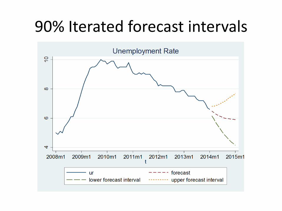
90% Iterated forecast intervals

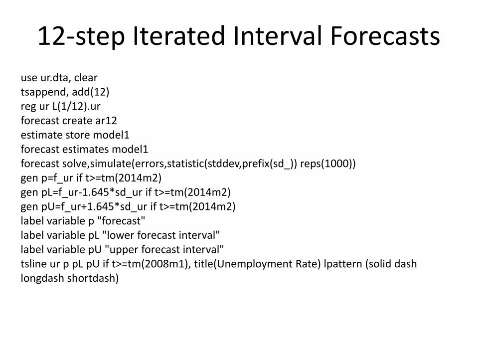
12‐step Iterated Interval Forecastsuse ur.dta, cleartsappend, add(12)reg ur L(1/12).urforecast create ar12estimate store model1forecast estimates model1forecast solve,simulate(errors,statistic(stddev,prefix(sd_)) reps(1000))gen p=f_ur if t>=tm(2014m2)gen pL=f_ur‐1.645*sd_ur if t>=tm(2014m2)gen pU=f_ur+1.645*sd_ur if t>=tm(2014m2)label variable p "forecast"label variable pL "lower forecast interval"label variable pU "upper forecast interval"tsline ur p pL pU if t>=tm(2008m1), title(Unemployment Rate) lpattern (solid dash longdash shortdash)