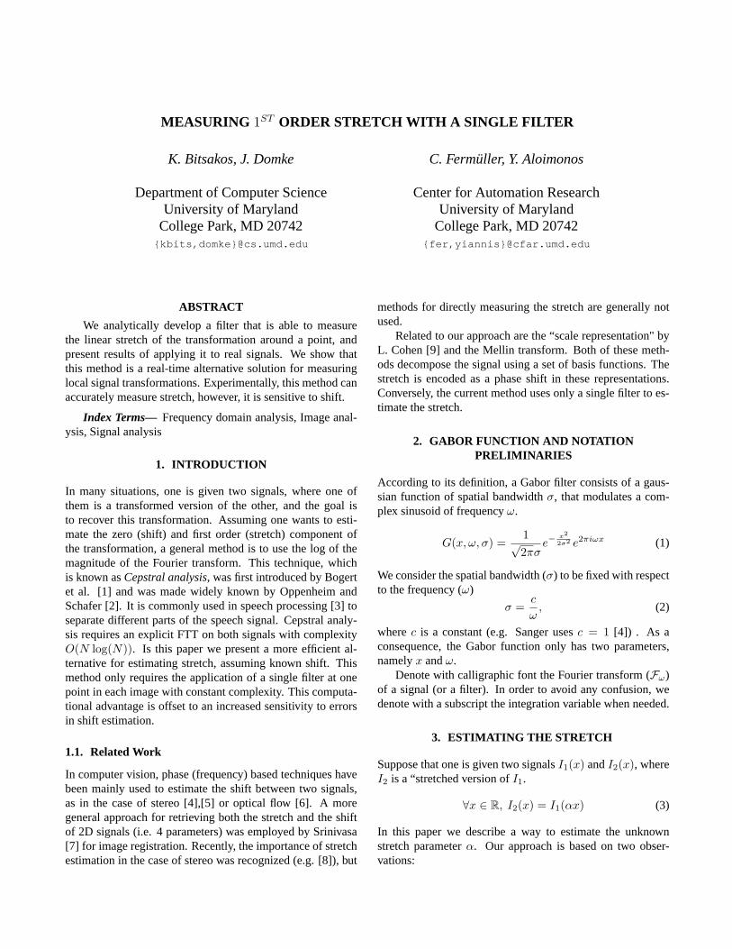
MEASURING 1ST ORDER STRETCH WITH A SINGLE FILTER

K. Bitsakos, J. Domke

Department of Computer ScienceUniversity of Maryland

College Park, MD 20742{kbits,domke}@cs.umd.edu

C. Fermüller, Y. Aloimonos

Center for Automation ResearchUniversity of Maryland

College Park, MD 20742{fer,yiannis}@cfar.umd.edu

ABSTRACT

We analytically develop a filter that is able to measurethe linear stretch of the transformation around a point, andpresent results of applying it to real signals. We show thatthis method is a real-time alternative solution for measuringlocal signal transformations. Experimentally, this method canaccurately measure stretch, however, it is sensitive to shift.

Index Terms— Frequency domain analysis, Image anal-ysis, Signal analysis

1. INTRODUCTION

In many situations, one is given two signals, where one ofthem is a transformed version of the other, and the goal isto recover this transformation. Assuming one wants to esti-mate the zero (shift) and first order (stretch) component ofthe transformation, a general method is to use the log of themagnitude of the Fourier transform. This technique, whichis known asCepstral analysis, was first introduced by Bogertet al. [1] and was made widely known by Oppenheim andSchafer [2]. It is commonly used in speech processing [3] toseparate different parts of the speech signal. Cepstral analy-sis requires an explicit FTT on both signals with complexityO(N log(N)). Is this paper we present a more efficient al-ternative for estimating stretch, assuming known shift. Thismethod only requires the application of a single filter at onepoint in each image with constant complexity. This computa-tional advantage is offset to an increased sensitivity to errorsin shift estimation.

1.1. Related Work

In computer vision, phase (frequency) based techniques havebeen mainly used to estimate the shift between two signals,as in the case of stereo [4],[5] or optical flow [6]. A moregeneral approach for retrieving both the stretch and the shiftof 2D signals (i.e. 4 parameters) was employed by Srinivasa[7] for image registration. Recently, the importance of stretchestimation in the case of stereo was recognized (e.g. [8]), but

methods for directly measuring the stretch are generally notused.

Related to our approach are the “scale representation" byL. Cohen [9] and the Mellin transform. Both of these meth-ods decompose the signal using a set of basis functions. Thestretch is encoded as a phase shift in these representations.Conversely, the current method uses only a single filter to es-timate the stretch.

2. GABOR FUNCTION AND NOTATIONPRELIMINARIES

According to its definition, a Gabor filter consists of a gaus-sian function of spatial bandwidthσ, that modulates a com-plex sinusoid of frequencyω.

G(x, ω, σ) =1√2πσ

e−x2

2σ2 e2πiωx (1)

We consider the spatial bandwidth (σ) to be fixed with respectto the frequency (ω)

σ =c

ω, (2)

wherec is a constant (e.g. Sanger usesc = 1 [4]) . As aconsequence, the Gabor function only has two parameters,namelyx andω.

Denote with calligraphic font the Fourier transform (Fω)of a signal (or a filter). In order to avoid any confusion, wedenote with a subscript the integration variable when needed.

3. ESTIMATING THE STRETCH

Suppose that one is given two signalsI1(x) andI2(x), whereI2 is a “stretched version ofI1.

∀x ∈ R, I2(x) = I1(αx) (3)

In this paper we describe a way to estimate the unknownstretch parameterα. Our approach is based on two obser-vations:

• Convolving the first signal (I1) with a Gabor filter offrequencyω is equivalent to convolving the second sig-nal (I2) with a Gabor filter of frequencyαω (Theorem3.1).

• Considering the log-frequency domain of the Gabor fil-ters the multiplication is transformed into addition (i.e.,stretch is transformed into shift) and thus can be es-timated using the phase shift property of the Fouriertransform (Theorem 3.2).

In the remaining section we formally present our approach inincremental steps using two theorems. We note that the finalresult is asingle filter on the spatial domain, even thought weare using the frequency domain in our proofs.

Theorem 3.1. If the two stretched signals (I1, I2) are as inEq. 3, then

∀ω, [I1(x) ? G(x, ω)](0) = [I2(x) ? G(x, αω)](0) (4)

Proof. According to the definition of a Gabor filter (Eq. 1)and its standard deviation (Eq. 2) we get

G(x, αω) =1√2πσ′

e−x2

2σ′2 e2πiαωx,

σ′ = σαω =c

αω=σω

α

Thus,

G(x, αω) =α√2πσ

e−x2

α2

2σ2 e2πiωαx = αG(αx, ω). (5)

From the definition of convolution we have

[I1(x) ? G(x, ω)](0) =

∫x

I1(x)G(−x, ω)dx. (6)

Similarly,

[I2(x) ? G(x, αω)](0) =

∫x

I2(x)G(−x, αω)dx

=

∫x

I1(αx)G(−x, αω)dx (7)

Settingy = αx, thendy = αdx,

[I2(x) ? G(x, αω)](0) =

∫y

I1(y)G(− y

α, αω)

dy

α.

Using Eq.5 we have

[I2(x) ? G(x, αω)](0) =

∫y

I1(y)G(−y, ω)dy

= [I1(x) ? G(x, ω)](0).

Based on Theorem 3.1 the response of the convolution ofI1, I2 with the gabor filter is a function of the frequencyω,that is

R1(ω) = [I1(x) ? G(x, ω)](0) =

[I2(x) ? G(x, αω)](0) = R2(αω). (8)

If we consider the log frequencyψ instead of the frequencyω

ψ = eω ⇔ ω = logψ, (9)

then Eq. 8 is transformed to

R1(ψ) = R2(ψ + logα). (10)

In principle, we could estimate the shift (in the log-frequencydomainψ) by transforming it into a phase shift using theFourier transform

R1(u) = Fψ{R1} = e2πi logαuR2(u) (11)

and measuring the difference in the phase ofR1 andR2 forany specific frequencyu1. While this is a valid approach, it israther computationally expensive. For every point of the twosignals one has to compute the frequency responseR1, R2 (byconvolving with Gabor filters of different frequencies) andthen take the Fourier transform of those responses. The fol-lowing theorem provides an alternative solution that amountsto convolving the two signals with a single filter.

Theorem 3.2.There exists a filterH(x, u) whose convolutionwith I1, I2 directly encodes the stretch as

[I1(x)?H(x, u)](0) = e2πi logαu[I2(x)?H(x, u)](0). (12)

Specifically, the filter has the analytic form

H(x, u) =

∫ω

G(x, eω)e−2πiωudω. (13)

Proof. From Eqs. 8,9 and 10 we have

R1(eω) = R2(e

ω + logα)

If we consider the Fourier transform ofR1(eω) with respect

to ω, then

R1(u) =

∫ω

e−2πiωuR1(eω)dω

=

∫ω

e−2πiωu[

∫x

I1(x)G(−x, eω)dx]dω

=

∫x

I1(x)[

∫ω

G(−x, eω)e−2πiωudω]dx

=

∫x

I1(x)H(−x, u)dx

= [I1(x) ? H(x, u)](0).

1We have noticed that the following issue is often at first confusing toreaders. We use two different frequency domains. Symbolsω (andψ) denotethe frequency in the “traditional” sense, while symbolu denotes the Fouriertransform ofψ, so in some sense is the“frequency of the frequency domain".

Algorithm 1 Estimating the Stretch

Input :I1, I2 : Input Signalsx0 : A single point along the X-axis

Output :α : The stretch between the two signals

around pointx0

Algorithm :Create the filterH(x, u) =

∫ ω2

ω1

G(x, eω)e−2πiωudω

Convolve the two signals (I1, I2) with H(x, u) aroundx0

Compute the difference in phase of the two measurements (∆θ)Compute the “log-frequency shift”∆ψ = ∆θ

2πu

Compute the stretchα = e∆ψ

Similarly forR2(eω) we get

R2(u) = [I2(x) ? H(x, u)](0).

From the phase shift property of the Fourier transform we get

R1(u) = e2πi logαuR2(u)

and thus

[I1(x) ? H(x, u)](0) = e2πi logαu[I2(x) ? H(x, u)](0).

The algorithm is a straightforward implementation of thetheory and is presented in Alg. 1.

4. EXPERIMENTS

4.1. Stretch without Shift Experiments

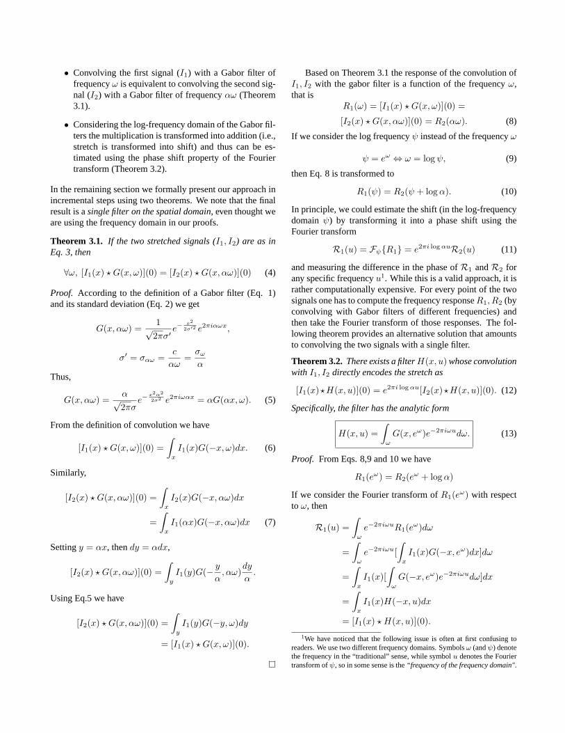
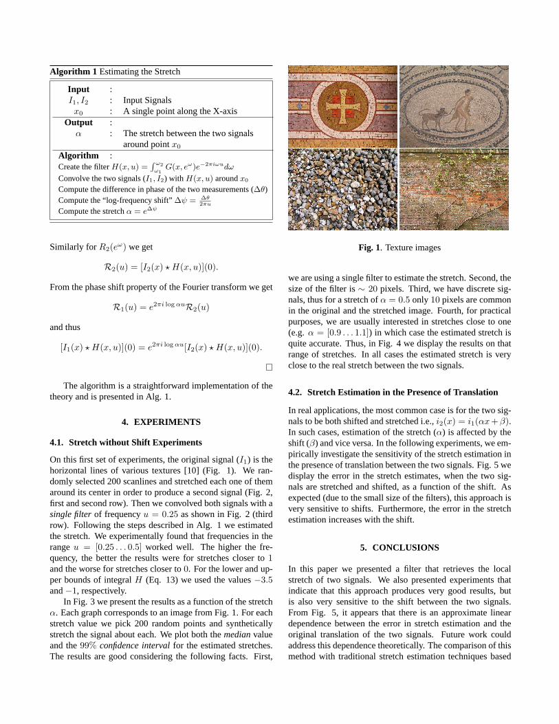
On this first set of experiments, the original signal (I1) is thehorizontal lines of various textures [10] (Fig. 1). We ran-domly selected 200 scanlines and stretched each one of themaround its center in order to produce a second signal (Fig. 2,first and second row). Then we convolved both signals with asingle filterof frequencyu = 0.25 as shown in Fig. 2 (thirdrow). Following the steps described in Alg. 1 we estimatedthe stretch. We experimentally found that frequencies in therangeu = [0.25 . . . 0.5] worked well. The higher the fre-quency, the better the results were for stretches closer to1and the worse for stretches closer to0. For the lower and up-per bounds of integralH (Eq. 13) we used the values−3.5and−1, respectively.

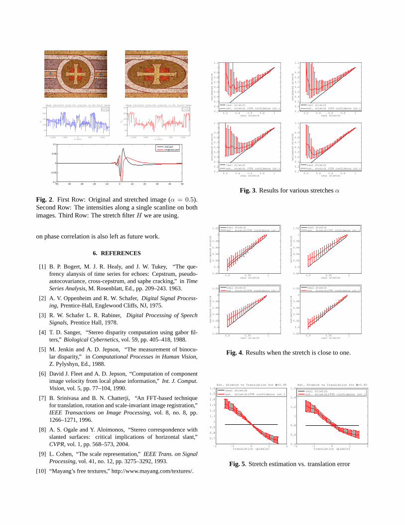
In Fig. 3 we present the results as a function of the stretchα. Each graph corresponds to an image from Fig. 1. For eachstretch value we pick 200 random points and syntheticallystretch the signal about each. We plot both themedianvalueand the99% confidence intervalfor the estimated stretches.The results are good considering the following facts. First,

Fig. 1. Texture images

we are using a single filter to estimate the stretch. Second, thesize of the filter is∼ 20 pixels. Third, we have discrete sig-nals, thus for a stretch ofα = 0.5 only 10 pixels are commonin the original and the stretched image. Fourth, for practicalpurposes, we are usually interested in stretches close to one(e.g.α = [0.9 . . . 1.1]) in which case the estimated stretch isquite accurate. Thus, in Fig. 4 we display the results on thatrange of stretches. In all cases the estimated stretch is veryclose to the real stretch between the two signals.

4.2. Stretch Estimation in the Presence of Translation

In real applications, the most common case is for the two sig-nals to be both shifted and stretched i.e.,i2(x) = i1(αx+β).In such cases, estimation of the stretch (α) is affected by theshift (β) and vice versa. In the following experiments, we em-pirically investigate the sensitivity of the stretch estimation inthe presence of translation between the two signals. Fig. 5 wedisplay the error in the stretch estimates, when the two sig-nals are stretched and shifted, as a function of the shift. Asexpected (due to the small size of the filters), this approachisvery sensitive to shifts. Furthermore, the error in the stretchestimation increases with the shift.

5. CONCLUSIONS

In this paper we presented a filter that retrieves the localstretch of two signals. We also presented experiments thatindicate that this approach produces very good results, butis also very sensitive to the shift between the two signals.From Fig. 5, it appears that there is an approximate lineardependence between the error in stretch estimation and theoriginal translation of the two signals. Future work couldaddress this dependence theoretically. The comparison of thismethod with traditional stretch estimation techniques based

−1000 −500 0 500 10000

50

100

150

200

250

x−axis

s1

Image intensity along the scanline on the first image

s1

−1000 −500 0 500 10000

50

100

150

200

250

x−axis

s2

Image intensity along the scanline on the second image

s2

−50 −40 −30 −20 −10 0 10 20 30 40 50−0.1

−0.05

0

0.05

0.1real partimaginary part

Fig. 2. First Row: Original and stretched image (α = 0.5).Second Row: The intensities along a single scanline on bothimages. Third Row: The stretch filterH we are using.

on phase correlation is also left as future work.

6. REFERENCES

[1] B. P. Bogert, M. J. R. Healy, and J. W. Tukey, “The que-frency alanysis of time series for echoes: Cepstrum, pseudo-autocovariance, cross-cepstrum, and saphe cracking,” inTimeSeries Analysis, M. Rosenblatt, Ed., pp. 209–243. 1963.

[2] A. V. Oppenheim and R. W. Schafer,Digital Signal Process-ing, Prentice-Hall, Englewood Cliffs, NJ, 1975.

[3] R. W. Schafer L. R. Rabiner,Digital Processing of SpeechSignals, Prentice Hall, 1978.

[4] T. D. Sanger, “Stereo disparity computation using gabor fil-ters,” Biological Cybernetics, vol. 59, pp. 405–418, 1988.

[5] M. Jenkin and A. D. Jepson, “The measurement of binocu-lar disparity,” inComputational Processes in Human Vision,Z. Pylyshyn, Ed., 1988.

[6] David J. Fleet and A. D. Jepson, “Computation of componentimage velocity from local phase information,”Int. J. Comput.Vision, vol. 5, pp. 77–104, 1990.

[7] B. Srinivasa and B. N. Chatterji, “An FFT-based techniquefor translation, rotation and scale-invariant image registration,”IEEE Transactions on Image Processing, vol. 8, no. 8, pp.1266–1271, 1996.

[8] A. S. Ogale and Y. Aloimonos, “Stereo correspondence withslanted surfaces: critical implications of horizontal slant,”CVPR, vol. 1, pp. 568–573, 2004.

[9] L. Cohen, “The scale representation,”IEEE Trans. on SignalProcessing, vol. 41, no. 12, pp. 3275–3292, 1993.

[10] “Mayang’s free textures,” http://www.mayang.com/textures/.

0.2 0.4 0.6 0.8 10.1

0.2

0.3

0.4

0.5

0.6

0.7

0.8

0.9

1

1.1

real stretch

est

ima

ted

str

etc

h

real stretchest. stretch (99% confidence int.)

0.2 0.4 0.6 0.8 10.1

0.2

0.3

0.4

0.5

0.6

0.7

0.8

0.9

1

1.1

real stretch

est

ima

ted

str

etc

h

real stretchest. stretch (99% confidence int.)

0.2 0.4 0.6 0.8 10.1

0.2

0.3

0.4

0.5

0.6

0.7

0.8

0.9

1

1.1

real stretch

est

ima

ted

str

etc

h

real stretchest. stretch (99% confidence int.)

0.2 0.4 0.6 0.8 10.1

0.2

0.3

0.4

0.5

0.6

0.7

0.8

0.9

1

1.1

real stretch

est

ima

ted

str

etc

h

real stretchest. stretch (99% confidence int.)

Fig. 3. Results for various stretchesα

0.9 0.95 10.88

0.9

0.92

0.94

0.96

0.98

1

1.02

real stretch

est

ima

ted

str

etc

h

real stretchest. stretch(99% confidence int.)

0.9 0.95 10.88

0.9

0.92

0.94

0.96

0.98

1

1.02

real stretch

est

ima

ted

str

etc

h

real stretchest. stretch(99% confidence int.)

0.9 0.95 10.88

0.9

0.92

0.94

0.96

0.98

1

1.02

real stretch

est

ima

ted

str

etc

h

real stretchest. stretch(99% confidence int.)

0.9 0.95 10.88

0.9

0.92

0.94

0.96

0.98

1

1.02

real stretch

est

ima

ted

str

etc

h

real stretchest. stretch(99% confidence int.)

Fig. 4. Results when the stretch is close to one.

−2 −1 0 1 2

0.7

0.8

0.9

1

1.1

1.2

1.3

1.4

1.5

1.6

translation (pixels)

est

ima

ted

str

etc

h

Est. Stretch vs Translation for α=0.95

real stretchest. stretch(99% confidence int.)

−2 −1 0 1 20.4

0.6

0.8

1

1.2

1.4

1.6

translation (pixels)

est

ima

ted

str

etc

h

Est. Stretch vs Translation for α=0.80

real stretchest. stretch(99% confidence int.)

Fig. 5. Stretch estimation vs. translation error