The geometrically nonlinear Cosserat micropolar

shear-stretch energy. Part I: A general parameter reduction

formula and energy-minimizing microrotations in 2D

Andreas Fischle∗ and Patrizio Neff†

November 16, 2018

Abstract

In any geometrically nonlinear quadratic Cosserat-micropolar extended continuum model for-mulated in the deformation gradient field F := ∇ϕ : Ω→ GL+(n) and the microrotation fieldR : Ω→ SO(n), the shear-stretch energy is necessarily of the form

Wµ,µc(R ;F ) := µ

∥∥sym(RTF − 1)∥∥2

+ µc∥∥skew(RTF − 1)

∥∥2,

where µ > 0 is the Lame shear modulus and µc ≥ 0 is the Cosserat couple modulus. In thepresent contribution, we work towards explicit characterizations of the set of optimal Cosseratmicrorotations argminR∈ SO(n) Wµ,µc

(R ;F ) as a function of F ∈ GL+(n) and weights µ > 0and µc ≥ 0. For n ≥ 2, we prove a parameter reduction lemma which reduces the optimalityproblem to two limit cases: (µ, µc) = (1, 1) and (µ, µc) = (1, 0). In contrast to Grioli’stheorem, we derive non-classical minimizers for the parameter range µ > µc ≥ 0 in dimensionn=2. Currently, optimality results for n ≥ 3 are out of reach for us, but we contribute explicitrepresentations for n= 2 which we name rpolar±µ,µc(F ) ∈ SO(2) and which arise for n= 3 byfixing the rotation axis a priori. Further, we compute the associated reduced energy levelsand study the non-classical optimal Cosserat rotations rpolar±µ,µc(Fγ) for simple planar shear.

Key words: Cosserat, Grioli’s theorem, micropolar, polar media, non-symmetric stretch, zeroCosserat couple modulus, polar decomposition, euclidean distance to SO(n)

AMS 2000 subject classification: 15A24, 22L30, 74A30, 74A35, 74B20, 74G05, 74G65, 74N15.

Contents

1 Introduction 2

2 Parameter reduction for µ and µc 3

3 Optimal rotations for the Cosserat shear-stretch energy 7

4 Optimal rotations for planar simple shear 13

5 Conclusion 15

References 16

A Appendix 17

∗Corresponding author: Andreas Fischle, Fakultat fur Mathematik, Informatik, Naturwissenschaften, IGPM,RWTH Aachen, Templergraben 55, 52062 Aachen, Germany, email: fischle@igpm.rwth-aachen.de†Patrizio Neff, Head of Lehrstuhl fur Nichtlineare Analysis und Modellierung, Fakultat fur Mathematik, Univer-

sitat Duisburg-Essen, Thea-Leymann Str. 9, 45127 Essen, Germany, email: patrizio.neff@uni-due.de

1

arX

iv:1

507.

0548

0v1

[m

ath.

AP]

20

Jul 2

015

1 Introduction

In 1940 Guiseppe Grioli proved a remarkable optimality result [6] for the polar factor in dimensionn = 3. To state his result, we denote by Rp(F ) ∈ SO(n) the unique orthogonal factor of F ∈GL+(n) in the right polar decomposition F = Rp(F )U(F ) and by U(F ) = Rp(F )TF =

√FTF ∈

PSym(n) the symmetric positive definite Biot stretch tensor. In [6] Grioli proved the special casen = 3 of the following theorem:

Theorem 1.1 (Grioli’s theorem [6, 12, 3]). Let n ≥ 2 and ‖X‖2 := tr[XTX

]the Frobenius norm.

Then for any F ∈ GL+(n), it holds

argminR∈ SO(n)

∥∥RTF − 1∥∥2= Rp(F ), and thus min

R∈ SO(n)

∥∥RTF − 1∥∥2= ‖U − 1‖2 . (1.1)

The optimality of the polar factor Rp(F ) for n = 3 generalizes to any dimension n ≥ 2, see,e.g., [12], and it is this more general theorem to which we shall refer as Grioli’s theorem in thispresent work. A modern exposition of the original contribution of Grioli has been recently madeavailable in [21].

In contrast to Grioli’s theorem, it has been noted in [18] that the polar factor Rp(F ) is notnecessarily optimal for a more general formulation of Grioli’s theorem with weights. Hence, ourmain objective is to make progress on

Problem 1.2 (Weighted optimality). Let n ≥ 2. Compute the set of optimal rotations

argminR∈ SO(n)

Wµ,µc(R ;F ) := argminR∈ SO(n)

µ∥∥sym(RTF − 1)

∥∥2+ µc

∥∥skew(RTF − 1)∥∥2

(1.2)

for given F ∈ GL+(n) and weights µ > 0, µc ≥ 0 such that µ 6= µc. Here, sym(X) := 12 (X +XT )

and skew(X) := 12 (X −XT ).

For µ = µc, we recover Grioli’s theorem. This case is well understood. However, no systematicanalysis of the proposed weighted optimality problem seems to exist in the literature.

Note that Problem 1.2 is of independent interest in the mechanics of micropolar media and Cosserattheory in particular. The weighted strain energy contribution Wµ,µc arises in any geometricallynonlinear Cosserat-micropolar model proposed in, e.g., [15], cf. [2, 4, 10, 26, 13, 15, 25] and forany 6-parameter geometrically nonlinear Cosserat shell model proposed in [1, 27, 28, 29]. In thebeforementioned material models Wµ,µc

determines the shear-stretch energy contribution. Toobtain a full Cosserat continuum model, Wµ,µc

needs to be augmented by a curvature energyterm [22] and a volumetric energy term, see, e.g., [16] or [18]. However, Problem 1.2 reappears as alimit case for vanishing characteristic length Lc = 0.1 In this scenario, the curvature term vanishesidentically and the set of global minimizers for (1.2) admits an interpretation as optimal Cosseratrotations for given deformation gradient F ∈ GL+(n) and material parameters µ and µc. Grioli’stheorem implies that for µ = µc the optimal Cosserat rotation is uniquely given by Rp(F ), i.e.,it is the orthogonal part of the right polar decomposition F = Rp U . The corresponding reducedenergy level is the Biot-energy, see [18].

The suitable choice of the so-called Cosserat couple modulus µc ≥ 0 for specific materials orboundary value problems is an interesting open question [14]. In particular, a strictly positivechoice µc > 0 is debatable [14] and a better understanding of the limit case µc = 0 is hence ofinterest. This further motivates to study the weighted formulation stated in Problem 1.2.

We want to stress that although the term Wµ,µc subject to minimization in (1.2) is quadratic inthe nonsymmetric microstrain tensor U−1 = RTF −1 (see, e.g., [4]), the associated minimizationproblem with respect to R is nonlinear due to the multiplicative coupling of R and F and thegeometry of SO(n).

1For this interpretation to work, we have to assume that the volume term decouples from the microrotation R,

e.g., W vol(U) := λ4

[(det[U ]− 1

)2+

(1

det[U ]− 1

)2], which seems natural, since it is trivially satisfied in the linear

Cosserat models [20, 14, 19]. The linear elastic energy density is of the form W lin(∇u,A) := µ ‖sym(∇u−A)‖2 +µc ‖skew(∇u−A)‖2 + λ

2tr [(∇u−A)]2. Here, for all admissible values of µ > 0 and µc > 0, the unique minimizer

is given by A = skew(∇u).

2

Remark 1.3 (Existence of global minimizers). The energy Wµ,µc(R ;F ) is a polynomial in thematrix entries, hence Wµ,µc

∈ C∞(SO(n),R). Further, since the Lie group SO(n) is compact and∂SO(n) = ∅, the global extrema of Wµ,µc

are attained at interior points.

The previous remark hints at a possible solution strategy for Problem 1.2. Suppose that wesucceed to compute all the critical points Rcrit ∈ SO(n) of Wµ,µc(R ;F ).2 Then, if possible, adirect comparison of the associated critical energy levels Wµ,µc

(Rcrit ;F ) might allow us to identifythe energy-minimizing branches for given parameters F, µ and µc. Note that any minimal branchcoincides with the reduced Cosserat shear-stretch energy

W redµ,µc : GL+(n)→ R+

0 , W redµ,µc(F ) := min

R∈ SO(n)Wµ,µc(R ;F ) . (1.3)

At present a solution for the three-dimensional problem (let alone the n-dimensional problem)seems out of reach for us. Therefore, we restrict our attention to the planar case where we canbase our computations on the standard parametrisation

R : [−π, π]→ SO(2) ⊂ R2×2, R(α) :=

(cosα − sinαsinα cosα

)(1.4)

by a rotation angle.3

Regarding the material parameters, we prove that, for any dimension n ≥ 2, it is sufficient to restrictour attention to two parameter pairs: (µ, µc) = (1, 1), the classical case, and (µ, µc) = (1, 0), thenon-classical case. We shall see that, somewhat surprisingly, the solutions for arbitrary µ > 0 andµc ≥ 0 can be recovered from these two limiting cases. A large part of this paper is dedicated tothe discussion of the non-classical choice of material parameters in the planar case.

Problem 1.4 (The planar minimization problem). Let F ∈ GL+(2), µ > 0 and µc ≥ 0. The taskis to compute the set of optimal microrotation angles

argminα ∈ [−π,π]

∥∥∥∥∥(√µ sym +

õc skew).

[(cosα − sinαsinα cosα

)T (F11 F12

F21 F22

)−(

1 00 1

)]∥∥∥∥∥2

. (1.5)

It turns out that there are at most two optimal planar rotations in what we will discern as thenon-classical parameter range µ > µc ≥ 0. Both of them coincide with the polar factor Rp(F )in the compressive regime of F ∈ GL+(2), but deviate elsewhere; see Section 3. We denote theexplicit formulae for the optimal Cosserat rotations (i.e., solutions to (1.2)) by rpolarµ,µc(F ) andthe respective rotation angles (i.e., solutions to (1.5)) by αµ,µc(F ) (possibly multi-valued). Thecomputation of global minimizers in dependence of F is not completely obvious even for the reducedplanar case. We hope that the discovered mechanisms will help to understand the cases n ≥ 3eventually.

This paper is now structured as follows: we first prove a dimension-independent parameter trans-formation lemma for µ and µc in Section 2 which allows us to focus on a classical (µ, µc) = (1, 1) anda non-classical limit case (µ, µc) = (1, 0). In Section 3, we compute the optimal planar Cosseratrotations and associated formally reduced energies, first for the classical and non-classical limitcases for µ and µc, then for all admissible values of the material parameters. Finally, the optimalrotations for the non-classical limit case (µ, µc) = (1, 0) are specialized to the particular case ofplanar simple shear in Section 4. A short appendix provides some elementary but useful matrixidentities for n = 2.

2 Parameter reduction for µ and µc

The Cosserat shear-stretch energy (1.2) is parametrized by two material parameters: µ > 0 andµc ≥ 0. It can be shown that µ must coincide with the classical Lame shear modulus of linear

2Since the boundary of SO(n) is empty the rotation Rcrit is a critical point at F ∈ GL+(n) if and only ifddt

Wµ,µc (R(t) ;F )∣∣t=0

= 0 for every smooth curve of rotations R(t) : (−ε, ε) → SO(n) passing through R(0) =Rcrit.

3Note that π and −π are mapped to the same rotation. In this text, we implicitly choose π over −π for therotation angle whenever uniqueness is an issue.

3

elasticity. The interpretation of the Cosserat couple modulus µc is, however, less clear. It seemsthat all measurements that can be found in the literature lead to inconsistencies for µc > 0, see,e.g., [14], and so a better understanding of these material parameters and their interaction is ofinterest. In this section, we contribute some helpful representations of the Cosserat shear-stretchenergy in terms of powers of tr

[U]

= tr[RTF

].

Let us introduce the following equivalence relation for continuous functions f, g : X → R definedon a compact set X:

f ∼X g ⇐⇒ argminx ∈ X

f(x) = argminx ∈ X

g(x) . (2.1)

An important example is given by f ∼X λf + c for λ > 0 and c both independent of x.4 In thepresent work, we consider minimization w.r.t. X = SO(n) and we shall simply write f ∼ g insteadof f ∼SO(n) g.

In this section, we show that it is sufficient to restrict our attention to two representative pairs ofparameters, the classical limit case (µ, µc) = (1, 1) and the non-classical limit case (µ, µc) = (1, 0).The solutions for arbitrary admissible µ and µc can then be recovered from these two limitingcases by a suitable transformation, see Section 3.4 for details. To this end, we first introduce thefollowing

Definition 2.1 (Parameter rescaling). Let µ > µc ≥ 0. We define the singular radius ρµ, µc by

ρµ, µc:=

2µ

µ -µc> 0 , and further define λµ,µc :=

ρµ, µc

ρ1,0=

µ

µ− µc, (2.2)

as the induced scaling parameter. Note that ρ1,0 = 2 and λ1,0 = 1. Further, we define theparameter rescaling given by

Fµ,µc := λ−1µ,µc F =

µ− µcµ

F ∈ GL+(n) . (2.3)

For µ > 0 and µc = 0, we obtain Fµ,0 = F , i.e., the rescaling is only effective for µc > 0. We cannow state the key result of this section which is independent of the dimension.

Lemma 2.2 (Parameter reduction). Let n ≥ 2 and let F ∈ GL+(n), then

µc ≥ µ > 0 =⇒ Wµ,µc(R ;F ) ∼ W1,1(R ;F ) , and

µ > µc ≥ 0 =⇒ Wµ,µc(R ;F ) ∼ W1,0(R ; Fµ,µc) .

(2.4)

We have to defer the proof for a bit, since we need some more preparations.

In particular, the foregoing Lemma 2.2 implies that we can focus on the classical and non-classicallimit cases. Once these are solved, the solutions for general values of µ and µc can be recovered.Note that for the non-classical limit case (µ, µc) = (1, 0), the Cosserat shear-stretch energy definedin (1.2) which is subject to minimization, takes the explicit form

W1,0 : SO(n)×GL+(n)→ R+0 , W1,0(R ;F ) = ‖ sym(RTF − 1)‖2. (2.5)

Remark 2.3 (Immediate generalizations). The parameter reduction in Lemma 2.2 and theoptimality results for n = 2 in Section 3 both extend to bijective parameter transformationsτ : GL+(n) → GL+(n). For example, τ(F ) := Cof (F )T , Cof (X) := det[X]X−1 arises in thecofactor shear energy

W cofµ,µc(R ;F ) : SO(n)×GL+(n)→ R+

0 ,

W cofµ,µc(R ;F ) := µ ‖ sym(Cof (RTF )− 1)‖2 + µc ‖ skew(Cof (RTF )− 1)‖2

= µ ‖ sym(RT τ(F )− 1)‖2 + µc ‖ skew(RT τ(F )− 1)‖2 .

Our results extend to this case in the natural way, i.e., the optimal rotations are (rpolarµ,µc τ)(F ).

In what follows, we take a detailed look at the parameters µ and µc and the role they play in theweighted minimization in Problem 1.2.

4Note that f and λf + c share the same critical point structure, whereas f ∼ g does not imply this.

4

2.1 Reduction of the classical parameter range: µc ≥ µ > 0

For the classical parameter range µc ≥ µ > 0, we essentially rediscover Grioli’s theorem (see The-orem 1.1) on the optimality of the polar factor Rp(F ), since the minimization problem reduces tothe limit case (µ, µc) = (1, 1).

Proof of Lemma 2.2 (first part). For µc ≥ µ > 0, we have µc − µ ≥ 0 which gives us the followinglower bound

Wµ,µc(R ;F ) := µ ‖ sym(RTF )− 1‖2 + µc ‖ skew(RTF − 1)‖2

=µ ‖RTF − 1‖2 + (µc − µ) ‖ skew(RTF − 1)‖2

≥µ ‖RTF − 1‖2 = µW1,1(R ;F ) .

Since Wµ,µc(Rp(F ) ;F ) = µW1,1(Rp(F ) ;F ), it follows that Wµ,µc

∼ W1,1 for the entire classicalparameter range.

In passing, we have proved the following immediate generalization to Grioli’s theorem.

Corollary 2.4. Let µc ≥ µ > 0 and F ∈ GL+(n), then

argminR∈ SO(n)

Wµ,µc(R ;F ) = argmin

R∈ SO(n)

µ ‖ sym(RTF )− 1‖2 + µc ‖ skew(RTF − 1)‖2

= Rp(F ) ,

i.e., the polar factor Rp(F ) is the unique global minimizer.

2.2 Reduction of the non-classical parameter range: µ > µc ≥ 0

A sparking idea which enters the proof of the second part of Lemma 2.2 is due to M. Hofmann-Kliemt (then at TU Darmstadt [7]) who contributed to the study of the influence of the parametersµ and µc by spotting the applicability of the following elementary identity [8]:

Lemma 2.5 (Expanding the square). Let R ∈ SO(n) and F ∈ GL+(n), then the following identityholds:

tr[(RTF − ρµ,µc1

)2]= tr

[(RTF )2

]− 2ρµ,µctr

[RTF

]+ ρ2

µ,µctr [1]. (2.6)

Proof.tr[(RTF − ρµ,µc1

)2]= tr

[(RTF − ρµ,µc1

) (RTF − ρµ,µc1

)]= tr

[(RTF )2 − 2 ρµ,µc R

TF + ρ2µ,µc 1

]. (2.7)

The claim follows by linearity of the trace operator.

This leads now to a reduction of the minimization of the energy Wµ,µc to W1,0 for the non-classicalparameter range. The main ingredient is the rescaling of the parameter space GL+(n) in Definition2.1.

Proof of Lemma 2.2 (second part). We proceed by successive term expansion, gathering the con-tributions which are constant with respect to R at each step. To this end, we split

Wµ,µc(R ;F ) = µ ‖ sym(RTF − 1)‖2︸ ︷︷ ︸

=: I

+ µc ‖ skew(RTF − 1)‖2︸ ︷︷ ︸=: II

(2.8)

and simplify the summands I and II separately. For the first term, we get

I = µ ‖ sym (RTF − 1)‖2 =µ

2

(‖F‖2 + 2‖1‖2 + tr

[(RTF )2

]− 4 tr

[RTF

]). (2.9)

Similarly, for the second term

II = µc ‖ skew(RTF )‖2 =µc4

⟨RTF − FTR, RTF − FTR

⟩=µc2

(‖F‖2 − tr

[(RTF )2

])(2.10)

5

is obtained. Summation of I and II while shifting all terms constant in R to the right yields

Wµ,µc(R ;F ) = I + II =

µ− µc2

tr[(RTF )2

]− 2µ tr

[RTF

]+µ+ µc

2‖F‖2 + µ ‖1‖2. (2.11)

We shall collect all terms which are constant with respect to R in a sequence of suitable constants,

starting with c(1)µ,µc(F ) := µ+µc

2 ‖F‖2 + µ‖1‖2. This yields the expression

Wµ,µc(R ;F ) =

µ− µc2

tr[(RTF )2

]− 2µ tr

[RTF

]+ c(1)

µ,µc(F ). (2.12)

Introducing the singular radius ρµ,µc from Definition 2.1, we can write the preceding equation asfollows

Wµ,µc(R ;F ) =

µ

ρµ,µctr[(RTF )2

]− 2µ tr

[RTF

]+ c(1)

µ,µc(F ) , (2.13)

which inspires us to define a rescaled energy

Wµ,µc(R ;F ) : SO(n)×GL+(n)→ R+0 , Wµ,µc(R ;F ) :=

ρµ,µcµ

Wµ,µc(R ;F ) . (2.14)

We now expand using (2.13) to get

Wµ,µc(R ;F ) =ρµ,µcµ

Wµ,µc(R ;F ) =

ρµ,µcµ

(µ

ρµ,µctr[(RTF )2

]− 2µ tr

[RTF

]+ c(1)

µ,µc(F )

)= tr

[(RTF )2

]− 2ρµ,µc tr

[RTF

]+ c(2)

µ,µc(F ) , (2.15)

with c(2)µ,µc(F ) :=

ρµ,µcµ c

(1)µ,µc(F ), and observe that Wµ,µc

and the rescaled energy Wµ, µcshare the

same local and global extrema in SO(n). This gives us Wµ, µc∼ Wµ,µc

which also holds for the

particular choice of parameters µ = 1 and µc = 0, i.e., W1,0 ∼W1,0. For the latter specific choiceof parameters, the rescaled energy takes the form

W1,0(R ;F ) = tr[(RTF )2

]− 2ρ1,0 tr

[RTF

]+ c

(2)1,0(F ). (2.16)

The next step of the proof is to show an affine relation between Wµ, µc and W1,0. With Lemma2.5, we proceed by completing the square to get

Wµ,µc(R ;F ) = tr[(RTF )2

]− 2ρµ,µc tr

[RTF

]+ c(2)

µ,µc(F )

= tr[(RTF )2

]− 2ρµ,µc tr

[RTF

]+ ρ2

µ,µc − ρ2µ,µc + c(2)

µ,µc(F )

= tr[(RTF − ρµ,µc1)2

]+ c(3)

µ,µc(F ) , (2.17)

where c(3)µ,µc(F ) := c

(2)µ,µc(F )− ρ2

µ,µc . Inserting µ = 1 and µc = 0, we obtain the special case

W1,0(R ;F ) = tr[(RTF − ρ1,01)2

]+ c

(3)1,0(F ) . (2.18)

We can now reveal the connection between the minimization problem with parameters µ > µc ≥ 0and the non-classical limit case (µ, µc) = (1, 0). Note first that

Wµ,µc(R ;F ) = tr[(RTF − ρµ,µc1

)2]+ c(3)

µ,µc(F ) = tr

[(RTF − ρµ,µc

ρ1,0ρ1,0 1

)2]

+ c(3)µ,µc(F )

= λ2µ,µc tr

[(RT Fµ,µc − ρ1,0 1

)2]

+ c(3)µ,µc(F ) . (2.19)

In the last equation, we easily discover the trace term of equation (2.18) with one essential change:

F was replaced by Fµ,µc := λ−1µ,µcF . We now solve (2.18) for the trace term, and insert Fµ,µc for

the parameter F . This gives

tr[(RT Fµ,µc − ρ1,01)2

]= W1,0(R ; Fµ,µc)− c

(3)1,0(Fµ,µc) . (2.20)

6

Next, we substitute the trace term in (2.19) by its expression in terms of W1,0 and finally obtain

Wµ,µc(R ;F ) = λ2µ,µc

(W1,0(R ; Fµ,µc)− c

(3)1,0(Fµ,µc)

)+ c(3)

µ,µc(F )

= λ2µ,µc W1,0(R ; Fµ,µc) + c(4)

µ,µc(F ) , (2.21)

with c(4)µ,µc(F ) := c

(3)µ,µc(F ) − λ2

µ,µc c(3)1,0(Fµ,µc). This establishes the missing link Wµ, µc

(R ;F ) ∼W1,0(R ; Fµ,µc), since λ2

µ,µc > 0 and the final constant c(4)µ,µc(F ) depends only on F . With this, the

chainWµ,µc

(R ;F ) ∼ Wµ, µc(R ;F ) ∼ W1,0(R ; Fµ,µc) ∼W1,0(R ; Fµ,µc) (2.22)

is now complete. All four energies give rise to the same energy-minimizing rotations in SO(n).

Once the optimal energy-minimizing rotations for W1,0 are available, the optimal rotations forWµ,µc with general weights µ > µc ≥ 0 can be directly inferred by a substitution of F with

Fµ,µc . This procedure is detailed in Section 3.4. In this sense, surprisingly, the non-classical caseµ > µc > 0, i.e., with strictly positive Cosserat couple modulus µc, is completely governed by thecase with zero Cosserat couple modulus µc = 0 which is highly interesting in view of [14]!

3 Optimal rotations for the Cosserat shear-stretch energy

In this section, we compute explicit representations of optimal planar rotations for the Cosseratshear-stretch energy, i.e., we focus on dimension n = 2. The parameter reduction strategyin Lemma 2.2 allows us to concentrate our efforts towards the construction of explicit solutionsto Problem 1.4 on two representative pairs of parameter values µ and µc. The classical regimeis characterized by the limit case (µ, µc) = (1, 1) and the unique minimizer is given by the polarfactor Rp(F ) for any dimension n ≥ 2, see Corollary 2.4. The non-classical case represented by(µ, µc) = (1, 0) turns out to be much more interesting and we compute all global non-classicalminimizers rpolar1,0(F ) for n = 2. This is the main contribution of this section. Furthermore,

we derive the associated reduced energy levels W red1,1 (F ) and W red

1,0 (F ) which are realized by thecorresponding optimal Cosserat microrotations. Finally, we reconstruct the minimizing rotationangles for general values of µ and µc from the classical and non-classical limit cases.

3.1 Explicit solution for the classical parameter range: µc ≥ µ > 0

By Corollary 2.4 the polar factor Rp(F ) is uniquely optimal for the classical parameter range inany dimension n ≥ 2. Let us give an explicit representation for n = 2 in terms of αp ∈ (−π, π]. Inview of the parameter reduction, distilled in Lemma 2.2, it suffices to compute the set of optimalrotation angles for the representative limit case (µ, µc) = (1, 1).

Thus, to obtain an explicit representation of αp ∈ (−π, π] which characterizes the polar factorRp(F ) in dimension n = 2, we consider

argminα ∈ [−π,π]

W 1,1(R(α) ;F ) = argminα ∈ [−π,π]

∥∥∥∥∥[(

cosα − sinαsinα cosα

)T (F11 F12

F21 F22

)−(

1 00 1

)]∥∥∥∥∥2

. (3.1)

Let us introduce the rotation J :=

(0 −11 0

)∈ SO(2). Its application to a vector v ∈ R2

corresponds to multiplication with the imaginary unit i ∈ C. In what follows, the quantitiestr [F ] = F11 + F22 and tr [JF ] = −F21 + F12 play a particular role and we note the identity

tr [F ]2

+ tr [JF ]2

= ‖F‖2 + 2 det[F ] = tr [U ]2. (3.2)

The reduced energy W red1,1 (F ) := minR∈SO(n)W1,1(R ;F ) realized by the polar factor Rp(F ) can be

shown to be the euclidean distance of an arbitrary F in Rn×n to SO(n). For n = 2, we obtain

7

Theorem 3.1 (Euclidean distance to planar rotations). Let F ∈ GL+(2), then

W red1,1 (F ) = dist2(F,SO(2)) = ‖U − 1‖2 = ‖F‖2 − 2

√‖F‖2 + 2 det[F ] + 2 . (3.3)

The unique optimal rotation angle realizing this minimial energy level satisfies the equation(sinαp

cosαp

)=

1

tr [U ]

(−tr [JF ]

tr [F ]

). (3.4)

In particular, we have αp(F ) = arccos(

tr[F ]tr[U ]

).

Proof. See [11][Appendix A2.1].

Corollary 3.2 (Explicit formula for Rp(F )). Let F ∈ GL+(2), then the polar factor Rp(F ) hasthe explicit representation

Rp(F ) = R(αp) :=

(cosαp − sinαp

sinαp cosαp

)=

1

tr [U ]

(tr [F ] tr [JF ]

−tr [JF ] tr [F ]

). (3.5)

3.2 Symmetry of the first Cosserat deformation tensor

The goal of this subsection is two-fold: first, we want to solve the equation skew(RTF ) = 0 forR ∈ SO(2) which is equivalent to RTF ∈ Sym(2). The unique polar factor Rp(F ) is certainly a

solution, but are there others? Second, we want to introduce an approach based on a rotation Rrelative to the polar factor Rp(F ). This turns out to be essential to fully grasp the symmetry ofthe non-classical minimizers rpolar(F ). This is the content of the next lemma.5

Lemma 3.3 (Symmetry of the planar first Cosserat deformation tensor). Let F ∈ GL+(2) begiven. The first Cosserat deformation tensor U(R) := RTF is symmetric if and only if

R = ±Rp(F ) . (3.6)

Proof. Let us first transform the equation into the orthogonal coordinate system induced by theprincipal directions of stretch. The orthogonal basis given by the eigendirections of U makes upthe columns of a matrix Q ∈ SO(2). As it turns out, it is natural to define a relative rotation inprincipal stretch coordinates which is given by

R(β) := QTR(α)T Rp(F )Q = R(α)T Rp(F ) . (3.7)

Note that the rightmost equality holds only for SO(2), because it is commutative. We expandU := RTF = RT Rp(F )U = RT Rp(F )QDQT and exploit QT skew(X)Q = skew(QTXQ), i.e., thefact that skew is an isotropic tensor function. This gives

skew(U) = 0 ⇐⇒ QT skew(RT Rp(F )QDQT )Q = 0 ⇐⇒ skew(QTRT Rp(F )Q︸ ︷︷ ︸=:R

D1) = 0 , (3.8)

where D := diag(σ1, σ2) :=

(σ1 00 σ2

), is the diagonalization of U . A simple computation in com-

ponents leads to the necessary and sufficient condition

0 = skew(R(β)D) =

(0 1

2 (σ1 + σ2) sinβ− 1

2 (σ1 + σ2) sinβ 0

)= sinβ

tr [D]

2

(0 1−1 0

). (3.9)

We conclude that the necessary and sufficient condition for U ∈ Sym(2) is sin(β) = 0. Let usrestrict β ∈ (−π, π], then β = 0 ∨ β = π, i.e., R(β) = ±1. Substituting this into (3.7) and solvingfor R(α) yields the claim.

5Cf. also [18, Eq. (2.12)] for the case n = 3.

8

Remark 3.4 (Symmetry of strains vs. symmetry of stresses). Consider an energy W ](U). Then,the symmetry of the Cauchy stress tensor σ(F ) := 1/det[F ]RDUW

](U)FT is equivalent to the

symmetry of DUW](U)U

Tas was shown in [18]. We recall that the microstrain tensor U − 12

is symmetric if and only if R = ±Rp(F ). This symmetry does imply that the Cauchy stresstensor is symmetric. It is, however, possible that non-symmetric microstrains induce asymmetric Cauchy stress tensor. This may be unexpected, but it is the natural scenario forthe case of non-classical optimal Cosserat rotations. A thorough discussion is given in [18].

3.3 The limit case (µ, µc) = (1, 0) for µ > µc ≥ 0

We now approach the more interesting non-classical limit case (µ, µc) = (1, 0) and compute theoptimal rotations for Wµ,µc(R ;F ). Note that, due to Lemma 2.2, this limit case represents theentire non-classical parameter range µ > µc ≥ 0.

In the proof to Lemma 2.2, we have introduced W1,0 ∼W1,0, i.e., a modified energy that gives riseto the same optimal rotations. In a similar spirit, inserting the particular values (µ, µc) = (1, 0)into (2.11) from the proof of Lemma 2.2, we can specialize to n = 2 as follows:

W1,0(R ;F ) =1

2tr[(RTF )2

]− 2 tr

[RTF

]+

1

2‖F‖2 + ‖12‖2

(A.1)=

1

2tr[RTF

]2 − 2 tr[RTF

]︸ ︷︷ ︸

=: W (R ;F )

+1

2‖F‖2 − det[F ] + 2︸ ︷︷ ︸

=: c(F )

=: W (R ;F ) + c(F ) . (3.10)

This implies W ∼W1,0, since both energies differ by a constant (with respect to R)

c(F ) =1

2‖F‖2 − det[F ] + 2

(A.1)=

1

2tr [U ]

2 − 2 det[U ] + 2 . (3.11)

The next step is to determine the critical rotations for W1,0(R ;F ) by taking derivatives w.r.t.R ∈ SO(2). Let us compute the necessary conditions.

Theorem 3.5 (Characterization of the critical rotations for W1,0(R ;F )). Let F ∈ GL+(2). Arotation R ∈ SO(2) is a critical point for the energy W1,0(R ;F ) if and only if

skew(RTF ) = 0 , or tr[RTF

]= 2 ∧ tr [U ] ≥ 2 .

Proof. Taking variations δR = A ·R ,A ∈ so(2), we arrive at the stationarity condition

∀A ∈ so(2) :(tr[RTF

]− 2) ⟨RTF, A

⟩= 0 . (3.12)

This equation holds good, if and only if either of the two factors on the left hand side vanishes.

In Lemma 3.3, we have shown that skew(RTF ) = 0, if and only if R = ±Rp(F ). Let us discussthe second possibility

tr[R(α)TF

]= 2 ⇐⇒

⟨(cosαsinα

)︸ ︷︷ ︸

=:v(α)

,

(tr [F ]

tr [JF ]

)︸ ︷︷ ︸

=:w(F )

⟩= 2 (3.13)

as an equation for α. The equation on the right hand side is easily obtained by a short computationin components. From the relation

⟨v(α), w(F )

⟩= cosα ‖v(α)‖‖w(F )‖ = 2 it follows that the angle

α can only be solved for, if

2

‖w(F )‖=

2√tr [F ]

2+ tr [JF ]

2=

2

tr [U ]≤ 1 . (3.14)

For tr [U ] ≥ 2, due to the symmetry of the cosine, there exist two symmetric solutions for α(which may coincide). For 0 < tr [U ] < 2 there is no solution.

9

Let us enumerate the previously obtained necessary conditions for a critical point:

1.) R = −Rp(F ) , 2.) R = + Rp(F ) , and 3.) tr[RTF

]= 2 ∧ tr [U ] ≥ 2 .

Note that for the two classical critical points ∓Rp(F ), we have tr[RTF

]= ∓tr [U ]. Due to the

particular expression of the energy W in terms of tr[U], we can insert the critical values of

tr[RTF

]into the defining equation (3.10) for W to obtain the associated critical energy levels:

W (1)(F ) =1

2tr [U ]

2+ 2 tr [U ] , W (2)(F ) =

1

2tr [U ]

2 − 2 tr [U ] , and W (3)(F ) = −2 .

Our first observation is that W (1)(F ) ≥ W (2)(F ) for all F ∈ GL+(2). Further, if tr [U ] ≥ 2, thenthe branch W (3)(F ) exists and we have W (1)(F ) ≥ W (2)(F ) ≥ W (3)(F ), i.e., the non-classicalbranch W (3) realizes the global minimum when it exists. For 0 < tr [U ] < 2, the branch W (3) doesnot exist and the global minimum is realized by the classical branch W (2), i.e., Rp(F ) is uniquely

optimal. Finally, for tr [U ] = 2, we have W (1) > W (2) = W (3).

Theorem 3.6 (The formally reduced energy W red1,0 (F )). Let F ∈ GL+(2), let the energies W (1),

W (2) and W (3) as above and W (i)(F ) := W (i)(F )+ c(F ), i = 1, 2, 3. Then, the formally reducedenergy

W red1,0 (F ) := min

R ∈ SO(2)W1,0(R ;F ) := min

R∈ SO(2)‖ sym(RTF − 1)‖2 (3.15)

is given by

W red1,0 (F ) =

W (2)(F ) = tr

[(U − 1)2

]= dist2(F,SO(2)) , if tr [U ] < 2

W (3)(F ) = 12 ‖F‖

2 − det[F ](A.1)= 1

2 tr [U ]2 − 2 det[U ] , if tr [U ] ≥ 2 .

(3.16)

Proof. It suffices to add the constant c(F ) to the minimal energy levels for W (R ;F ).Since W (2)(F ) corresponds to R = Rp(F ) for which RTF = U is symmetric, we find thatW (2)(F ) = minR∈SO(2)W1,1(R ;F ) = dist2(F,SO(2)). Note that for tr [U ] = 2, we have

W (2)(F ) = W (3)(F ).

It is well-known that any orthogonally invariant energy density W (F ) admits a representation interms of the singular values of F , i.e., in the eigenvalues of U . Let us give this representation.

Corollary 3.7 (Representation of W red1,0 (F ) in the singular values of F ). Let F ∈ GL+(2) and

denote its singular values by σi, i = 1, 2. The representation of W red1,0 (F ) in the singular values of

F is given by

W red1,0 (F ) = W red

1,0 (σ1, σ2) =

(σ1 − 1)2 + (σ2 − 1)2 , if σ1 + σ2 < 212 (σ1 − σ2)2 , if σ1 + σ2 ≥ 2 .

(3.17)

Proof. We insert ‖F‖2 = ‖U‖2 = σ21 + σ2

2 and det[F ] = det[U ] = σ1σ2 into (3.16). It is not hardto see that both pieces of the energy coincide for σ1 + σ2 = 2.

Note that the previous formulae are independent of the enumeration of the singular values.

3.3.1 Optimal relative rotations for µ = 1 and µc = 0

Our next goal is to compute explicit representations of the rotations rpolar±1,0(F ) which realize the

minimal energy level W (3)(F ) in the non-classical limit case (µ, µc) = (1, 0). This is the contentof the next theorem for which we now prepare the stage with the following

Lemma 3.8. Let D = diag(σ1, σ2) > 0, i.e, a diagonal matrix with strictly positive diagonalentries. Then, assuming tr [D] ≥ 2, the equation tr [R(β)D] = 2 has the following solutions

β± = ± arccos

(2

tr [D]

)∈ [−π, π] . (3.18)

For tr [D] < 2, there exists no solution, but we can define β = β± := 0 by continuous extension.

10

tr [U ]

β±1,0(tr [U ])

tr [U ] = 2

1 2 3 4 5 6

−π2

−π4

0

π4

π2 β+

1,0(tr [U ])

β−1,0(tr [U ])

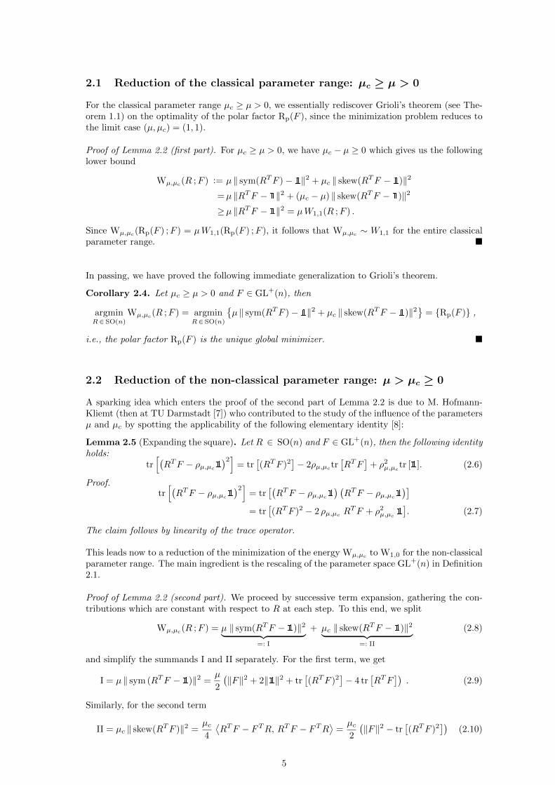
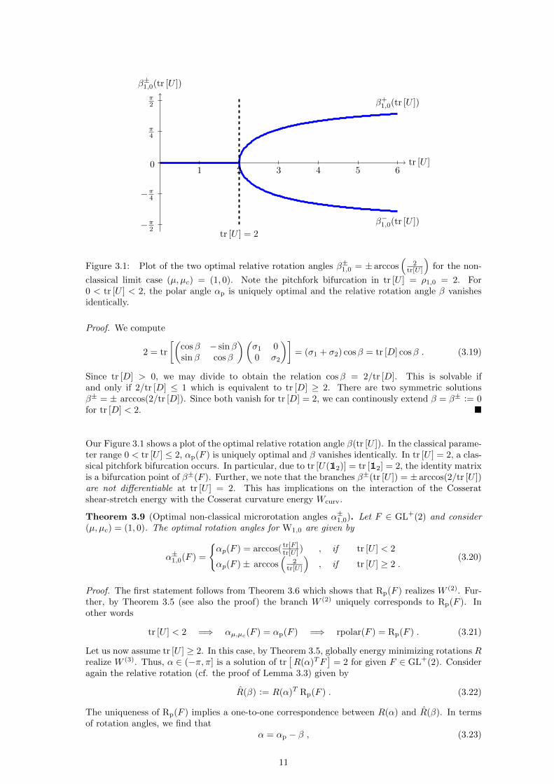
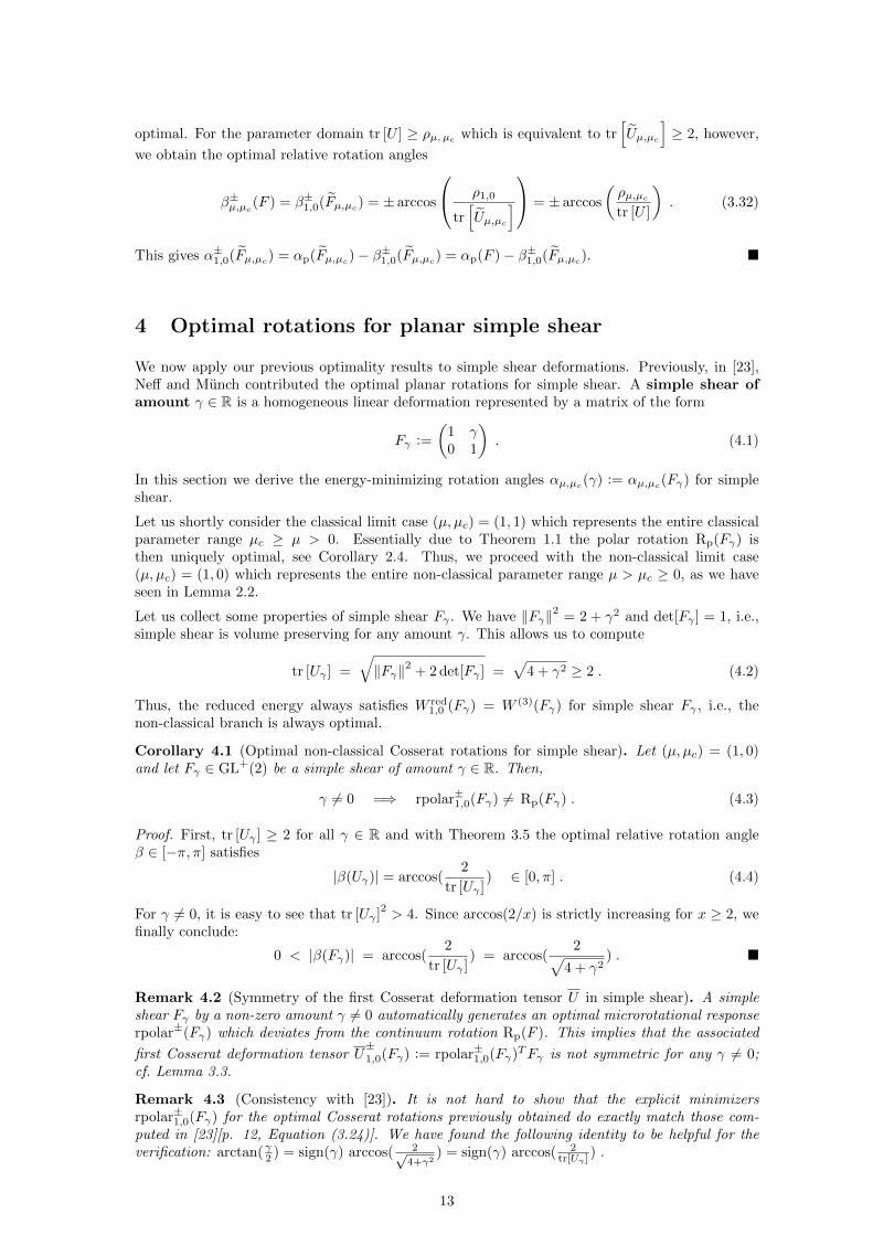
Figure 3.1: Plot of the two optimal relative rotation angles β±1,0 = ± arccos(

2tr[U ]

)for the non-

classical limit case (µ, µc) = (1, 0). Note the pitchfork bifurcation in tr [U ] = ρ1,0 = 2. For0 < tr [U ] < 2, the polar angle αp is uniquely optimal and the relative rotation angle β vanishesidentically.

Proof. We compute

2 = tr

[(cosβ − sinβsinβ cosβ

)(σ1 00 σ2

)]= (σ1 + σ2) cosβ = tr [D] cosβ . (3.19)

Since tr [D] > 0, we may divide to obtain the relation cosβ = 2/tr [D]. This is solvable ifand only if 2/tr [D] ≤ 1 which is equivalent to tr [D] ≥ 2. There are two symmetric solutionsβ± = ± arccos(2/tr [D]). Since both vanish for tr [D] = 2, we can continously extend β = β± := 0for tr [D] < 2.

Our Figure 3.1 shows a plot of the optimal relative rotation angle β(tr [U ]). In the classical parame-ter range 0 < tr [U ] ≤ 2, αp(F ) is uniquely optimal and β vanishes identically. In tr [U ] = 2, a clas-sical pitchfork bifurcation occurs. In particular, due to tr [U(12)] = tr [12] = 2, the identity matrixis a bifurcation point of β±(F ). Further, we note that the branches β±(tr [U ]) = ± arccos(2/tr [U ])are not differentiable at tr [U ] = 2. This has implications on the interaction of the Cosseratshear-stretch energy with the Cosserat curvature energy Wcurv.

Theorem 3.9 (Optimal non-classical microrotation angles α±1,0). Let F ∈ GL+(2) and consider(µ, µc) = (1, 0). The optimal rotation angles for W1,0 are given by

α±1,0(F ) =

αp(F ) = arccos( tr[F ]

tr[U ] ) , if tr [U ] < 2

αp(F )± arccos(

2tr[U ]

), if tr [U ] ≥ 2 .

(3.20)

Proof. The first statement follows from Theorem 3.6 which shows that Rp(F ) realizes W (2). Fur-ther, by Theorem 3.5 (see also the proof) the branch W (2) uniquely corresponds to Rp(F ). Inother words

tr [U ] < 2 =⇒ αµ,µc(F ) = αp(F ) =⇒ rpolar(F ) = Rp(F ) . (3.21)

Let us now assume tr [U ] ≥ 2. In this case, by Theorem 3.5, globally energy minimizing rotations Rrealize W (3). Thus, α ∈ (−π, π] is a solution of tr

[R(α)TF

]= 2 for given F ∈ GL+(2). Consider

again the relative rotation (cf. the proof of Lemma 3.3) given by

R(β) := R(α)T Rp(F ) . (3.22)

The uniqueness of Rp(F ) implies a one-to-one correspondence between R(α) and R(β). In termsof rotation angles, we find that

α = αp − β , (3.23)

11

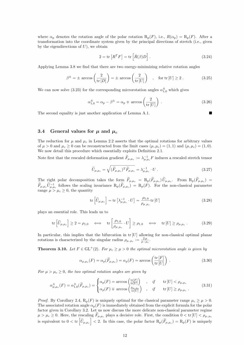
where αp denotes the rotation angle of the polar rotation Rp(F ), i.e., R(αp) = Rp(F ). After atransformation into the coordinate system given by the principal directions of stretch (i.e., givenby the eigendirections of U), we obtain

2 = tr[RTF

]= tr

[R(β)D

]. (3.24)

Applying Lemma 3.8 we find that there are two energy-minimizing relative rotation angles

β± = ± arccos

(2

tr [D]

)= ± arccos

(2

tr [U ]

), for tr [U ] ≥ 2 . (3.25)

We can now solve (3.23) for the corresponding microrotation angles α±1,0 which gives

α±1,0 = αp − β± = αp ∓ arccos

(2

tr [U ]

). (3.26)

The second equality is just another application of Lemma A.1.

3.4 General values for µ and µc

The reduction for µ and µc in Lemma 2.2 asserts that the optimal rotations for arbitrary valuesof µ > 0 and µc ≥ 0 can be reconstructed from the limit cases (µ, µc) = (1, 1) and (µ, µc) = (1, 0).We now detail this procedure which essentially exploits Definition 2.1.

Note first that the rescaled deformation gradient Fµ,µc := λ−1µ,µcF induces a rescaled stretch tensor

Uµ,µc =

√(Fµ,µc)

T Fµ,µc = λ−1µ,µc · U . (3.27)

The right polar decomposition takes the form Fµ,µc = Rp(Fµ,µc) Uµ,µc . From Rp(Fµ,µc) =

Fµ,µcU−1µ,µc follows the scaling invariance Rp(Fµ,µc) = Rp(F ). For the non-classical parameter

range µ > µc ≥ 0, the quantity

tr[Uµ,µc

]= tr

[λ−1µ,µc · U

]=

ρ1,0

ρµ,µctr [U ] (3.28)

plays an essential role. This leads us to

tr[Uµ,µc

]≥ 2 = ρ1,0 ⇐⇒ tr

[ρ1,0

ρµ,µc· U]≥ ρ1,0 ⇐⇒ tr [U ] ≥ ρµ,µc . (3.29)

In particular, this implies that the bifurcation in tr [U ] allowing for non-classical optimal planarrotations is characterized by the singular radius ρµ, µc

:= 2µµ -µc

.

Theorem 3.10. Let F ∈ GL+(2). For µc ≥ µ > 0 the optimal microrotation angle is given by

αµ,µc(F ) = αp(Fµ,µc) = αp(F ) = arccos

(tr [F ]

tr [U ]

). (3.30)

For µ > µc ≥ 0, the two optimal rotation angles are given by

α±µ,µc(F ) = α±1,0(Fµ,µc) =

αp(F ) = arccos(

tr[F ]tr[U ]

), if tr [U ] < ρµ,µc

αp(F )∓ arccos(ρµ, µctr[U ]

), if tr [U ] ≥ ρµ,µc .

(3.31)

Proof. By Corollary 2.4, Rp(F ) is uniquely optimal for the classical parameter range µc ≥ µ > 0.The associated rotation angle αp(F ) is immediately obtained from the explicit formula for the polarfactor given in Corollary 3.2. Let us now discuss the more delicate non-classical parameter regimeµ > µc ≥ 0. Here, the rescaling Fµ,µc plays a decisive role. First, the condition 0 < tr [U ] < ρµ, µc

is equivalent to 0 < tr[Uµ,µc

]< 2. In this case, the polar factor Rp(Fµ,µc) = Rp(F ) is uniquely

12

optimal. For the parameter domain tr [U ] ≥ ρµ, µcwhich is equivalent to tr

[Uµ,µc

]≥ 2, however,

we obtain the optimal relative rotation angles

β±µ,µc(F ) = β±1,0(Fµ,µc) = ± arccos

ρ1,0

tr[Uµ,µc

] = ± arccos

(ρµ,µctr [U ]

). (3.32)

This gives α±1,0(Fµ,µc) = αp(Fµ,µc)− β±1,0(Fµ,µc) = αp(F )− β±1,0(Fµ,µc).

4 Optimal rotations for planar simple shear

We now apply our previous optimality results to simple shear deformations. Previously, in [23],Neff and Munch contributed the optimal planar rotations for simple shear. A simple shear ofamount γ ∈ R is a homogeneous linear deformation represented by a matrix of the form

Fγ :=

(1 γ0 1

). (4.1)

In this section we derive the energy-minimizing rotation angles αµ,µc(γ) := αµ,µc(Fγ) for simpleshear.

Let us shortly consider the classical limit case (µ, µc) = (1, 1) which represents the entire classicalparameter range µc ≥ µ > 0. Essentially due to Theorem 1.1 the polar rotation Rp(Fγ) isthen uniquely optimal, see Corollary 2.4. Thus, we proceed with the non-classical limit case(µ, µc) = (1, 0) which represents the entire non-classical parameter range µ > µc ≥ 0, as we haveseen in Lemma 2.2.

Let us collect some properties of simple shear Fγ . We have ‖Fγ‖2 = 2 + γ2 and det[Fγ ] = 1, i.e.,simple shear is volume preserving for any amount γ. This allows us to compute

tr [Uγ ] =

√‖Fγ‖2 + 2 det[Fγ ] =

√4 + γ2 ≥ 2 . (4.2)

Thus, the reduced energy always satisfies W red1,0 (Fγ) = W (3)(Fγ) for simple shear Fγ , i.e., the

non-classical branch is always optimal.

Corollary 4.1 (Optimal non-classical Cosserat rotations for simple shear). Let (µ, µc) = (1, 0)and let Fγ ∈ GL+(2) be a simple shear of amount γ ∈ R. Then,

γ 6= 0 =⇒ rpolar±1,0(Fγ) 6= Rp(Fγ) . (4.3)

Proof. First, tr [Uγ ] ≥ 2 for all γ ∈ R and with Theorem 3.5 the optimal relative rotation angleβ ∈ [−π, π] satisfies

|β(Uγ)| = arccos(2

tr [Uγ ]) ∈ [0, π] . (4.4)

For γ 6= 0, it is easy to see that tr [Uγ ]2> 4. Since arccos(2/x) is strictly increasing for x ≥ 2, we

finally conclude:

0 < |β(Fγ)| = arccos(2

tr [Uγ ]) = arccos(

2√4 + γ2

) .

Remark 4.2 (Symmetry of the first Cosserat deformation tensor U in simple shear). A simpleshear Fγ by a non-zero amount γ 6= 0 automatically generates an optimal microrotational responserpolar±(Fγ) which deviates from the continuum rotation Rp(F ). This implies that the associated

first Cosserat deformation tensor U±1,0(Fγ) := rpolar±1,0(Fγ)TFγ is not symmetric for any γ 6= 0;

cf. Lemma 3.3.

Remark 4.3 (Consistency with [23]). It is not hard to show that the explicit minimizersrpolar±1,0(Fγ) for the optimal Cosserat rotations previously obtained do exactly match those com-puted in [23][p. 12, Equation (3.24)]. We have found the following identity to be helpful for theverification: arctan(γ2 ) = sign(γ) arccos( 2√

4+γ2) = sign(γ) arccos( 2

tr[Uγ ] ) .

13

-10 -5 5 10

20

40

60

80

100

120W (1)(Fγ)

W (2)(Fγ)

W (3)(Fγ)

γ

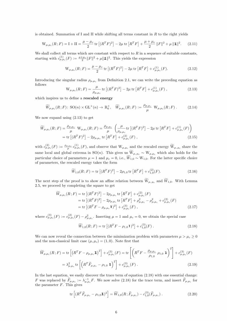
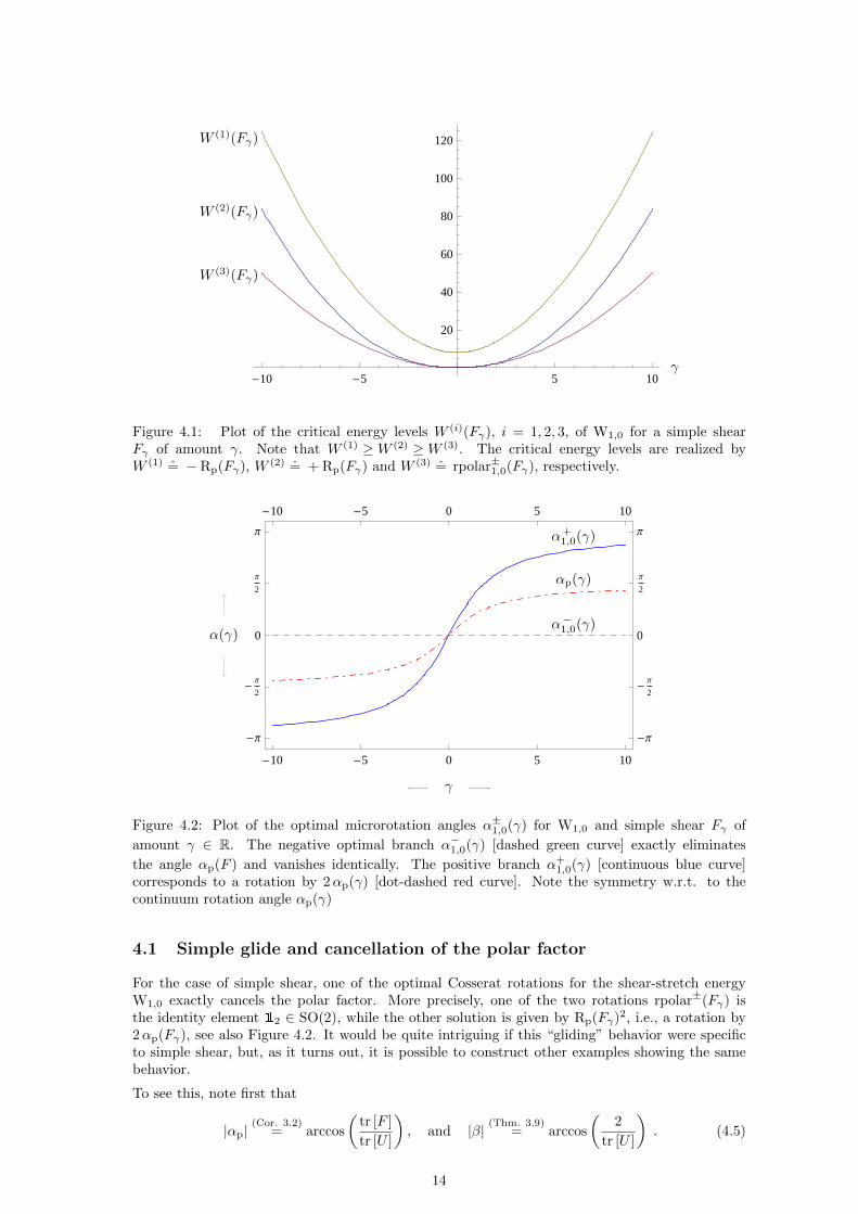
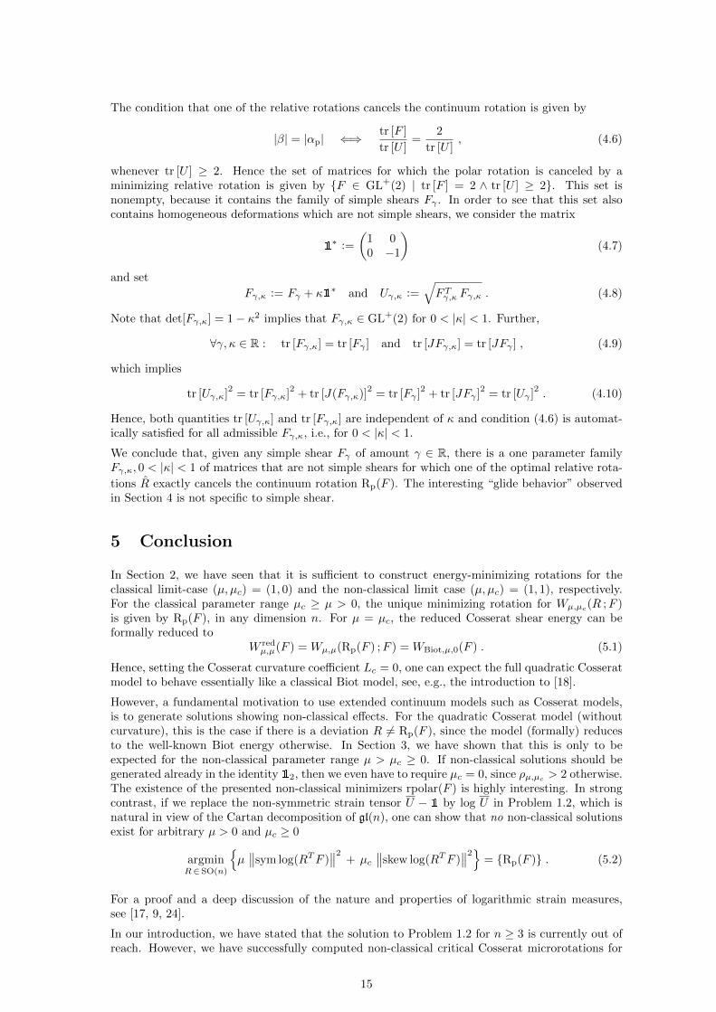
Figure 4.1: Plot of the critical energy levels W (i)(Fγ), i = 1, 2, 3, of W1,0 for a simple shearFγ of amount γ. Note that W (1) ≥W (2) ≥W (3). The critical energy levels are realized byW (1) = − Rp(Fγ), W (2) = + Rp(Fγ) and W (3) = rpolar±1,0(Fγ), respectively.

-10 -5 0 5 10

-Π

- Π

2

0

Π

2

Π

-10 -5 0 5 10

-Π

- Π

2

0

Π

2

Πα+1,0(γ)

αp(γ)

α−1,0(γ)

γ

α(γ)

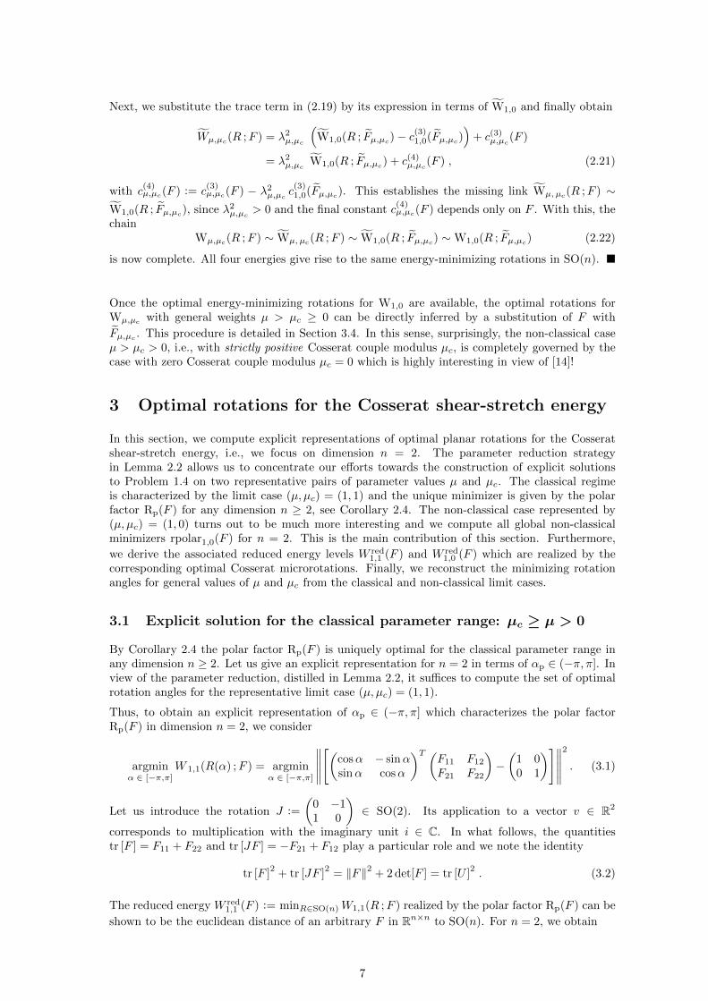
Figure 4.2: Plot of the optimal microrotation angles α±1,0(γ) for W1,0 and simple shear Fγ of

amount γ ∈ R. The negative optimal branch α−1,0(γ) [dashed green curve] exactly eliminates

the angle αp(F ) and vanishes identically. The positive branch α+1,0(γ) [continuous blue curve]

corresponds to a rotation by 2αp(γ) [dot-dashed red curve]. Note the symmetry w.r.t. to thecontinuum rotation angle αp(γ)

4.1 Simple glide and cancellation of the polar factor

For the case of simple shear, one of the optimal Cosserat rotations for the shear-stretch energyW1,0 exactly cancels the polar factor. More precisely, one of the two rotations rpolar±(Fγ) isthe identity element 12 ∈ SO(2), while the other solution is given by Rp(Fγ)2, i.e., a rotation by2αp(Fγ), see also Figure 4.2. It would be quite intriguing if this “gliding” behavior were specificto simple shear, but, as it turns out, it is possible to construct other examples showing the samebehavior.

To see this, note first that

|αp|(Cor. 3.2)

= arccos

(tr [F ]

tr [U ]

), and |β| (Thm. 3.9)

= arccos

(2

tr [U ]

). (4.5)

14

The condition that one of the relative rotations cancels the continuum rotation is given by

|β| = |αp| ⇐⇒ tr [F ]

tr [U ]=

2

tr [U ], (4.6)

whenever tr [U ] ≥ 2. Hence the set of matrices for which the polar rotation is canceled by aminimizing relative rotation is given by F ∈ GL+(2) | tr [F ] = 2 ∧ tr [U ] ≥ 2. This set isnonempty, because it contains the family of simple shears Fγ . In order to see that this set alsocontains homogeneous deformations which are not simple shears, we consider the matrix

1∗ :=

(1 00 −1

)(4.7)

and set

Fγ,κ := Fγ + κ1∗ and Uγ,κ :=√FTγ,κ Fγ,κ . (4.8)

Note that det[Fγ,κ] = 1− κ2 implies that Fγ,κ ∈ GL+(2) for 0 < |κ| < 1. Further,

∀γ, κ ∈ R : tr [Fγ,κ] = tr [Fγ ] and tr [JFγ,κ] = tr [JFγ ] , (4.9)

which implies

tr [Uγ,κ]2

= tr [Fγ,κ]2

+ tr [J(Fγ,κ)]2

= tr [Fγ ]2

+ tr [JFγ ]2

= tr [Uγ ]2. (4.10)

Hence, both quantities tr [Uγ,κ] and tr [Fγ,κ] are independent of κ and condition (4.6) is automat-ically satisfied for all admissible Fγ,κ, i.e., for 0 < |κ| < 1.

We conclude that, given any simple shear Fγ of amount γ ∈ R, there is a one parameter familyFγ,κ, 0 < |κ| < 1 of matrices that are not simple shears for which one of the optimal relative rota-

tions R exactly cancels the continuum rotation Rp(F ). The interesting “glide behavior” observedin Section 4 is not specific to simple shear.

5 Conclusion

In Section 2, we have seen that it is sufficient to construct energy-minimizing rotations for theclassical limit-case (µ, µc) = (1, 0) and the non-classical limit case (µ, µc) = (1, 1), respectively.For the classical parameter range µc ≥ µ > 0, the unique minimizing rotation for Wµ,µc(R ;F )is given by Rp(F ), in any dimension n. For µ = µc, the reduced Cosserat shear energy can beformally reduced to

W redµ,µ(F ) = Wµ,µ(Rp(F ) ;F ) = WBiot,µ,0(F ) . (5.1)

Hence, setting the Cosserat curvature coefficient Lc = 0, one can expect the full quadratic Cosseratmodel to behave essentially like a classical Biot model, see, e.g., the introduction to [18].

However, a fundamental motivation to use extended continuum models such as Cosserat models,is to generate solutions showing non-classical effects. For the quadratic Cosserat model (withoutcurvature), this is the case if there is a deviation R 6= Rp(F ), since the model (formally) reducesto the well-known Biot energy otherwise. In Section 3, we have shown that this is only to beexpected for the non-classical parameter range µ > µc ≥ 0. If non-classical solutions should begenerated already in the identity 12, then we even have to require µc = 0, since ρµ,µc > 2 otherwise.The existence of the presented non-classical minimizers rpolar(F ) is highly interesting. In strongcontrast, if we replace the non-symmetric strain tensor U − 1 by log U in Problem 1.2, which isnatural in view of the Cartan decomposition of gl(n), one can show that no non-classical solutionsexist for arbitrary µ > 0 and µc ≥ 0

argminR∈ SO(n)

µ∥∥sym log(RTF )

∥∥2+ µc

∥∥skew log(RTF )∥∥2

= Rp(F ) . (5.2)

For a proof and a deep discussion of the nature and properties of logarithmic strain measures,see [17, 9, 24].

In our introduction, we have stated that the solution to Problem 1.2 for n ≥ 3 is currently out ofreach. However, we have successfully computed non-classical critical Cosserat microrotations for

15

n = 3 using a parametrisation by unit quaternions and computational algebra. Further, we havemanaged to select the energy minimal branches, experimentally. An extensive numerical validationshows, moreover, that our candidates are very likely the global minimizers. The mechanismsdiscovered for the case n = 2 in the present work do carry over to the case n = 3 quite literally upto the determination of the microrotation axis. This is the content of a forthcoming second partof this paper [5]. For dimensions n > 3, the weighted Problem 1.2 is, to the best of our knowledge,still completely open. It seems to us, however, reasonable to guess that a transformation into theprincipal directions of stretch, i.e., the eigendirections of U , is a good plan of attack.

Remark 5.1 (Final Conclusion). To ascertain the complete absence of a non-classical responsewithin a geometrically nonlinear quadratic Cosserat-micropolar shear-stretch energy, one mustchoose a classical parameter set, i.e., µc ≥ µ > 0.

References

[1] M. Bırsan and P. Neff. Existence of minimizers in the geometrically non-linear 6-parameter resultant shell theory with drilling rotations. Math. Mech. Solids, DOI:10.1177/1081286512466659, 2013. 2

[2] C. G. Boehmer, P. Neff, and B. Seymenoglu. Soliton-like solutions based on geometricallynonlinear Cosserat micropolar elasticity. arXiv preprint arXiv:1503.08860, 2015. 2

[3] C. Bouby, D. Fortune, W. Pietraszkiewicz, and C. Vallee. Direct determination of the rotationin the polar decomposition of the deformation gradient by maximizing a Rayleigh quotient.Z. Angew. Math. Mech., 85:155–162, 2005. 2

[4] V. A. Eremeyev, L. P. Lebedev, and H. Altenbach. Foundations of micropolar mechanics.Springer, 2012. 2

[5] A. Fischle and P. Neff. The geometrically nonlinear Cosserat micropolar shear-stretch en-ergy. Part II: Non-classical energy-minimizing microrotations in 3D and their experimentalvalidation. in preparation, 2015. 16

[6] G. Grioli. Una proprieta di minimo nella cinematica delle deformazioni finite. Boll. Un. Math.Ital., 2:252–255, 1940. 2

[7] M. Hofmann-Kliemt. The Invariant Complex Structure on the Homogeneous SpaceDiff(S1)/Rot(S1). PhD thesis, TU Darmstadt, July 2007. 5

[8] M. Hofmann-Kliemt. On parameter reduction. (personal communication), 2007. 5

[9] J. Lankeit, P. Neff, and Y. Nakatsukasa. The minimization of matrix logarithms: On afundamental property of the unitary polar factor. Lin. Alg. Appl., 449:28–42, 2014. 15

[10] J. Lankeit, P. Neff, and F. Osterbrink. Integrability conditions between the first and secondCosserat deformation tensor in geometrically nonlinear micropolar models and existence ofminimizers. arXiv preprint arXiv:1504.08003, 2015. 2

[11] R. J. Martin, I.-D. Ghiba, and P. Neff. Rank-one convexity implies polyconvexity forisotropic, objective and isochoric elastic energies in the two-dimensional case. arXiv preprintarXiv:1507.00266, 2015. 8

[12] L.C. Martins and P. Podio-Guidugli. An elementary proof of the polar decomposition theorem.Amer. Math. Month., 87:288–290, 1980. 2

[13] P. Neff. Finite multiplicative plasticity for small elastic strains with linear balance equationsand grain boundary relaxation. Cont. Mech. Thermod., 15(2):161–195, 2003. 2

[14] P. Neff. The Cosserat couple modulus for continuous solids is zero viz the linearized Cauchy-stress tensor is symmetric. Z. Angew. Math. Mech., 86:892–912, 2006. 2, 4, 7

[15] P. Neff. A finite-strain elastic-plastic Cosserat theory for polycrystals with grain rotations.Int. J. Engng. Sci., 44:574–594, 2006. 2

16

[16] P. Neff, M. Bırsan, and F. Osterbrink. Existence theorem for geometrically nonlinear Cosseratmicropolar model under uniform convexity requirements. J. Elasticity, pages 1–23, 2015. 2

[17] P. Neff, B. Eidel, and R. J. Martin. Geometry of logarithmic strain measures in solid mechan-ics. arXiv preprint arXiv:1505.02203, 2015. 15

[18] P. Neff, A. Fischle, and I. Munch. Symmetric Cauchy-stresses do not imply symmetric Biot-strains in weak formulations of isotropic hyperelasticity with rotational degrees of freedom.Acta Mech., 197:19–30, 2008. 2, 8, 9, 15

[19] P. Neff and J. Jeong. A new paradigm: the linear isotropic Cosserat model with conformallyinvariant curvature energy. Z. Angew. Math. Mech., 89(2):107–122, 2009. 2

[20] P. Neff, J. Jeong, and A. Fischle. Stable identification of linear isotropic Cosserat parameters:bounded stiffness in bending and torsion implies conformal invariance of curvature. ActaMech., 211(3-4):237–249, 2010. 2

[21] P. Neff, J. Lankeit, and A. Madeo. On Grioli’s minimum property and its relation to Cauchy’spolar decomposition. Int. J. Engng. Sci., 80:209–217, 2014. 2

[22] P. Neff and I. Munch. Curl bounds Grad on SO(3). ESAIM: COCV, 14(1):148–159, 2008. 2

[23] P. Neff and I. Munch. Simple shear in nonlinear Cosserat elasticity: bifurcation and inducedmicrostructure. Cont. Mech. Thermod., 21(3):195–221, 2009. 13

[24] P. Neff, Y. Nakatsukasa, and A. Fischle. A logarithmic minimization property of the unitarypolar factor in the spectral and Frobenius norms. SIAM J. Matrix Anal. Appl., 35(3):1132–1154, 2014. 15

[25] W. Pietraszkiewicz and V. A. Eremeyev. On vectorially parameterized natural strain measuresof the non-linear Cosserat continuum. Int. J. Solids Struct., 46(11):2477–2480, 2009. 2

[26] C. Sansour and S. Skatulla. A non-linear Cosserat continuum-based formulation and movingleast square approximations in computations of size-scale effects in elasticity. Comp. Mat.Sci., 41(4):589–601, 2008. 2

[27] K. Wisniewski. A shell theory with independent rotations for relaxed Biot stress and rightstrain. Comp. Mech., 21(2):101–122, 1998. 2

[28] K. Wisniewski and E. Turska. Kinematics of finite rotation shells with in-plane twist param-eter. Comp. Meth. Appl. Mech. Engng., 190:1117–1135, 2000. 2

[29] K. Wisniewski and E. Turska. Second-order shell kinematics implied by rotation constraint-equation. J. Elasticity, 67:229–246, 2002. 2

A Appendix

A.1 Some planar matrix identities for U and F

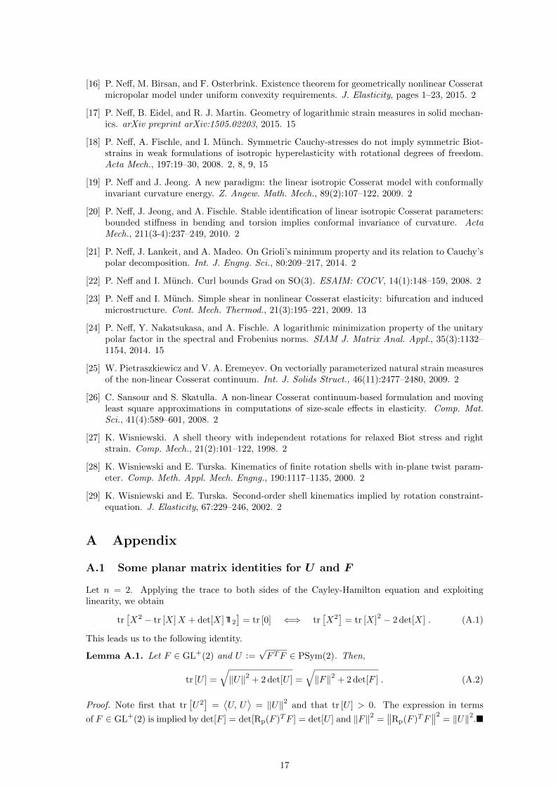
Let n = 2. Applying the trace to both sides of the Cayley-Hamilton equation and exploitinglinearity, we obtain

tr[X2 − tr [X]X + det[X]12

]= tr [0] ⇐⇒ tr

[X2]

= tr [X]2 − 2 det[X] . (A.1)

This leads us to the following identity.

Lemma A.1. Let F ∈ GL+(2) and U :=√FTF ∈ PSym(2). Then,

tr [U ] =

√‖U‖2 + 2 det[U ] =

√‖F‖2 + 2 det[F ] . (A.2)

Proof. Note first that tr[U2]

=⟨U, U

⟩= ‖U‖2 and that tr [U ] > 0. The expression in terms

of F ∈ GL+(2) is implied by det[F ] = det[Rp(F )TF ] = det[U ] and ‖F‖2 =∥∥Rp(F )TF

∥∥2= ‖U‖2.

17