
Measurement of jets production in association with a Z ...hss.ulb.uni-bonn.de/2013/3130/3130.pdf ·...
151
Universität Bonn Physikalisches Institut Measurement of jets production in association with a Z boson and in the search for the SM Higgs boson via H → ττ → ‘‘ + 4ν with ATLAS Serena Psoroulas Three measurements focussing on the understanding of jet final states in ATLAS, in di-jet, Z and Higgs boson candidate events, using data corresponding to an integrated luminosity of 35 pb -1 in 2010 and 4.7 fb -1 in 2011, are presented. In the first part, a calibration method, based on the transverse momentum balance in di-jet events, is described. The method is used to estimate the uncertainty of the jet energy scale in the forward region. The results show that the parton shower models are limited in reproducing the results in data, mostly for jets of low transverse momentum. In the second part, the differential cross section measurement of the Z → ‘‘ + jets process is reported. Phase space regions not been previously studied at other experiments are investigated. The models used for the theory predictions provide a good description of the data, within the relative uncertainties. In the last part, two contribution to the Higgs searches in the H → ττ channel are shown: the modelling of the Z → ττ background, and the modelling of jet final states. The Z → ττ background is derived from data and validated in the H → ττ → ‘‘ + 4ν channel. The modelling of jet final states in simulations is in good agreement with the data, when low-energy pile-up effects are subtracted. Physikalisches Institut der Universität Bonn Nußallee 12 D-53115 Bonn BONN-IR-2012-11 Oktober 2012 ISSN-0172-8741
-
Upload
trinhkhanh -
Category
Documents
-
view
216 -
download
0
Transcript of Measurement of jets production in association with a Z ...hss.ulb.uni-bonn.de/2013/3130/3130.pdf ·...
Universität BonnPhysikalisches Institut
Measurement of jets production in association
with a Z boson and in the search for the SM
Higgs boson via H → ττ→ ``+ 4ν with ATLAS
Serena Psoroulas
Three measurements focussing on the understanding of jet final states in ATLAS, in di-jet, Z andHiggs boson candidate events, using data corresponding to an integrated luminosity of 35 pb−1 in2010 and 4.7 fb−1 in 2011, are presented.In the first part, a calibration method, based on the transverse momentum balance in di-jet events,is described. The method is used to estimate the uncertainty of the jet energy scale in the forwardregion. The results show that the parton shower models are limited in reproducing the results indata, mostly for jets of low transverse momentum.In the second part, the differential cross section measurement of the Z → `` + jets process isreported. Phase space regions not been previously studied at other experiments are investigated.The models used for the theory predictions provide a good description of the data, within therelative uncertainties.In the last part, two contribution to the Higgs searches in the H → ττ channel are shown: themodelling of the Z → ττ background, and the modelling of jet final states. The Z → ττ backgroundis derived from data and validated in the H → ττ → `` + 4ν channel. The modelling of jetfinal states in simulations is in good agreement with the data, when low-energy pile-up effects aresubtracted.
Physikalisches Institut derUniversität BonnNußallee 12D-53115 Bonn
BONN-IR-2012-11Oktober 2012ISSN-0172-8741

Universität BonnPhysikalisches Institut
Measurement of jets production in associationwith a Z boson and in the search for the SM
Higgs boson via H → ττ→ ``+ 4ν with ATLAS
Serena Psoroulasaus
Rom, Italien
Dieser Forschungsbericht wurde als Dissertation von der Mathematisch-NaturwissenschaftlichenFakultät der Universität Bonn angenommen und ist 2013 auf dem Hochschulschriftenserver derULB Bonn http://hss.ulb.uni-bonn.de/diss_online elektronisch publiziert.
1. Gutachter: Prof. Dr. Norbert Wermes2. Gutachter: Prof. Dr. Klaus Desch
Angenommen am: 24.08.2012Tag der Promotion: 28.09.2012

Contents
1 Introduction 1
2 Theory predictions for physics at the LHC 52.1 The Standard Model of Particle Physics . . . . . . . . . . . . . . . . . . . . . . . . . . . . . 5
2.1.1 The Higgs mechanism . . . . . . . . . . . . . . . . . . . . . . . . . . . . . . . . . . . 72.2 QCD at high energy colliders . . . . . . . . . . . . . . . . . . . . . . . . . . . . . . . . . . . 8
2.2.1 The parton model of QCD . . . . . . . . . . . . . . . . . . . . . . . . . . . . . . . . 92.2.2 QCD properties and jets . . . . . . . . . . . . . . . . . . . . . . . . . . . . . . . . . 102.2.3 Parton shower models . . . . . . . . . . . . . . . . . . . . . . . . . . . . . . . . . . . 11
2.3 Z boson production in association with jets . . . . . . . . . . . . . . . . . . . . . . . . . . 132.4 Higgs boson production at LHC . . . . . . . . . . . . . . . . . . . . . . . . . . . . . . . . . 14
2.4.1 Production and decay channels . . . . . . . . . . . . . . . . . . . . . . . . . . . . . 152.4.2 H → ττ decay channel . . . . . . . . . . . . . . . . . . . . . . . . . . . . . . . . . . 152.4.3 Z boson as a background for H → ττ searches . . . . . . . . . . . . . . . . . . . 182.4.4 Theoretical uncertainties on Higgs cross sections . . . . . . . . . . . . . . . . . . 19
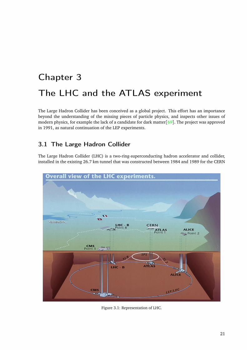
3 The LHC and the ATLAS experiment 213.1 The Large Hadron Collider . . . . . . . . . . . . . . . . . . . . . . . . . . . . . . . . . . . . 21
3.1.1 Pile-up . . . . . . . . . . . . . . . . . . . . . . . . . . . . . . . . . . . . . . . . . . . . 233.2 The ATLAS detector . . . . . . . . . . . . . . . . . . . . . . . . . . . . . . . . . . . . . . . . . 25
3.2.1 Overall detector . . . . . . . . . . . . . . . . . . . . . . . . . . . . . . . . . . . . . . 253.2.2 Coordinate system and conventions . . . . . . . . . . . . . . . . . . . . . . . . . . 263.2.3 Inner Detector (Tracker) . . . . . . . . . . . . . . . . . . . . . . . . . . . . . . . . . 263.2.4 The LAr Calorimeter . . . . . . . . . . . . . . . . . . . . . . . . . . . . . . . . . . . . 283.2.5 Hadron calorimeter . . . . . . . . . . . . . . . . . . . . . . . . . . . . . . . . . . . . 293.2.6 Muon Spectrometer . . . . . . . . . . . . . . . . . . . . . . . . . . . . . . . . . . . . 323.2.7 Trigger and Data Acquisition System . . . . . . . . . . . . . . . . . . . . . . . . . . 323.2.8 Simulation of the ATLAS detector . . . . . . . . . . . . . . . . . . . . . . . . . . . . 33
4 Jet Algorithms in VBF Higgs searches 354.1 What is a jet? . . . . . . . . . . . . . . . . . . . . . . . . . . . . . . . . . . . . . . . . . . . . . 354.2 Jet reconstruction in ATLAS . . . . . . . . . . . . . . . . . . . . . . . . . . . . . . . . . . . . 39
4.2.1 Input to jet reconstruction . . . . . . . . . . . . . . . . . . . . . . . . . . . . . . . . 394.3 Jet Algorithm studies in Vector-Boson-Fusion simulated samples . . . . . . . . . . . . . 40
4.3.1 Motivation . . . . . . . . . . . . . . . . . . . . . . . . . . . . . . . . . . . . . . . . . . 404.3.2 Analysis details . . . . . . . . . . . . . . . . . . . . . . . . . . . . . . . . . . . . . . . 424.3.3 Comparison of algorithms without pile-up . . . . . . . . . . . . . . . . . . . . . . 444.3.4 Comparison of algorithms with pile-up . . . . . . . . . . . . . . . . . . . . . . . . 49
4.4 Conclusions . . . . . . . . . . . . . . . . . . . . . . . . . . . . . . . . . . . . . . . . . . . . . . 49
i
5 Jet η-intercalibration in 2010 data atp
s = 7 TeV 515.1 Strategy . . . . . . . . . . . . . . . . . . . . . . . . . . . . . . . . . . . . . . . . . . . . . . . . 515.2 Jet energy scale calibration . . . . . . . . . . . . . . . . . . . . . . . . . . . . . . . . . . . . 52
5.2.1 Hadronic showers in a calorimeter . . . . . . . . . . . . . . . . . . . . . . . . . . . 525.2.2 ATLAS calibration schemes . . . . . . . . . . . . . . . . . . . . . . . . . . . . . . . . 54
5.3 In-situ η-intercalibration of the ATLAS detector using di-jet events . . . . . . . . . . . 585.3.1 Methods used in this analysis . . . . . . . . . . . . . . . . . . . . . . . . . . . . . . 585.3.2 Data and Monte Carlo samples . . . . . . . . . . . . . . . . . . . . . . . . . . . . . 615.3.3 Di-jet events reconstruction and selection . . . . . . . . . . . . . . . . . . . . . . . 625.3.4 Results . . . . . . . . . . . . . . . . . . . . . . . . . . . . . . . . . . . . . . . . . . . . 63
5.4 Outlook . . . . . . . . . . . . . . . . . . . . . . . . . . . . . . . . . . . . . . . . . . . . . . . . 67
6 Measurement of the production cross section for Z/γ∗ in association with jets 716.1 Data and simulation samples . . . . . . . . . . . . . . . . . . . . . . . . . . . . . . . . . . . 736.2 Z → `` + jets selection . . . . . . . . . . . . . . . . . . . . . . . . . . . . . . . . . . . . . . . 746.3 Detector level results . . . . . . . . . . . . . . . . . . . . . . . . . . . . . . . . . . . . . . . . 78
6.3.1 Detector level validation . . . . . . . . . . . . . . . . . . . . . . . . . . . . . . . . . 786.3.2 Jet differential distributions . . . . . . . . . . . . . . . . . . . . . . . . . . . . . . . 80
6.4 Comparison with Monte Carlo LO and NLO pQCD predictions . . . . . . . . . . . . . . 816.4.1 Jet systematic uncertainties . . . . . . . . . . . . . . . . . . . . . . . . . . . . . . . 816.4.2 Unfolding of detector results . . . . . . . . . . . . . . . . . . . . . . . . . . . . . . . 866.4.3 Combination of electron and muon channel . . . . . . . . . . . . . . . . . . . . . 88
6.5 Outlook . . . . . . . . . . . . . . . . . . . . . . . . . . . . . . . . . . . . . . . . . . . . . . . . 89
7 Search for the Standard Model Higgs boson in the τ+τ− channel 957.1 Strategy . . . . . . . . . . . . . . . . . . . . . . . . . . . . . . . . . . . . . . . . . . . . . . . . 957.2 Definition of analysis categories . . . . . . . . . . . . . . . . . . . . . . . . . . . . . . . . . 97
7.2.1 Jet topology in Higgs production channels . . . . . . . . . . . . . . . . . . . . . . 977.2.2 Perturbative uncertainties in jet categories . . . . . . . . . . . . . . . . . . . . . . 987.2.3 Definition of jet categories in the 2011 analysis . . . . . . . . . . . . . . . . . . . 100
7.3 Data and simulated samples . . . . . . . . . . . . . . . . . . . . . . . . . . . . . . . . . . . 1017.4 Selection and reconstruction of physics objects . . . . . . . . . . . . . . . . . . . . . . . . 103
7.4.1 Validation of the preselection in Z → `` + jets events . . . . . . . . . . . . . . . 1047.5 Event selection . . . . . . . . . . . . . . . . . . . . . . . . . . . . . . . . . . . . . . . . . . . . 1107.6 Data-Driven Background Estimation . . . . . . . . . . . . . . . . . . . . . . . . . . . . . . 116
7.6.1 Z → ττ data-driven estimation: embedding method . . . . . . . . . . . . . . . . 1187.6.2 Validation of embedded Z → ττ events in the H → ττ→ ``+ 4ν analysis . . 121
7.7 Systematic uncertainties . . . . . . . . . . . . . . . . . . . . . . . . . . . . . . . . . . . . . . 1227.8 Results . . . . . . . . . . . . . . . . . . . . . . . . . . . . . . . . . . . . . . . . . . . . . . . . . 1257.9 Outlook . . . . . . . . . . . . . . . . . . . . . . . . . . . . . . . . . . . . . . . . . . . . . . . . 126
8 Outlook 129
Bibliography 131
List of Figures 139
List of Tables 143
ii
Chapter 1
Introduction
The main reason for the LHC physics program is the understanding of the mechanism of the Elec-troweak symmetry breaking. The Electroweak theory does not allow a mechanism to give to eachparticle its own mass. This is a fundamental problem, as not only we observe that particles do havemass, but the value of the masses of the force carriers influences the strength of the relevant force.The solution to this problem was provided by several authors [61, 70, 73–75, 82]. They showedthat, if in nature an additional scalar field exists, with the characteristics of a non-zero vacuumexpectation value, a spontaneous breaking of the Electroweak symmetry can occur. This spontan-eous breaking gives a mass to the weak bosons, in such a way that the Electromagnetic and Weakinteraction we experience is restored. The interactions of the fermions with this field also providesthem with their masses. The breaking also produces a scalar boson, the Higgs boson.
This model explains the Electroweak symmetry breaking, but introduces an additional field, thatdepends on two fundamental parameters: the Higgs mass and the non-zero expectation value ofthe field. Because those parameters enter in the definition of the electroweak masses, it is possibleto constrain them. The vacuum expectation value can be constrained with high precision using themeasurement of the Fermi constant GF : from this we obtain a value of 246 GeV. The Higgs mass,instead, can be constrained only from the radiative corrections to the top and the W boson masses.The constraints are loose in this case, predicting the Higgs mass to be around 100 GeV. From otherconstraints, for example the breaking of the unitarity at 1 TeV that would occur in WW scattering,we can expect the Higgs mass to be smaller than this value.
A “light” Higgs boson, i.e. a boson whose mass would be ≤ 200 GeV, is the favoured optionconsidering the results of the electroweak fits, that include results from the previous generation ofcolliders[38]. For this reason, low-mass Higgs searches were carried out at the LEP and Tevatronexperiments; but no evidence for the Higgs had been found in those searches.
The LHC was built to fully explore the mass range allowed by the unitarity constraint. A largeeffort has been directed towards the low-mass region, and this thesis is part of that effort. Thelatest results from ATLAS, that culminated with the discovery of a new particle consistent with thepredictions for the Standard Model (SM) Higgs boson [21], are the outcome of this long processof preparatory studies. The discovery of a new particle in this energy regime will provide theinformations we are missing to fully understand the SM, with possible consequences concerningcosmology as well. The consequences of this discovery go beyond the field of particle physics,involving all the studies about the origin and the fundamental behaviour of the universe.
The LHC explores an energy range not available at an accelerator before, and can deliver col-lisions at an incredibly high luminosity. Both features, however, require unprecedented precisionboth from the point of view of the operations, and from the point of view of the analysis. Studyingphysics at a new energy requires first of all the understanding of the physics at that energy. Thisis can be a difficult task: the models used are never perfect, and often tuned on some processesor energy ranges that don’t ensure their reliability after an extrapolation to another regime. The
1
Chapter 1 Introduction
solutions to the issue might come either from tuning some parameters of the model, or from big-ger changes to the model itself, that exploit the better understanding of the processes provided bythe new measurements. The first task of the LHC experiments has been, thus, the measurementof known SM processes. In such processes, the reliability of the tools used by the analyses - themodelling of physics objects first, and then of fundamental interactions in pp collisions - has beentested.
Outline In this thesis, study on simulated data and three measurements, performed at the ATLASexperiment using the data from the first two runs, corresponding to an integrated luminosity of35 pb−1 in 2010 and 4.7 fb−1 in 2011, are reported. The studies focusses on two topics: theunderstanding of Quantumchromodynamics (QCD) processes at the LHC, and the search for a lightHiggs boson.
QCD is the theory that describes the interaction of hadronic particles. QCD processes are do-minant in pp collisions; and because of their high cross section, the sample collected in 2010 islarge enough to investigate them. Also, they are among the largest background for Higgs and newPhysics searches: for this reason, they must be understood with a high precision.
In the context of the Higgs boson searches, I have focussed on the H → ττ channel. This is apromising channel, because it provides a clean signature (provided that the τ leptons can be wellreconstructed in the detector). The H → ττ analysis relies on the excellent performance of thedetector. The decay products are detected either in the tracking system (electrons, muons) or inthe calorimeters (electrons, hadronic taus), while the contribution from the neutrinos is estimatedfrom the missing transverse energy of the event (Emiss
T ). The sensitivity relies on a precise predictionof the signal process as well as of the large background processes. Investigating the presence ofadditional jets (a bunch of hadronic particles; see Chap. 4) in the event, is useful to separate signaland background, and enhance the sensitivity. This stresses, again, the importance of understandingthe hadronic interactions at the LHC energies, that had a central role in my whole thesis project.
Jet algorithms studies in the context of the Higgs searches The investigation of the Higgsboson production exploiting the jet characteristics started as a proof of principle in Aad et al.[9].That work investigated the possibility to extract the signal from the LHC data at 14 TeV. Sincethat publication, new technical development in the field of jet algorithms made more reconstructionalgorithms available “on the market”. A complete investigation has been carried on in all ATLASanalyses, to find the algorithm with the best performance. I have performed this study within theH → ττ analysis, and the results are reported in Chap. 4. From this and other results, the defaultATLAS algorithm has been replaced.
Jet studies in ATLAS: calibration and uncertainties During 2010, I have focussed on QCDunderstanding. I have first studied the performance of jet reconstruction in real collisions. Becausethere is no way to fully detect the energy deposited by hadronic particles in the detectors, weneed to define a reference for the energy of a jet. The ATLAS calibration uses a reference fromsimulations; looking at the deviations between several simulation models and the measurements,it’s possible to establish the precision of the calibration. This analysis, reported in Chap. 5, is afundamental first step towards a successful physics program in ATLAS.
Measurement of the production cross section for Z/γ∗ in association with jets Studyingthe production of Z bosons in association with jets is an important step in the understanding of
2
the underlying mechanisms of QCD. Also, the Z is an important background for the H → ττ decaychannel, because it can lead to the same final state: the Higgs signal will show up as a smallexcess of events on the tail of the Z resonance. I have focussed on this process in 2010, and themeasurement of the differential cross section is reported in Chap. 6. This measurement provides thelargest coverage in the phase space with respect to previous studies at hadronic colliders. My workhas investigated the possibility to expand the rapidity reach of the measurement; the previousexperience developed in the context of jet algorithms and calibration has been fundamental inreaching this goal. In addition, the measurement has investigated many variables that are importantin a Higgs analysis, as the Z → `` + jets process can provide a clean control region for the H → ττchannel.
Search for the standard model Higgs boson in the H → ττ→ ``+4ν channel Finally, theresults of the search for the Higgs boson in the H → ττ→ ``+ 4ν decay channel are presented in7. In addition to the investigation of the Z → `` + jets background, an investigation of the Z → ττbackground is performed. This is the main irreducible background to the H → ττ process. Also, itprovides additional challenges with respect to the Z → `` + jets background, due to the presenceof the missing momentum carried away by the neutrinos in the τ decay. After summarizing thestudies performed in the context of this search, the final limits on the production of the Higgsboson, presented as a ratio of the excluded cross section over the cross section predicted by theStandard Model, are shown.
Public results All the results obtained with ATLAS collisions data reported here have been pub-lished. The results on the jet calibration and uncertainties have been published in Aad et al. [10].The measurement of the Z → `` + jets cross section is published in Aad et al. [17]. The results ofthe search for the Higgs boson in the H → ττ channel have been submitted to JHEP; the preprintis public at http://arxiv.org/abs/1206.5971v1.
3


Chapter 2
Theory predictions for physics at the LHC
2.1 The Standard Model of Particle Physics
The current model of Particle Physics is known as the Standard Model (SM). It consists of a relativ-istic quantum field theory that includes all known forces of nature except gravity, since the latteris too weak at the energy scales typical for the other forces. The other forces are the Strong force,responsible for the structure of protons, neutrons and nuclei; the Electromagnetic force, that de-scribes the interaction between electric charges; and the Weak force, that describes phenomena likethe β decay. According to the SM, the Universe is composed of elementary particles, that interactvia one or more of the mentioned forces. In the theory, particles are described as fermion fields,and are divided into leptons (particles that don’t feel the strong interaction) and quarks (particlesthat feel all interactions). Interactions can occur among these fermions, mediated via vector bosonparticles. A summary of all the particles described in the SM is shown in Fig. 2.1.
Figure 2.1: Scheme showing the elementary particles described in the Standard Model.
Quarks have been considered as elementary particles since the discovery of proton substructure.To reproduce the spins and charges of the known particles, each quark carries a fractional chargeand is half-integer spin. Baryons, like the proton, are made of 3 valence quarks, while mesons, likethe pion, are made of a quark-antiquark valence pair. The valence quarks determine the particle’squantum numbers, but the actual composition of the particle is only known on a statistical basis(see Sect. 2.2.1 for the proton case). Colour symmetry is responsible for the anti-symmetric prop-erty of the wave function: the quarks have an additional quantum number that represents their
5
Chapter 2 Theory predictions for physics at the LHC
behaviour under this symmetry. The colour symmetry is an exact symmetry, represented by theSU(3) symmetry group, and the generators for this group provide the mathematical form for theforce carriers, the gluons. Gluons are massless neutral particles responsible only for the colourinteraction. Because of the non-abelian nature of the symmetry, gluons interact not only with thequarks but also among themselves. The behaviour of quarks and gluons is described by Quan-tumchromodynamics (QCD); further comments on QCD, relevant for the analysis reported in thisthesis, are in Sect. 2.2.
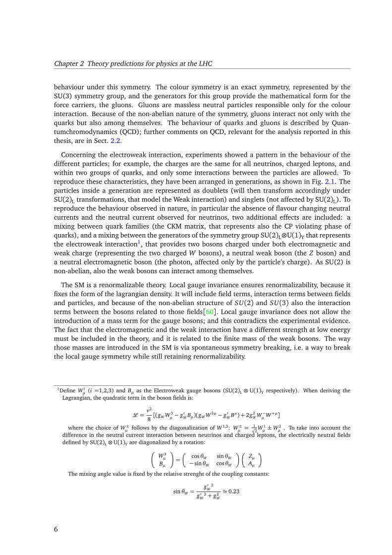
Concerning the electroweak interaction, experiments showed a pattern in the behaviour of thedifferent particles; for example, the charges are the same for all neutrinos, charged leptons, andwithin two groups of quarks, and only some interactions between the particles are allowed. Toreproduce these characteristics, they have been arranged in generations, as shown in Fig. 2.1. Theparticles inside a generation are represented as doublets (will then transform accordingly underSU(2)L transformations, that model the Weak interaction) and singlets (not affected by SU(2)L). Toreproduce the behaviour observed in nature, in particular the absence of flavour changing neutralcurrents and the neutral current observed for neutrinos, two additional effects are included: amixing between quark families (the CKM matrix, that represents also the CP violating phase ofquarks), and a mixing between the generators of the symmetry group SU(2)L⊗U(1)Y that representsthe electroweak interaction1, that provides two bosons charged under both electromagnetic andweak charge (representing the two charged W bosons), a neutral weak boson (the Z boson) anda neutral electromagnetic boson (the photon, affected only by the particle’s charge). As SU(2) isnon-abelian, also the weak bosons can interact among themselves.
The SM is a renormalizable theory. Local gauge invariance ensures renormalizability, because itfixes the form of the lagrangian density. It will include field terms, interaction terms between fieldsand particles, and because of the non-abelian structure of SU(2) and SU(3) also the interactionterms between the bosons related to those fields[60]. Local gauge invariance does not allow theintroduction of a mass term for the gauge bosons; and this contradicts the experimental evidence.The fact that the electromagnetic and the weak interaction have a different strength at low energymust be included in the theory, and it is related to the finite mass of the weak bosons. The waythose masses are introduced in the SM is via spontaneous symmetry breaking, i.e. a way to breakthe local gauge symmetry while still retaining renormalizability.
1Define W iµ (i =1,2,3) and Bµ as the Electroweak gauge bosons (SU(2)L ⊗ U(1)Y respectively). When deriving the
Lagrangian, the quadratic term in the boson fields is:
L =v2
8[(gW W 3
µ− g ′W Bµ)(gW W 3µ − g ′W Bµ) + 2g2
W W−µ
W+µ]
where the choice of W±µ
follows by the diagonalization of W 1,2: W±µ= 1p
2W 1µ±W 2
µ. To take into account the
difference in the neutral current interaction between neutrinos and charged leptons, the electrically neutral fieldsdefined by SU(2)L ⊗U(1)Y are diagonalized by a rotation:
W 3µ
Bµ
=
cosθW sinθW
− sinθW cosθW
ZµAµ
The mixing angle value is fixed by the relative strenght of the coupling constants:
sinθW =g ′W
2
g ′W2 + g2
W
' 0.23
6
2.1 The Standard Model of Particle Physics
2.1.1 The Higgs mechanism
One of the mechanisms to introduce spontaneous symmetry breaking in the SM is the Higgs me-chanism. It introduces a single complex doublet of scalar fields:
φ =
φ1φ2
(2.1)
It transforms as a doublet under SU(2)L and has a fixed hypercharge of 1/2. The interactionbetween this field and the electroweak bosons is expressed by the following lagrangian density,invariant under SU(2)L⊗U(1)Y:
Lφ = (∂ µφ†+ i gW Wµ · Tφ†+1
2i g ′W Bµφ†)(∂µφ + i gW Wµ · Tφ +
1
2i g ′W Bµφ)−V (φ†φ) (2.2)
where W iµ (i =1,2,3) and Bµ are the Weak and Electromagnetic gauge bosons respectively,
gW , g ′W are the couplings to the two symmetry groups, and T is the weak isospin matrix, re-sponsible for the behaviour under SU(2)L.
The potential that allows for spontaneous symmetry breaking is a potential where the field has anon-zero value in the vacuum state:
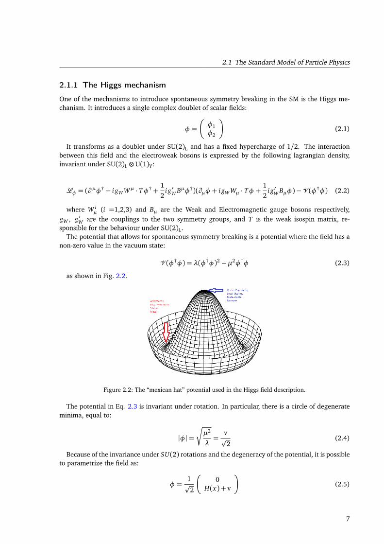
V (φ†φ) = λ(φ†φ)2−µ2φ†φ (2.3)
as shown in Fig. 2.2.
Figure 2.2: The “mexican hat” potential used in the Higgs field description.
The potential in Eq. 2.3 is invariant under rotation. In particular, there is a circle of degenerateminima, equal to:
|φ|=
r
µ2
λ=
vp
2(2.4)
Because of the invariance under SU(2) rotations and the degeneracy of the potential, it is possibleto parametrize the field as:
φ =1p
2
0H(x) + v
(2.5)
7
Chapter 2 Theory predictions for physics at the LHC
where v is the expectation value at the minimum and H(x) is a real function chosen for theparametrization of the field along the unbroken direction (i.e. the radial direction in Fig. 2.2).
In this parametrization, Eq. 2.2 shows quadratic terms that provide mass terms for the bosons:
Lbosons =v2(g2
W+ g′W2)
8ZµZµ+
v2g2W
4W−µ W+µ (2.6)
while no mass term exists for the Aµ field: the photon corresponds to a gauge transformationthat leaves φ invariant. The masses for the charged and neutral bosons are slightly different, asconfirmed in experiments, because the mass term for Zµ includes also the U(1) coupling constant.The other quadratic terms in the lagrangian provide mass terms and self coupling terms for theHiggs:
LHiggs =−µ2H2−λvH3−λH4
4=−
1
2mHH2−
r
λ
2mHH3−
λH4
4(2.7)
In the case of fermions, the Higgs field permits to introduce a Yukawa interaction of the formg f ψ fψ fφ, which will result in a mass term of the form m f =
vg f
2(as for the W± boson in Eq. 2.6).
The values of the Yukawa couplings are determined from the masses measured in experiments, anddon’t fulfill a fundamental requirement.
The terms of the lagrangian density containing the H(x) function from Eq. 2.5 are the interactionterms between the Higgs boson and the other particles. The coupling of the Higgs to the SMfermions can thus be written as:
gHiggs =
p2m f
v=
m f gW
2p
2mW(2.8)
2.2 QCD at high energy colliders
The LHC is a proton-proton collider. QCD effects will be dominant and need to be understoodfor a reliable physics analysis. For this reason, part of this thesis investigated the features of twoimportant QCD processes: di-jet production and the production of jets in association with a Zboson. These two processes also highlight fundamental properties of QCD, as it will be explainedin the next sections.
One fundamental property of QCD is that its coupling constant runs with energy, in a way suchthat it is relatively low at high energies and high at low energies. Because of this behaviour, quarkstend to form bound states very quickly, and are not observed as free particles in (low-energy)nature. Only baryons or mesons, i.e. color-neutral hadrons, are observed. However, the highenergy interactions observed in the LHC can be considered as interactions between the protonsconstituents, because at those high energy the physics is sensitive to the proton structure. Proton-proton collisions are thus divided into two main steps:
1. the hard interaction is calculated (using perturbation theory) considering only the elementarypartons, quarks or gluons, in the calculation of the matrix element
2. the result is then averaged over the composition of the proton, and taking into account higherorder effects.
8
2.2 QCD at high energy colliders
This separation is used extensively in QCD predictions: in the next sections, I will review itsmeaning and how it is implemented in particle physics studies.
2.2.1 The parton model of QCD
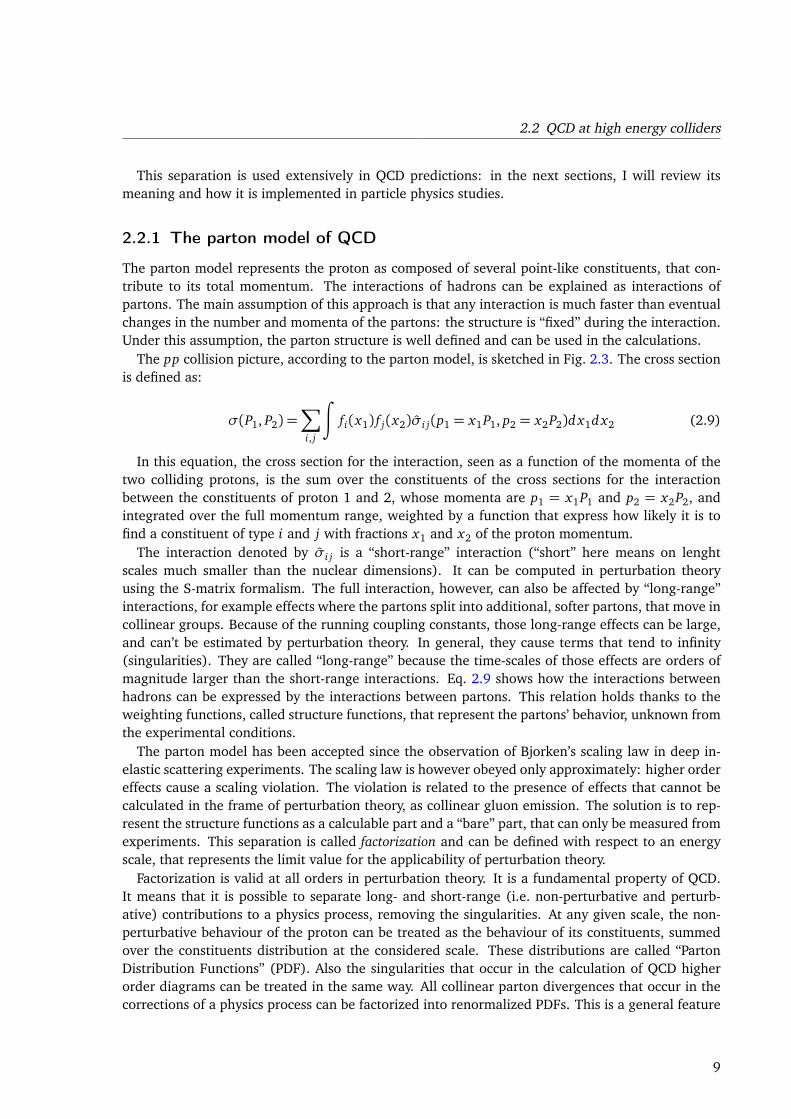
The parton model represents the proton as composed of several point-like constituents, that con-tribute to its total momentum. The interactions of hadrons can be explained as interactions ofpartons. The main assumption of this approach is that any interaction is much faster than eventualchanges in the number and momenta of the partons: the structure is “fixed” during the interaction.Under this assumption, the parton structure is well defined and can be used in the calculations.
The pp collision picture, according to the parton model, is sketched in Fig. 2.3. The cross sectionis defined as:
σ(P1, P2) =∑
i, j
∫
fi(x1) f j(x2)σi j(p1 = x1P1, p2 = x2P2)d x1d x2 (2.9)
In this equation, the cross section for the interaction, seen as a function of the momenta of thetwo colliding protons, is the sum over the constituents of the cross sections for the interactionbetween the constituents of proton 1 and 2, whose momenta are p1 = x1P1 and p2 = x2P2, andintegrated over the full momentum range, weighted by a function that express how likely it is tofind a constituent of type i and j with fractions x1 and x2 of the proton momentum.
The interaction denoted by σi j is a “short-range” interaction (“short” here means on lenghtscales much smaller than the nuclear dimensions). It can be computed in perturbation theoryusing the S-matrix formalism. The full interaction, however, can also be affected by “long-range”interactions, for example effects where the partons split into additional, softer partons, that move incollinear groups. Because of the running coupling constants, those long-range effects can be large,and can’t be estimated by perturbation theory. In general, they cause terms that tend to infinity(singularities). They are called “long-range” because the time-scales of those effects are orders ofmagnitude larger than the short-range interactions. Eq. 2.9 shows how the interactions betweenhadrons can be expressed by the interactions between partons. This relation holds thanks to theweighting functions, called structure functions, that represent the partons’ behavior, unknown fromthe experimental conditions.
The parton model has been accepted since the observation of Bjorken’s scaling law in deep in-elastic scattering experiments. The scaling law is however obeyed only approximately: higher ordereffects cause a scaling violation. The violation is related to the presence of effects that cannot becalculated in the frame of perturbation theory, as collinear gluon emission. The solution is to rep-resent the structure functions as a calculable part and a “bare” part, that can only be measured fromexperiments. This separation is called factorization and can be defined with respect to an energyscale, that represents the limit value for the applicability of perturbation theory.
Factorization is valid at all orders in perturbation theory. It is a fundamental property of QCD.It means that it is possible to separate long- and short-range (i.e. non-perturbative and perturb-ative) contributions to a physics process, removing the singularities. At any given scale, the non-perturbative behaviour of the proton can be treated as the behaviour of its constituents, summedover the constituents distribution at the considered scale. These distributions are called “PartonDistribution Functions” (PDF). Also the singularities that occur in the calculation of QCD higherorder diagrams can be treated in the same way. All collinear parton divergences that occur in thecorrections of a physics process can be factorized into renormalized PDFs. This is a general feature
9
Chapter 2 Theory predictions for physics at the LHC
f1(x1)
f2(x2)
P1
P2
x1P1
x2P2
σ1,2
spectator quarks
spectator quarks
final
stateparticles
Figure 2.3: Parton model description of a hard scattering event.
of inclusive hard scattering processes in hadron-hadron collisions.PDFs have been directly measured from fits to Deep-Inelastic-Scattering data. They show the
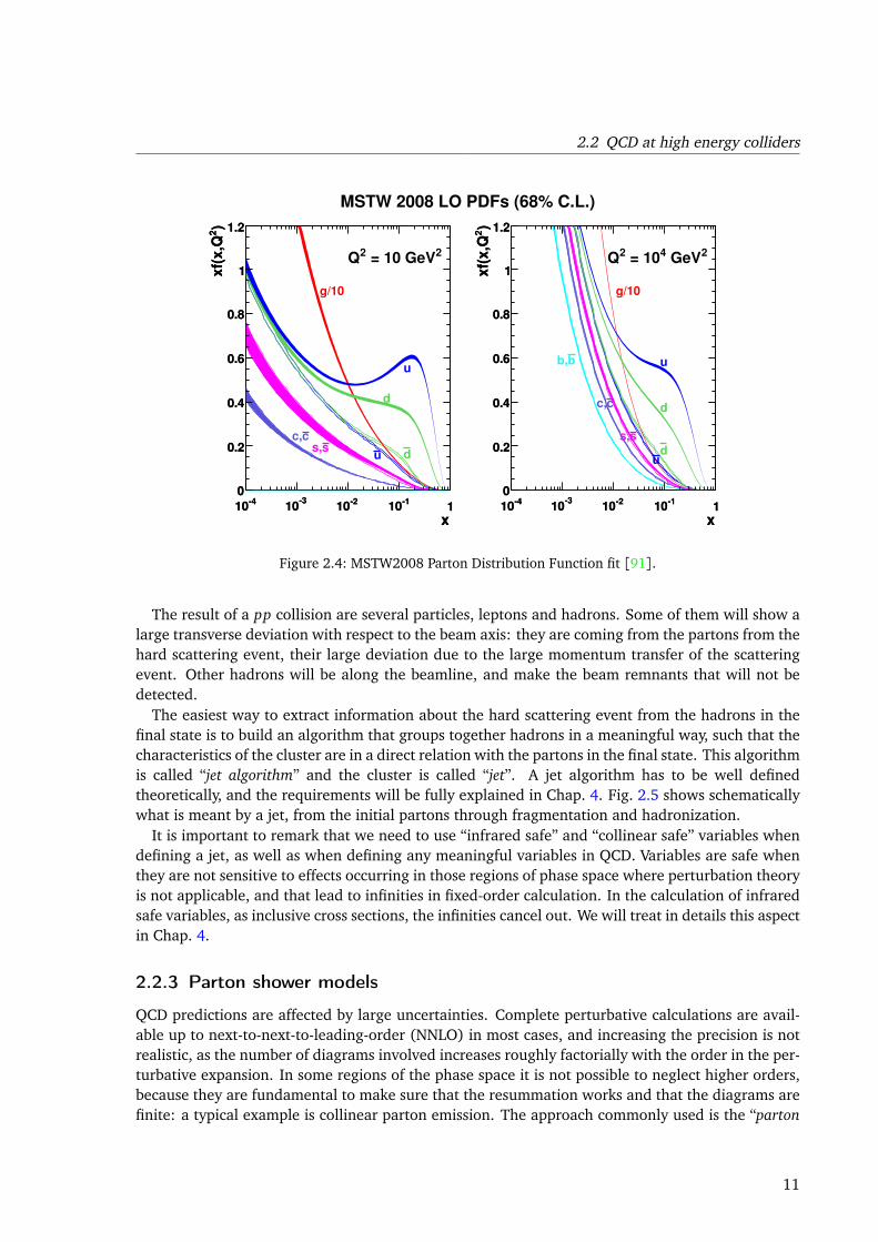
distribution of partons as a function of the momentum. In Fig. 2.4, one of the latest results isreported.
2.2.2 QCD properties and jets
Partons don’t exist as free particles in nature, but only inside colourless bound states. This propertyof “colour confinement” is one of the fundamental characteristics of QCD. The other main charac-teristic to bear in mind is the “asymptotic freedom”, i.e. the fact that the coupling constant of QCDruns with energy, such that it is very small at high energies (and low distances) and increases atlower energies.
These two properties of QCD will obviously affect the partons that take part to an interaction,and will determine the final state observed in the detector:
• because of asymptotic freedom, the collision between two partons can be divided into a short-and long-range contribution. Asymptotic freedom is the physical reason behind factorization.
• the hard scattering is a short-range event, and can be treated with perturbative QCD.
• long-range effects are represented in the process of fragmentation of the partons. Additionalpartons will be produced. The treatment of these long-range contributions is analogous tothe treatment of the initial state via PDFs.
• further decrease of the energy will cause the effects of confinement to become important.In this process, the quarks and gluons will combine into colourless hadrons (hadronization).Perturbation theory is not able to describe it; phenomenological models are used to makepredictions for the final state as it could be observed in a detector.
10
2.2 QCD at high energy colliders
x
-410
-310
-210
-110 1
)2
xf(
x,Q
0
0.2
0.4
0.6
0.8
1
1.2
g/10
d
d
u
uss,
cc,
2 = 10 GeV2Q
x
-410
-310
-210
-110 1
)2
xf(
x,Q
0
0.2
0.4
0.6
0.8
1
1.2
x
-410
-310
-210
-110 1
)2
xf(
x,Q
0
0.2
0.4
0.6
0.8
1
1.2
g/10
d
d
u
u
ss,
cc,
bb,
2 GeV4 = 102Q
x
-410
-310
-210
-110 1
)2
xf(
x,Q
0
0.2
0.4
0.6
0.8
1
1.2
MSTW 2008 LO PDFs (68% C.L.)
Figure 2.4: MSTW2008 Parton Distribution Function fit [91].
The result of a pp collision are several particles, leptons and hadrons. Some of them will show alarge transverse deviation with respect to the beam axis: they are coming from the partons from thehard scattering event, their large deviation due to the large momentum transfer of the scatteringevent. Other hadrons will be along the beamline, and make the beam remnants that will not bedetected.
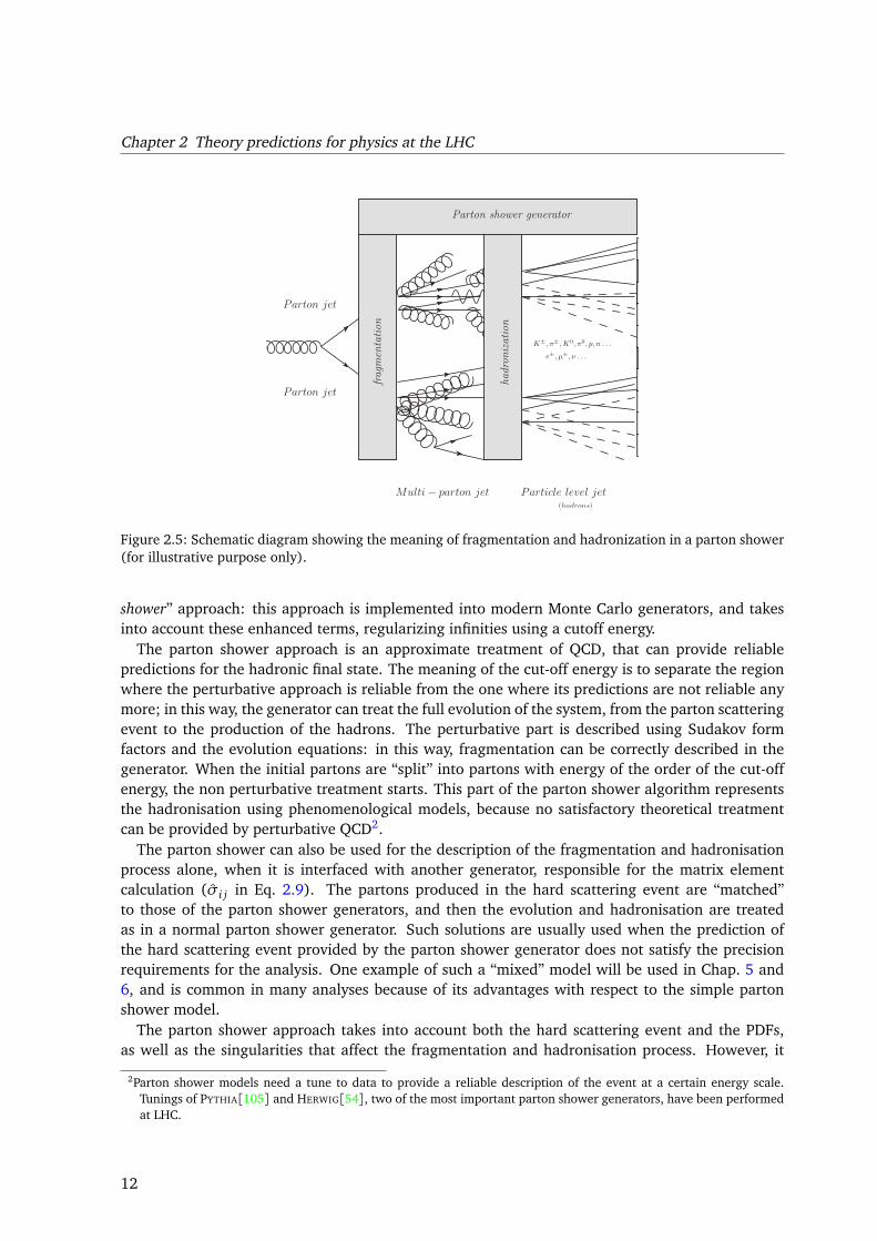
The easiest way to extract information about the hard scattering event from the hadrons in thefinal state is to build an algorithm that groups together hadrons in a meaningful way, such that thecharacteristics of the cluster are in a direct relation with the partons in the final state. This algorithmis called “jet algorithm” and the cluster is called “jet”. A jet algorithm has to be well definedtheoretically, and the requirements will be fully explained in Chap. 4. Fig. 2.5 shows schematicallywhat is meant by a jet, from the initial partons through fragmentation and hadronization.
It is important to remark that we need to use “infrared safe” and “collinear safe” variables whendefining a jet, as well as when defining any meaningful variables in QCD. Variables are safe whenthey are not sensitive to effects occurring in those regions of phase space where perturbation theoryis not applicable, and that lead to infinities in fixed-order calculation. In the calculation of infraredsafe variables, as inclusive cross sections, the infinities cancel out. We will treat in details this aspectin Chap. 4.
2.2.3 Parton shower models
QCD predictions are affected by large uncertainties. Complete perturbative calculations are avail-able up to next-to-next-to-leading-order (NNLO) in most cases, and increasing the precision is notrealistic, as the number of diagrams involved increases roughly factorially with the order in the per-turbative expansion. In some regions of the phase space it is not possible to neglect higher orders,because they are fundamental to make sure that the resummation works and that the diagrams arefinite: a typical example is collinear parton emission. The approach commonly used is the “parton
11
Chapter 2 Theory predictions for physics at the LHC
Parton jet
Parton jet
Multi− parton jet Particle level jet Calorimeter jet(hadrons) (detector level)
K±, π±,K0, π0, p, n . . .
e±, µ±, ν . . .
Parton shower generator
fragm
entation
hadronization
Figure 2.5: Schematic diagram showing the meaning of fragmentation and hadronization in a parton shower(for illustrative purpose only).
shower” approach: this approach is implemented into modern Monte Carlo generators, and takesinto account these enhanced terms, regularizing infinities using a cutoff energy.
The parton shower approach is an approximate treatment of QCD, that can provide reliablepredictions for the hadronic final state. The meaning of the cut-off energy is to separate the regionwhere the perturbative approach is reliable from the one where its predictions are not reliable anymore; in this way, the generator can treat the full evolution of the system, from the parton scatteringevent to the production of the hadrons. The perturbative part is described using Sudakov formfactors and the evolution equations: in this way, fragmentation can be correctly described in thegenerator. When the initial partons are “split” into partons with energy of the order of the cut-offenergy, the non perturbative treatment starts. This part of the parton shower algorithm representsthe hadronisation using phenomenological models, because no satisfactory theoretical treatmentcan be provided by perturbative QCD2.
The parton shower can also be used for the description of the fragmentation and hadronisationprocess alone, when it is interfaced with another generator, responsible for the matrix elementcalculation (σi j in Eq. 2.9). The partons produced in the hard scattering event are “matched”to those of the parton shower generators, and then the evolution and hadronisation are treatedas in a normal parton shower generator. Such solutions are usually used when the prediction ofthe hard scattering event provided by the parton shower generator does not satisfy the precisionrequirements for the analysis. One example of such a “mixed” model will be used in Chap. 5 and6, and is common in many analyses because of its advantages with respect to the simple partonshower model.
The parton shower approach takes into account both the hard scattering event and the PDFs,as well as the singularities that affect the fragmentation and hadronisation process. However, it
2Parton shower models need a tune to data to provide a reliable description of the event at a certain energy scale.Tunings of PYTHIA[105] and HERWIG[54], two of the most important parton shower generators, have been performedat LHC.
12
2.3 Z boson production in association with jets
might be still limited in treating the non-singular part of the cross section. Higher order correctionsin QCD are not small, but as said earlier often require too complex calculations to be estimated.Those effects may impact the value of the total cross section in a visible way. A common way totake into account those corrections is to define a “K-factor”, i.e. a correction factor that corrects thecross section calculated with the Monte Carlo generator at a finite order to the value calculatedat a higher order in the perturbative series. The K-factor can then be applied as a normalizationcorrection to the predicted number of events.
Parton shower generators are widely used in all HEP experiments. In ATLAS, the generator PYTH-IA[105] has been considered as a Monte Carlo reference for the jet studies performed in 2010. Inthe thesis (see Chap. 5) I have investigated the precision of the jet modelling provided by PYTHIA
comparing data and Monte Carlo events in an in-situ analysis, i.e. an analysis whose quantitiesdon’t need any Monte Carlo prediction or assumption to be derived. Also other parton generators(e.g. HERWIG[54]) have been compared to data in this analysis.
2.3 Z boson production in association with jets
With respect to QCD studies performed with jets, as inclusive jet cross section measurements, mea-surements involving vector bosons can provide a cleaner final state, that permits a better under-standing of the higher order QCD effects. Those are of fundamental importance in vector bosonproduction, as they are responsible for the production of vector bosons with a high transversemomentum.
q
q
Z/γ∗ ℓ
ℓ
(a) Feynman diagram for Drell-Yan process.
Z/γ∗
gluonjet
(b) Feynman diagram for production with a gluon jet inthe final state.
Z/γ∗
quarkjet
(c) Feynman diagram for production with a quark jet inthe final state.
q
q
Z/γ∗ ℓ
ℓ
(d) Feynman diagram for QCD loop correction in Drell-Yanprocess
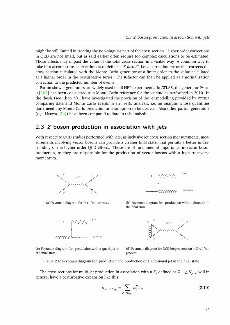
Figure 2.6: Feynman diagram for production and production of 1 additional jet in the final state.
The cross sections for multi-jet production in association with a Z , defined as Z+ ≥ Njets, will ingeneral have a perturbative expansion like this:
σZ+≥Njets=∑
N≥Njets
αNS aN (2.10)
13
Chapter 2 Theory predictions for physics at the LHC
It is clear to see that the cross section for the different jet multiplicity is expected to scale as afunction of α
Njets
S , the strong coupling constant at the power of the jet multiplicity considered. Termswith N > Njets are higher order QCD corrections.
When considering these corrections, the diagrams present infrared divergences. Fig. 2.6 showsthe relevant diagrams at order αS. Divergences involve either virtual gluon corrections graphs, orreal gluon corrections (emission of real gluons from one leg), or also quark gluon scattering process,where the Z is radiated off the scattered quark. The factorization theorem, however, guaranteesthat for these corrections the cancellation occurs, at each perturbative order. While the proof offactorization at all orders is still discussed by some authors, the possibility to measure the crosssections at different orders (i.e. for different jet multiplicity) and compare it with the predictionswould provide an indirect confirmation. Also, higher order corrections in QCD might be relativelylarge, and have a large impact on the precision of the prediction for this process.
The measurement of the Z cross section in association with jets, and its comparison with severalgenerator predictions, has been performed with 35 pb−1 and is reported in Chap. 6. To study theprocess with high precision, the analysis has focussed on the di-electron and di-muon final state.The di-tau final state presents higher uncertainties related to the reconstruction of the tau leptons.In particular, I have focussed on the di-muon final state: the probability of mis-reconstruct a muonas a jet or vice-versa are very low and, for this reason, it is very useful to study the hadronic part ofthe final state.
Several Monte Carlo predictions have been compared with the measurements, in order to es-timate how well commonly used generators can model this process. It is important to note thatthe most important generators used for these kind of processes (ALPGEN[90] and SHERPA[66]) aretree-level matrix-element generators: they compute only the first term of the perturbative series(α
Njets
S aNjetsfrom Eq. 2.10) for final states Z+≥ Njets. Up to Njets ≥ 5 has been considered. An agree-
ment or disagreement with the data could shed light on both the tree-level calculation, as wellas on the missing corrections. The measurement has also been compared with a NLO generator(BLACKHAT[41]).
Provided that the jet definition is infrared safe, the differential cross section as a function of thejet properties can provide important informations when compared with the theory. In this case,factorization ensures that the long-range effects show up only in collinear and infrared divergenceswhich cancel because of unitarity of the time evolution operator of the partons that originate thejet. Also in this case, the accuracy of tree-level generators has been studied with respect to themeasurement and to NLO calculations. Because jet production in Z → `` + jets events, as shownin Eq. 2.10, depends strongly on the order considered in the prediction, the phenomenologicalmodels used in parton shower generators might provide an inaccurate description of the process:the analysis confirmed this hypothesis.
2.4 Higgs boson production at LHC
The work presented in the last part of this thesis is part of the general ATLAS effort for the Higgsdiscovery. In 2011, the integrated luminosity was not high enough to ensure the discovery of theHiggs, and the results have been used to exclude a large part of the mass range. The results shownin Chap. 7 were also included in that combination.
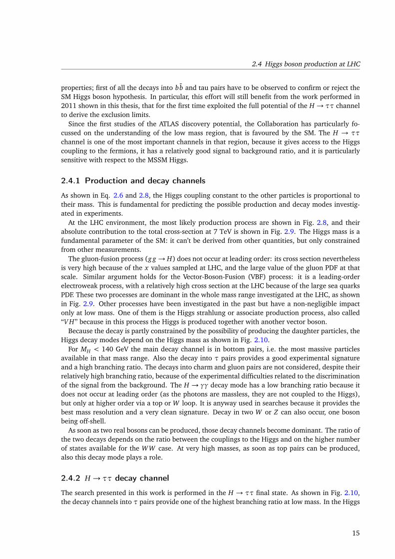
The preliminary results on the combination of 2011 and 2012 data show a 5σ excess at a massvalue of 126.5 GeV, shown in Fig. 2.7. The ATLAS results are consistent with the analogous resultsfrom CMS. The discovery of this new particle will be followed by additional studies targeting its
14
2.4 Higgs boson production at LHC
properties; first of all the decays into bb and tau pairs have to be observed to confirm or reject theSM Higgs boson hypothesis. In particular, this effort will still benefit from the work performed in2011 shown in this thesis, that for the first time exploited the full potential of the H → ττ channelto derive the exclusion limits.
Since the first studies of the ATLAS discovery potential, the Collaboration has particularly fo-cussed on the understanding of the low mass region, that is favoured by the SM. The H → ττ
channel is one of the most important channels in that region, because it gives access to the Higgscoupling to the fermions, it has a relatively good signal to background ratio, and it is particularlysensitive with respect to the MSSM Higgs.
2.4.1 Production and decay channels
As shown in Eq. 2.6 and 2.8, the Higgs coupling constant to the other particles is proportional totheir mass. This is fundamental for predicting the possible production and decay modes investig-ated in experiments.
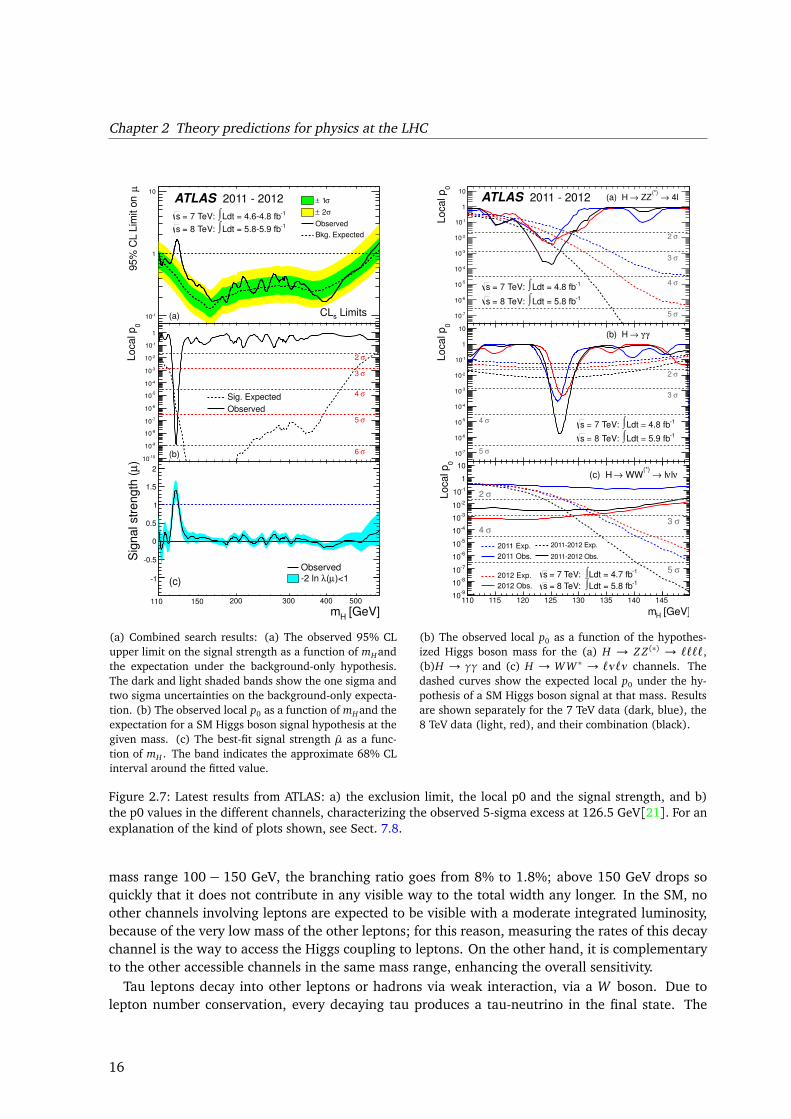
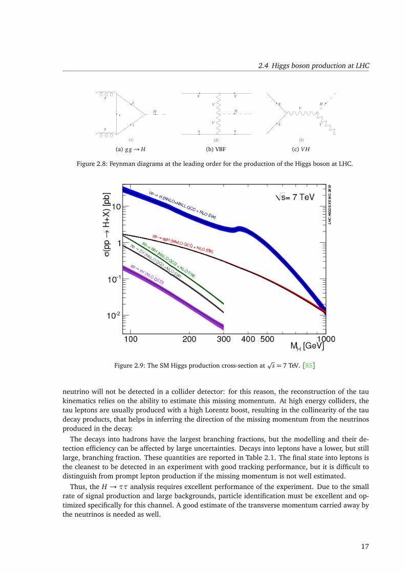
At the LHC environment, the most likely production process are shown in Fig. 2.8, and theirabsolute contribution to the total cross-section at 7 TeV is shown in Fig. 2.9. The Higgs mass is afundamental parameter of the SM: it can’t be derived from other quantities, but only constrainedfrom other measurements.
The gluon-fusion process (g g → H) does not occur at leading order: its cross section neverthelessis very high because of the x values sampled at LHC, and the large value of the gluon PDF at thatscale. Similar argument holds for the Vector-Boson-Fusion (VBF) process: it is a leading-orderelectroweak process, with a relatively high cross section at the LHC because of the large sea quarksPDF. These two processes are dominant in the whole mass range investigated at the LHC, as shownin Fig. 2.9. Other processes have been investigated in the past but have a non-negligible impactonly at low mass. One of them is the Higgs strahlung or associate production process, also called“V H” because in this process the Higgs is produced together with another vector boson.
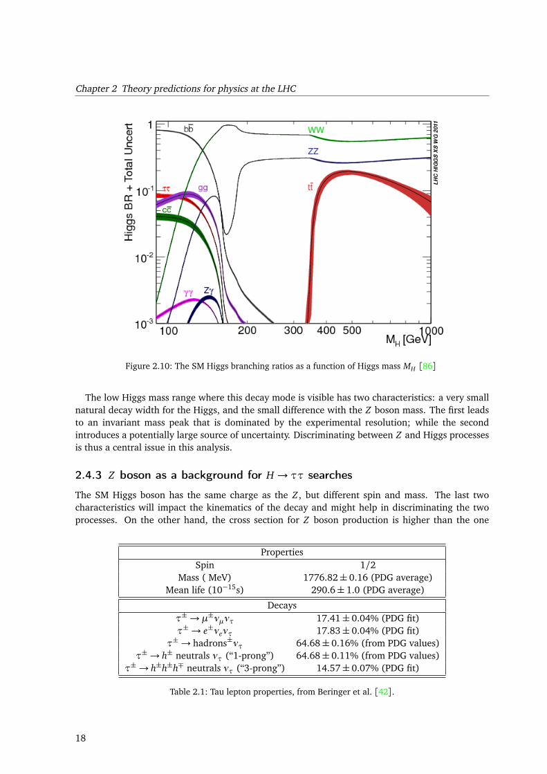
Because the decay is partly constrained by the possibility of producing the daughter particles, theHiggs decay modes depend on the Higgs mass as shown in Fig. 2.10.
For MH < 140 GeV the main decay channel is in bottom pairs, i.e. the most massive particlesavailable in that mass range. Also the decay into τ pairs provides a good experimental signatureand a high branching ratio. The decays into charm and gluon pairs are not considered, despite theirrelatively high branching ratio, because of the experimental difficulties related to the discriminationof the signal from the background. The H → γγ decay mode has a low branching ratio because itdoes not occur at leading order (as the photons are massless, they are not coupled to the Higgs),but only at higher order via a top or W loop. It is anyway used in searches because it provides thebest mass resolution and a very clean signature. Decay in two W or Z can also occur, one bosonbeing off-shell.
As soon as two real bosons can be produced, those decay channels become dominant. The ratio ofthe two decays depends on the ratio between the couplings to the Higgs and on the higher numberof states available for the WW case. At very high masses, as soon as top pairs can be produced,also this decay mode plays a role.
2.4.2 H → ττ decay channel
The search presented in this work is performed in the H → ττ final state. As shown in Fig. 2.10,the decay channels into τ pairs provide one of the highest branching ratio at low mass. In the Higgs
15
Chapter 2 Theory predictions for physics at the LHC
200 300 400 500
µ95%
CL L
imit o
n
110
1
10
σ 1±
σ 2±
Observed
Bkg. Expected
ATLAS 2011 20121Ldt = 4.64.8 fb∫ = 7 TeV: s 1Ldt = 5.85.9 fb∫ = 8 TeV: s
LimitssCL(a)
0Local p
1010
910
810
710
610
510
410
310
210
110
1
Sig. Expected
Observed
(b)
σ2
σ3
σ4
σ5
σ6
[GeV]H
m200 300 400 500
)µ
Sig
nal str
ength
(
1
0.5
0
0.5
1
1.5
2
Observed)<1µ(λ2 ln (c)
110 150
(a) Combined search results: (a) The observed 95% CLupper limit on the signal strength as a function of mHandthe expectation under the background-only hypothesis.The dark and light shaded bands show the one sigma andtwo sigma uncertainties on the background-only expecta-tion. (b) The observed local p0 as a function of mHand theexpectation for a SM Higgs boson signal hypothesis at thegiven mass. (c) The best-fit signal strength µ as a func-tion of mH . The band indicates the approximate 68% CLinterval around the fitted value.
110 115 120 125 130 135 140 145 150
0Local p
710
610
510
410
310
210
110
1
10
ATLAS 2011 2012 4l→ (*)
ZZ→(a) H
σ2
σ3
σ4
σ5
1Ldt = 4.8 fb∫ = 7 TeV: s 1Ldt = 5.8 fb∫ = 8 TeV: s
110 115 120 125 130 135 140 145 150
0Local p
710
610
510
410
310
210
110
1
10γγ →(b) H
σ2
σ3
σ4
σ5
1Ldt = 4.8 fb∫ = 7 TeV: s 1Ldt = 5.9 fb∫ = 8 TeV: s
[GeV]Hm110 115 120 125 130 135 140 145
0Local p
910
810
710
610
510
410
310
210
110
1
10
νlν l→ (*)
WW→(c) H
σ2
σ3 σ4
σ5
2011 Exp.
2011 Obs.
2012 Exp.
2012 Obs.
20112012 Exp.
20112012 Obs.
1Ldt = 4.7 fb∫ = 7 TeV: s 1Ldt = 5.8 fb∫ = 8 TeV: s
(b) The observed local p0 as a function of the hypothes-ized Higgs boson mass for the (a) H → Z Z (∗) → ````,(b)H → γγ and (c) H → WW ∗ → `ν`ν channels. Thedashed curves show the expected local p0 under the hy-pothesis of a SM Higgs boson signal at that mass. Resultsare shown separately for the 7 TeV data (dark, blue), the8 TeV data (light, red), and their combination (black).
Figure 2.7: Latest results from ATLAS: a) the exclusion limit, the local p0 and the signal strength, and b)the p0 values in the different channels, characterizing the observed 5-sigma excess at 126.5 GeV[21]. For anexplanation of the kind of plots shown, see Sect. 7.8.
mass range 100− 150 GeV, the branching ratio goes from 8% to 1.8%; above 150 GeV drops soquickly that it does not contribute in any visible way to the total width any longer. In the SM, noother channels involving leptons are expected to be visible with a moderate integrated luminosity,because of the very low mass of the other leptons; for this reason, measuring the rates of this decaychannel is the way to access the Higgs coupling to leptons. On the other hand, it is complementaryto the other accessible channels in the same mass range, enhancing the overall sensitivity.
Tau leptons decay into other leptons or hadrons via weak interaction, via a W boson. Due tolepton number conservation, every decaying tau produces a tau-neutrino in the final state. The
16
2.4 Higgs boson production at LHC
gt
g
H
t
(1)
t
(a) g g → H
q
H
q
q
(2)
q
V
V
(b) VBF
V
q
H
V
q
(3)
(c) V H
Figure 2.8: Feynman diagrams at the leading order for the production of the Higgs boson at LHC.
Figure 2.9: The SM Higgs production cross-section atp
s = 7 TeV. [85]
neutrino will not be detected in a collider detector: for this reason, the reconstruction of the taukinematics relies on the ability to estimate this missing momentum. At high energy colliders, thetau leptons are usually produced with a high Lorentz boost, resulting in the collinearity of the taudecay products, that helps in inferring the direction of the missing momentum from the neutrinosproduced in the decay.
The decays into hadrons have the largest branching fractions, but the modelling and their de-tection efficiency can be affected by large uncertainties. Decays into leptons have a lower, but stilllarge, branching fraction. These quantities are reported in Table 2.1. The final state into leptons isthe cleanest to be detected in an experiment with good tracking performance, but it is difficult todistinguish from prompt lepton production if the missing momentum is not well estimated.
Thus, the H → ττ analysis requires excellent performance of the experiment. Due to the smallrate of signal production and large backgrounds, particle identification must be excellent and op-timized specifically for this channel. A good estimate of the transverse momentum carried away bythe neutrinos is needed as well.
17
Chapter 2 Theory predictions for physics at the LHC
Figure 2.10: The SM Higgs branching ratios as a function of Higgs mass MH [86]
The low Higgs mass range where this decay mode is visible has two characteristics: a very smallnatural decay width for the Higgs, and the small difference with the Z boson mass. The first leadsto an invariant mass peak that is dominated by the experimental resolution; while the secondintroduces a potentially large source of uncertainty. Discriminating between Z and Higgs processesis thus a central issue in this analysis.
2.4.3 Z boson as a background for H → ττ searches
The SM Higgs boson has the same charge as the Z , but different spin and mass. The last twocharacteristics will impact the kinematics of the decay and might help in discriminating the twoprocesses. On the other hand, the cross section for Z boson production is higher than the one
PropertiesSpin 1/2
Mass ( MeV) 1776.82± 0.16 (PDG average)Mean life (10−15s) 290.6± 1.0 (PDG average)
Decaysτ±→ µ±νµντ 17.41± 0.04% (PDG fit)τ±→ e±νeντ 17.83± 0.04% (PDG fit)
τ±→ hadrons±ντ 64.68± 0.16% (from PDG values)τ±→ h± neutrals ντ (“1-prong”) 64.68± 0.11% (from PDG values)
τ±→ h±h±h∓ neutrals ντ (“3-prong”) 14.57± 0.07% (PDG fit)
Table 2.1: Tau lepton properties, from Beringer et al. [42].
18
2.4 Higgs boson production at LHC
for Higgs production by four orders of magnitude. Because of the similarities between the twoprocesses, this process is one of the most important irreducible backgrounds for searches at lowmass considering a fermionic decay of the Higgs boson.
As the suppression of the Z background is not completely possible, it is of fundamental import-ance to carefully estimate it. To estimate the contribution of this process to the total yield of events,first we need a reliable value for the inclusive cross section, as well as the values for the differentialcross sections. The inclusive cross section is known up to a precision of few percent[16], but theprecision gets worse when the events are split according to the parton multiplicity. In the analysisreported in Chap. 6, several differential cross sections, used to highlight the difference between theHiggs signal and the background, have been carefully studied to check the agreement between theprediction and the data.
In the H → ττ→ ``+ 4ν channel, studied in Chap. 7, the main background is indeed Z bosonproduction, with all lepton flavours to be taken into account (τ considered only in case of a leptonicdecay). Even though the Z → `` + jets analysis shows a reasonable agreement between data andthe simulations, the strategy is to not use the simulation predictions blindly in the analysis, becausetheir uncertainties could impact strongly the analysis. An example is the possibility to distinguishbetween the Z → ττ background and a Higgs signal: experimental effects can affect significantlythe Emiss
T reconstruction, fundamental for the mass reconstruction and the separation between thetwo processes. A poorly modelled Emiss
T can have a large impact on the limit derived. For thisreason, the Z → ττ background is derived from the data, using the so-called “embedding method”(see Sect. 7.6.2). The Z → `` + jets background, more independent from Emiss
T modelling becauseno real Emiss
T is expected in the event, was instead estimated from simulations, and corrected usingdata-Monte Carlo comparisons performed in control (i.e. signal-free) regions.
2.4.4 Theoretical uncertainties on Higgs cross sections
The values predicted by the theory are affected by uncertainties. The uncertainties arise fromtwo sources: the missing higher-order corrections yield the “theoretical” uncertainties, while theexperimental errors on the SM input parameters, such as the quark masses or the strong couplingconstant, give rise to the “parametric” uncertainties.
Concerning the branching ratio, the full calculation of the uncertainty is reported in LHC HiggsCross Section Working Group et al. [86]. The relative importance of the theoretical and paramet-ric uncertainties depends on the channel, with decay channels into quarks and gluons being moreaffected, on average, by parametric uncertainties than the other channels. On average, the uncer-tainties are of the order of 5%.
For the production processes, the treatment is more complicated, because it needs to include thelimited knowledge of the PDFs. The production processes will be affected in a different way bythe PDFs, because of the differences in the initial state. The full calculation of the uncertainties onthe inclusive cross section is reported in LHC Higgs Cross Section Working Group et al. [85]. Theuncertainty shows almost no trend with the Higgs mass, and are of the order of 20% for g g → H,3% for VBF, and 4− 5% for VH.
When considering the differential distributions, other uncertainties arise. In the case of g g → H,the fact that the process is not a leading-order process, and the need for a high precision, suggestsan effective field theory approach. This is in general reasonable, mostly for low mH , but couldintroduce distortions in some of the distributions, most notably in case of large Higgs pT, wherethe process is sensitive to the bottom and top quark finite masses (not considered in an effectiveapproach). This distortion can be of O (10%) in these regions, while are within few percent in the
19
Chapter 2 Theory predictions for physics at the LHC
total cross section and in the rapidity distribution. The analyses fix this issue implementing a re-weighting of the finite-order predictions to the values predicted at a higher order of the calculation.
Other very useful exclusive approaches are those that separate events with additional partonsin the final state, from those with no additional partons. This is motivated by the backgroundcomposition of the Higgs signal, that is different in the two cases. The prediction is accurateenough for VBF and VH. The effective approach used in g g → H, instead, induces large logarithmsto appear when the g g → H cross-section calculation is split according to the number of partons inthe final state (they would cancel out only in the inclusive cross section). Those logarithms can’tbe resummed and their contribution must be evaluated for each case and then combined. Thefull treatment is reported in LHC Higgs Cross Section Working Group et al. [86]; the procedure toestimate those uncertainties reliably and the way it has been implemented in our analysis will besummarized in Sect. 7.2.
The last ingredient to take into account for a correct estimate of the theoretical uncertainty isthe additional approximations that are done in the generators commonly used for the predictionsat the detector level, and not only for the very precise calculations. For the experimental analysis,Monte Carlo generators that provide a finite-order calculation of the cross section are used. TheHiggs cross section working group has carefully studied the differential distributions for the Higgsin several generators and compared this with the next-to-next-to-leading-order (NNLO) prediction[86], to estimate the uncertainty of the generators. In general, the results obtained with thosegenerators have been reweighted to correct their output to the highest order level. This is particu-larly important for QCD effects, that are estimated via parton shower methods and provide a LOprecision. Those effects affect largely all production processes, and have been carefully investig-ated for two processes: g g → H (where partons in the final state can be created only from QCDradiation) and VBF (where two leading partons in the final state are expected at leading order).The prescription of the LHC Cross Section Working Group has been implemented in the analysis, aswill be explained in Sect. 7.3.
20
Chapter 3
The LHC and the ATLAS experiment
The Large Hadron Collider has been conceived as a global project. This effort has an importancebeyond the understanding of the missing pieces of particle physics, and inspects other issues ofmodern physics, for example the lack of a candidate for dark matter[69]. The project was approvedin 1991, as natural continuation of the LEP experiments.
3.1 The Large Hadron Collider
The Large Hadron Collider (LHC) is a two-ring-superconducting hadron accelerator and collider,installed in the existing 26.7 km tunnel that was constructed between 1984 and 1989 for the CERN
Figure 3.1: Representation of LHC.
21

Chapter 3 The LHC and the ATLAS experiment
LEP collider. The LEP tunnel has eight straight sections and eight arcs, and lies between 45 m and170 m below the surface, near Geneva, across the Swiss-French border.
The tunnel in the arcs has an internal diameter of 3.7 m, which makes it extremely difficult toinstall two completely separated proton rings. This hard limit on space led to the adoption of thetwin-bore magnet design1, shown in Fig. 3.2. The extremely high energy target led to the use ofsuperconducting magnets to reach the high currents needed. The LHC magnet system cools themagnets to a temperature below 2 K, using super-fluid helium, and could operate at fields above 8T.
Figure 3.2: LHC dipole section, schematic drawing.[2]
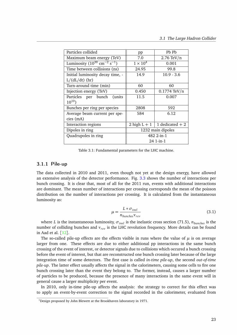
Table 3.1 lists the fundamental parameters for the LHC machine, both for the pp and the heavyion collisions.
Inside the LHC ring, bunches of up to 1011 protons collide, by design, every 25 ns (40 milliontimes every second). Such a high interaction rate is needed because of the small cross sectionsexpected for the process of interest. The inelastic pp cross section is 80 mb; thus the LHC isexpected, at design energy and bunch settings, to produce a total rate of 109 inelastic events persecond. This puts a serious experimental difficulty, because it implies that interesting hard collisionswill occur together with additional 23 inelastic events per bunch-crossing on average. This problemis called pile-up.
22
3.1 The Large Hadron Collider
Particles collided pp Pb PbMaximum beam energy (TeV) 7.0 2.76 TeV/nLuminosity (1030 cm−2 s−1) 1× 10⁴ 0.001Time between collisions (ns) 24.95 99.8Initial luminosity decay time, -L/(dL/dt) (hr)
14.9 10.9 - 3.6
Turn-around time (min) 60 60Injection energy (TeV) 0.450 0.1774 TeV/nParticles per bunch (units1010)
11.5 0.007
Bunches per ring per species 2808 592Average beam current per spe-cies (mA)
584 6.12
Interaction regions 2 high L + 1 1 dedicated + 2Dipoles in ring 1232 main dipolesQuadrupoles in ring 482 2-in-1
24 1-in-1
Table 3.1: Fundamental parameters for the LHC machine.
3.1.1 Pile-up
The data collected in 2010 and 2011, even though not yet at the design energy, have allowedan extensive analysis of the detector performance. Fig. 3.3 shows the number of interactions perbunch crossing. It is clear that, most of all for the 2011 run, events with additional interactionsare dominant. The mean number of interactions per crossing corresponds the mean of the poissondistribution on the number of interactions per crossing. It is calculated from the instantaneousluminosity as:
µ=L ∗σinel
nbunchesνrev(3.1)
where L is the instantaneous luminosity, σinel is the inelastic cross section (71.5), nbunches is thenumber of colliding bunches and νrev is the LHC revolution frequency. More details can be foundin Aad et al. [12].
The so-called pile-up effects are the effects visible in runs where the value of µ is on averagelarger from one. These effects are due to either additional pp interactions in the same bunchcrossing of the event of interest, or detector signals due to collisions which occured a bunch crossingbefore the event of interest, but that are reconstructed one bunch crossing later because of the largeintegration time of some detectors. The first case is called in-time pile-up, the second out-of-timepile-up. The latter effect usually affects the signal in the calorimeters, causing some cells to fire onebunch crossing later than the event they belong to. The former, instead, causes a larger numberof particles to be produced, because the presence of many interactions in the same event will ingeneral cause a larger multiplicity per event.
In 2010, only in-time pile-up affects the analysis: the strategy to correct for this effect wasto apply an event-by-event correction to the signal recorded in the calorimeter, evaluated from
1Design proposed by John Blewett at the Brookhaven laboratory in 1971.
23
Chapter 3 The LHC and the ATLAS experiment
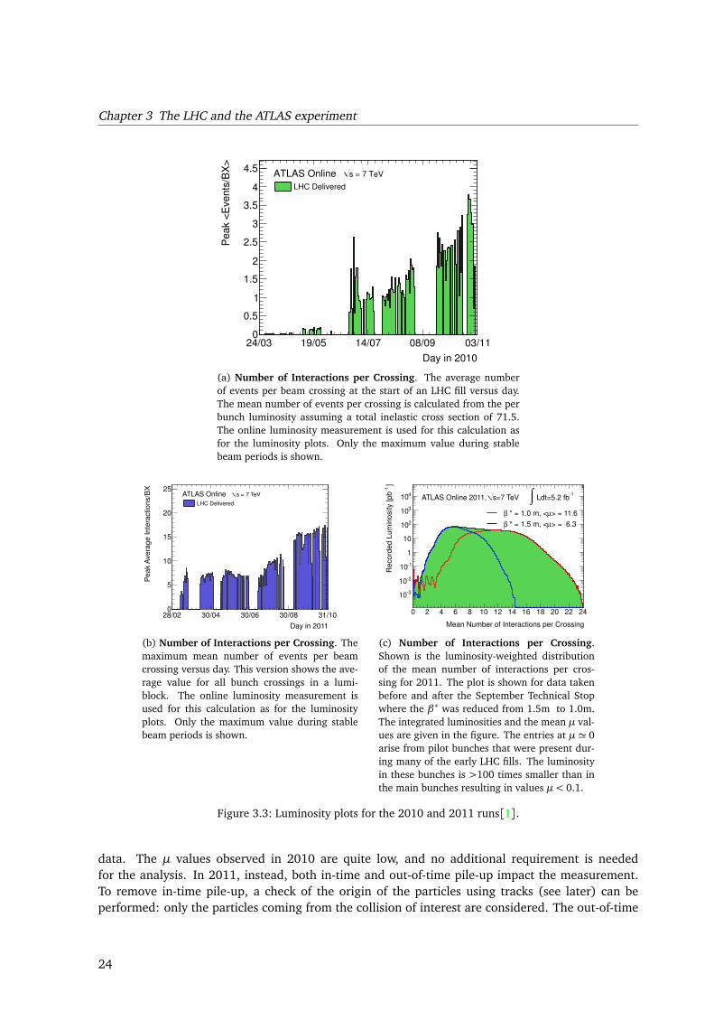
Day in 2010
24/03 19/05 14/07 08/09 03/11
Peak <
Events
/BX
>
0
0.5
1
1.5
2
2.5
3
3.5
4
4.5 = 7 TeVs ATLAS Online
LHC Delivered
(a) Number of Interactions per Crossing. The average numberof events per beam crossing at the start of an LHC fill versus day.The mean number of events per crossing is calculated from the perbunch luminosity assuming a total inelastic cross section of 71.5.The online luminosity measurement is used for this calculation asfor the luminosity plots. Only the maximum value during stablebeam periods is shown.
Day in 2011
28/02 30/04 30/06 30/08 31/10
Pe
ak A
ve
rag
e Inte
ractio
ns/B
X
0
5
10
15
20
25 = 7 TeVs ATLAS Online
LHC Delivered
(b) Number of Interactions per Crossing. Themaximum mean number of events per beamcrossing versus day. This version shows the ave-rage value for all bunch crossings in a lumi-block. The online luminosity measurement isused for this calculation as for the luminosityplots. Only the maximum value during stablebeam periods is shown.
Mean Number of Interactions per Crossing
0 2 4 6 8 10 12 14 16 18 20 22 24
]1
Record
ed L
um
inosity [pb
310
210
110
1
10
210
310
410 =7 TeVsATLAS Online 2011, 1
Ldt=5.2 fb∫> = 11.6µ * = 1.0 m, <β
> = 6.3µ * = 1.5 m, <β
(c) Number of Interactions per Crossing.Shown is the luminosity-weighted distributionof the mean number of interactions per cros-sing for 2011. The plot is shown for data takenbefore and after the September Technical Stopwhere the β∗ was reduced from 1.5m to 1.0m.The integrated luminosities and the mean µ val-ues are given in the figure. The entries at µ ' 0arise from pilot bunches that were present dur-ing many of the early LHC fills. The luminosityin these bunches is >100 times smaller than inthe main bunches resulting in values µ < 0.1.
Figure 3.3: Luminosity plots for the 2010 and 2011 runs[1].
data. The µ values observed in 2010 are quite low, and no additional requirement is neededfor the analysis. In 2011, instead, both in-time and out-of-time pile-up impact the measurement.To remove in-time pile-up, a check of the origin of the particles using tracks (see later) can beperformed: only the particles coming from the collision of interest are considered. The out-of-time
24
3.2 The ATLAS detector
pile-up effect on the reconstructed calorimeter energy was instead estimated as a function of thenumber of primary vertices in simulations, and cross-checked with data. Both corrections aim toremove any possible dependence of the measured quantities on the vertex multiplicity.
3.2 The ATLAS detector
The ATLAS detector started commissioning operations in autumn 2007 at the LHC Intersection Point1, and started taking stable beams data2 since beginning of 2010. The collaboration started in theearly 90s, as the joined effort of two previous concepts for a new detector at the LHC accelerator,when the LEP collider at CERN was still in operation. In 2004 a combined test beam for the firsttime took data with all the detector components (small prototypes or single modules) workingtogheter, using a pion beam accelerated by the PS facility. The data have been used for initialcommissioning and calibration of several parts of the detector; in particular, they have provided theinitial calibration for the calorimeters.
In 2004 the first parts of the detector were installed in the cavern, while the last part was insertedin 2007. Because of problems at the LHC facilities, however, beam operations started only in late2009.
For the main goals and a more complete description of the ATLAS experiment, we refer thereader to ATLAS: technical proposal for a general-purpose pp experiment at the Large Hadron Colliderat CERN [4] and Aad et al. [31].
3.2.1 Overall detector
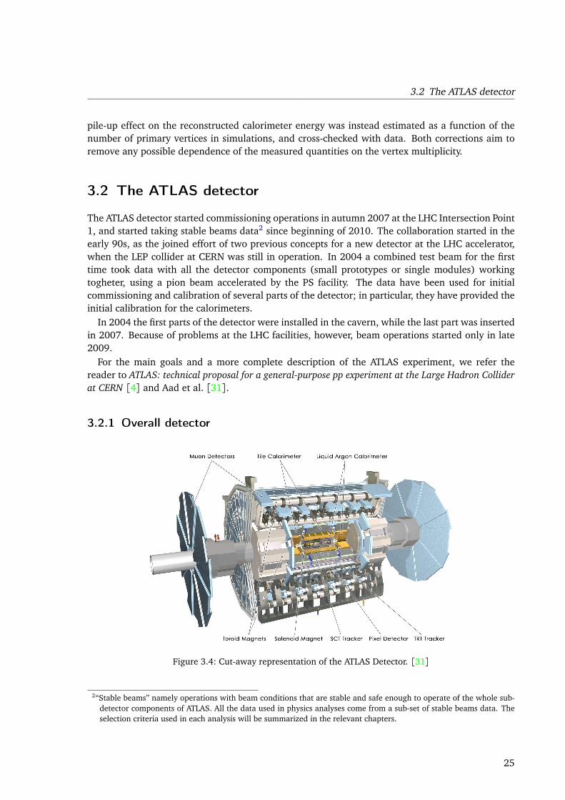
Figure 3.4: Cut-away representation of the ATLAS Detector. [31]
2“Stable beams” namely operations with beam conditions that are stable and safe enough to operate of the whole sub-detector components of ATLAS. All the data used in physics analyses come from a sub-set of stable beams data. Theselection criteria used in each analysis will be summarized in the relevant chapters.
25

Chapter 3 The LHC and the ATLAS experiment
The ATLAS detector is composed of several stratified subsystems, responsible for different mea-surements, that will provide the complete information needed for the physics analysis.
The principal requirements for LHC detectors are mainly due to the high energy and luminosity.Thus the detector has strict constraints on resolution, timing performance, geometry, and radiationhardness; they can be mainly summarised as:
• Fast and radiation-hard on-detector electronics. The high fluxes require a high detector gra-nularity.
• Large acceptance, almost all solid angle covered.
• Good charged particle momentum measurement and reconstruction efficiency, to be mea-sured with a very precise tracker. To observe secondary vertices with high precision, thevertex detector should be as close as possible to the interaction region.
• Good calorimetry performance to identify particles and measure their energies; by the meansof an electromagnetic calorimeter for electron and photon identification and measurements,and a hadronic calorimeter, to measure jets and missing transverse energy.
• Good muon identification and measurement - especially for high pT muons.
• Highly efficient trigger on low momentum objects, with sufficient background rejection, toachieve an acceptable trigger rate.
The ATLAS detector reaches 44 m in length along the beam axis, while its height is 25 m. It iscomposed of 6 different detector subsystems and 2 magnet subsystems.
3.2.2 Coordinate system and conventions
Conventionally the z direction is set along the beam axis, while x and y are in the transverseplane. Polar coordinates are often used in the transverse plane, with the R coordinate describingthe radial position from the beam axis, and the φ coordinate describing the azimuthal angle. Theconventional coordinate for angular position with respect to the beam axis is the pseudorapidity,defined as η=− ln tan(θ/2), where θ is the angle with the beam axis.
Due to the shape of the detector, the central region is also called the barrel, while the two sidesare called end-caps.
3.2.3 Inner Detector (Tracker)
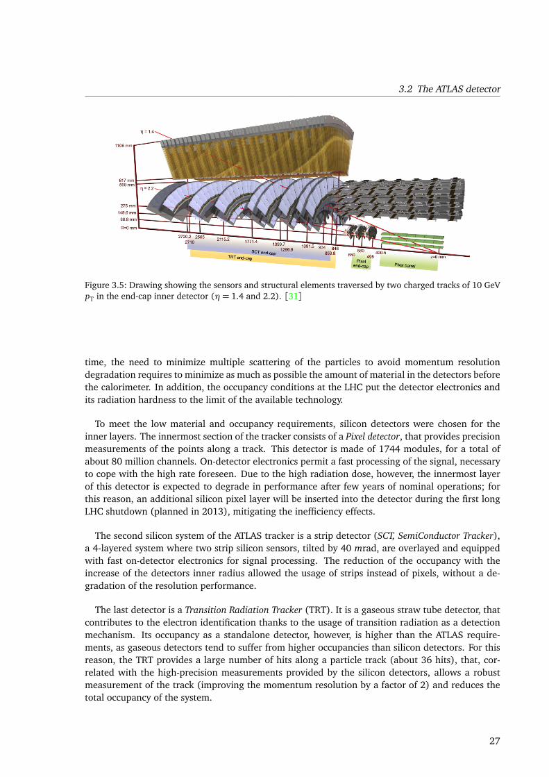
The Inner Detector is the innermost part of the detector, and provides tracking measurements andreconstruction of secondary vertices. It is immersed in a 2 T magnetic field provided by a super-conducting solenoid magnet, placed just outside the Inner Detector volume. It is sketched in Fig.3.5, where also the dimension of the detector and its coverage in η are highlighted. The maximumcoverage of the detector is |η|< 2.5.
The dimensions and characteristics of such a system are determined by space requirements: onone side, the inner radius must be larger than the beam pipe radius, on the other side, the outerradius must be smaller than the solenoid needed to curve charged particles in the innermost partof the detector. The solenoid dimensions are limited by the calorimeter requirements, that arephysics requirements related to the spatial resolution of electromagnetic showers. At the same
26
3.2 The ATLAS detector
Figure 3.5: Drawing showing the sensors and structural elements traversed by two charged tracks of 10 GeVpT in the end-cap inner detector (η= 1.4 and 2.2). [31]
time, the need to minimize multiple scattering of the particles to avoid momentum resolutiondegradation requires to minimize as much as possible the amount of material in the detectors beforethe calorimeter. In addition, the occupancy conditions at the LHC put the detector electronics andits radiation hardness to the limit of the available technology.
To meet the low material and occupancy requirements, silicon detectors were chosen for theinner layers. The innermost section of the tracker consists of a Pixel detector, that provides precisionmeasurements of the points along a track. This detector is made of 1744 modules, for a total ofabout 80 million channels. On-detector electronics permit a fast processing of the signal, necessaryto cope with the high rate foreseen. Due to the high radiation dose, however, the innermost layerof this detector is expected to degrade in performance after few years of nominal operations; forthis reason, an additional silicon pixel layer will be inserted into the detector during the first longLHC shutdown (planned in 2013), mitigating the inefficiency effects.
The second silicon system of the ATLAS tracker is a strip detector (SCT, SemiConductor Tracker),a 4-layered system where two strip silicon sensors, tilted by 40 mrad, are overlayed and equippedwith fast on-detector electronics for signal processing. The reduction of the occupancy with theincrease of the detectors inner radius allowed the usage of strips instead of pixels, without a de-gradation of the resolution performance.
The last detector is a Transition Radiation Tracker (TRT). It is a gaseous straw tube detector, thatcontributes to the electron identification thanks to the usage of transition radiation as a detectionmechanism. Its occupancy as a standalone detector, however, is higher than the ATLAS require-ments, as gaseous detectors tend to suffer from higher occupancies than silicon detectors. For thisreason, the TRT provides a large number of hits along a particle track (about 36 hits), that, cor-related with the high-precision measurements provided by the silicon detectors, allows a robustmeasurement of the track (improving the momentum resolution by a factor of 2) and reduces thetotal occupancy of the system.
27
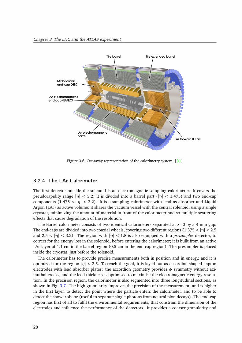
Chapter 3 The LHC and the ATLAS experiment
Figure 3.6: Cut-away representation of the calorimetry system. [31]
3.2.4 The LAr Calorimeter
The first detector outside the solenoid is an electromagnetic sampling calorimeter. It covers thepseudorapidity range |η| < 3.2; it is divided into a barrel part (|η| < 1.475) and two end-capcomponents (1.475 < |η| < 3.2). It is a sampling calorimeter with lead as absorber and LiquidArgon (LAr) as active volume; it shares the vacuum vessel with the central solenoid, using a singlecryostat, minimizing the amount of material in front of the calorimeter and so multiple scatteringeffects that cause degradation of the resolution.
The Barrel calorimeter consists of two identical calorimeters separated at z=0 by a 4 mm gap.The end-caps are divided into two coaxial wheels, covering two different regions (1.375< |η|< 2.5and 2.5 < |η| < 3.2). The region with |η| < 1.8 is also equipped with a presampler detector, tocorrect for the energy lost in the solenoid, before entering the calorimeter; it is built from an activeLAr layer of 1.1 cm in the barrel region (0.5 cm in the end-cap region). The presampler is placedinside the cryostat, just before the solenoid.
The calorimeter has to provide precise measurements both in position and in energy, and it isoptimized for the region |η| < 2.5. To reach the goal, it is layed out as accordion-shaped kaptonelectrodes with lead absorber plates: the accordion geometry provides φ symmetry without azi-muthal cracks, and the lead thickness is optimised to maximise the electromagnetic energy resolu-tion. In the precision region, the calorimeter is also segmented into three longitudinal sections, asshown in Fig. 3.7. The high granularity improves the precision of the measurement, and is higherin the first layer, to detect the point where the particle enters the calorimeter, and to be able todetect the shower shape (useful to separate single photons from neutral pion decays). The end-capregion has first of all to fulfil the environmental requirements, that constrain the dimension of theelectrodes and influence the performance of the detectors. It provides a coarser granularity and
28
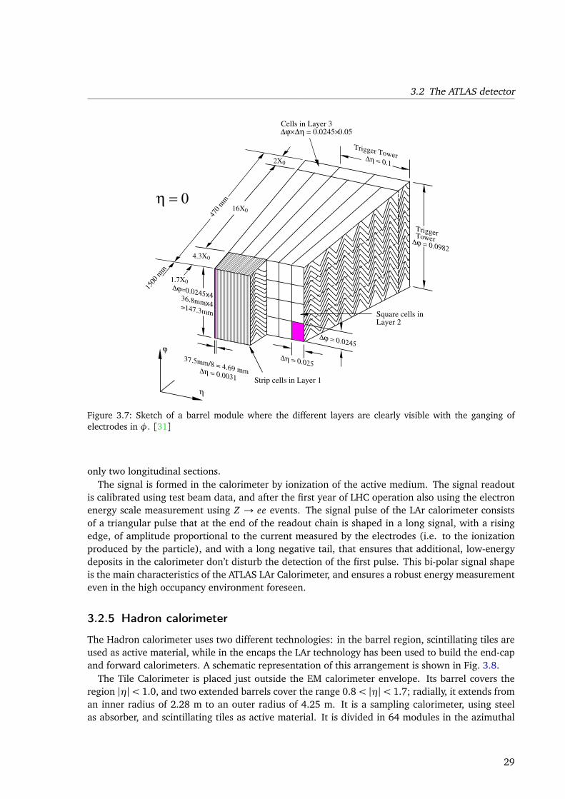
3.2 The ATLAS detector
∆ϕ = 0.0245
∆η = 0.02537.5mm/8 = 4.69 mm ∆η = 0.0031
∆ϕ=0.0245x4 36.8mmx4 =147.3mm
Trigger Tower
TriggerTower∆ϕ = 0.0982
∆η = 0.1
16X0
4.3X0
2X0
1500
mm
470 m
m
η
ϕ
η = 0
Strip cells in Layer 1
Square cells in Layer 2
1.7X0
Cells in Layer 3 ∆ϕ×∆η = 0.0245×0.05
Figure 3.7: Sketch of a barrel module where the different layers are clearly visible with the ganging ofelectrodes in φ. [31]
only two longitudinal sections.The signal is formed in the calorimeter by ionization of the active medium. The signal readout
is calibrated using test beam data, and after the first year of LHC operation also using the electronenergy scale measurement using Z → ee events. The signal pulse of the LAr calorimeter consistsof a triangular pulse that at the end of the readout chain is shaped in a long signal, with a risingedge, of amplitude proportional to the current measured by the electrodes (i.e. to the ionizationproduced by the particle), and with a long negative tail, that ensures that additional, low-energydeposits in the calorimeter don’t disturb the detection of the first pulse. This bi-polar signal shapeis the main characteristics of the ATLAS LAr Calorimeter, and ensures a robust energy measurementeven in the high occupancy environment foreseen.
3.2.5 Hadron calorimeter
The Hadron calorimeter uses two different technologies: in the barrel region, scintillating tiles areused as active material, while in the encaps the LAr technology has been used to build the end-capand forward calorimeters. A schematic representation of this arrangement is shown in Fig. 3.8.
The Tile Calorimeter is placed just outside the EM calorimeter envelope. Its barrel covers theregion |η|< 1.0, and two extended barrels cover the range 0.8< |η|< 1.7; radially, it extends froman inner radius of 2.28 m to an outer radius of 4.25 m. It is a sampling calorimeter, using steelas absorber, and scintillating tiles as active material. It is divided in 64 modules in the azimuthal
29
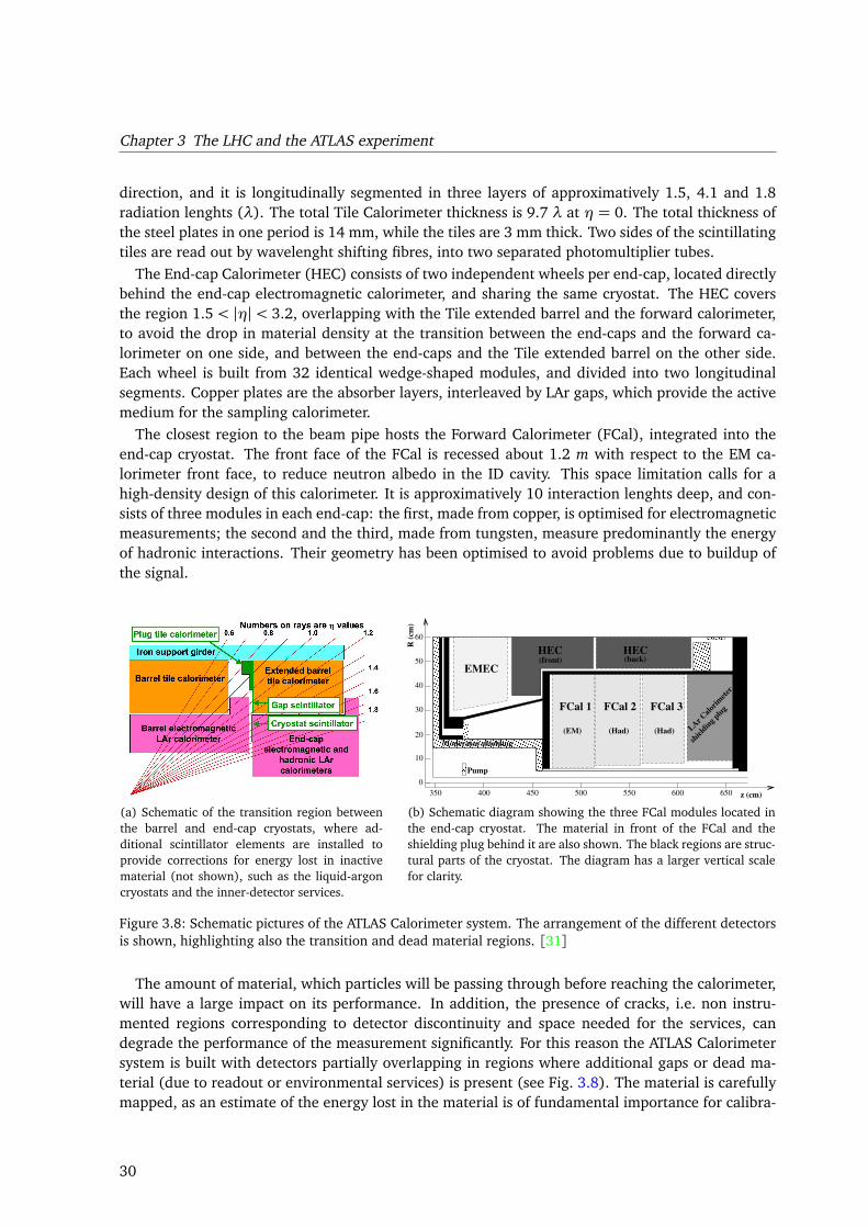
Chapter 3 The LHC and the ATLAS experiment
direction, and it is longitudinally segmented in three layers of approximatively 1.5, 4.1 and 1.8radiation lenghts (λ). The total Tile Calorimeter thickness is 9.7 λ at η = 0. The total thickness ofthe steel plates in one period is 14 mm, while the tiles are 3 mm thick. Two sides of the scintillatingtiles are read out by wavelenght shifting fibres, into two separated photomultiplier tubes.
The End-cap Calorimeter (HEC) consists of two independent wheels per end-cap, located directlybehind the end-cap electromagnetic calorimeter, and sharing the same cryostat. The HEC coversthe region 1.5 < |η| < 3.2, overlapping with the Tile extended barrel and the forward calorimeter,to avoid the drop in material density at the transition between the end-caps and the forward ca-lorimeter on one side, and between the end-caps and the Tile extended barrel on the other side.Each wheel is built from 32 identical wedge-shaped modules, and divided into two longitudinalsegments. Copper plates are the absorber layers, interleaved by LAr gaps, which provide the activemedium for the sampling calorimeter.
The closest region to the beam pipe hosts the Forward Calorimeter (FCal), integrated into theend-cap cryostat. The front face of the FCal is recessed about 1.2 m with respect to the EM ca-lorimeter front face, to reduce neutron albedo in the ID cavity. This space limitation calls for ahigh-density design of this calorimeter. It is approximatively 10 interaction lenghts deep, and con-sists of three modules in each end-cap: the first, made from copper, is optimised for electromagneticmeasurements; the second and the third, made from tungsten, measure predominantly the energyof hadronic interactions. Their geometry has been optimised to avoid problems due to buildup ofthe signal.
(a) Schematic of the transition region betweenthe barrel and end-cap cryostats, where ad-ditional scintillator elements are installed toprovide corrections for energy lost in inactivematerial (not shown), such as the liquid-argoncryostats and the inner-detector services.
450 550500400350 600 650
60
50
40
30
20
10
0
R (c
m)
z (cm)
EMECHEC(back)
Pump
FCal 1 FCal 2 FCal 3
(EM) (Had) (Had)
(front)HEC
Moderator shielding shielding p
lug
LAr Calo
rimete
r
(b) Schematic diagram showing the three FCal modules located inthe end-cap cryostat. The material in front of the FCal and theshielding plug behind it are also shown. The black regions are struc-tural parts of the cryostat. The diagram has a larger vertical scalefor clarity.
Figure 3.8: Schematic pictures of the ATLAS Calorimeter system. The arrangement of the different detectorsis shown, highlighting also the transition and dead material regions. [31]
The amount of material, which particles will be passing through before reaching the calorimeter,will have a large impact on its performance. In addition, the presence of cracks, i.e. non instru-mented regions corresponding to detector discontinuity and space needed for the services, candegrade the performance of the measurement significantly. For this reason the ATLAS Calorimetersystem is built with detectors partially overlapping in regions where additional gaps or dead ma-terial (due to readout or environmental services) is present (see Fig. 3.8). The material is carefullymapped, as an estimate of the energy lost in the material is of fundamental importance for calibra-
30
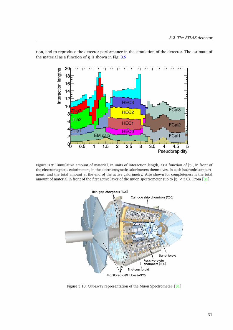
3.2 The ATLAS detector
tion, and to reproduce the detector performance in the simulation of the detector. The estimate ofthe material as a function of η is shown in Fig. 3.9.
0 0.5 1 1.5 2 2.5 3 3.5 4 4.5 502468
101214161820
Pseudorapidity0 0.5 1 1.5 2 2.5 3 3.5 4 4.5 5
Inte
ract
ion
leng
ths
02468
101214161820
EM caloTile1
Tile2
Tile3
HEC0HEC1
HEC2
HEC3
FCal1
FCal2
FCal3
Figure 3.9: Cumulative amount of material, in units of interaction length, as a function of |η|, in front ofthe electromagnetic calorimeters, in the electromagnetic calorimeters themselves, in each hadronic compart-ment, and the total amount at the end of the active calorimetry. Also shown for completeness is the totalamount of material in front of the first active layer of the muon spectrometer (up to |η|< 3.0). From [31].
Figure 3.10: Cut-away representation of the Muon Spectrometer. [31]
31
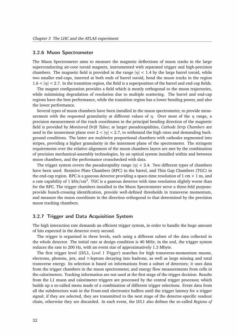
Chapter 3 The LHC and the ATLAS experiment
3.2.6 Muon Spectrometer
The Muon Spectrometer aims to measure the magnetic deflections of muon tracks in the largesuperconducting air-core toroid magnets, instrumented with separated trigger and high-precisionchambers. The magnetic field is provided in the range |η| < 1.4 by the large barrel toroid, whiletwo smaller end-caps, inserted at both ends of barrel toroid, bend the muon tracks in the region1.6< |η|< 2.7. In the transition region, the field is a superposition of the barrel and end-cap fields.
The magnet configuration provides a field which is mostly orthogonal to the muon trajectories,while minimising degradation of resolution due to multiple scattering. The barrel and end-capregions have the best performance, while the transition region has a lower bending power, and alsothe lower performance.
Several types of muon chambers have been installed in the muon spectrometer, to provide meas-urement with the requested granularity at different values of η. Over most of the η range, aprecision measurement of the track coordinates in the principal bending direction of the magneticfield is provided by Monitored Drift Tubes; at larger pseudorapidities, Cathode Strip Chambers areused in the innnermost plane over 2 < |η| < 2.7, to withstand the high rates and demanding back-ground conditions. The latter are multiwire proportional chambers with cathodes segmented intostripes, providing a higher granularity in the innermost plane of the spectrometer. The stringentrequirements over the relative alignment of the muon chambers layers are met by the combinationof precision mechanical-assembly technologies, by an optical system installed within and betweenmuon chambers, and the performance crosschecked with data.
The trigger system covers the pseudorapidity range |η| < 2.4. Two different types of chambershave been used: Resistive Plate Chambers (RPC) in the barrel, and Thin Gap Chambers (TGC) inthe end-cap region. RPC is a gaseous detector providing a space-time resolution of 1 cm × 1 ns, anda rate capability of 1 kHz/cm2. TGC is a gaseous detector with time resolution slightly worse thanfor the RPC. The trigger chambers installed in the Muon Spectrometer serve a three-fold purpose:provide bunch-crossing identification, provide well-defined thresholds in transverse momentum,and measure the muon coordinate in the direction orthogonal to that determined by the precisionmuon tracking chambers.
3.2.7 Trigger and Data Acquisition System
The high interaction rate demands an efficient trigger system, in order to handle the huge amountof hits expected in the detector every second.
The trigger is organised in three levels, each using a different subset of the data collected inthe whole detector. The initial rate at design condition is 40 MHz; in the end, the trigger systemreduces the rate to 200 Hz, with an event size of approximatively 1.3 Mbyte.
The first trigger level (LVL1, Level 1 Trigger) searches for high transverse-momentum muons,electrons, photons, jets, and τ-leptons decaying into hadrons, as well as large missing and totaltransverse energy. Its selection is based on informations from a subset of detectors; it uses datafrom the trigger chambers in the muon spectrometer, and energy flow measurements from cells inthe calorimeters. Tracking information are not used at the first stage of the trigger decision. Resultsfrom the L1 muon and calorimeter triggers are processed by the central trigger processor, whichbuilds up a so-called menu made of a combination of different trigger selections. Event data fromall the subdetectors wait in the Front-end electronics buffers until the trigger latency for a triggersignal; if they are selected, they are transmitted to the next stage of the detector-specific readoutchain, otherwise they are discarded. In each event, the LVL1 also defines the so-called Regions of
32
3.2 The ATLAS detector
Interest (RoI), i.e. the coordinates in η and φ of those regions of the detector where its selectionprocess has identified interesting features. The RoI data includes also the information on the typeof interesting features, and the criteria passed (e.g. a threshold). The RoI data are used by thesubsequent trigger stage.
The LVL1 reduces the rate from about 1 GHz to approximatively 75 kHz, with a processing timeof less than 2.5µs.
The LVL2 selection is seeded by the RoI information. LVL2 uses all the available detector datawithin the RoI (approximatively 2% of the total event data). This second stage reduced the rate toapproximatively 3.5 kHz, with an event processing time of about 40 ms.
The final stage is the event filter (EF), which reduces the rate to roughly 200 Hz. Its selectionsare implemented using offline analysis procedures, with an average processing time of the order offour seconds.
3.2.8 Simulation of the ATLAS detector
The GEANT4 software toolkit [34] within the simulation framework [32] propagates the generatedparticles through the detector and simulates their interactions with the detector material. Theenergy deposited by particles in the active detector material is converted into detector signals withthe same format as the detector read-out. The simulated detector signals are in turn reconstructedwith the same reconstruction software as used for the data.
In GEANT4 the model for the interaction of hadrons with the detector material can be specified forvarious particle types and for various energy ranges. For the simulation of hadronic interactions inthe detector, the GEANT4 set of processes called QGSP_BERT is chosen [3]. In this set of processes,the Quark Gluon String model [35, 36, 46, 47, 62] is used for the fragmentation of the nucleus,and the Bertini cascade model [43, 71, 77] for the description of the interactions of hadrons in thenuclear medium.
The GEANT4 simulation and in particular the hadronic interaction model for pions and protons,has been validated with test-beam measurements for the barrel and endcap calorimeters. Agree-ment within a few percent is found between simulation and data for pion momenta between 2 GeVand 350 GeV.
Further tests have been carried out in-situ comparing the single hadron response, measuredusing isolated tracks and identified single particles. Agreement within a few percent is found forthe inclusive measurement [5, 26] and for identified pions and protons from the decay productsof kaon and lambda particles produced in proton-proton collisions at 7 TeV [25]. With this methodparticle momenta of pions and protons in the range from a few hundred MeV to 6 GeV can bereached. Good agreement between Monte Carlo simulation and data is found.
33

Chapter 4
Jet Algorithms in VBF Higgs searches
The most likely interaction expected in pp collisions at the LHC is parton scattering. Quantumchromo-dynamics (QCD) predicts that no free partons can exist in nature: only colourless particlescan be expected in the final state, as explained in Sect. 2.2.2. Thus, the most likely final state to beobserved in the detectors will show several hadrons, produced from the original parton interactionvia hadronisation.
The hadrons detected in the final state carry the information about the hard scattering, but it isnot trivial to extract it. The number and kind of particles that are detected in the final state mightvary even if they originate from the same kind of parton interaction. To recover the link betweenthe partons and the particles in the final state, it is useful to define a clustering algorithm (calledjet algorithm): the output of such a procedure is a “macroscopic object”, called a jet, that aims todescribe the energy and kinematics of the partons in the final state. In theoretical calculations, a jetwill be either a single parton (at the parton level), or made of several partons (after fragmentation)or hadrons (after hadronisation); in an experiment, it will be reconstructed from detector signals,or computed back at hadron or parton level using Monte Carlo methods (unfolding).
Jets are not real physical objects: they acquire a precise meaning only after an algorithm hasbeen defined. Different definitions would produce different arrangements of the particles in thefinal states, and all of them are equally justified. As the jets carry fundamental information (thelink to the partons), their representation of the interaction should be equivalent; however, thedetailed implementation and definition depend also on the physics case, and different algorithmscould provide a worse or better representation of different partonic final states.
The definition of a jet has been widely studied in the past[78] and the characteristics that havebeen agreed upon will be summarized in Sect. 4.1. In Sect. 4.2 the algorithms used in ATLAS will bereviewed. In particular, in the context of VBF Higgs searches the performances of the jet algorithmsplay an important role, as the possibility to detect and distinguish this production mechanism relieson jet reconstruction. The results obtained from the investigation of different jet algorithms insimulations of VBF Higgs events in ATLAS will be reported in Sect. 4.3.
4.1 What is a jet?
A good jet algorithm definition should allow a comparison between the theoretical and the experi-mental level, as well as between different experimental results. The so-called Snowmass accord[78]is the output of a discussion among theorists and experimentalists, aimed at defining a commonground for all high pT QCD studies. According to it, a jet algorithm should:
• be simple to implement (both in a theoretical calculation and in an experimental measure-ment);
35
Chapter 4 Jet Algorithms in VBF Higgs searches
• be defined at any order in perturbation theory;
• yield finite cross section at any order of perturbation theory;
• yield a cross section that is relatively independent from hadronization.
The first condition requires the definition to be sufficiently general to be implemented, such thatjet objects can be defined both at theoretical and experimental level. The second condition ensuresthat those jets can be compared with each other, because they are well defined regardless of theorder considered for the calculation.
The third condition deals with the collinear and infrared safety. In both cases, the requirementfor the algorithm is to be independent of variables that would lead to divergences when consideredat a finite perturbative order.
The collinear unsafety arises when the jet algorithm makes a difference between two masslesscollinear particles and one single massless particle with energy equal to the combined energy ofthe former pair. In perturbative QCD, the cross section for the pair at a fixed order is divergent, butin the total cross section the divergence is cancelled by the contribution of the virtual correction atthe vertex, consisting in a single particle with momentum equal to the combined momentum. If thealgorithm does not respect this indifference, and instead represents these two cases differently, it isnot collinear safe.
The infrared unsafety occurs when the algorithm is sensitive to soft radiation emission. In per-turbative calculation, soft emission causes a divergence at low energy; this divergence is cancelledin the total cross section after renormalisation. If an algorithm is sensitive to these emissions, whichcould form for example new jets in the final state, the event description is not physical anymore,and the algorithm is infrared unsafe.
The last requirement states that the description of the event given by a jet algorithm should bemostly dependent on the primary partons, and only weakly on fragmentation and hadronization.This ensures that the global characteristics of the event depend largely on the partonic final state.
A jet algorithm which follows the Snowmass accord provides a link between the detector finalstate and the partonic final state as schematically represented in Fig. 4.1.
The main jet algorithms can be divided into two classes:
• Cone algorithms: define jets as the combination of input objects within a cone of radius Raround the jet direction. The jet direction is the one that maximizes the energy flow throughthe cone. Objects belong to the jet if their distance (in η,φ) is smaller than the cone radius.The four-momentum of the jet is computed using the energy of all the particles inside thecone, using conventional recombination schemes1. The cone radius can be optimized tominimize experimental effects.
The regions of maximum energy flow can be defined in different ways, and this can be apotential drawback for this class of algorithms. To avoid this problem, the jets are built usingan iterative procedure. Once the initial cone direction is defined, the energy-weighted central
1The most common recombination schemes are the “E” scheme, that adds the four vectors, and the “pT” scheme, whereeach added quantity is weighted by the pT of the particle. In the pT scheme, for example:
ET i j = ET i + ET j ηi j =ET iηi + ET jη j
ET i jφi j =
ET iφi + ET jφ j
ET i j
that is equivalent to the simple vector sum if the opening angle between i and j is small.
36
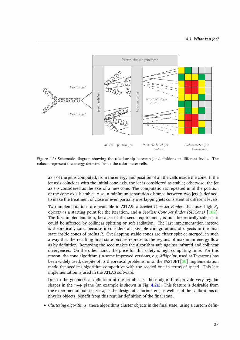
4.1 What is a jet?
Parton jet
Parton jet
Multi− parton jet Particle level jet Calorimeter jet(hadrons) (detector level)
K±, π±,K0, π0, p, n . . .
e±, µ±, ν . . .
Parton shower generator
fragm
entation
hadronization
Figure 4.1: Schematic diagram showing the relationship between jet definitions at different levels. Thecolours represent the energy detected inside the calorimeter cells.
axis of the jet is computed, from the energy and position of all the cells inside the cone. If thejet axis coincides with the initial cone axis, the jet is considered as stable; otherwise, the jetaxis is considered as the axis of a new cone. The computation is repeated until the positionof the cone axis is stable. Also, a minimum separation distance between two jets is defined,to make the treatment of close or even partially overlapping jets consistent at different levels.
Two implementations are available in ATLAS: a Seeded Cone Jet Finder, that uses high ETobjects as a starting point for the iteration, and a Seedless Cone Jet finder (SISCone) [102].The first implementation, because of the seed requirement, is not theoretically safe, as itcould be affected by collinear splitting or soft radiation. The last implementation insteadis theoretically safe, because it considers all possible configurations of objects in the finalstate inside cones of radius R. Overlapping stable cones are either split or merged, in sucha way that the resulting final state picture represents the regions of maximum energy flowas by definition. Removing the seed makes the algorithm safe against infrared and collineardivergences. On the other hand, the price for this safety is high computing time. For thisreason, the cone algorithm (in some improved versions, e.g. Midpoint, used at Tevatron) hasbeen widely used, despite of its theoretical problems, until the FASTJET[50] implementationmade the seedless algorithm competitive with the seeded one in terms of speed. This lastimplementation is used in the ATLAS software.
Due to the geometrical definition of the jet objects, those algorithms provide very regularshapes in the η–φ plane (an example is shown in Fig. 4.2a). This feature is desirable fromthe experimental point of view, as the design of calorimeters, as well as of the calibrations ofphysics objects, benefit from this regular definition of the final state.
• Clustering algorithms: these algorithms cluster objects in the final state, using a custom defin-
37
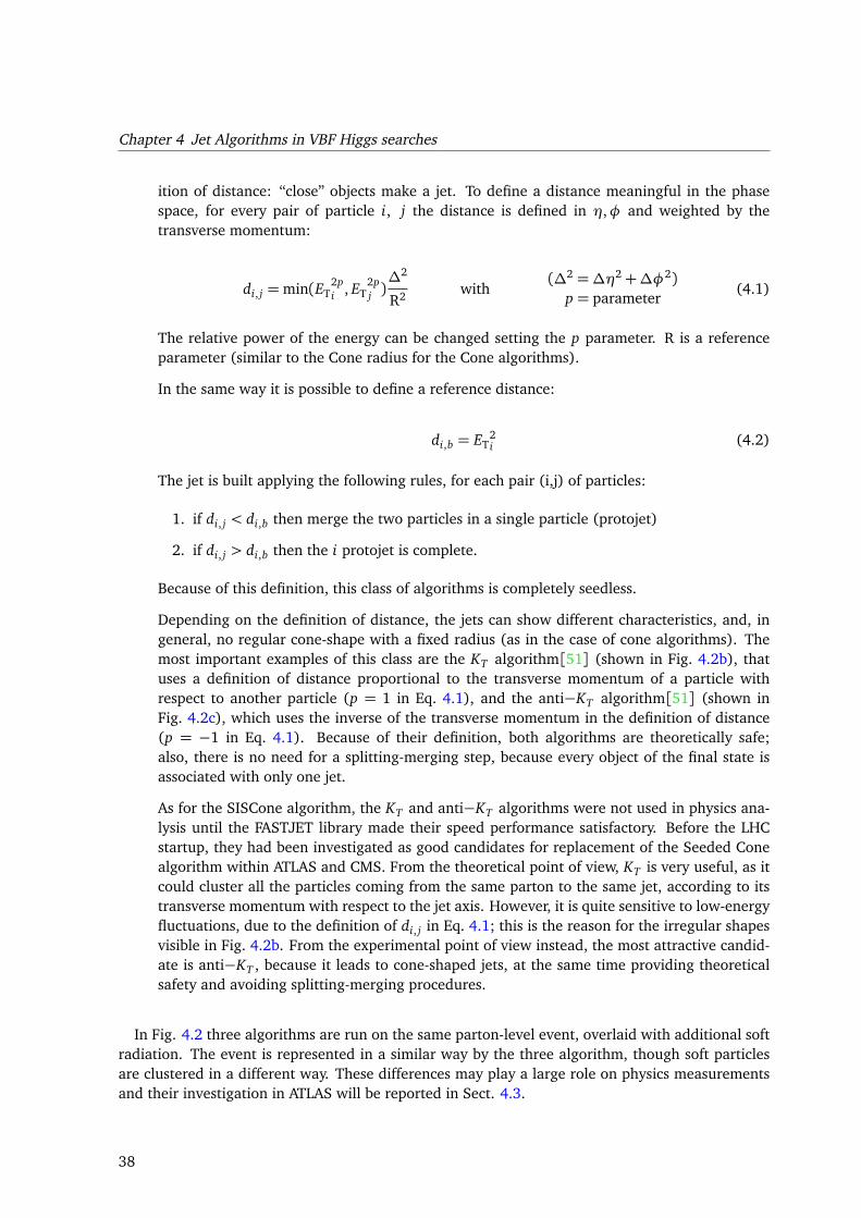
Chapter 4 Jet Algorithms in VBF Higgs searches
ition of distance: “close” objects make a jet. To define a distance meaningful in the phasespace, for every pair of particle i, j the distance is defined in η,φ and weighted by thetransverse momentum:
di, j =min(ET2pi , ET
2pj )∆2
R2 with(∆2 =∆η2+∆φ2)
p = parameter(4.1)
The relative power of the energy can be changed setting the p parameter. R is a referenceparameter (similar to the Cone radius for the Cone algorithms).
In the same way it is possible to define a reference distance:
di,b = ET2i (4.2)
The jet is built applying the following rules, for each pair (i,j) of particles:
1. if di, j < di,b then merge the two particles in a single particle (protojet)
2. if di, j > di,b then the i protojet is complete.
Because of this definition, this class of algorithms is completely seedless.
Depending on the definition of distance, the jets can show different characteristics, and, ingeneral, no regular cone-shape with a fixed radius (as in the case of cone algorithms). Themost important examples of this class are the KT algorithm[51] (shown in Fig. 4.2b), thatuses a definition of distance proportional to the transverse momentum of a particle withrespect to another particle (p = 1 in Eq. 4.1), and the anti−KT algorithm[51] (shown inFig. 4.2c), which uses the inverse of the transverse momentum in the definition of distance(p = −1 in Eq. 4.1). Because of their definition, both algorithms are theoretically safe;also, there is no need for a splitting-merging step, because every object of the final state isassociated with only one jet.
As for the SISCone algorithm, the KT and anti−KT algorithms were not used in physics ana-lysis until the FASTJET library made their speed performance satisfactory. Before the LHCstartup, they had been investigated as good candidates for replacement of the Seeded Conealgorithm within ATLAS and CMS. From the theoretical point of view, KT is very useful, as itcould cluster all the particles coming from the same parton to the same jet, according to itstransverse momentum with respect to the jet axis. However, it is quite sensitive to low-energyfluctuations, due to the definition of di, j in Eq. 4.1; this is the reason for the irregular shapesvisible in Fig. 4.2b. From the experimental point of view instead, the most attractive candid-ate is anti−KT , because it leads to cone-shaped jets, at the same time providing theoreticalsafety and avoiding splitting-merging procedures.
In Fig. 4.2 three algorithms are run on the same parton-level event, overlaid with additional softradiation. The event is represented in a similar way by the three algorithm, though soft particlesare clustered in a different way. These differences may play a large role on physics measurementsand their investigation in ATLAS will be reported in Sect. 4.3.
38
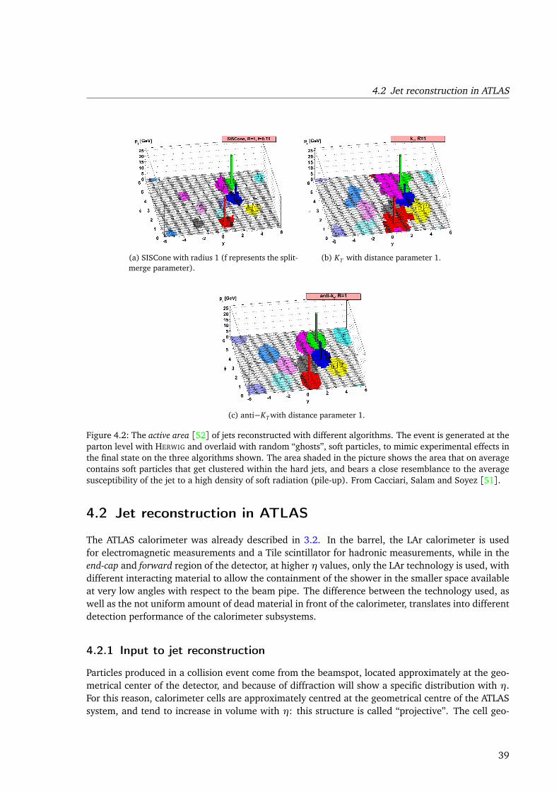
4.2 Jet reconstruction in ATLAS
(a) SISCone with radius 1 (f represents the split-merge parameter).
(b) KT with distance parameter 1.
(c) anti−KT with distance parameter 1.
Figure 4.2: The active area [52] of jets reconstructed with different algorithms. The event is generated at theparton level with HERWIG and overlaid with random “ghosts”, soft particles, to mimic experimental effects inthe final state on the three algorithms shown. The area shaded in the picture shows the area that on averagecontains soft particles that get clustered within the hard jets, and bears a close resemblance to the averagesusceptibility of the jet to a high density of soft radiation (pile-up). From Cacciari, Salam and Soyez [51].
4.2 Jet reconstruction in ATLAS
The ATLAS calorimeter was already described in 3.2. In the barrel, the LAr calorimeter is usedfor electromagnetic measurements and a Tile scintillator for hadronic measurements, while in theend-cap and forward region of the detector, at higher η values, only the LAr technology is used, withdifferent interacting material to allow the containment of the shower in the smaller space availableat very low angles with respect to the beam pipe. The difference between the technology used, aswell as the not uniform amount of dead material in front of the calorimeter, translates into differentdetection performance of the calorimeter subsystems.
4.2.1 Input to jet reconstruction
Particles produced in a collision event come from the beamspot, located approximately at the geo-metrical center of the detector, and because of diffraction will show a specific distribution with η.For this reason, calorimeter cells are approximately centred at the geometrical centre of the ATLASsystem, and tend to increase in volume with η: this structure is called “projective”. The cell geo-
39
Chapter 4 Jet Algorithms in VBF Higgs searches
metry is projective in the barrel, and only pseudo-projective in the hadronic end-cap (HEC), due tothe compact size requirement for the detector. For the same reason, the forward calorimeter (FCal)is not projective, but the cells lie horizontally, to achieve a better performance in the very smallregion available to the detector.
The signal detected in the cells is then passed to the next step of the reconstruction. To feed thejet algorithm, three input objects have been defined:
• Calorimeter towers: projective regions in the η−φ plane, dimension 0.1× 0.1. In projectivecalorimeters, a tower is consistent with a cell or a group of cells. For the non projectivecalorimeters, the grid of towers is overlaid on the cell structure in η−φ, and the energy iscomputed from the cell energy times a weight that represents the fraction of the cell volumewithin the tower volume. Because of fluctuations in the pedestal of the signal, a tower canhave either positive or negative energy, the negative energies representing only electronicnoise.
• Topological clusters (topoclusters): three-dimensional topological calorimeter clusters [88]built from calorimeter cells. Each topocluster is built starting from a seed calorimeter cellwith |Ecell| > 4σ, where σ is the RMS of the electronic noise of the cell. Neighbouring cellsare iteratively added to the topocluster if they have |Ecell| > 2σ. Finally, an outer layer ofsurrounding cells is added. Because of the threshold, a cluster can’t show negative energies:the threshold selection suppresses electronic noise.
• Topological towers (topotowers): after the calorimeter signal is reconstructed in topoclusters,the grid of towers is overlaid to the cluster distribution and towers are built from the cellsinside the reconstructed topoclusters. The result are noise-suppressed towers. As for thetopoclusters, also topotowers are always of positive energy.
The standard inputs in ATLAS are the topoclusters and the topotowers (usually simply calledtowers). In this study, only topoclusters will be used.
As mentioned earlier, a jet can also be defined at the particle and parton level. Jet at particle levelare often compared to reconstructed jets, either to estimate the performance at the reconstructionlevel, or to extract the properties of an interaction by unfolding the measurement back to theparticle level. In ATLAS, the particle level jets are called Truth jets and built from simulated particlesafter parton shower. For these jets, all stable particles with proper lifetimes longer than 10 ps areconsidered (excluding muons and neutrinos).
4.3 Jet Algorithm studies in Vector-Boson-Fusion simulatedsamples
4.3.1 Motivation
In Aad et al. [9], the ATLAS analysis strategies for different physics cases are tested using simulateddata sets and the software framework designed for the data taking conditions. In that work, theATLAS standard algorithm used is the Cone Algorithm. After the publication, several alternativeswere proposed in theory papers, and, thanks to the development of the FASTJET code, could beimplemented in the ATLAS framework. A global effort started in ATLAS, in order to understandwhether a new algorithm could have provided better performance in the analysis than the standard
40
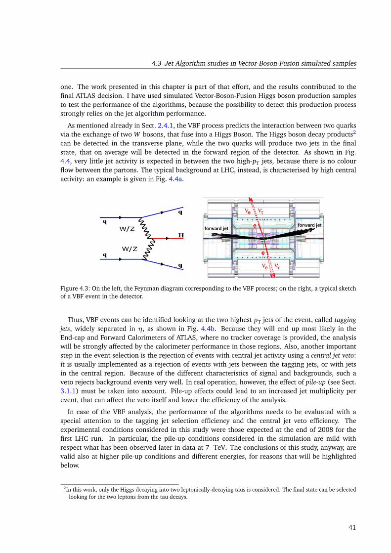
4.3 Jet Algorithm studies in Vector-Boson-Fusion simulated samples
one. The work presented in this chapter is part of that effort, and the results contributed to thefinal ATLAS decision. I have used simulated Vector-Boson-Fusion Higgs boson production samplesto test the performance of the algorithms, because the possibility to detect this production processstrongly relies on the jet algorithm performance.
As mentioned already in Sect. 2.4.1, the VBF process predicts the interaction between two quarksvia the exchange of two W bosons, that fuse into a Higgs Boson. The Higgs boson decay products2
can be detected in the transverse plane, while the two quarks will produce two jets in the finalstate, that on average will be detected in the forward region of the detector. As shown in Fig.4.4, very little jet activity is expected in between the two high-pT jets, because there is no colourflow between the partons. The typical background at LHC, instead, is characterised by high centralactivity: an example is given in Fig. 4.4a.
Figure 4.3: On the left, the Feynman diagram corresponding to the VBF process; on the right, a typical sketchof a VBF event in the detector.
Thus, VBF events can be identified looking at the two highest pT jets of the event, called taggingjets, widely separated in η, as shown in Fig. 4.4b. Because they will end up most likely in theEnd-cap and Forward Calorimeters of ATLAS, where no tracker coverage is provided, the analysiswill be strongly affected by the calorimeter performance in those regions. Also, another importantstep in the event selection is the rejection of events with central jet activity using a central jet veto:it is usually implemented as a rejection of events with jets between the tagging jets, or with jetsin the central region. Because of the different characteristics of signal and backgrounds, such aveto rejects background events very well. In real operation, however, the effect of pile-up (see Sect.3.1.1) must be taken into account. Pile-up effects could lead to an increased jet multiplicity perevent, that can affect the veto itself and lower the efficiency of the analysis.
In case of the VBF analysis, the performance of the algorithms needs to be evaluated with aspecial attention to the tagging jet selection efficiency and the central jet veto efficiency. Theexperimental conditions considered in this study were those expected at the end of 2008 for thefirst LHC run. In particular, the pile-up conditions considered in the simulation are mild withrespect what has been observed later in data at 7 TeV. The conclusions of this study, anyway, arevalid also at higher pile-up conditions and different energies, for reasons that will be highlightedbelow.
2In this work, only the Higgs decaying into two leptonically-decaying taus is considered. The final state can be selectedlooking for the two leptons from the tau decays.
41
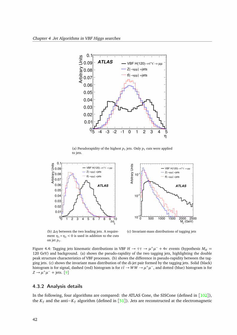
Chapter 4 Jet Algorithms in VBF Higgs searches
η-5 -4 -3 -2 -1 0 1 2 3 4 5
Arb
itra
ry U
nits
0
0.01
0.02
0.03
0.04
0.05
0.06
0.07
0.08
0.09
0.1
µµ →-τ+τ→VBF H(120)
) +jetsµµ→Z(
) +jetsµµ→(tt
ATLAS
(a) Pseudorapidity of the highest pT jets. Only pT cuts were appliedto jets.
jjη∆
0 1 2 3 4 5 6 7 8 9 10
Arb
itra
ry U
nits
0
0.01
0.02
0.03
0.04
0.05
0.06
0.07
0.08
0.09
0.1
µµ →-τ+τ→VBF H(120)
) +jetsµµ→Z(
) +jetsµµ→(tt
ATLAS
(b) ∆η between the two leading jets. A require-ment η1 ∗ η2 < 0 is used in addition to the cutson jet pT.
(GeV)jj
M0 500 1000 1500 2000 2500
Arb
itra
ry U
nits
-310
-210
-110
µµ →-τ+τ→VBF H(120)
) +jetsµµ→Z(
) +jetsµµ→(tt
ATLAS
(c) Invariant-mass distributions of tagging jets
Figure 4.4: Tagging jets kinematic distributions in VBF H → ττ → µ+µ− + 4ν events (hypothesis MH =120 GeV) and background. (a) shows the pseudo-rapidity of the two tagging jets, highlighting the doublepeak structure characteristics of VBF processes. (b) shows the difference in pseudo-rapidity between the tag-ging jets. (c) shows the invariant mass distribution of the di-jet pair formed by the tagging jets. Solid (black)histogram is for signal, dashed (red) histogram is for t t →WW → µ+µ−, and dotted (blue) histogram is forZ → µ+µ− + jets. [9]
4.3.2 Analysis details
In the following, four algorithms are compared: the ATLAS Cone, the SISCone (defined in [102]),the KT and the anti−KT algorithm (defined in [51]). Jets are reconstructed at the electromagnetic
42
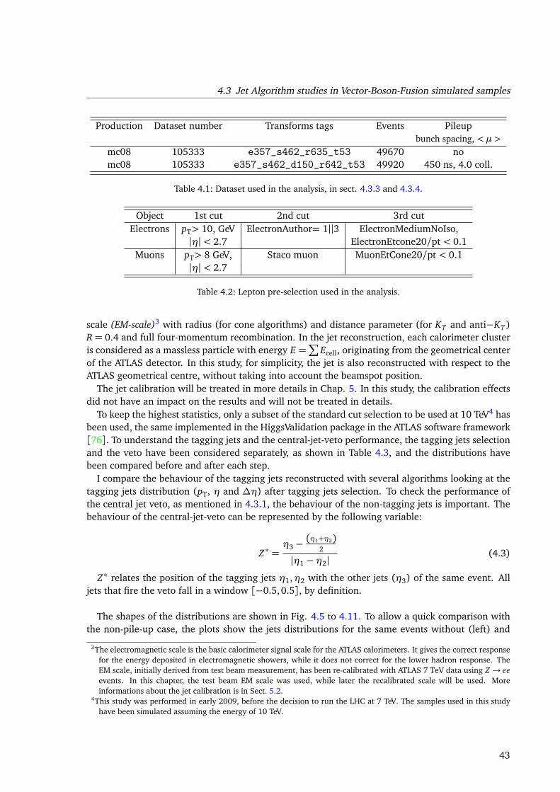
4.3 Jet Algorithm studies in Vector-Boson-Fusion simulated samples
Production Dataset number Transforms tags Events Pileupbunch spacing, < µ >
mc08 105333 e357_s462_r635_t53 49670 nomc08 105333 e357_s462_d150_r642_t53 49920 450 ns, 4.0 coll.
Table 4.1: Dataset used in the analysis, in sect. 4.3.3 and 4.3.4.
Object 1st cut 2nd cut 3rd cutElectrons pT> 10, GeV ElectronAuthor= 1||3 ElectronMediumNoIso,
|η|< 2.7 ElectronEtcone20/pt < 0.1Muons pT> 8 GeV, Staco muon MuonEtCone20/pt < 0.1
|η|< 2.7
Table 4.2: Lepton pre-selection used in the analysis.
scale (EM-scale)3 with radius (for cone algorithms) and distance parameter (for KT and anti−KT )R= 0.4 and full four-momentum recombination. In the jet reconstruction, each calorimeter clusteris considered as a massless particle with energy E =
∑
Ecell, originating from the geometrical centerof the ATLAS detector. In this study, for simplicity, the jet is also reconstructed with respect to theATLAS geometrical centre, without taking into account the beamspot position.
The jet calibration will be treated in more details in Chap. 5. In this study, the calibration effectsdid not have an impact on the results and will not be treated in details.
To keep the highest statistics, only a subset of the standard cut selection to be used at 10 TeV4 hasbeen used, the same implemented in the HiggsValidation package in the ATLAS software framework[76]. To understand the tagging jets and the central-jet-veto performance, the tagging jets selectionand the veto have been considered separately, as shown in Table 4.3, and the distributions havebeen compared before and after each step.
I compare the behaviour of the tagging jets reconstructed with several algorithms looking at thetagging jets distribution (pT, η and ∆η) after tagging jets selection. To check the performance ofthe central jet veto, as mentioned in 4.3.1, the behaviour of the non-tagging jets is important. Thebehaviour of the central-jet-veto can be represented by the following variable:
Z∗ =η3−
(η1+η2)2
|η1−η2|(4.3)
Z∗ relates the position of the tagging jets η1,η2 with the other jets (η3) of the same event. Alljets that fire the veto fall in a window [−0.5,0.5], by definition.
The shapes of the distributions are shown in Fig. 4.5 to 4.11. To allow a quick comparison withthe non-pile-up case, the plots show the jets distributions for the same events without (left) and
3The electromagnetic scale is the basic calorimeter signal scale for the ATLAS calorimeters. It gives the correct responsefor the energy deposited in electromagnetic showers, while it does not correct for the lower hadron response. TheEM scale, initially derived from test beam measurement, has been re-calibrated with ATLAS 7 TeV data using Z → eeevents. In this chapter, the test beam EM scale was used, while later the recalibrated scale will be used. Moreinformations about the jet calibration is in Sect. 5.2.
4This study was performed in early 2009, before the decision to run the LHC at 7 TeV. The samples used in this studyhave been simulated assuming the energy of 10 TeV.
43
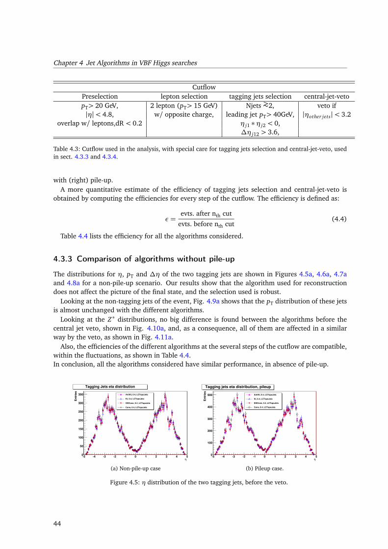
Chapter 4 Jet Algorithms in VBF Higgs searches
CutflowPreselection lepton selection tagging jets selection central-jet-vetopT> 20 GeV, 2 lepton (pT> 15 GeV) Njets ∼>2, veto if|η|< 4.8, w/ opposite charge, leading jet pT> 40GeV, |ηother jets|< 3.2
overlap w/ leptons,dR < 0.2 η j1 ∗η j2 < 0,∆η j12 > 3.6,
Table 4.3: Cutflow used in the analysis, with special care for tagging jets selection and central-jet-veto, usedin sect. 4.3.3 and 4.3.4.
with (right) pile-up.A more quantitative estimate of the efficiency of tagging jets selection and central-jet-veto is
obtained by computing the efficiencies for every step of the cutflow. The efficiency is defined as:
ε=evts. after nth cut
evts. before nth cut(4.4)
Table 4.4 lists the efficiency for all the algorithms considered.
4.3.3 Comparison of algorithms without pile-up
The distributions for η, pT and ∆η of the two tagging jets are shown in Figures 4.5a, 4.6a, 4.7aand 4.8a for a non-pile-up scenario. Our results show that the algorithm used for reconstructiondoes not affect the picture of the final state, and the selection used is robust.
Looking at the non-tagging jets of the event, Fig. 4.9a shows that the pT distribution of these jetsis almost unchanged with the different algorithms.
Looking at the Z∗ distributions, no big difference is found between the algorithms before thecentral jet veto, shown in Fig. 4.10a, and, as a consequence, all of them are affected in a similarway by the veto, as shown in Fig. 4.11a.
Also, the efficiencies of the different algorithms at the several steps of the cutflow are compatible,within the fluctuations, as shown in Table 4.4.In conclusion, all the algorithms considered have similar performance, in absence of pile-up.
η5 4 3 2 1 0 1 2 3 4 5
En
trie
s
0
50
100
150
200
250
300
350
Tagging Jets eta distribution
AntiKt, 0.4, LCTopoJets
Kt, 0.4, LCTopoJets
SISCone, 0.4, LCTopoJets
Cone, 0.4, LCTopoJets
(a) Non-pile-up case
η5 4 3 2 1 0 1 2 3 4 5
En
trie
s
0
100
200
300
400
500 AntiKt, 0.4, LCTopoJets
Kt, 0.4, LCTopoJets
SISCone, 0.4, LCTopoJets
Cone, 0.4, LCTopoJets
Tagging jets eta distribution, pileup
(b) Pileup case.
Figure 4.5: η distribution of the two tagging jets, before the veto.
44
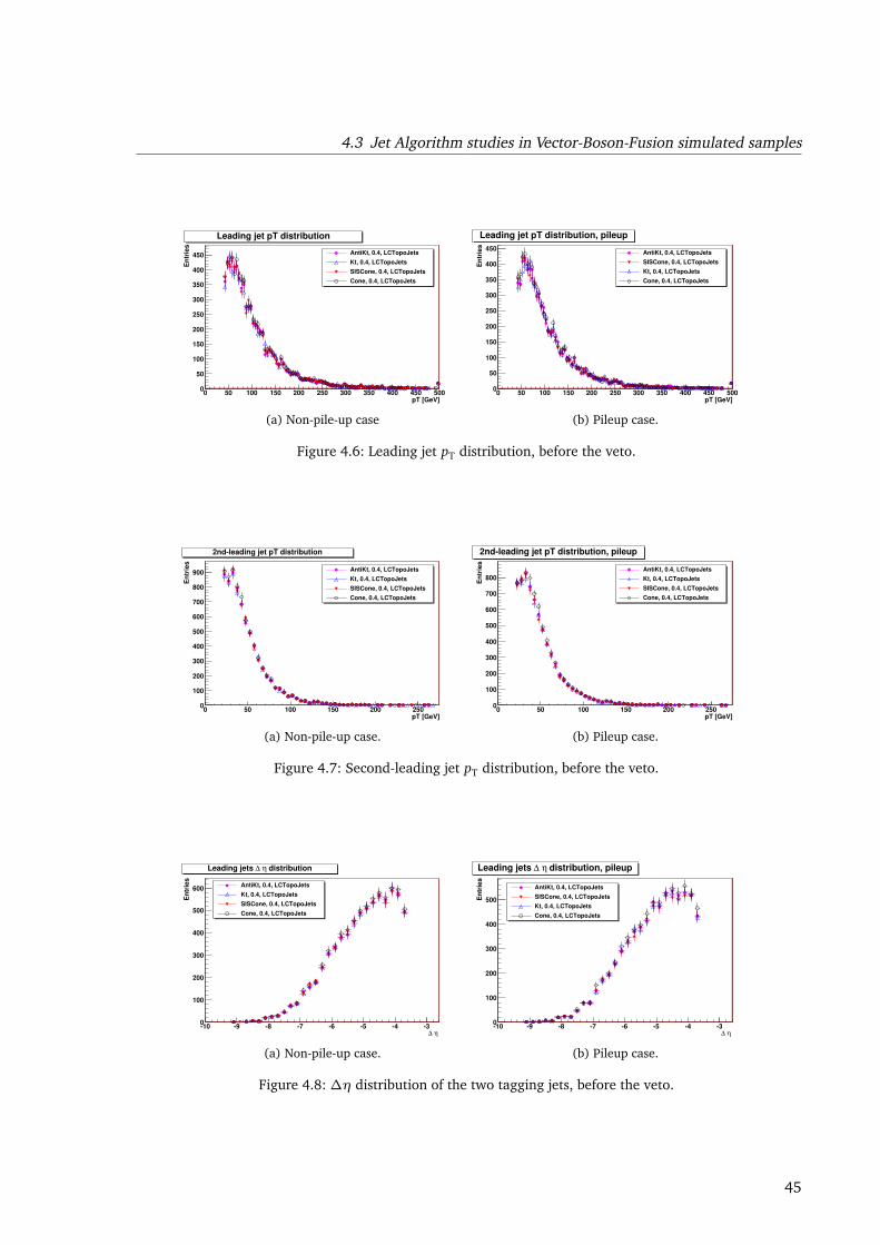
4.3 Jet Algorithm studies in Vector-Boson-Fusion simulated samples
pT [GeV]0 50 100 150 200 250 300 350 400 450 500
En
trie
s
0
50
100
150
200
250
300
350
400
450 AntiKt, 0.4, LCTopoJets
Kt, 0.4, LCTopoJets
SISCone, 0.4, LCTopoJets
Cone, 0.4, LCTopoJets
Leading jet pT distribution
(a) Non-pile-up case
pT [GeV]0 50 100 150 200 250 300 350 400 450 500
En
trie
s
0
50
100
150
200
250
300
350
400
450AntiKt, 0.4, LCTopoJets
SISCone, 0.4, LCTopoJets
Kt, 0.4, LCTopoJets
Cone, 0.4, LCTopoJets
Leading jet pT distribution, pileup
(b) Pileup case.
Figure 4.6: Leading jet pT distribution, before the veto.
pT [GeV]0 50 100 150 200 250
En
trie
s
0
100
200
300
400
500
600
700
800
900AntiKt, 0.4, LCTopoJets
Kt, 0.4, LCTopoJets
SISCone, 0.4, LCTopoJets
Cone, 0.4, LCTopoJets
2ndleading jet pT distribution
(a) Non-pile-up case.
pT [GeV]0 50 100 150 200 250
En
trie
s
0
100
200
300
400
500
600
700
800
AntiKt, 0.4, LCTopoJets
Kt, 0.4, LCTopoJets
SISCone, 0.4, LCTopoJets
Cone, 0.4, LCTopoJets
2ndleading jet pT distribution, pileup
(b) Pileup case.
Figure 4.7: Second-leading jet pT distribution, before the veto.
η ∆10 9 8 7 6 5 4 3
En
trie
s
0
100
200
300
400
500
600AntiKt, 0.4, LCTopoJets
Kt, 0.4, LCTopoJets
SISCone, 0.4, LCTopoJets
Cone, 0.4, LCTopoJets
distributionη ∆Leading jets
(a) Non-pile-up case.
η ∆10 9 8 7 6 5 4 3
En
trie
s
0
100
200
300
400
500
AntiKt, 0.4, LCTopoJets
SISCone, 0.4, LCTopoJets
Kt, 0.4, LCTopoJets
Cone, 0.4, LCTopoJets
distribution, pileupη ∆Leading jets
(b) Pileup case.
Figure 4.8: ∆η distribution of the two tagging jets, before the veto.
45
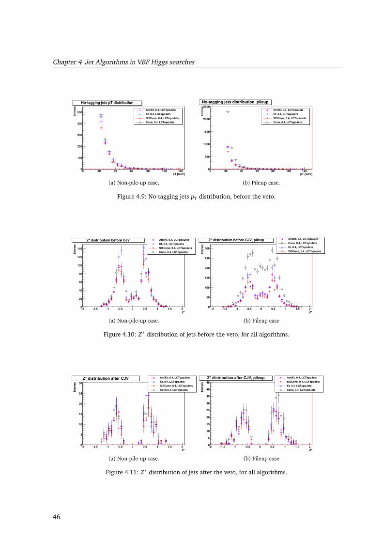
Chapter 4 Jet Algorithms in VBF Higgs searches
pT [GeV]0 20 40 60 80 100 120
En
trie
s
0
100
200
300
400
500AntiKt, 0.4, LCTopoJets
Kt, 0.4, LCTopoJets
SISCone, 0.4, LCTopoJets
Cone, 0.4, LCTopoJets
Notagging jets pT distribution
(a) Non-pile-up case.
pT [GeV]0 20 40 60 80 100 120
En
trie
s
0
500
1000
1500
2000
2500AntiKt, 0.4, LCTopoJets
Kt, 0.4, LCTopoJets
SISCone, 0.4, LCTopoJets
Cone, 0.4, LCTopoJets
Notagging jets distribution, pileup
(b) Pileup case.
Figure 4.9: No-tagging jets pT distribution, before the veto.
Z*2 1.5 1 0.5 0 0.5 1 1.5 2
En
trie
s
0
20
40
60
80
100
120
140
AntiKt, 0.4, LCTopoJets
Kt, 0.4, LCTopoJets
SISCone, 0.4, LCTopoJets
Cone, 0.4, LCTopoJets
Z* distribution before CJV
(a) Non-pile-up case.
Z*2 1.5 1 0.5 0 0.5 1 1.5 2
En
trie
s
0
50
100
150
200
250
300
AntiKt, 0.4, LCTopoJets
Cone, 0.4, LCTopoJets
Kt, 0.4, LCTopoJets
SISCone, 0.4, LCTopoJets
Z* distribution before CJV, pileup
(b) Pileup case
Figure 4.10: Z∗ distribution of jets before the veto, for all algorithms.
Z*2 1.5 1 0.5 0 0.5 1 1.5 2
En
trie
s
0
5
10
15
20
25
30
AntiKt, 0.4, LCTopoJets
Kt, 0.4, LCTopoJets
SISCone, 0.4, LCTopoJets
Cone,0.4, LCTopoJets
Z* distribution after CJV
(a) Non-pile-up case.
Z*2 1.5 1 0.5 0 0.5 1 1.5 2
En
trie
s
0
5
10
15
20
25
30
35
40
45
AntiKt, 0.4, LCTopoJets
SISCone, 0.4, LCTopoJets
Kt, 0.4, LCTopoJets
Cone, 0.4, LCTopoJets
Z* distribution after CJV, pileup
(b) Pileup case
Figure 4.11: Z∗ distribution of jets after the veto, for all algorithms.
46
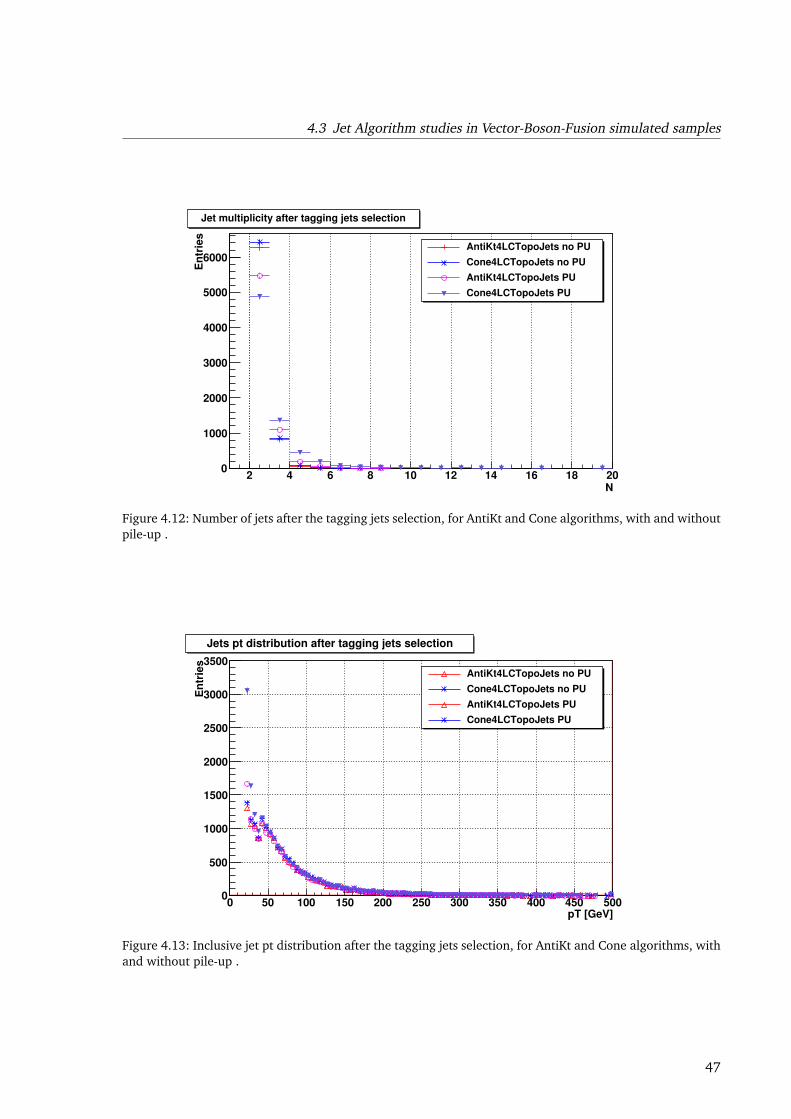
4.3 Jet Algorithm studies in Vector-Boson-Fusion simulated samples
N2 4 6 8 10 12 14 16 18 20
En
trie
s
0
1000
2000
3000
4000
5000
6000
Jet multiplicity after tagging jets selection
AntiKt4LCTopoJets no PU
Cone4LCTopoJets no PU
AntiKt4LCTopoJets PU
Cone4LCTopoJets PU
Figure 4.12: Number of jets after the tagging jets selection, for AntiKt and Cone algorithms, with and withoutpile-up .
pT [GeV]0 50 100 150 200 250 300 350 400 450 500
En
trie
s
0
500
1000
1500
2000
2500
3000
3500AntiKt4LCTopoJets no PU
Cone4LCTopoJets no PU
AntiKt4LCTopoJets PU
Cone4LCTopoJets PU
Jets pt distribution after tagging jets selection
Figure 4.13: Inclusive jet pt distribution after the tagging jets selection, for AntiKt and Cone algorithms, withand without pile-up .
47
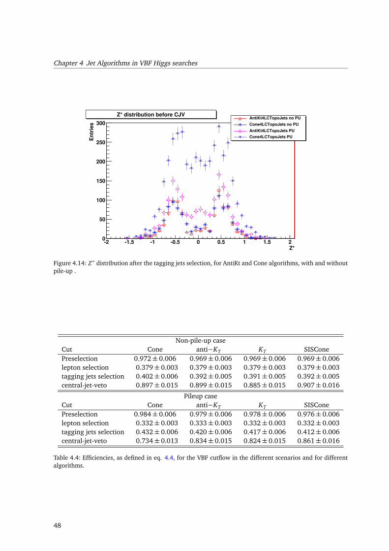
Chapter 4 Jet Algorithms in VBF Higgs searches
Z*2 1.5 1 0.5 0 0.5 1 1.5 2
En
trie
s
0
50
100
150
200
250
300AntiKt4LCTopoJets no PU
Cone4LCTopoJets no PU
AntiKt4LCTopoJets PU
Cone4LCTopoJets PU
Z* distribution before CJV
Figure 4.14: Z∗ distribution after the tagging jets selection, for AntiKt and Cone algorithms, with and withoutpile-up .
Non-pile-up caseCut Cone anti−KT KT SISConePreselection 0.972± 0.006 0.969± 0.006 0.969± 0.006 0.969± 0.006lepton selection 0.379± 0.003 0.379± 0.003 0.379± 0.003 0.379± 0.003tagging jets selection 0.402± 0.006 0.392± 0.005 0.391± 0.005 0.392± 0.005central-jet-veto 0.897± 0.015 0.899± 0.015 0.885± 0.015 0.907± 0.016
Pileup caseCut Cone anti−KT KT SISConePreselection 0.984± 0.006 0.979± 0.006 0.978± 0.006 0.976± 0.006lepton selection 0.332± 0.003 0.333± 0.003 0.332± 0.003 0.332± 0.003tagging jets selection 0.432± 0.006 0.420± 0.006 0.417± 0.006 0.412± 0.006central-jet-veto 0.734± 0.013 0.834± 0.015 0.824± 0.015 0.861± 0.016
Table 4.4: Efficiencies, as defined in eq. 4.4, for the VBF cutflow in the different scenarios and for differentalgorithms.
48
4.4 Conclusions
4.3.4 Comparison of algorithms with pile-up
The expected behavior in the pile-up case is a higher jet multiplicity per event, as shown in Fig.4.12. Also other distributions could be affected by the increased activity per event. An example ofthe differences between the non-pile-up and the pile-up case is shown in fig. 4.13 and 4.14, for twoof the considered algorithms.
The tagging jet distributions don’t show big differences between the algorithms, as shown in fig4.6b and 4.7b.
Looking at the non-tagging jets distributions, the differences get bigger. From the inclusive pTspectrum (Fig. 4.13), the increased jet multiplicity is shown to consist mostly of jets at low pT; thesecond peak visible in the distribution, caused by the pjet
T cut on the leading jet at 40 GeV, is almost
unaffected by the pile-up. The increase at low pjetT is much higher for the Cone algorithm than for
the other algorithms, as shown in fig. 4.9b. Also from the Z∗ distribution (Fig. 4.10b), is shownthat these jets can enhance the probability to fire the veto, because the Z∗ distribution around 0 ismore populated for the Cone algorithm. All the other algorithms show some differences, but theirdistributions are compatible within statistical fluctuations, hint that their representation of the finalstate is robust against pile-up.
The higher probability to fire the jet veto is reflected in the efficiencies reported in Table 4.4: theCone algorithm shows a large efficiency drop in the pile-up scenario with respect to the non-pile-upcase, and it is not compatible with the results from the other algorithms. This behaviour stronglydiscourages the use of the Cone algorithm in the analysis, in favour of the other infrared-collinearsafe algorithms.
The behaviour observed is interpreted as a combined effect of the splitting-merging procedureand the intrinsic unsafety of the Cone algorithm. It seems likely that in some configurations theCone algorithm splits one of the tagging jets into two or three jets: one of them still at high pT, withalmost no effect on the leading jets distributions, and the others at lower pT, but still sometimesabove the 20 GeV cut used in the jet selection. These additional jets will lie very close to the leadingjets, and in some cases exactly inside the rapidity gap: in this case, the event will fire the veto. Sucha behavior is an example of infrared unsafety. An example of such an event is shown in Fig. 4.15.In the event display with the Cone algorithm (Fig. 4.15b and 4.15d), two additional low-pT jets arereconstructed, and one of them (labeled “4” in the picture) is very close to one of the tagging jets(labeled “1”). As the event display shows, those additional reconstructed jets can fall within therapidity gap; thus the higher probability to fire the veto.
4.4 Conclusions
I have shown the results of the validation of the VBF analysis with respect to jet algorithms withsimulated ATLAS data at 10 TeV. Some issues have been identified, already considering even onlya very mild pile-up scenario. The results on the analysis using the Cone algorithm are not robustagainst pile-up; in the VBF case, this algorithm is less efficient than other algorithms after a centraljet veto is applied, making this rejection technique less effective in enhancing the sensitivity to thesignal. The other available infrared-collinear safe algorithms show no such behaviour, both withand without pile-up. Because the pile-up scenario considered is very mild in comparison to whathas been already observed at LHC, this study strongly discourages the usage of the Cone algorithmin LHC physics analyses. The anti−KT , KT and SISCone algorithms, meet the needs of the Higgsanalysis designed for the VBF channel in ATLAS.
49
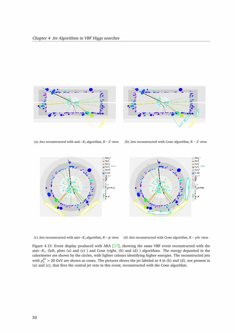
Chapter 4 Jet Algorithms in VBF Higgs searches
(a) Jets reconstructed with anti−KT algorithm, R−Z view. (b) Jets reconstructed with Cone algorithm, R− Z view.
(c) Jets reconstructed with anti−KT algorithm, R−φ view. (d) Jets reconstructed with Cone algorithm, R− phi view.
Figure 4.15: Event display produced with ARA [37], showing the same VBF event reconstructed with theanti−KT (left, plots (a) and (c) ) and Cone (right, (b) and (d) ) algorithms. The energy deposited in thecalorimeter are shown by the circles, with lighter colours identifying higher energies. The reconstructed jetswith pjet
T > 20 GeV are shown as cones. The pictures shows the jet labeled as 4 in (b) and (d), not present in(a) and (c), that fires the central jet veto in this event, reconstructed with the Cone algorithm.
50
Chapter 5
Jet η-intercalibration in 2010 data atps = 7 TeV
5.1 Strategy
The first ATLAS data collected at 7 TeV centre of mass energy have been used to establish theperformance of the detector. From the point of view of jet reconstruction, the data provided a largesample to establish the performance of the jet algorithm and of the jet energy scale calibration (aswell as the trigger performance[23], which will not be discussed). The strategy for 2010 data wasdesigned as follows:
1. compare EM-scale jet properties observed in data with their description by simulation samples,looking at calorimeter variables, for validation purposes;
2. understand the non-collision backgrounds, effects expected to be not reproduced by the si-mulations used in the early data comparison;
3. validate the jet reconstruction and calibration performance using a preliminary jet energyscale calibration, based on test beam detector studies and simulations; after validation, re-derive the jet energy scale calibration for the full 2010 dataset: the baseline calibration de-rived from simulation, the pile-up effects estimated from data (see Sect. 5.2.2);
4. use in-situ calibrations in data to perform a cross-check of the final jet energy scale (see Sect.5.3).
In-situ calibrations are methods that permit to test or derive the energy calibration taking thereference and the object to be calibrated from the same dataset. The η-intercalibration is one ofthem: it consists in a tag-and-probe analysis in di-jet events, where one jet is considered as a re-ference and the other one is calibrated with respect to the reference. This calibration is designedto understand the jet energy scale in the entire calorimeter, and is thus of fundamental importancefor measurements with jet final states. In particular, the η-intercalibration is important to calibratethe forward region, where the measurement from the calorimeter can’t be cross-checked with mea-surements coming from other detectors. The challenges in describing and calibrating the differentsections of the calorimeter will be summarized in Sect. 5.2.2.
The results obtained in 2010 are summarised in Aad et al. [10]. I have contributed to the ATLASpublication, focussing on the η-intercalibration. This has been the first attempt to understand theenergy scale in the forward region, and reached already very good results with 35 pb−1. The detailsof the analysis will be treated in Sect. 5.3. Results and open issues will be reviewed in Sect. 5.3.4.These results have been used to estimate the jet energy scale uncertainty in the forward region ofthe detector, as will be summarized in Sect. 5.3.4.
51
Chapter 5 Jet η-intercalibration in 2010 data atp
s = 7 TeV
5.2 Jet energy scale calibration
5.2.1 Hadronic showers in a calorimeter
The definition of a jet has been explained in 4.1. In experiments, a jet is commonly built from de-tector measurements. The experimental input objects to the jet algorithm are tracks or calorimetersignals. We will focus on the second case in our analysis.
To detect the energy of a particle, the calorimeters use the principle of the energy loss in matter:a particle, during its passage, looses energy according to its charge, type, speed, and the stoppingpower of the material[84]. In addition, in case of hadronic particles also the probability of nuclearinteractions with the nuclei of the material must be considered. If it is possible to measure theenergy absorbed by the material, this corresponds to the energy of the particle at the entrance ofthe material itself.
The ATLAS calorimeter system consists of sampling calorimeters. A sampling calorimeter usestwo types of material: a passive one, usually with high atomic number or with a high probabilityfor nuclear interactions with hadronic particles, and an active material, with lower atomic numberand able to detect a signal that is proportional to the energy of the particle (ionization in LAr andscintillation in Tile; see Sect. 3.2). The material is arranged in layers along the particle direction,such that each particle will pass through several layers of active and passive material. In each layer,the particle will loose energy as a result of the interaction with the material: at high energies theinteraction will result in the production of additional particles with lower energies, from eitherhadronic interactions with nuclei, or pair production for photons, or bremsstrahlung for electrons;at lower energies, ionization and excitation of the atoms of the material become the dominantprocesses, and the production of additional particles does not occur anymore. The global process,from the entrance of the initial particle in the calorimeter to the thermalization of all producedparticles in the material produces a so-called “shower particle” [113], as it is schematically shownin Fig. 5.1 for several particles. The kinetic energy of the incident particle is transferred to theshower particle, according to the interactions responsible for the process, and to the characteristicsof the detector (not only the atomic numbers of the active and passive materials, but also theirthickness, for example). In the active layers, the energy of the shower particle is sampled bymeasuring the energy deposited by the particles inside the shower, and this permits to reconstructthe energy of the initial particle.
Because the detection is based on the energy lost, the energy measurement has to take intoaccount both the kind of interaction between the particle and the absorber, and the particle massand energy. Some of the particles produced in the hard interaction and after hadronization willhave a lifetime long enough to reach the calorimeter: protons, neutrons, pions and K mesons,photons and leptons.
For muons, calorimeters are not an efficient detector, because muons release only little energy inthe layers. On the other hand, the presence of muons in a hadronic shower particle (where theycould be produced by decays in flight) is negligible with respect to the global composition of theshower.
Electrons and photons loose energy via electromagnetic interaction. Photons mostly producee+e− pairs or interact via compton scattering (for moderate energies of the incident photon), whileelectrons radiate other photons via bremstrahlung. This creates an electromagnetic shower in thecalorimeter. An electromagnetic shower is a relatively simple object: it is made only of electrons andphotons, and as it depends only on quantum electrodynamics, its characteristics can be computedwith a high accuracy. The shower develops quickly and in a small space, producing a very dense
52
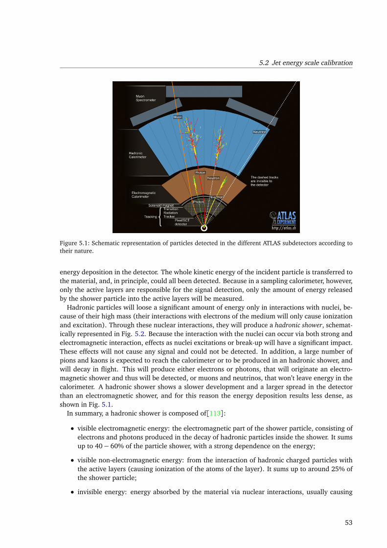
5.2 Jet energy scale calibration
Figure 5.1: Schematic representation of particles detected in the different ATLAS subdetectors according totheir nature.
energy deposition in the detector. The whole kinetic energy of the incident particle is transferred tothe material, and, in principle, could all been detected. Because in a sampling calorimeter, however,only the active layers are responsible for the signal detection, only the amount of energy releasedby the shower particle into the active layers will be measured.
Hadronic particles will loose a significant amount of energy only in interactions with nuclei, be-cause of their high mass (their interactions with electrons of the medium will only cause ionizationand excitation). Through these nuclear interactions, they will produce a hadronic shower, schemat-ically represented in Fig. 5.2. Because the interaction with the nuclei can occur via both strong andelectromagnetic interaction, effects as nuclei excitations or break-up will have a significant impact.These effects will not cause any signal and could not be detected. In addition, a large number ofpions and kaons is expected to reach the calorimeter or to be produced in an hadronic shower, andwill decay in flight. This will produce either electrons or photons, that will originate an electro-magnetic shower and thus will be detected, or muons and neutrinos, that won’t leave energy in thecalorimeter. A hadronic shower shows a slower development and a larger spread in the detectorthan an electromagnetic shower, and for this reason the energy deposition results less dense, asshown in Fig. 5.1.
In summary, a hadronic shower is composed of[113]:
• visible electromagnetic energy: the electromagnetic part of the shower particle, consisting ofelectrons and photons produced in the decay of hadronic particles inside the shower. It sumsup to 40− 60% of the particle shower, with a strong dependence on the energy;
• visible non-electromagnetic energy: from the interaction of hadronic charged particles withthe active layers (causing ionization of the atoms of the layer). It sums up to around 25% ofthe shower particle;
• invisible energy: energy absorbed by the material via nuclear interactions, usually causing
53
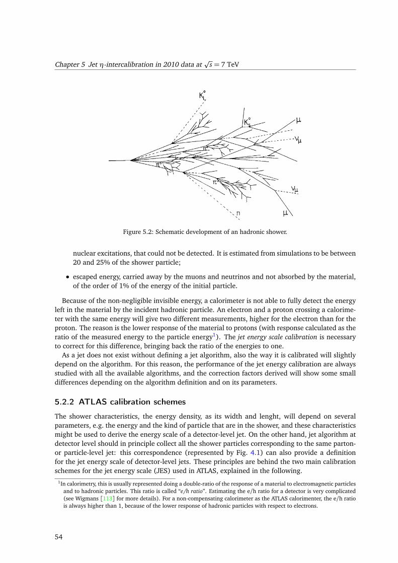
Chapter 5 Jet η-intercalibration in 2010 data atp
s = 7 TeV
Figure 5.2: Schematic development of an hadronic shower.
nuclear excitations, that could not be detected. It is estimated from simulations to be between20 and 25% of the shower particle;
• escaped energy, carried away by the muons and neutrinos and not absorbed by the material,of the order of 1% of the energy of the initial particle.
Because of the non-negligible invisible energy, a calorimeter is not able to fully detect the energyleft in the material by the incident hadronic particle. An electron and a proton crossing a calorime-ter with the same energy will give two different measurements, higher for the electron than for theproton. The reason is the lower response of the material to protons (with response calculated as theratio of the measured energy to the particle energy1). The jet energy scale calibration is necessaryto correct for this difference, bringing back the ratio of the energies to one.
As a jet does not exist without defining a jet algorithm, also the way it is calibrated will slightlydepend on the algorithm. For this reason, the performance of the jet energy calibration are alwaysstudied with all the available algorithms, and the correction factors derived will show some smalldifferences depending on the algorithm definition and on its parameters.
5.2.2 ATLAS calibration schemes
The shower characteristics, the energy density, as its width and lenght, will depend on severalparameters, e.g. the energy and the kind of particle that are in the shower, and these characteristicsmight be used to derive the energy scale of a detector-level jet. On the other hand, jet algorithm atdetector level should in principle collect all the shower particles corresponding to the same parton-or particle-level jet: this correspondence (represented by Fig. 4.1) can also provide a definitionfor the jet energy scale of detector-level jets. These principles are behind the two main calibrationschemes for the jet energy scale (JES) used in ATLAS, explained in the following.
1In calorimetry, this is usually represented doing a double-ratio of the response of a material to electromagnetic particlesand to hadronic particles. This ratio is called “e/h ratio”. Estimating the e/h ratio for a detector is very complicated(see Wigmans [113] for more details). For a non-compensating calorimeter as the ATLAS calorimenter, the e/h ratiois always higher than 1, because of the lower response of hadronic particles with respect to electrons.
54
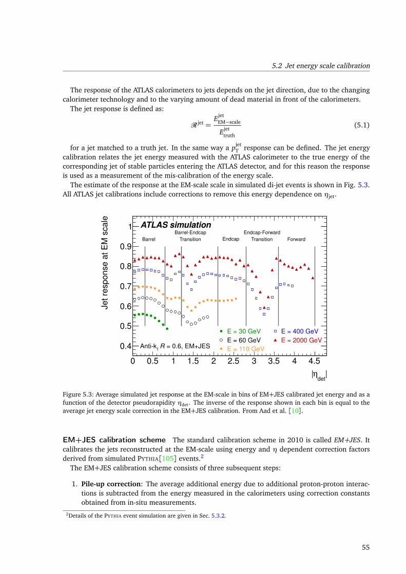
5.2 Jet energy scale calibration
The response of the ATLAS calorimeters to jets depends on the jet direction, due to the changingcalorimeter technology and to the varying amount of dead material in front of the calorimeters.
The jet response is defined as:
R jet =Ejet
EM−scale
Ejettruth
(5.1)
for a jet matched to a truth jet. In the same way a pjetT response can be defined. The jet energy
calibration relates the jet energy measured with the ATLAS calorimeter to the true energy of thecorresponding jet of stable particles entering the ATLAS detector, and for this reason the responseis used as a measurement of the mis-calibration of the energy scale.
The estimate of the response at the EM-scale scale in simulated di-jet events is shown in Fig. 5.3.All ATLAS jet calibrations include corrections to remove this energy dependence on ηjet.
|det
η|
0 0.5 1 1.5 2 2.5 3 3.5 4 4.5
Je
t re
sp
on
se
at
EM
sca
le
0.4
0.5
0.6
0.7
0.8
0.9
1
E = 30 GeV
E = 60 GeV
E = 110 GeV
E = 400 GeV
E = 2000 GeV
Forward
EndcapForward
TransitionEndcap
BarrelEndcap
TransitionBarrel
= 0.6, EM+JESR t
Antik
ATLAS simulation
Figure 5.3: Average simulated jet response at the EM-scale in bins of EM+JES calibrated jet energy and as afunction of the detector pseudorapidity ηdet. The inverse of the response shown in each bin is equal to theaverage jet energy scale correction in the EM+JES calibration. From Aad et al. [10].
EM+JES calibration scheme The standard calibration scheme in 2010 is called EM+JES. Itcalibrates the jets reconstructed at the EM-scale using energy and η dependent correction factorsderived from simulated PYTHIA[105] events.2
The EM+JES calibration scheme consists of three subsequent steps:
1. Pile-up correction: The average additional energy due to additional proton-proton interac-tions is subtracted from the energy measured in the calorimeters using correction constantsobtained from in-situ measurements.
2Details of the PYTHIA event simulation are given in Sec. 5.3.2.
55
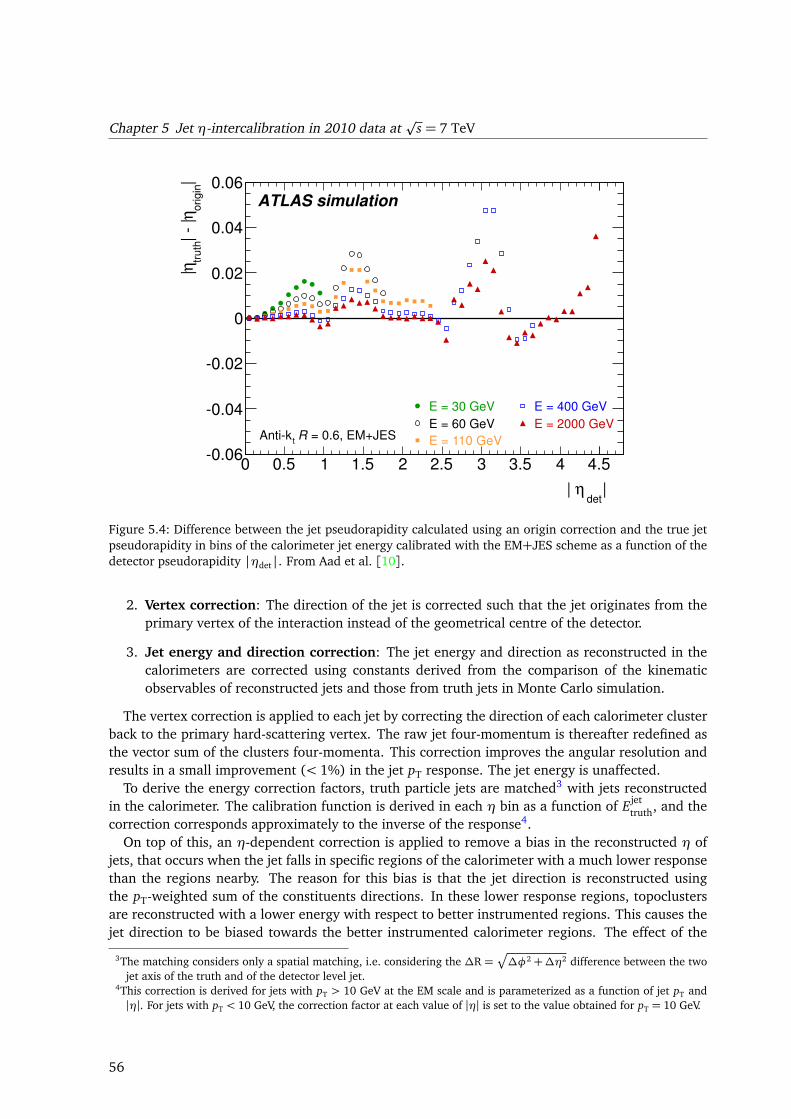
Chapter 5 Jet η-intercalibration in 2010 data atp
s = 7 TeV
|det
η|
0 0.5 1 1.5 2 2.5 3 3.5 4 4.5
|origin
η|
|tr
uth
η|
0.06
0.04
0.02
0
0.02
0.04
0.06
E = 30 GeV
E = 60 GeV
E = 110 GeV
E = 400 GeV
E = 2000 GeV = 0.6, EM+JESR
tAntik
ATLAS simulation
Figure 5.4: Difference between the jet pseudorapidity calculated using an origin correction and the true jetpseudorapidity in bins of the calorimeter jet energy calibrated with the EM+JES scheme as a function of thedetector pseudorapidity |ηdet|. From Aad et al. [10].
2. Vertex correction: The direction of the jet is corrected such that the jet originates from theprimary vertex of the interaction instead of the geometrical centre of the detector.
3. Jet energy and direction correction: The jet energy and direction as reconstructed in thecalorimeters are corrected using constants derived from the comparison of the kinematicobservables of reconstructed jets and those from truth jets in Monte Carlo simulation.
The vertex correction is applied to each jet by correcting the direction of each calorimeter clusterback to the primary hard-scattering vertex. The raw jet four-momentum is thereafter redefined asthe vector sum of the clusters four-momenta. This correction improves the angular resolution andresults in a small improvement (< 1%) in the jet pT response. The jet energy is unaffected.
To derive the energy correction factors, truth particle jets are matched3 with jets reconstructedin the calorimeter. The calibration function is derived in each η bin as a function of Ejet
truth, and thecorrection corresponds approximately to the inverse of the response4.
On top of this, an η-dependent correction is applied to remove a bias in the reconstructed η ofjets, that occurs when the jet falls in specific regions of the calorimeter with a much lower responsethan the regions nearby. The reason for this bias is that the jet direction is reconstructed usingthe pT-weighted sum of the constituents directions. In these lower response regions, topoclustersare reconstructed with a lower energy with respect to better instrumented regions. This causes thejet direction to be biased towards the better instrumented calorimeter regions. The effect of the
3The matching considers only a spatial matching, i.e. considering the ∆R =p
∆φ2 +∆η2 difference between the twojet axis of the truth and of the detector level jet.
4This correction is derived for jets with pT > 10 GeV at the EM scale and is parameterized as a function of jet pT and|η|. For jets with pT < 10 GeV, the correction factor at each value of |η| is set to the value obtained for pT = 10 GeV.
56
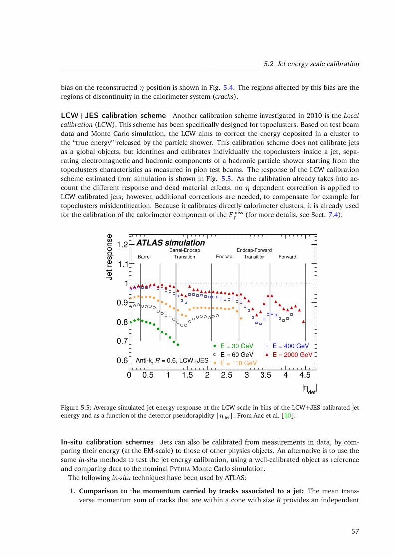
5.2 Jet energy scale calibration
bias on the reconstructed η position is shown in Fig. 5.4. The regions affected by this bias are theregions of discontinuity in the calorimeter system (cracks).
LCW+JES calibration scheme Another calibration scheme investigated in 2010 is the Localcalibration (LCW). This scheme has been specifically designed for topoclusters. Based on test beamdata and Monte Carlo simulation, the LCW aims to correct the energy deposited in a cluster tothe “true energy” released by the particle shower. This calibration scheme does not calibrate jetsas a global objects, but identifies and calibrates individually the topoclusters inside a jet, sepa-rating electromagnetic and hadronic components of a hadronic particle shower starting from thetopoclusters characteristics as measured in pion test beams. The response of the LCW calibrationscheme estimated from simulation is shown in Fig. 5.5. As the calibration already takes into ac-count the different response and dead material effects, no η dependent correction is applied toLCW calibrated jets; however, additional corrections are needed, to compensate for example fortopoclusters misidentification. Because it calibrates directly calorimeter clusters, it is already usedfor the calibration of the calorimeter component of the Emiss
T (for more details, see Sect. 7.4).
|det
η|
0 0.5 1 1.5 2 2.5 3 3.5 4 4.5
Je
t re
sp
on
se
0.6
0.7
0.8
0.9
1
1.1
1.2
E = 30 GeV
E = 60 GeV
E = 110 GeV
E = 400 GeV
E = 2000 GeV
Forward
EndcapForward
TransitionEndcap
BarrelEndcap
TransitionBarrel
= 0.6, LCW+JESR t
Antik
ATLAS simulation
Figure 5.5: Average simulated jet energy response at the LCW scale in bins of the LCW+JES calibrated jetenergy and as a function of the detector pseudorapidity |ηdet|. From Aad et al. [10].
In-situ calibration schemes Jets can also be calibrated from measurements in data, by com-paring their energy (at the EM-scale) to those of other physics objects. An alternative is to use thesame in-situ methods to test the jet energy calibration, using a well-calibrated object as referenceand comparing data to the nominal PYTHIA Monte Carlo simulation.
The following in-situ techniques have been used by ATLAS:
1. Comparison to the momentum carried by tracks associated to a jet: The mean trans-verse momentum sum of tracks that are within a cone with size R provides an independent
57
Chapter 5 Jet η-intercalibration in 2010 data atp
s = 7 TeV
test of the calorimeter energy scale over the entire measured pjetT range within the tracking
acceptance. The comparison is done in the jet ηjet range 0≤ |η|< 2.1.
2. Direct pT balance between a photon and a jet: Events with a photon and one jet at hightransverse momentum are used to compare the transverse momentum of the jet to that ofthe photon. To account for effects like soft QCD radiation and energy migrating out of the jetarea the data are compared to the Monte Carlo simulation. The comparison is done in the jetη range 1.2 and for photon transverse momenta 25≤ pγT < 250 GeV.
3. Photon pT balance to hadronic recoil: The photon transverse momentum is balancedagainst the full hadronic recoil using the projection of the missing transverse momentumonto the photon direction (MPF). This method does not explicitly involve a jet algorithm.The comparison is done in the same kinematic region as the direct photon balance method.
4. Balance between a high-pT jet and low-pT jet system: If jets at low transverse momentumare well-calibrated, jets at high transverse momentum can be balanced against a recoil systemof low transverse momentum jets. This method can probe the jet energy scale up to the TeV-regime. The η range used for the comparison is 2.8.
5. η-intercalibration: The relative jet calorimeter response is studied by comparing the trans-verse momenta of a well-calibrated central jet and a jet in the forward region in events withonly two jets at high transverse momenta (dijets).
All methods are applied to data and Monte Carlo simulation.These in-situ techniques usually rely on assumptions that are only approximately fulfilled. An
example is the assumption that the jet to be calibrated and the reference object are balanced intransverse momentum. This balance can be altered by the presence of additional high-pT particles.For the determination of the JES uncertainties the modelling of physics effects has to be disen-tangled from detector effects.
In 2010 the in-situ techniques have been used to validate the systematic uncertainty in the jetenergy measurement. The η-intercalibration, because of its characteristics, is instead used to es-timate the systematic uncertainty of the forward region with respect to the central region, and forthis reason is very important for 2010 analyses using the full calorimeter coverage.
In order to be used as calibration techniques, a larger integrated luminosity is needed. Thisoption has been used in 2011 for the first time. Some comments on this will be given in Sect. 5.4.
5.3 In-situ η-intercalibration of the ATLAS detector usingdi-jet events
5.3.1 Methods used in this analysis
The η-intercalibration is a “tag-and-probe” analysis using di-jet events. A true di-jet event consistsof two jets that are balanced in pjet
T and 180 apart from each other in the transverse plane, becauseof transverse momentum conservation. Such an event, reconstructed in a detector, could eventuallyshow a difference in the two pjet
T . The pjetT imbalance could occur because of the different energy
response and resolution of the different regions of the calorimeter. For this reason, we expect theeffect to be dependent on ηdet (detector pseudo-rapidity) and pjet
T .
58
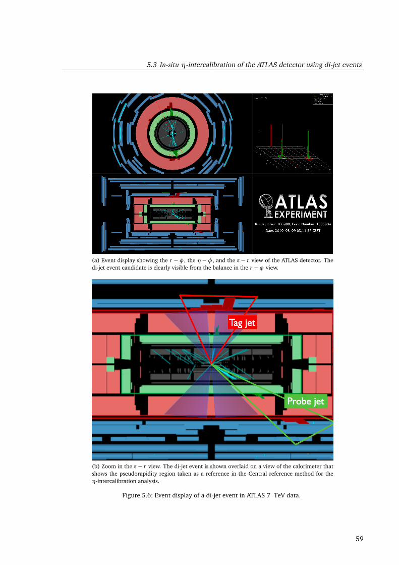
5.3 In-situ η-intercalibration of the ATLAS detector using di-jet events
(a) Event display showing the r −φ, the η−φ, and the z − r view of the ATLAS detector. Thedi-jet event candidate is clearly visible from the balance in the r −φ view.
(b) Zoom in the z − r view. The di-jet event is shown overlaid on a view of the calorimeter thatshows the pseudorapidity region taken as a reference in the Central reference method for theη-intercalibration analysis.
Figure 5.6: Event display of a di-jet event in ATLAS 7 TeV data.
59
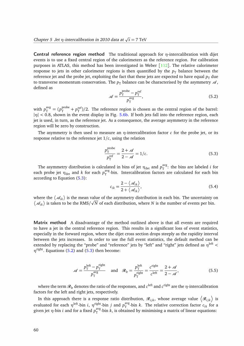
Chapter 5 Jet η-intercalibration in 2010 data atp
s = 7 TeV
Central reference region method The traditional approach for η-intercalibration with dijetevents is to use a fixed central region of the calorimeters as the reference region. For calibrationpurposes in ATLAS, this method has been investigated in Weber [112]. The relative calorimeterresponse to jets in other calorimeter regions is then quantified by the pT balance between thereference jet and the probe jet, exploiting the fact that these jets are expected to have equal pT dueto transverse momentum conservation. The pT balance can be characterised by the asymmetryA ,defined as
A =pprobe
T − prefT
pavgT
, (5.2)
with pavgT = (pprobe
T + prefT )/2. The reference region is chosen as the central region of the barrel:
|η| < 0.8, shown in the event display in Fig. 5.6b. If both jets fall into the reference region, eachjet is used, in turn, as the reference jet. As a consequence, the average asymmetry in the referenceregion will be zero by construction.
The asymmetry is then used to measure an η-intercalibration factor c for the probe jet, or itsresponse relative to the reference jet 1/c, using the relation
pprobeT
prefT
=2+A2−A
= 1/c. (5.3)
The asymmetry distribution is calculated in bins of jet ηdet and pavgT : the bins are labeled i for
each probe jet ηdet and k for each pavgT -bin. Intercalibration factors are calculated for each bin
according to Equation (5.3):
cik =2−
Aik
2+
Aik , (5.4)
where the
Aik
is the mean value of the asymmetry distribution in each bin. The uncertainty on
Aik
is taken to be the RMS/p
N of each distribution, where N is the number of events per bin.
Matrix method A disadvantage of the method outlined above is that all events are requiredto have a jet in the central reference region. This results in a significant loss of event statistics,especially in the forward region, where the dijet cross section drops steeply as the rapidity intervalbetween the jets increases. In order to use the full event statistics, the default method can beextended by replacing the “probe” and “reference” jets by “left” and “right” jets defined as ηleft <
ηright. Equations (5.2) and (5.3) then become:
A =pleft
T − prightT
pavgT
and Rlr =pleft
T
prightT
=cright
cleft=
2+A2−A
, (5.5)
where the termRlr denotes the ratio of the responses, and cleft and cright are the η-intercalibrationfactors for the left and right jets, respectively.
In this approach there is a response ratio distribution, Ri jk, whose average value¬
Ri jk
¶
isevaluated for each ηleft-bin i, ηright-bin j and pavg
T -bin k. The relative correction factor cik for agiven jet η-bin i and for a fixed pavg
T -bin k, is obtained by minimising a matrix of linear equations:
60
5.3 In-situ η-intercalibration of the ATLAS detector using di-jet events
S(c1k, ..., cNk) =N∑
j=1
j−1∑
i=1
1
∆¬
Ri jk
¶
cik
¬
Ri jk
¶
− c jk
!2
+ X (cik), (5.6)
where N denotes the number of η-bins, ∆¬
Ri jk
¶
is the statistical uncertainty of¬
Ri jk
¶
andthe function X (cik) is used to avoid the trivial solution5. Note that if the jet response does notvary with ηjet, then the relative response will be unity for each (ηleft,ηright)-bin combination (seeEquation 5.5). A perfect minimization S = 0 is achieved when all correction factors equal unity.
The minimisation of Equation 5.6 is done separately for each pavgT -bin k, and the resulting cal-
ibration factors cik (for each jet η-bin i) are scaled such that the average calibration factor in thereference region |η|< 0.8 equals unity.
The advantages and disadvantages of the two methods are summarized in Table 5.1.
Method Central reference method Matrix method
type calibration wrt “reference region” calibration factors obtained via
(usually: inside barrel) minimization of matrix of lin. eqs.,
rescale barrel to 1 for comparison
tag jet in reference region (=tag jet) from any detector region
probe jet from any detector region from any detector region
pro easy computing and uncertainties high statistics
contra low statistics CPU time (for minimization procedure)
uncertainties
Table 5.1: Comparison between η-intercalibration methods used in 2010.
In early data, both methods have been used, to have an independent cross-check of the results.No disagreement between them was found.
5.3.2 Data and Monte Carlo samples
The data analysed were collected in 2010, and the total amount of data recorded is 38± 4 pb−1.The exact amount of data in the different bins is different and depends on the evolution, in thedifferent data periods, of the triggers used for the selection of events in each bin.
The standard MC samples used for the comparison with data have been generated with PYTHIA
6.4.21 [105]. PYTHIA implements a leading-order matrix element generation for QCD 2 → 2 pro-cesses, followed by fragmentation, calculated in leading-logarithm approximation, and hadronisa-tion, performed using the Lund String model. The underlying event is multiple-parton interactioninterleaved with the initial state parton shower.
5X (cik) = K
N−1bins
∑Nbinsi=1 cik − 1
2is defined with K being a constant and Nbins being the number of η-bins (number of
indices i). This term prevents the minimisation from choosing the trivial solution: all cik equal to zero. The value ofthe constant K does not impact the solution as long as it is sufficiently large (K ≈ 106).
61
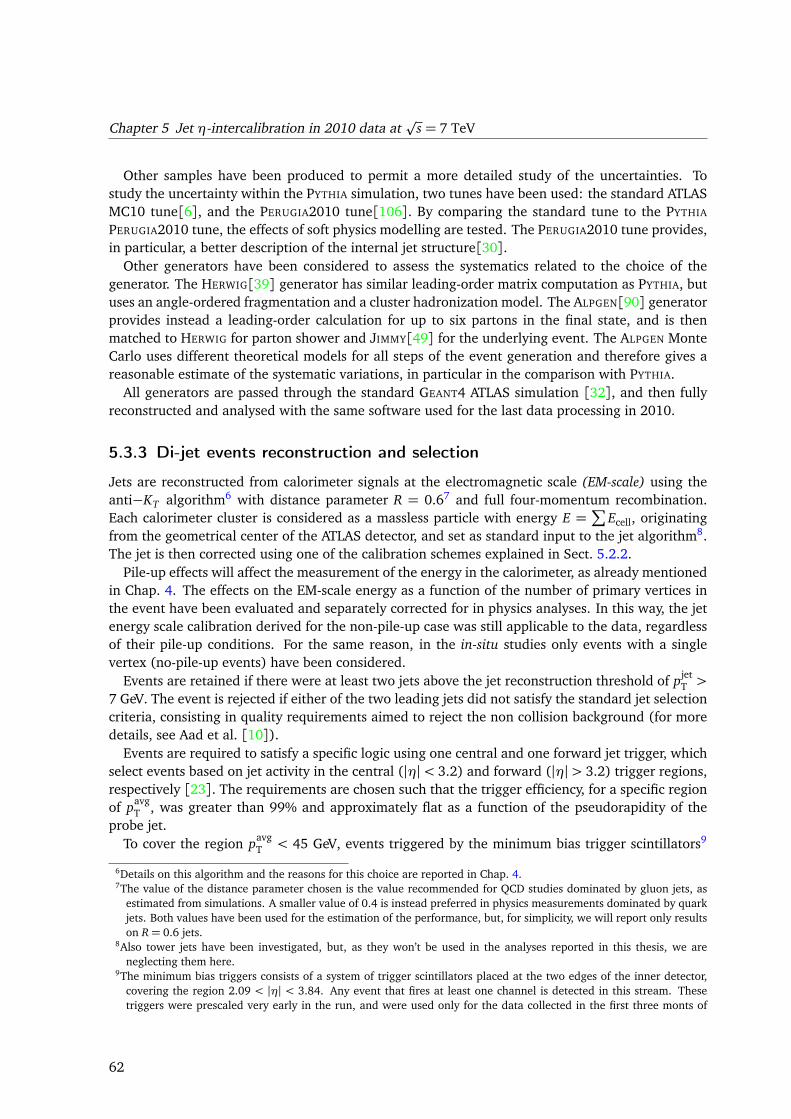
Chapter 5 Jet η-intercalibration in 2010 data atp
s = 7 TeV
Other samples have been produced to permit a more detailed study of the uncertainties. Tostudy the uncertainty within the PYTHIA simulation, two tunes have been used: the standard ATLASMC10 tune[6], and the PERUGIA2010 tune[106]. By comparing the standard tune to the PYTHIA
PERUGIA2010 tune, the effects of soft physics modelling are tested. The PERUGIA2010 tune provides,in particular, a better description of the internal jet structure[30].
Other generators have been considered to assess the systematics related to the choice of thegenerator. The HERWIG[39] generator has similar leading-order matrix computation as PYTHIA, butuses an angle-ordered fragmentation and a cluster hadronization model. The ALPGEN[90] generatorprovides instead a leading-order calculation for up to six partons in the final state, and is thenmatched to HERWIG for parton shower and JIMMY[49] for the underlying event. The ALPGEN MonteCarlo uses different theoretical models for all steps of the event generation and therefore gives areasonable estimate of the systematic variations, in particular in the comparison with PYTHIA.
All generators are passed through the standard GEANT4 ATLAS simulation [32], and then fullyreconstructed and analysed with the same software used for the last data processing in 2010.
5.3.3 Di-jet events reconstruction and selection
Jets are reconstructed from calorimeter signals at the electromagnetic scale (EM-scale) using theanti−KT algorithm6 with distance parameter R = 0.67 and full four-momentum recombination.Each calorimeter cluster is considered as a massless particle with energy E =
∑
Ecell, originatingfrom the geometrical center of the ATLAS detector, and set as standard input to the jet algorithm8.The jet is then corrected using one of the calibration schemes explained in Sect. 5.2.2.
Pile-up effects will affect the measurement of the energy in the calorimeter, as already mentionedin Chap. 4. The effects on the EM-scale energy as a function of the number of primary vertices inthe event have been evaluated and separately corrected for in physics analyses. In this way, the jetenergy scale calibration derived for the non-pile-up case was still applicable to the data, regardlessof their pile-up conditions. For the same reason, in the in-situ studies only events with a singlevertex (no-pile-up events) have been considered.
Events are retained if there were at least two jets above the jet reconstruction threshold of pjetT >
7 GeV. The event is rejected if either of the two leading jets did not satisfy the standard jet selectioncriteria, consisting in quality requirements aimed to reject the non collision background (for moredetails, see Aad et al. [10]).
Events are required to satisfy a specific logic using one central and one forward jet trigger, whichselect events based on jet activity in the central (|η|< 3.2) and forward (|η|> 3.2) trigger regions,respectively [23]. The requirements are chosen such that the trigger efficiency, for a specific regionof pavg
T , was greater than 99% and approximately flat as a function of the pseudorapidity of theprobe jet.
To cover the region pavgT < 45 GeV, events triggered by the minimum bias trigger scintillators9
6Details on this algorithm and the reasons for this choice are reported in Chap. 4.7The value of the distance parameter chosen is the value recommended for QCD studies dominated by gluon jets, as
estimated from simulations. A smaller value of 0.4 is instead preferred in physics measurements dominated by quarkjets. Both values have been used for the estimation of the performance, but, for simplicity, we will report only resultson R= 0.6 jets.
8Also tower jets have been investigated, but, as they won’t be used in the analyses reported in this thesis, we areneglecting them here.
9The minimum bias triggers consists of a system of trigger scintillators placed at the two edges of the inner detector,covering the region 2.09 < |η| < 3.84. Any event that fires at least one channel is detected in this stream. Thesetriggers were prescaled very early in the run, and were used only for the data collected in the first three monts of
62
5.3 In-situ η-intercalibration of the ATLAS detector using di-jet events
were used.To enhance events which have only two jets at high pT, the following selection criteria are ap-
plied;
pavgT > 20 GeV, ∆φ(j1, j2)> 2.6 rad, (5.7)
pT(j3)<max(0.15 pavgT , 7 GeV), (5.8)
where ji denotes the ith highest pT jet in the event and ∆φ(j1, j2) is the azimuthal angle betweenthe two leading jets.
The lowest pavgT -bins are likely to suffer from biases. At very low pavg
T , it is expected that thistechnique may not measure accurately the relative response to jets, because the assumption ofdijet balance at hadron level may start to fail. First, there are residual low-pT jet effects sincethe selection criterion on the third jet, which is used to suppress the unbalancing effects of softQCD radiation, is not as efficient due to the jet reconstruction threshold of 7 GeV. Second, the jetreconstruction efficiency is worse for low-pT jets.
5.3.4 Results
In Fig. 5.7, a comparison between the data and the PYTHIA simulation is shown. The comparisonbetween the particle-level jets (labeled as “Dijet Truth”) and the reconstructed jets (labeled as“Dijet MC”) in the PYTHIA samples shows already the effects expected in the analysis. In general,the relative response is expected to be close to 1 for |η| < 2, with fluctuations mostly located inthe points where the calorimeter structure, and so the response, changes (see Fig. 5.3). At largepseudo-rapidities (|η|> 3, roughly corresponding with the FCal system) both the reconstructed andthe truth jets show a relative response smaller than one: this means that not only the calorimeterresponse, but also a physics effect is playing a role, as will be discussed later in the text.
When compared with the data, the most striking feature is that the data does not follow thesimulation behavior at high |η|. The comparison between Fig. 5.7a and 5.7b shows that thecalibration is not responsible for this discrepancy. The results shown are produced with the centralreference region method and cross-checked with the matrix method; the two methods agree withinthe statistical uncertainties.
To interpret the observations, the comparison has been performed10 with the set of samplesmentioned in 5.3.2. In Fig. 5.8 the behavior of the four systematic samples is overlaid on the data,for four different pavg
T bins. The behavior is different mostly at low pavgT : the PYTHIA samples (both
the standard and the PERUGIA2010 tune) tend to have a lower response than the one seen in data,while the HERWIG sample (and the ALPGEN+HERWIG as well) tend to have a higher response. Thedifference can be of the order of 10% at 20 GeV and large η. The effect has been tested againstcalibration effects, uncertainties on the soft radiation11 and underlying event simulation, and inall cases the results were consistent with the picture given. This result has been interpreted as aneffect of the different parton shower. This could explain the large difference between HERWIG and
operations (2010 run period A, B and C).10In this comparison, due to the lower statistics of the systematic samples, only the matrix method has been used. Also,
the binning in η is slightly coarser, in order to provide a result more robust against statistical fluctuations.11This uncertainty is related to the selection cuts listed in Eqs. 5.8. To assess the uncertainty, the selection criteria
are varied for both data and Monte Carlo. The resulting uncertainty is negligible with respect to the modellinguncertainty.
63
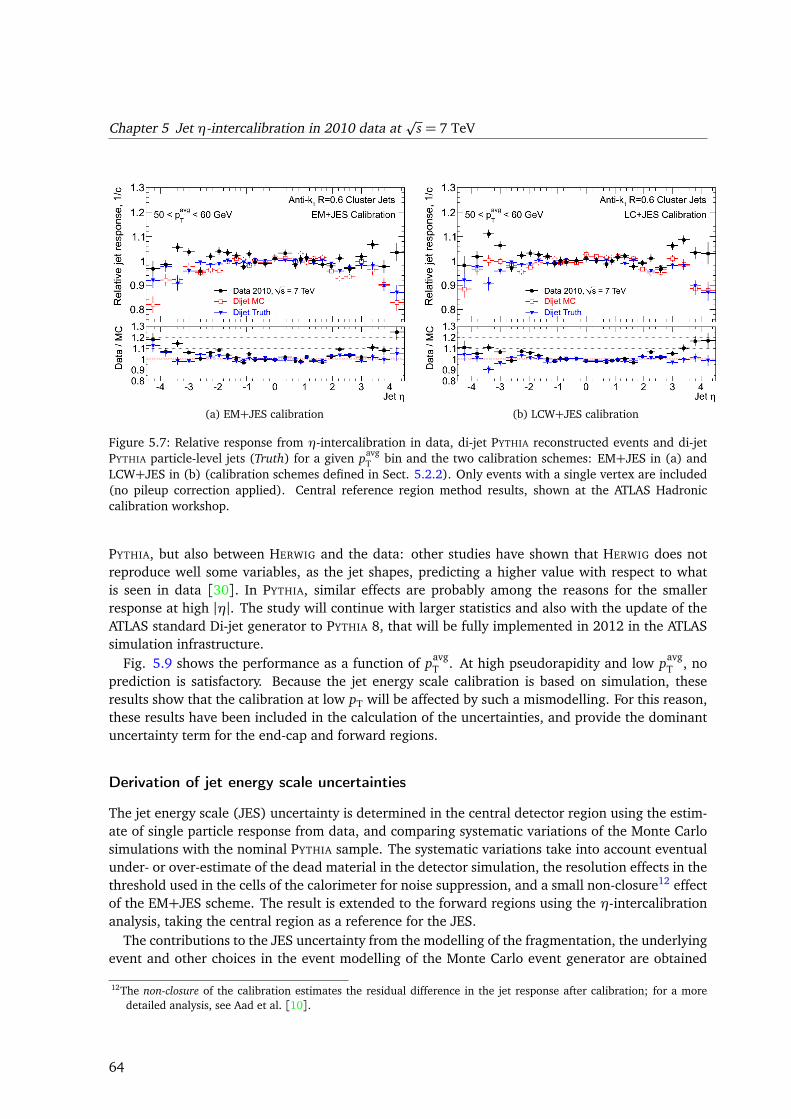
Chapter 5 Jet η-intercalibration in 2010 data atp
s = 7 TeV
(a) EM+JES calibration (b) LCW+JES calibration
Figure 5.7: Relative response from η-intercalibration in data, di-jet PYTHIA reconstructed events and di-jetPYTHIA particle-level jets (Truth) for a given pavg
T bin and the two calibration schemes: EM+JES in (a) andLCW+JES in (b) (calibration schemes defined in Sect. 5.2.2). Only events with a single vertex are included(no pileup correction applied). Central reference region method results, shown at the ATLAS Hadroniccalibration workshop.
PYTHIA, but also between HERWIG and the data: other studies have shown that HERWIG does notreproduce well some variables, as the jet shapes, predicting a higher value with respect to whatis seen in data [30]. In PYTHIA, similar effects are probably among the reasons for the smallerresponse at high |η|. The study will continue with larger statistics and also with the update of theATLAS standard Di-jet generator to PYTHIA 8, that will be fully implemented in 2012 in the ATLASsimulation infrastructure.
Fig. 5.9 shows the performance as a function of pavgT . At high pseudorapidity and low pavg
T , noprediction is satisfactory. Because the jet energy scale calibration is based on simulation, theseresults show that the calibration at low pT will be affected by such a mismodelling. For this reason,these results have been included in the calculation of the uncertainties, and provide the dominantuncertainty term for the end-cap and forward regions.
Derivation of jet energy scale uncertainties
The jet energy scale (JES) uncertainty is determined in the central detector region using the estim-ate of single particle response from data, and comparing systematic variations of the Monte Carlosimulations with the nominal PYTHIA sample. The systematic variations take into account eventualunder- or over-estimate of the dead material in the detector simulation, the resolution effects in thethreshold used in the cells of the calorimeter for noise suppression, and a small non-closure12 effectof the EM+JES scheme. The result is extended to the forward regions using the η-intercalibrationanalysis, taking the central region as a reference for the JES.
The contributions to the JES uncertainty from the modelling of the fragmentation, the underlyingevent and other choices in the event modelling of the Monte Carlo event generator are obtained
12The non-closure of the calibration estimates the residual difference in the jet response after calibration; for a moredetailed analysis, see Aad et al. [10].
64
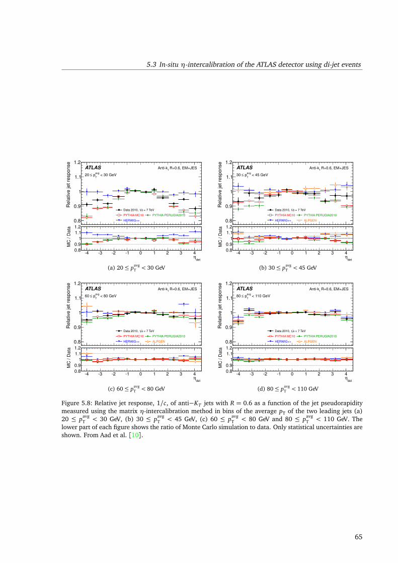
5.3 In-situ η-intercalibration of the ATLAS detector using di-jet eventsR
ela
tive
je
t re
sp
on
se
0.8
0.9
1
1.1
1.2
= 7 TeVsData 2010,
PYTHIA MC10
HERWIG++
PYTHIA PERUGIA2010
ATLAS
< 30 GeVavg
T p≤20
R=0.6, EM+JESt
Antik
detη
4 3 2 1 0 1 2 3 4
MC
/ D
ata
0.8
0.9
1
1.1
1.2
(a) 20≤ pavgT < 30 GeV
Re
lative
je
t re
sp
on
se
0.8
0.9
1
1.1
1.2
= 7 TeVsData 2010,
PYTHIA MC10
HERWIG++ ALPGEN
PYTHIA PERUGIA2010
ATLAS
< 45 GeVavg
T p≤30
R=0.6, EM+JESt
Antik
detη
4 3 2 1 0 1 2 3 4
MC
/ D
ata
0.8
0.9
1
1.1
1.2
(b) 30≤ pavgT < 45 GeV
Re
lative
je
t re
sp
on
se
0.8
0.9
1
1.1
1.2
= 7 TeVsData 2010,
PYTHIA MC10
HERWIG++ ALPGEN
PYTHIA PERUGIA2010
ATLAS
< 80 GeVavg
T p≤60
R=0.6, EM+JESt
Antik
detη
4 3 2 1 0 1 2 3 4
MC
/ D
ata
0.8
0.9
1
1.1
1.2
(c) 60≤ pavgT < 80 GeV
Re
lative
je
t re
sp
on
se
0.8
0.9
1
1.1
1.2
= 7 TeVsData 2010,
PYTHIA MC10
HERWIG++ ALPGEN
PYTHIA PERUGIA2010
ATLAS
< 110 GeVavg
T p≤80
R=0.6, EM+JESt
Antik
detη
4 3 2 1 0 1 2 3 4
MC
/ D
ata
0.8
0.9
1
1.1
1.2
(d) 80≤ pavgT < 110 GeV
Figure 5.8: Relative jet response, 1/c, of anti−KT jets with R = 0.6 as a function of the jet pseudorapiditymeasured using the matrix η-intercalibration method in bins of the average pT of the two leading jets (a)20 ≤ pavg
T < 30 GeV, (b) 30 ≤ pavgT < 45 GeV, (c) 60 ≤ pavg
T < 80 GeV and 80 ≤ pavgT < 110 GeV. The
lower part of each figure shows the ratio of Monte Carlo simulation to data. Only statistical uncertainties areshown. From Aad et al. [10].
65
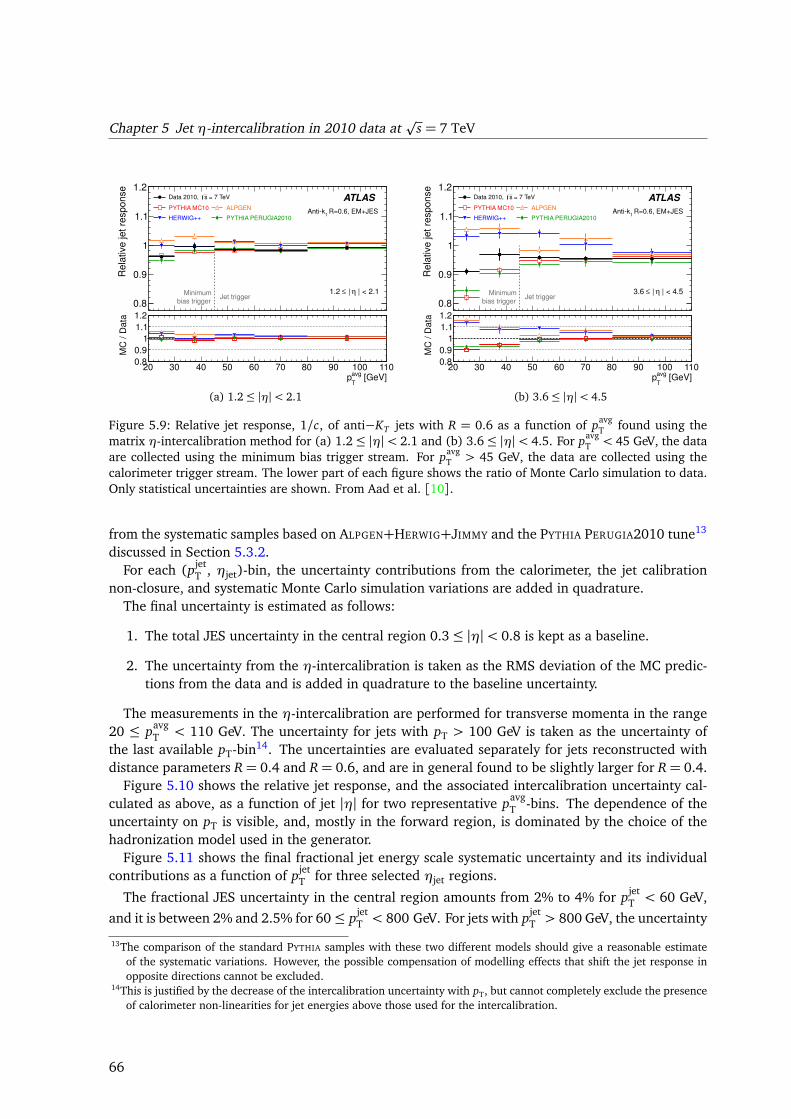
Chapter 5 Jet η-intercalibration in 2010 data atp
s = 7 TeVR
ela
tive
je
t re
sp
on
se
0.8
0.9
1
1.1
1.2 = 7 TeVsData 2010,
PYTHIA MC10
HERWIG++
ALPGEN
PYTHIA PERUGIA2010
| < 2.1η | ≤1.2
ATLAS
Jet triggerMinimum
bias trigger
R=0.6, EM+JESt
Antik
[GeV]avg
Tp
20 30 40 50 60 70 80 90 100 110
MC
/ D
ata
0.8
0.9
1
1.1
1.2
(a) 1.2≤ |η|< 2.1
Re
lative
je
t re
sp
on
se
0.8
0.9
1
1.1
1.2 = 7 TeVsData 2010,
PYTHIA MC10
HERWIG++
ALPGEN
PYTHIA PERUGIA2010
| < 4.5η | ≤3.6
ATLAS
Jet triggerMinimum
bias trigger
R=0.6, EM+JESt
Antik
[GeV]avg
Tp
20 30 40 50 60 70 80 90 100 110
MC
/ D
ata
0.8
0.9
1
1.1
1.2
(b) 3.6≤ |η|< 4.5
Figure 5.9: Relative jet response, 1/c, of anti−KT jets with R = 0.6 as a function of pavgT found using the
matrix η-intercalibration method for (a) 1.2≤ |η|< 2.1 and (b) 3.6≤ |η|< 4.5. For pavgT < 45 GeV, the data
are collected using the minimum bias trigger stream. For pavgT > 45 GeV, the data are collected using the
calorimeter trigger stream. The lower part of each figure shows the ratio of Monte Carlo simulation to data.Only statistical uncertainties are shown. From Aad et al. [10].
from the systematic samples based on ALPGEN+HERWIG+JIMMY and the PYTHIA PERUGIA2010 tune13
discussed in Section 5.3.2.For each (pjet
T , ηjet)-bin, the uncertainty contributions from the calorimeter, the jet calibrationnon-closure, and systematic Monte Carlo simulation variations are added in quadrature.
The final uncertainty is estimated as follows:
1. The total JES uncertainty in the central region 0.3≤ |η|< 0.8 is kept as a baseline.
2. The uncertainty from the η-intercalibration is taken as the RMS deviation of the MC predic-tions from the data and is added in quadrature to the baseline uncertainty.
The measurements in the η-intercalibration are performed for transverse momenta in the range20 ≤ pavg
T < 110 GeV. The uncertainty for jets with pT > 100 GeV is taken as the uncertainty ofthe last available pT-bin14. The uncertainties are evaluated separately for jets reconstructed withdistance parameters R= 0.4 and R= 0.6, and are in general found to be slightly larger for R= 0.4.
Figure 5.10 shows the relative jet response, and the associated intercalibration uncertainty cal-culated as above, as a function of jet |η| for two representative pavg
T -bins. The dependence of theuncertainty on pT is visible, and, mostly in the forward region, is dominated by the choice of thehadronization model used in the generator.
Figure 5.11 shows the final fractional jet energy scale systematic uncertainty and its individualcontributions as a function of pjet
T for three selected ηjet regions.
The fractional JES uncertainty in the central region amounts from 2% to 4% for pjetT < 60 GeV,
and it is between 2% and 2.5% for 60≤ pjetT < 800 GeV. For jets with pjet
T > 800 GeV, the uncertainty
13The comparison of the standard PYTHIA samples with these two different models should give a reasonable estimateof the systematic variations. However, the possible compensation of modelling effects that shift the jet response inopposite directions cannot be excluded.
14This is justified by the decrease of the intercalibration uncertainty with pT, but cannot completely exclude the presenceof calorimeter non-linearities for jet energies above those used for the intercalibration.
66
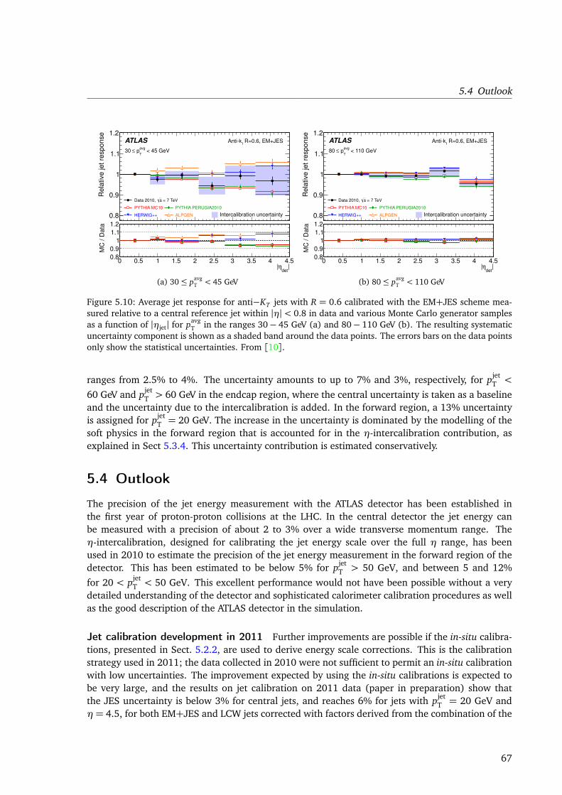
5.4 OutlookR
ela
tive
je
t re
sp
on
se
0.8
0.9
1
1.1
1.2
= 7 TeVsData 2010,
PYTHIA MC10
HERWIG++ ALPGEN
PYTHIA PERUGIA2010
Intercalibration uncertainty
ATLAS
< 45 GeVavg
T p≤30
R=0.6, EM+JESt
Antik
|det
η|0 0.5 1 1.5 2 2.5 3 3.5 4 4.5
MC
/ D
ata
0.8
0.9
1
1.1
1.2
(a) 30≤ pavgT < 45 GeV
Re
lative
je
t re
sp
on
se
0.8
0.9
1
1.1
1.2
= 7 TeVsData 2010,
PYTHIA MC10
HERWIG++ ALPGEN
PYTHIA PERUGIA2010
Intercalibration uncertainty
ATLAS
< 110 GeVavg
T p≤80
R=0.6, EM+JESt
Antik
|det
η|0 0.5 1 1.5 2 2.5 3 3.5 4 4.5
MC
/ D
ata
0.8
0.9
1
1.1
1.2
(b) 80≤ pavgT < 110 GeV
Figure 5.10: Average jet response for anti−KT jets with R = 0.6 calibrated with the EM+JES scheme mea-sured relative to a central reference jet within |η| < 0.8 in data and various Monte Carlo generator samplesas a function of |ηjet| for pavg
T in the ranges 30− 45 GeV (a) and 80− 110 GeV (b). The resulting systematicuncertainty component is shown as a shaded band around the data points. The errors bars on the data pointsonly show the statistical uncertainties. From [10].
ranges from 2.5% to 4%. The uncertainty amounts to up to 7% and 3%, respectively, for pjetT <
60 GeV and pjetT > 60 GeV in the endcap region, where the central uncertainty is taken as a baseline
and the uncertainty due to the intercalibration is added. In the forward region, a 13% uncertaintyis assigned for pjet
T = 20 GeV. The increase in the uncertainty is dominated by the modelling of thesoft physics in the forward region that is accounted for in the η-intercalibration contribution, asexplained in Sect 5.3.4. This uncertainty contribution is estimated conservatively.
5.4 Outlook
The precision of the jet energy measurement with the ATLAS detector has been established inthe first year of proton-proton collisions at the LHC. In the central detector the jet energy canbe measured with a precision of about 2 to 3% over a wide transverse momentum range. Theη-intercalibration, designed for calibrating the jet energy scale over the full η range, has beenused in 2010 to estimate the precision of the jet energy measurement in the forward region of thedetector. This has been estimated to be below 5% for pjet
T > 50 GeV, and between 5 and 12%
for 20 < pjetT < 50 GeV. This excellent performance would not have been possible without a very
detailed understanding of the detector and sophisticated calorimeter calibration procedures as wellas the good description of the ATLAS detector in the simulation.
Jet calibration development in 2011 Further improvements are possible if the in-situ calibra-tions, presented in Sect. 5.2.2, are used to derive energy scale corrections. This is the calibrationstrategy used in 2011; the data collected in 2010 were not sufficient to permit an in-situ calibrationwith low uncertainties. The improvement expected by using the in-situ calibrations is expected tobe very large, and the results on jet calibration on 2011 data (paper in preparation) show thatthe JES uncertainty is below 3% for central jets, and reaches 6% for jets with pjet
T = 20 GeV andη= 4.5, for both EM+JES and LCW jets corrected with factors derived from the combination of the
67
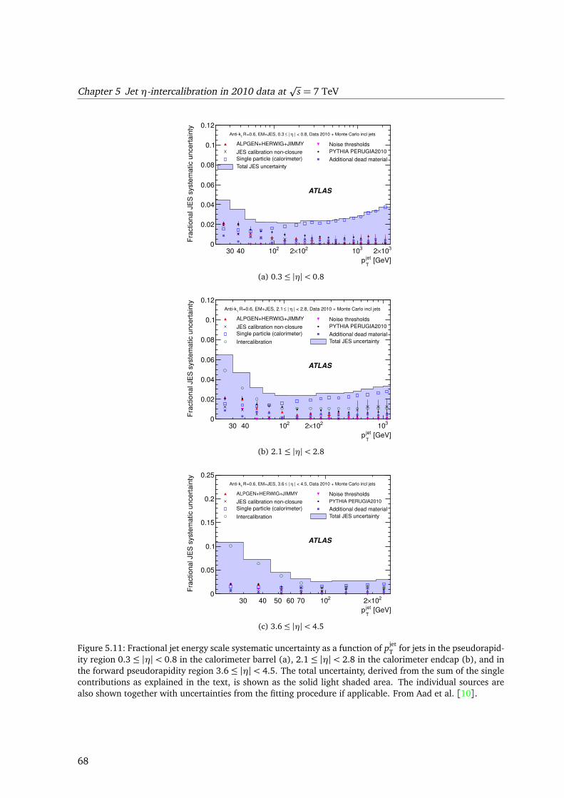
Chapter 5 Jet η-intercalibration in 2010 data atp
s = 7 TeV
[GeV]jet
Tp
30 40 210 210×23
103
10×2
Fra
ctio
na
l JE
S s
yste
ma
tic u
nce
rta
inty
0
0.02
0.04
0.06
0.08
0.1
0.12
ATLAS
| < 0.8, Data 2010 + Monte Carlo incl jetsη | ≤=0.6, EM+JES, 0.3 R t
Antik
ALPGEN+HERWIG+JIMMY Noise thresholds
JES calibration nonclosure PYTHIA PERUGIA2010
Single particle (calorimeter) Additional dead material
Total JES uncertainty
(a) 0.3≤ |η|< 0.8
[GeV]jet
Tp
30 40 210 210×23
10
Fra
ctio
na
l JE
S s
yste
ma
tic u
nce
rta
inty
0
0.02
0.04
0.06
0.08
0.1
0.12
ATLAS
| < 2.8, Data 2010 + Monte Carlo incl jetsη | ≤=0.6, EM+JES, 2.1 R t
Antik
ALPGEN+HERWIG+JIMMY Noise thresholds
JES calibration nonclosure PYTHIA PERUGIA2010
Single particle (calorimeter) Additional dead material
Intercalibration Total JES uncertainty
(b) 2.1≤ |η|< 2.8
[GeV]jet
Tp
30 40 50 60 70 210 210×2
Fra
ctio
na
l JE
S s
yste
ma
tic u
nce
rta
inty
0
0.05
0.1
0.15
0.2
0.25
ATLAS
| < 4.5, Data 2010 + Monte Carlo incl jetsη | ≤=0.6, EM+JES, 3.6 R t
Antik
ALPGEN+HERWIG+JIMMY Noise thresholds
JES calibration nonclosure PYTHIA PERUGIA2010
Single particle (calorimeter) Additional dead material
Intercalibration Total JES uncertainty
(c) 3.6≤ |η|< 4.5
Figure 5.11: Fractional jet energy scale systematic uncertainty as a function of pjetT for jets in the pseudorapid-
ity region 0.3≤ |η|< 0.8 in the calorimeter barrel (a), 2.1≤ |η|< 2.8 in the calorimeter endcap (b), and inthe forward pseudorapidity region 3.6≤ |η|< 4.5. The total uncertainty, derived from the sum of the singlecontributions as explained in the text, is shown as the solid light shaded area. The individual sources arealso shown together with uncertainties from the fitting procedure if applicable. From Aad et al. [10].
68
5.4 Outlook
different in-situ calibrations. The improvement in the overall uncertainty is about a factor 2 withrespect to 2010 uncertainties.
In the 2011 calibration the η-intercalibration has been used to derive calibration factors to ex-tend the central (|η| < 1.2) JES to the forward region. These factors, and their relative uncer-tainties, have been produced with the matrix method, while the central reference region methodhas provided a cross-check of the results. The matrix method has been preferred for calibrationpurposes to the central reference region method, because it needs lower statistics to calibrate alarge phase-space region. Instead, the central reference region method is used as a baseline forthe measurement of the jet energy resolution in-situ, where a clearly defined reference region isneeded.
2012 goal: 1% jet energy scale uncertainty The JES uncertainty is among the dominantuncertainties in physics analyses in ATLAS. Lowering further this uncertainty is the long term goalof the ATLAS effort; the goal would be to reach the 1% level in 2012. This is a challenging goal,and the main reasons are: the impact of the higher pile-up conditions on the measurement, andthe modelling issues.
In this chapter, I haven’t investigated the pile-up effects on the calibration, as the ATLAS strategyforesees that those effects should be corrected before the calibration is applied. However, in 2010the amount of 1-vertex events was still quite high, and the data and Monte Carlo samples havebeen separated into two subsets: 1-vertex events, where the calibration performance have beenstudies, and events with more than one vertex, where the pile-up effects have been studied, andthe pile-up corrections have been derived. This approach is not feasible when looking at the 2011pile-up conditions (reported in Fig. 3.3); and pile-up can be expected only to increase with higherenergies and luminosities. Every time the bunches conditions will change, a first investigation ofthe calorimeter performance will always be needed, and will be followed by the analysis of theperformance at the jet level. This task is very challenging in particular for the η-intercalibration:pile-up effects will impact the central and forward calorimeters in a different way, and, if notunderstood and corrected properly, might introduce artificial effects in the analysis. The centralreference region method, explained in Sect. 5.3.1, might provide anyway useful inputs, because itpermits to clearly separate the different detector regions in the analysis.
This work has shown how the η-intercalibration can succeed in extending the understandingof the energy scale up to the full calorimeter coverage. The traditional bottle-neck of the in-situcalibrations, i.e. the need of high statistics, has been solved by the matrix method explained in Sect.5.3.1, developed in ATLAS to overcome this difficulty. But the results are still heavily dominatedby the modelling uncertainty. This is related to the difference in the Monte Carlo predictions, andnot at all to the calibration. The only way to solve this issue would be to investigate the generatorsthemselves and find the reason for their difference. As mentioned in Sect. 5.3.4, the parton showeris thought to be responsible for the large uncertainty. A better understanding of PYTHIA and HERWIG
in physics analyses, together with the update of the PYTHIA code to the latest version, foreseen in2012, is expected to shed light on this issue.
69

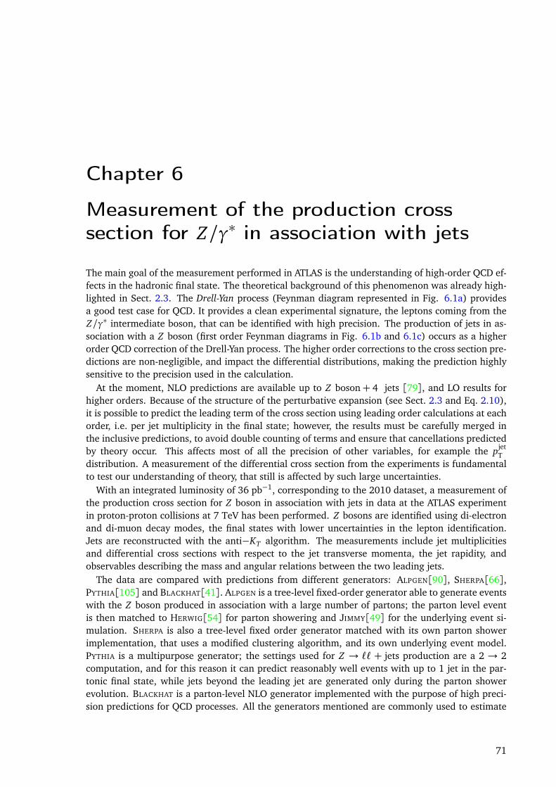
Chapter 6
Measurement of the production crosssection for Z/γ∗ in association with jets
The main goal of the measurement performed in ATLAS is the understanding of high-order QCD ef-fects in the hadronic final state. The theoretical background of this phenomenon was already high-lighted in Sect. 2.3. The Drell-Yan process (Feynman diagram represented in Fig. 6.1a) providesa good test case for QCD. It provides a clean experimental signature, the leptons coming from theZ/γ∗ intermediate boson, that can be identified with high precision. The production of jets in as-sociation with a Z boson (first order Feynman diagrams in Fig. 6.1b and 6.1c) occurs as a higherorder QCD correction of the Drell-Yan process. The higher order corrections to the cross section pre-dictions are non-negligible, and impact the differential distributions, making the prediction highlysensitive to the precision used in the calculation.
At the moment, NLO predictions are available up to Z boson+ 4 jets [79], and LO results forhigher orders. Because of the structure of the perturbative expansion (see Sect. 2.3 and Eq. 2.10),it is possible to predict the leading term of the cross section using leading order calculations at eachorder, i.e. per jet multiplicity in the final state; however, the results must be carefully merged inthe inclusive predictions, to avoid double counting of terms and ensure that cancellations predictedby theory occur. This affects most of all the precision of other variables, for example the pjet
Tdistribution. A measurement of the differential cross section from the experiments is fundamentalto test our understanding of theory, that still is affected by such large uncertainties.
With an integrated luminosity of 36 pb−1, corresponding to the 2010 dataset, a measurement ofthe production cross section for Z boson in association with jets in data at the ATLAS experimentin proton-proton collisions at 7 TeV has been performed. Z bosons are identified using di-electronand di-muon decay modes, the final states with lower uncertainties in the lepton identification.Jets are reconstructed with the anti−KT algorithm. The measurements include jet multiplicitiesand differential cross sections with respect to the jet transverse momenta, the jet rapidity, andobservables describing the mass and angular relations between the two leading jets.
The data are compared with predictions from different generators: ALPGEN[90], SHERPA[66],PYTHIA[105] and BLACKHAT[41]. ALPGEN is a tree-level fixed-order generator able to generate eventswith the Z boson produced in association with a large number of partons; the parton level eventis then matched to HERWIG[54] for parton showering and JIMMY[49] for the underlying event si-mulation. SHERPA is also a tree-level fixed order generator matched with its own parton showerimplementation, that uses a modified clustering algorithm, and its own underlying event model.PYTHIA is a multipurpose generator; the settings used for Z → `` + jets production are a 2 → 2computation, and for this reason it can predict reasonably well events with up to 1 jet in the par-tonic final state, while jets beyond the leading jet are generated only during the parton showerevolution. BLACKHAT is a parton-level NLO generator implemented with the purpose of high preci-sion predictions for QCD processes. All the generators mentioned are commonly used to estimate
71
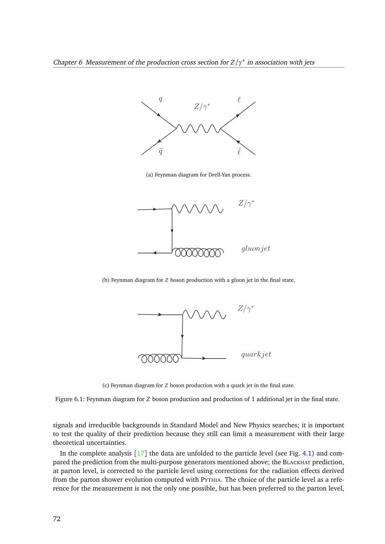
Chapter 6 Measurement of the production cross section for Z/γ∗ in association with jets
q
q
Z/γ∗ ℓ
ℓ
(a) Feynman diagram for Drell-Yan process.
Z/γ∗
gluonjet
(b) Feynman diagram for Z boson production with a gluon jet in the final state.
Z/γ∗
quarkjet
(c) Feynman diagram for Z boson production with a quark jet in the final state.
Figure 6.1: Feynman diagram for Z boson production and production of 1 additional jet in the final state.
signals and irreducible backgrounds in Standard Model and New Physics searches; it is importantto test the quality of their prediction because they still can limit a measurement with their largetheoretical uncertainties.
In the complete analysis [17] the data are unfolded to the particle level (see Fig. 4.1) and com-pared the prediction from the multi-purpose generators mentioned above; the BLACKHAT prediction,at parton level, is corrected to the particle level using corrections for the radiation effects derivedfrom the parton shower evolution computed with PYTHIA. The choice of the particle level as a refe-rence for the measurement is not the only one possible, but has been preferred to the parton level,
72
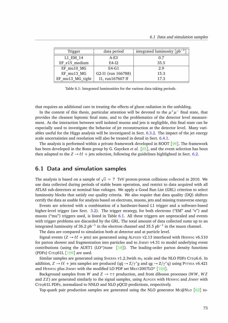
6.1 Data and simulation samples
Trigger data period integrated luminosity [pb−1]
L1_EM_14 A-E3 0.7EF_e15_medium E4-I2 35.5EF_mu10_MG E4-G1 2.9EF_mu13_MG G2-I1 (run 166788) 15.3
EF_mu13_MG_tight I1, run167607 ff 17.3
Table 6.1: Integrated luminosities for the various data taking periods.
that requires an additional care in treating the effects of gluon radiation in the unfolding.In the context of this thesis, particular attention will be devoted to the µ+µ− final state, that
provides the cleanest leptonic final state, and to the problematics of the detector level measure-ment. As the interaction between well isolated muons and jets is negligible, this final state can beexpecially used to investigate the behavior of jet reconstruction at the detector level. Many vari-ables useful for the Higgs analysis will be investigated in Sect. 6.3.2. The impact of the jet energyscale uncertainties and resolution will also be treated in detail in Sect. 6.4.1.
The analysis is performed within a private framework developed in ROOT [99]. The frameworkhas been developed in the Bonn group by G. Gaycken et al. [65], and the event selection has beenthen adapted to the Z → `` + jets selection, following the guidelines highlighted in Sect. 6.2.
6.1 Data and simulation samples
The analysis is based on a sample ofp
s = 7 TeV proton-proton collisions collected in 2010. Weuse data collected during periods of stable beam operation, and restrict to data acquired with allATLAS sub-detectors at nominal bias voltages. We apply a Good Run List (GRL) criterion to selectluminosity blocks that satisfy our quality criteria. We also require that data quality (DQ) shifterscertify the data as usable for analysis based on electrons, muons, jets and missing transverse energy.
Events are selected with a combination of a hardware-based L1 trigger and a software-basedhigher-level trigger (see Sect. 3.2). The trigger strategy, for both electrons (“EM” and “e”) andmuons (“mu”) triggers used, is listed in Table 6.1. All these triggers are unprescaled and eventswith trigger problems are discarded by the GRL. The total amount of data collected sums up to anintegrated luminosity of 36.2 pb−1 in the electron channel and 35.5 pb−1 in the muon channel.
The data are compared to simulation both at detector and at particle level.Signal events (Z → `` + jets) are generated using ALPGEN v2.13 interfaced with HERWIG v6.510
for parton shower and fragmentation into particles and to JIMMY v4.31 to model underlying eventcontributions (using the AUET1 (LO*)tune [18]). The leading-order parton density functions(PDFs) CTEQ61L [109] are used.
Similar samples are generated using SHERPA v1.2.3with mT scale and the NLO PDFs CTEQ6.6. Inaddition, Z → `` + jets samples are produced (qq→ Z/γ∗g and qg→ Z/γ∗q) using PYTHIA v6.421and HERWIG plus JIMMY with the modified LO PDF set MRST2007LO* [104].
Background samples from W and Z → ττ production, and from diboson processes (WW , W Zand Z Z) are generated similarly to the signal samples, using ALPGEN with HERWIG and JIMMY withCTEQ61L PDFs, normalized to NNLO and NLO pQCD predictions, respectively.
Top-quark pair production samples are generated using the NLO generator MC@NLO [63] to-
73
Chapter 6 Measurement of the production cross section for Z/γ∗ in association with jets
gether with the NLO PDF set CTEQ6.6.The generated samples are passed through a full simulation of the ATLAS detector and trigger,
based on GEANT4. The simulated events are then reconstructed and analyzed with the same analysischain as for the data, and the same trigger and event selection criteria. Details of these samples aresummarized in Table 6.2. All samples are part of the ATLAS MC10 production.
The program PHOTOS [68] is used to simulate final state QED radiation in ALPGEN and PYTHIA
samples. SHERPA uses a self designed parton shower algorithm.The W and Z samples are normalized globally to next-to-next-to-leading order (NNLO) pQCD
inclusive Drell-Yan predictions computed by the FEWZ [64] program. For hadron-level comparisons,the PYTHIA Z → `` + jets cross sections are later scaled to the cross section measured in data. Theresulting global scale factor is 1.186± 0.021.
The Pile-up simulation corresponds to a bunch-train setup with double trains with 225 ns (= 9BC) separation, each containing 8 filled bunches with 150 ns bunch separation. The train arrange-ment reproduces the accelerator settings used from Run period D onwards, i.e. in the data usedfor this analysis. The number of minimum-bias interactions follows a Poisson distribution with amean of approximately two. These samples have been re-weighted such that the distributions ofthe primary vertices follows the distribution observed in data. The weights have been derived at anearly preselection stage, to avoid selection biases.
The multi-jets background, instead, is extracted from data. The presence of this background isdue to the mis-identification of a jet as a lepton. In the electron channel, is dominated by jets fakingelectrons in the final state, thus by a calorimeter mis-measurement or by a mis-identification; in themuon channel, mainly originates from heavy-flavour jet production processes, with muons frombottom and charm quark decays, as well as from the decay-in-flight of pions and kaons, which arehighly suppressed by the isolation requirement applied to the muon candidates (see Sect. 6.2). Forthis reason, the influence of this background is higher in the electron channel than in the muonchannel.
6.2 Z → `` + jets selection
The selection requirement for event selection are compatible with all ATLAS analyses. In particular,data quality requirements on the luminosity blocks considered for the analysis are applied beforethe object selection.
Z boson selection
Quality requirements on the leptons are applied, and they are compatible with those applied in theother W and Z boson analyses. Those requirements are treated in detail in [8] for electrons and in[19, 20] for muons. As this chapter will mostly focus on muons, the details of the muon selectionand requirements are also reported in Table 6.3. For the details about the other channel, we referthe reader to Aad et al. [17].
The Z → µ+µ− + jets sample is collected online using a trigger that requires the presence of atleast one muon candidate reconstructed in the muon spectrometer, consistent with having origin-ated from the interaction region with pT > 10 GeV or pT > 13 GeV, depending on the data period,and with the majority of the data taken with the higher threshold, and |η| < 2.4. The muon can-didates are associated with track segments reconstructed in the inner detectors which, combined
74
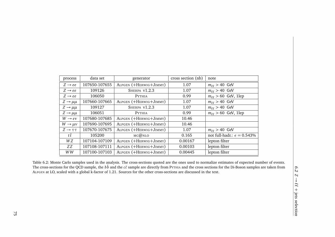
6.2Z→``+
jetsselection
process data set generator cross section (nb) note
Z → ee 107650-107655 ALPGEN (+HERWIG+JIMMY) 1.07 m`` > 40 GeVZ → ee 109126 SHERPA v1.2.3 1.07 m`` > 40 GeVZ → ee 106050 PYTHIA 0.99 m`` > 60 GeV, 1lepZ → µµ 107660-107665 ALPGEN (+HERWIG+JIMMY) 1.07 m`` > 40 GeVZ → µµ 109127 SHERPA v1.2.3 1.07 m`` > 40 GeVZ → µµ 106051 PYTHIA 0.99 m`` > 60 GeV, 1lepW → eν 107680-107685 ALPGEN (+HERWIG+JIMMY) 10.46W → µν 107690-107695 ALPGEN (+HERWIG+JIMMY) 10.46Z → ττ 107670-107675 ALPGEN (+HERWIG+JIMMY) 1.07 m`` > 40 GeV
t t 105200 MC@NLO 0.165 not full-hadr.: ε= 0.543%W Z 107104-107109 ALPGEN (+HERWIG+JIMMY) 0.00167 lepton filterZ Z 107108-107111 ALPGEN (+HERWIG+JIMMY) 0.00103 lepton filter
WW 107100-107103 ALPGEN (+HERWIG+JIMMY) 0.00445 lepton filter
Table 6.2: Monte Carlo samples used in the analysis. The cross-sections quoted are the ones used to normalize estimates of expected number of events.The cross-sections for the QCD sample, the bb and the cc sample are directly from PYTHIA and the cross sections for the Di-Boson samples are taken fromALPGEN at LO, scaled with a global k-factor of 1.21. Sources for the other cross-sections are discussed in the text.
75
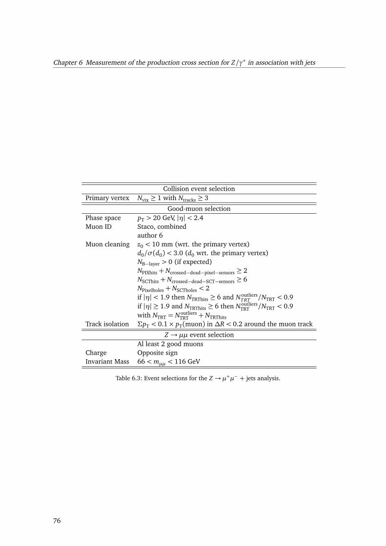
Chapter 6 Measurement of the production cross section for Z/γ∗ in association with jets
Collision event selectionPrimary vertex Nvtx ≥ 1 with Ntracks ≥ 3
Good-muon selectionPhase space pT > 20 GeV, |η|< 2.4Muon ID Staco, combined
author 6Muon cleaning z0 < 10 mm (wrt. the primary vertex)
d0/σ(d0)< 3.0 (d0 wrt. the primary vertex)NB−layer > 0 (if expected)NPIXhits+ Ncrossed−dead−pixel−sensors ≥ 2NSCThits+ Ncrossed−dead−SCT−sensors ≥ 6NPixelholes+ NSCTholes < 2if |η|< 1.9 then NTRThits ≥ 6 and Noutliers
TRT /NTRT < 0.9if |η| ≥ 1.9 and NTRThits ≥ 6 then Noutliers
TRT /NTRT < 0.9with NTRT = Noutliers
TRT + NTRThitsTrack isolation ΣpT < 0.1× pT(muon) in ∆R< 0.2 around the muon track
Z → µµ event selectionAl least 2 good muons
Charge Opposite signInvariant Mass 66< mµµ < 116 GeV
Table 6.3: Event selections for the Z → µ+µ− + jets analysis.
76
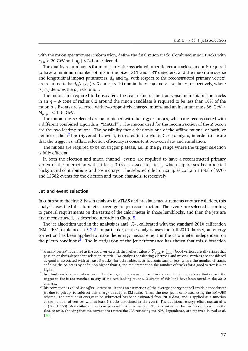
6.2 Z → `` + jets selection
with the muon spectrometer information, define the final muon track. Combined muon tracks withpTµ > 20 GeV and |ηµ|< 2.4 are selected.
The quality requirements for muons are: the associated inner detector track segment is requiredto have a minimum number of hits in the pixel, SCT and TRT detectors, and the muon transverseand longitudinal impact parameters, d0 and z0, with respect to the reconstructed primary vertex1
are required to be d0/σ(d0)< 3 and z0 < 10 mm in the r−φ and r− z planes, respectively, whereσ(d0) denotes the d0 resolution.
The muons are required to be isolated: the scalar sum of the transverse momenta of the tracksin an η−φ cone of radius 0.2 around the muon candidate is required to be less than 10% of themuon pT. Events are selected with two oppositely charged muons and an invariant mass 66 GeV<Mµ+µ− < 116 GeV.
The muon tracks selected are not matched with the trigger muons, which are reconstructed witha different combined algorithm (“MuGirl”). The muons used for the reconstruction of the Z bosonare the two leading muons. The possibility that either only one of the offline muons, or both, orneither of them2 has triggered the event, is treated in the Monte Carlo analysis, in order to ensurethat the trigger vs. offline selection efficiency is consistent between data and simulation.
The muons are required to be on trigger plateau, i.e. in the pT range where the trigger selectionis fully efficient.
In both the electron and muon channel, events are required to have a reconstructed primaryvertex of the interaction with at least 3 tracks associated to it, which suppresses beam-relatedbackground contributions and cosmic rays. The selected dilepton samples contain a total of 9705and 12582 events for the electron and muon channels, respectively.
Jet and event selection
In contrast to the first Z boson analyses in ATLAS and previous measurements at other colliders, thisanalysis uses the full calorimeter coverage for jet reconstruction. The events are selected accordingto general requirements on the status of the calorimeter in those lumiblocks, and then the jets arefirst reconstructed, as described already in Chap. 5.
The jet algorithm used in the analysis is anti−KT , calibrated with the standard 2010 calibration(EM+JES), explained in 5.2.2. In particular, as the analysis uses the full 2010 dataset, an energycorrection has been applied to make the energy measurement in the calorimeter independent onthe pileup conditions3. The investigation of the jet performance has shown that this subtraction
1“Primary vertex” is defined as the good vertex with the highest value of∑
tracks pT2,tracks. Good vertices are all vertices that
pass an analysis-dependent selection criteria. For analysis considering electrons and muons, vertices are consideredas good if associated with at least 3 tracks; for other objects, as hadronic taus or jets, where the number of tracksdefining the object is by definition higher than 3, the requirement on the number of tracks for a good vertex is 4 orhigher.
2This third case is a case where more than two good muons are present in the event: the muon track that caused thetrigger to fire is not matched to any of the two leading muons. 3 events of this kind have been found in the 2010analysis.
3This correction is called Jet Offset Correction. It uses an estimation of the average energy per cell inside a topoclusterjet due to pileup, to subtract this energy already at EM-scale. Then, the new jet is calibrated using the EM+JESscheme. The amount of energy to be subtracted has been estimated from 2010 data, and is applied as a functionof the number of vertices with at least 5 tracks associated in the event. The additional energy offset measured isof (500± 160) MeV within the jet cone per each extra interaction. The derivation of this correction, as well as theclosure tests, showing that the corrections restore the JES removing the NPV dependence, are reported in Aad et al.[10].
77
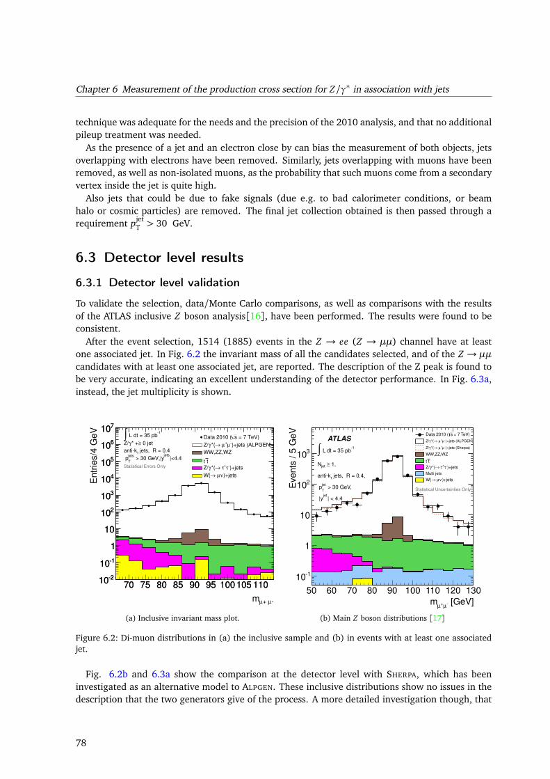
Chapter 6 Measurement of the production cross section for Z/γ∗ in association with jets
technique was adequate for the needs and the precision of the 2010 analysis, and that no additionalpileup treatment was needed.
As the presence of a jet and an electron close by can bias the measurement of both objects, jetsoverlapping with electrons have been removed. Similarly, jets overlapping with muons have beenremoved, as well as non-isolated muons, as the probability that such muons come from a secondaryvertex inside the jet is quite high.
Also jets that could be due to fake signals (due e.g. to bad calorimeter conditions, or beamhalo or cosmic particles) are removed. The final jet collection obtained is then passed through arequirement pjet
T > 30 GeV.
6.3 Detector level results
6.3.1 Detector level validation
To validate the selection, data/Monte Carlo comparisons, as well as comparisons with the resultsof the ATLAS inclusive Z boson analysis[16], have been performed. The results were found to beconsistent.
After the event selection, 1514 (1885) events in the Z → ee (Z → µµ) channel have at leastone associated jet. In Fig. 6.2 the invariant mass of all the candidates selected, and of the Z → µµcandidates with at least one associated jet, are reported. The description of the Z peak is found tobe very accurate, indicating an excellent understanding of the detector performance. In Fig. 6.3a,instead, the jet multiplicity is shown.
µ+ µm
70 75 80 85 90 95 100 105 110
Entr
ies/4
GeV
210
110
1
10
210
310
410
510
610
710
70 75 80 85 90 95 100 105 110210
110
1
10
210
310
410
510
610
710 = 7 TeV)sData 2010 (
)+jets (ALPGEN)µ+µ →*(γZ/
WW,ZZ,WZ
tt
)+jetsτ+τ →*(γZ/
)+jetsνµ →W(
1 L dt = 35 pb∫
0 jet≥* +γZ/
jets, R = 0.4tantik
|<4.4jets
> 30 GeV,|yjets
T p
Statistical Errors Only
(a) Inclusive invariant mass plot.
[GeV]µ+µm
50 60 70 80 90 100 110 120 130
Events
/ 5
GeV
110
1
10
210
310
ATLAS
1 L dt = 35 pb∫
1,≥ jetN
jets, R = 0.4,tantik
> 30 GeV,jet
T p
| < 4.4jet
|y
Statistical Uncertainties Only
= 7 TeV)sData 2010 (
)+jets (ALPGEN)µ+µ →*(γZ/
)+jets (Sherpa)µ+µ →*(γZ/
WW,ZZ,WZ
tt
)+jetsτ+τ →*(γZ/
Multi jets
)+jetsνµ →W(
(b) Main Z boson distributions [17]
Figure 6.2: Di-muon distributions in (a) the inclusive sample and (b) in events with at least one associatedjet.
Fig. 6.2b and 6.3a show the comparison at the detector level with SHERPA, which has beeninvestigated as an alternative model to ALPGEN. These inclusive distributions show no issues in thedescription that the two generators give of the process. A more detailed investigation though, that
78
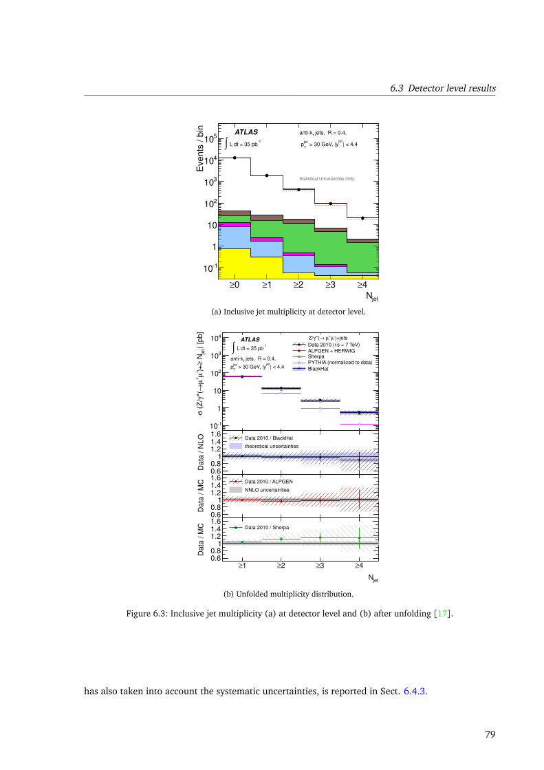
6.3 Detector level results
jetN
0≥ 1≥ 2≥ 3≥ 4≥
Events
/ b
in
110
1
10
210
310
410
510
ATLAS
1 L dt = 35 pb∫
jets, R = 0.4,tantik
| < 4.4jet
> 30 GeV, |yjet
T p
Statistical Uncertainties Only
(a) Inclusive jet multiplicity at detector level.
) [p
b]
jet
N≥)+
µ+
µ→
*(γ (
Z/
σ
110
1
10
210
310
410 = 7 TeV)sData 2010 (
ALPGEN + HERWIG Sherpa PYTHIA (normalized to data)
BlackHat
ATLAS )+jetsµ+µ →*(γZ/
1 L dt = 35 pb∫
jets, R = 0.4,tantik
| < 4.4jet
> 30 GeV, |yjet
Tp
Data
/ N
LO
0.60.8
11.21.41.6
Data 2010 / BlackHat
theoretical uncertainties
Data
/ M
C
0.60.8
11.21.41.6
Data 2010 / ALPGEN
NNLO uncertainties
jet N
1≥ 2≥ 3≥ 4≥
Data
/ M
C
0.60.8
11.21.41.6
Data 2010 / Sherpa
(b) Unfolded multiplicity distribution.
Figure 6.3: Inclusive jet multiplicity (a) at detector level and (b) after unfolding [17].
has also taken into account the systematic uncertainties, is reported in Sect. 6.4.3.
79
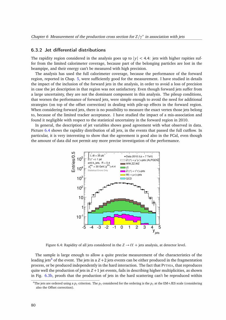
Chapter 6 Measurement of the production cross section for Z/γ∗ in association with jets
6.3.2 Jet differential distributions
The rapidity region considered in the analysis goes up to |y| < 4.4: jets with higher rapities suf-fer from the limited calorimeter coverage, because part of the belonging particles are lost in thebeampipe, and their energy can’t be measured with high precision.
The analysis has used the full calorimeter coverage, because the performance of the forwardregion, reported in Chap. 5, were sufficiently good for the measurement. I have studied in detailsthe impact of the inclusion of the forward jets in the analysis, in order to avoid a loss of precisionin case the jet description in that region was not satisfactory. Even though forward jets suffer froma large uncertainty, they are not the dominant component in this analysis. The pileup conditions,that worsen the performance of forward jets, were simple enough to avoid the need for additionalstrategies (on top of the offset correction) in dealing with pile-up effects in the forward region.When considering forward jets, there is no possibility to measure the exact vertex those jets belongto, because of the limited tracker acceptance. I have studied the impact of a mis-association andfound it negligible with respect to the statistical uncertainty in the forward region in 2010.
In general, the description of jet variables shows good agreement with what observed in data.Picture 6.4 shows the rapidity distribution of all jets, in the events that passed the full cutflow. Inparticular, it is very interesting to show that the agreement is good also in the FCal, even thoughthe amount of data did not permit any more precise investigation of the performance.
jetsy
5 4 3 2 1 0 1 2 3 4 5
En
trie
s/0
.5
110
1
10
210
310
410
510 = 7 TeV)sData 2010 (
)+jets (ALPGEN)µ+µ →*(γZ/
WW,ZZ,WZ
tt
)+jetsτ+τ →*(γZ/
)+jetsνµ →W(
QCD
1 L dt = 35 pb∫
1 jet≥* +γZ/
jets, R = 0.4tantik
|<4.4jets
> 30 GeV,|yjets
T p
Statistical Errors Only
Figure 6.4: Rapidity of all jets considered in the Z → `` + jets analysis, at detector level.
The sample is large enough to allow a quite precise measurement of the characteristics of theleading jets4 of the event. The jets in a Z+2 jets events can be either produced in the fragmentationprocess, or be produced independently in the hard interaction. The fact that PYTHIA, that reproducesquite well the production of jets in Z+1 jet events, fails in describing higher multiplicities, as shownin Fig. 6.3b, proofs that the production of jets in the hard scattering can’t be reproduced within
4The jets are ordered using a pT criterion. The pT considered for the ordering is the pT at the EM+JES scale (consideringalso the Offset correction).
80
6.4 Comparison with Monte Carlo LO and NLO pQCD predictions
a parton shower generator. The measurement of ∆y between the leading jets, a quantity highlysensitive to hadronization effects, shows that even those jets tend to be produced with a smallseparation in rapidity, as expected due to the color flow between the two partons in the productionprocess. In Fig. 6.5a the∆y is shown at detector level for a large range; Fig. 6.5b instead shows theresult at particle level, where the behavior of the jets produced only from a parton shower (PYTH-IA) shows clearly a not satisfying description of the data. The matrix element generators (ALPGEN
and SHERPA), instead, provide a more precise description of the jets in the event. The differencebetween SHERPA and the data at the core of the distribution provides also new inputs for the SHERPA
hadronization model, and is being studied by the authors. The difference at high rapidities willinstead be investigated further in future measurements.
In addition to those variables, the investigation of the rapidity gaps in Z → µ+µ− + jets eventshas considered also possible additional jets. Unfortunately, the statistics in 2010 was too low topermit a more sophisticated study. Fig. 6.6 shows one of these variables, Z∗(defined in Eq. 4.3),that puts in relation the rapidity of the leading jets with the rapidity of the third jet. Events with alow value of |Z∗| have additional jets in between the two leading jets of the event.
Consistent results have also been obtained in the electron channel. The two channels differmostly for the reconstruction and identification efficiencies, that explains the difference alreadymentioned in the number of Z → ee and Z → µµ events collected. Also the acceptance of the calo-rimeter and the muon spectrometer are different. For this reason, the analysis is kept separated intotwo channels at the particle level: because of the large difference in the efficiencies, the unfoldingcorrections for electrons are higher than those for muons. After unfolding, the two measurementshave been combined (after extrapolation to a common acceptance).
6.4 Comparison with Monte Carlo LO and NLO pQCDpredictions
Several uncertainties contribute to the measurement, dominated by the jet energy uncertainties.For the purpose of this thesis, they are also the most important and will be treated in more details.The details for the other uncertainties are in Aad et al. [17]; they consist of:
• leptons selection and reconstruction efficiencies: it includes uncertainties on the absoluteenergy scale and energy resolution, the uncertainty on the identification efficiency (only forelectrons), and the uncertainties on the reconstruction scale factors applied to the MC simu-lation. The trigger efficiency uncertainty has been found to be negligible;
• the QCD background uncertainty for Z → ee (for Z → µµ is found to be negligible).
6.4.1 Jet systematic uncertainties
Jet energy scale uncertainty
For the Z → `` + jets analysis the uncertainty in the central and forward region needs to be under-stood. This is provided by the jet in-situ analyses, as shown in Chap. 5. The results have shownthat the modelling, mostly for pT < 50 GeV, is suffering from large uncertainties, larger when thejet is reconstructed at high |η|.
The effect of a jet energy scale mismeasurement is visible in the number of jets counted in thedifferent jet bins. Given that the energy scale uncertainty for jets is moreover larger than the
81
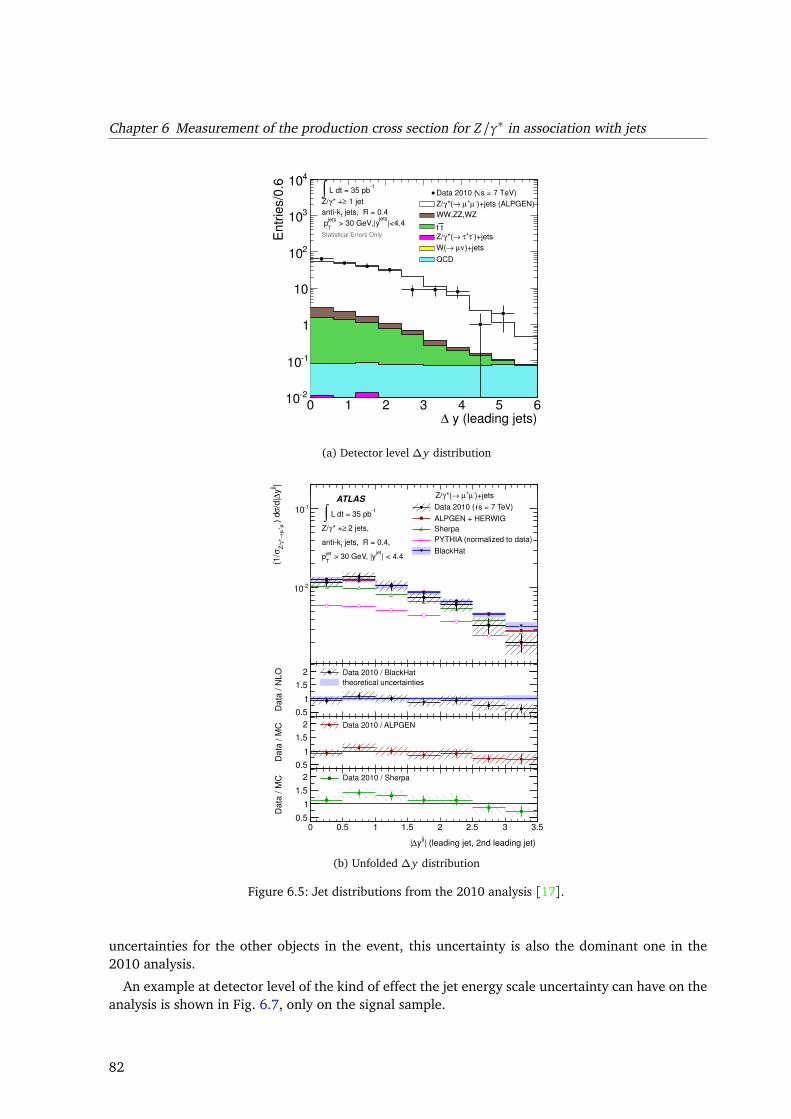
Chapter 6 Measurement of the production cross section for Z/γ∗ in association with jets
y (leading jets)∆0 1 2 3 4 5 6
Entr
ies/0
.6
210
110
1
10
210
310
410 = 7 TeV)sData 2010 (
)+jets (ALPGEN)µ+µ →*(γZ/
WW,ZZ,WZ
tt
)+jetsτ+τ →*(γZ/
)+jetsνµ →W(
QCD
1 L dt = 35 pb∫
1 jet≥* +γZ/
jets, R = 0.4tantik
|<4.4jets
> 30 GeV,|yjets
T p
Statistical Errors Only
(a) Detector level ∆y distribution
|jjy
∆/d
|σ
) d
µ
+µ
→*γZ
/σ
(1/
210
110 = 7 TeV)sData 2010 (
ALPGEN + HERWIG
Sherpa
PYTHIA (normalized to data)
BlackHat
ATLAS)+jetsµ+µ →*(γZ/
1 L dt = 35 pb∫
2 jets,≥* +γZ/
jets, R = 0.4,t
antik
| < 4.4jet
> 30 GeV, |yjet
Tp
Data
/ N
LO
0.5
1
1.5
2 Data 2010 / BlackHat
theoretical uncertainties
Data
/ M
C
0.5
1
1.5
2 Data 2010 / ALPGEN
| (leading jet, 2nd leading jet) jj
y∆|
0 0.5 1 1.5 2 2.5 3 3.5
Data
/ M
C
0.5
1
1.5
2 Data 2010 / Sherpa
(b) Unfolded ∆y distribution
Figure 6.5: Jet distributions from the 2010 analysis [17].
uncertainties for the other objects in the event, this uncertainty is also the dominant one in the2010 analysis.
An example at detector level of the kind of effect the jet energy scale uncertainty can have on theanalysis is shown in Fig. 6.7, only on the signal sample.
82
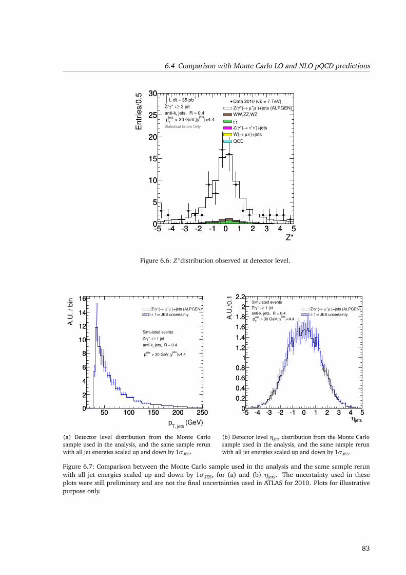
6.4 Comparison with Monte Carlo LO and NLO pQCD predictions
Z*5 4 3 2 1 0 1 2 3 4 5
En
trie
s/0
.5
0
5
10
15
20
25
30
5 4 3 2 1 0 1 2 3 4 50
5
10
15
20
25
30 = 7 TeV)sData 2010 (
)+jets (ALPGEN)µ+µ →*(γZ/
WW,ZZ,WZ
tt
)+jetsτ+τ →*(γZ/
)+jetsνµ →W(
QCD
1 L dt = 35 pb∫
3 jet≥* +γZ/
jets, R = 0.4tantik
|<4.4jets
> 30 GeV,|yjets
T p
Statistical Errors Only
Figure 6.6: Z∗distribution observed at detector level.
(GeV)T, jets
p
50 100 150 200 250
A.U
. / bin
0
2
4
6
8
10
12
14
16
50 100 150 200 2500
2
4
6
8
10
12
14
16
)+jets (ALPGEN)µ+µ →*(γZ/
JES uncertaintyσ 1 ±
Simulated events
1 jet≥* +γZ/
jets, R = 0.4tantik
|<4.4jets
> 30 GeV,|yjets
T p
(a) Detector level distribution from the Monte Carlosample used in the analysis, and the same sample rerunwith all jet energies scaled up and down by 1σJES.
jetsη5 4 3 2 1 0 1 2 3 4 5
A.U
./0.1
0
0.2
0.4
0.6
0.8
1
1.2
1.4
1.6
1.8
2
2.2
5 4 3 2 1 0 1 2 3 4 50
0.2
0.4
0.6
0.8
1
1.2
1.4
1.6
1.8
2
2.2
)+jets (ALPGEN)µ+µ →*(γZ/
JES uncertaintyσ 1 ±
Simulated events
1 jet≥* +γZ/
jets, R = 0.4tantik
|<4.4jets
> 30 GeV,|yjets
T p
(b) Detector level ηjets distribution from the Monte Carlosample used in the analysis, and the same sample rerunwith all jet energies scaled up and down by 1σJES.
Figure 6.7: Comparison between the Monte Carlo sample used in the analysis and the same sample rerunwith all jet energies scaled up and down by 1σJES, for (a) and (b) ηjets. The uncertainty used in theseplots were still preliminary and are not the final uncertainties used in ATLAS for 2010. Plots for illustrativepurpose only.
83
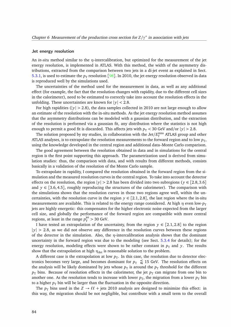
Chapter 6 Measurement of the production cross section for Z/γ∗ in association with jets
Jet energy resolution
An in-situ method similar to the η-intercalibration, but optimized for the measurement of the jetenergy resolution, is implemented in ATLAS. With this method, the width of the asymmetry dis-tributions, extracted from the comparison between two jets in a di-jet event as explained in Sect.5.3.1, is used to estimate the pT resolution [98]. In 2010, the jet energy resolution observed in datais reproduced well by the simulations used.
The uncertainties of the method used for the measurement in data, as well as any additionaleffect (for example, the fact that the resolution changes with rapidity, due to the different cell sizesin the calorimeter), need to be estimated to correctly take into account the resolution effects in theunfolding. These uncertainties are known for |y|< 2.8.
For high rapidities (|y| > 2.8), the data samples collected in 2010 are not large enough to allowan estimate of the resolution with the in-situ methods. As the jet energy resolution method assumesthat the asymmetry distributions can be modeled with a gaussian distribution, and the extractionof the resolution is performed via a gaussian fit, any distribution where the statistics is not highenough to permit a good fit is discarded. This affects jets with pT < 30 GeV and/or |y|> 2.8.
The solution proposed by my studies, in collaboration with the Jet/EmissT ATLAS group and other
ATLAS analyses, is to extrapolate the resolution measurements to the forward region and to low pT,using the knowledge developed in the central region and additional data–Monte Carlo comparison.
The good agreement between the resolution obtained in data and in simulations for the centralregion is the first point supporting this approach. The parametrization used is derived from simu-lation studies: thus, the comparison with data, and with results from different methods, consistsbasically in a validation of the resolution of the Monte Carlo sample.
To extrapolate in rapidity, I compared the resolution obtained in the forward region from the si-mulation and the measured resolution curves in the central region. To take into account the detectoreffects on the resolution, the region |y| > 2.8 has been divided into two subregions (y ∈ [2.8, 3.6]and y ∈ [3.6, 4.5], roughly reproducing the structures of the calorimeter). The comparison withthe simulations shows that the resolution curves in those two regions agree well, within the un-certainties, with the resolution curve in the region y ∈ [2.1, 2.8], the last region where the in-situmeasurements are available. This is related to the energy range considered. At high η even low-pTjets are highly energetic: this compensates for the higher electronic noise expected from the largercell size, and globally the performance of the forward region are compatible with more centralregions, at least in the range pjet
T > 30 GeV.I have tested an extrapolation of the uncertainty, from the region y ∈ [2.1,2.8] to the region
|y| > 2.8, as we did not observe any difference in the resolution curves between these regionsof the detector in the simulation. Also, the η-intercalibration analysis shows that the dominantuncertainty in the forward region was due to the modeling (see Sect. 5.3.4 for details); for theenergy resolution, modeling effects were shown to be rather constant in pT and y . The resultsshow that the extrapolation at high ηdet is reasonable solution to the problem.
A different case is the extrapolation at low pT. In this case, the resolution due to detector elec-tronics becomes very large, and becomes dominant for pT ¯ 15 GeV. The resolution effects onthe analysis will be likely dominated by jets whose pT is around the pT threshold for the differentpT bins. Because of resolution effects in the calorimeter, the jet pT can migrate from one bin toanother one. As the resolution tends to increase with lower pT, the migration from a lower pT binto a higher pT bin will be larger than the fluctuation in the opposite direction.
The pT bins used in the Z → `` + jets 2010 analysis are designed to minimize this effect: inthis way, the migration should be not negligible, but contribute with a small term to the overall
84
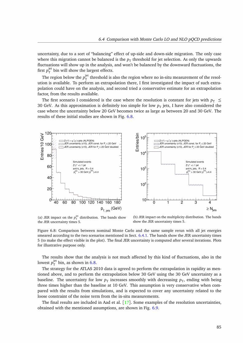
6.4 Comparison with Monte Carlo LO and NLO pQCD predictions
uncertainty, due to a sort of “balancing” effect of up-side and down-side migration. The only casewhere this migration cannot be balanced is the pT threshold for jet selection. As only the upwardsfluctuations will show up in the analysis, and won’t be balanced by the downward fluctuations, thefirst pjet
T bin will show the largest effects.
The region below the pjetT threshold is also the region where no in-situ measurement of the resol-
ution is available. To perform an extrapolation there, I first investigated the impact of such extra-polation could have on the analysis, and second tried a conservative estimate for an extrapolationfactor, from the results available.
The first scenario I considered is the case where the resolution is constant for jets with pT ≤30 GeV. As this approximation is definitely too simple for low pT jets, I have also considered thecase where the uncertainty below 20 GeV becomes twice as large as between 20 and 30 GeV. Theresults of these initial studies are shown in Fig. 6.8.
(GeV)T, jets
p
40 60 80 100 120 140 160 180
Entr
ies/1
0 G
eV
0
20
40
60
80
100
120
)+jets (ALPGEN)µ+µ →*(γZ/ 20 GeV≤
tJER uncertainty (x10), JER const. for P
20 GeV doubled≤ t
JER uncertainty (x10), JER for P
Simulated events
1 jet≥* +γZ/
jets, R = 0.4tantik
|<4.4jets
> 30 GeV,|yjets
T p
(a) JER impact on the pjetT distribution. The bands show
the JER uncertainty times 5.
jets N≥
0 1 2 3 4
Entr
ies/b
in
10
210
310
410
510
)+jets (ALPGEN)µ+µ →*(γZ/ 20 GeV≤
tJER uncertainty (x10), JER const. for P
20 GeV doubled≤ t
JER uncertainty (x10), JER for P
Simulated events
1 jet≥* +γZ/
jets, R = 0.4tantik
|<4.4jets
> 30 GeV,|yjets
T p
(b) JER impact on the multiplicity distribution. The bandsshow the JER uncertainty times 5.
Figure 6.8: Comparison between nominal Monte Carlo and the same sample rerun with all jet energiessmeared according to the two scenarios mentioned in Sect. 6.4.1. The bands show the JER uncertainty times5 (to make the effect visible in the plot). The final JER uncertainty is computed after several iterations. Plotsfor illustrative purpose only.
The results show that the analysis is not much affected by this kind of fluctuations, also in thelowest pjet
T bin, as shown in 6.8.The strategy for the ATLAS 2010 data is agreed to perform the extrapolation in rapidity as men-
tioned above, and to perform the extrapolation below 30 GeV using the 30 GeV uncertainty as abaseline. The uncertainty for low pT increases smoothly with decreasing pT, ending with beingthree times higher than the baseline at 10 GeV. This assumption is very conservative when com-pared with the results from simulations, and is expected to cover any uncertainty related to theloose constraint of the noise term from the in-situ measurements.
The final results are included in Aad et al. [17]. Some examples of the resolution uncertainties,obtained with the mentioned assumptions, are shown in Fig. 6.9.
85
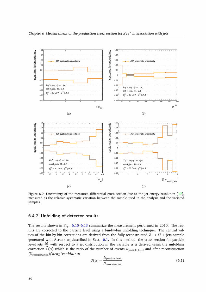
Chapter 6 Measurement of the production cross section for Z/γ∗ in association with jets
jet N≥
1 2 3 4
syste
matic u
ncert
ain
ty
0.95
0.96
0.97
0.98
0.99
1
1.01
1.02
1.03
1.04
1.05
JER systematic uncertainty
1 jet,≥) +µ µ →* ( γZ/
jets, R = 0.4t
antik
|<4.4jets
> 30 GeV, |yjets
Tp
(a)
jet
tp
40 60 80 100 120 140 160 180
syste
matic u
ncert
ain
ty
0.95
0.96
0.97
0.98
0.99
1
1.01
1.02
1.03
1.04
1.05
JER systematic uncertainty
1 jet,≥) +µ µ →* ( γZ/
jets, R = 0.4t
antik
|<4.4jets
> 30 GeV, |yjets
Tp
(b)
|jet
|y
0 0.5 1 1.5 2 2.5 3 3.5 4 4.5
syste
matic u
ncert
ain
ty
0.95
0.96
0.97
0.98
0.99
1
1.01
1.02
1.03
1.04
1.05
JER systematic uncertainty
1 jet,≥) +µ µ →* ( γZ/
jets, R = 0.4t
antik
|<4.4jets
> 30 GeV, |yjets
Tp
(c)
|leading jets
y∆|
0 1 2 3 4 5 6
syste
matic u
ncert
ain
ty
0.95
0.96
0.97
0.98
0.99
1
1.01
1.02
1.03
1.04
1.05
JER systematic uncertainty
2 jet,≥) +µ µ →* ( γZ/
jets, R = 0.4t
antik
|<4.4jets
> 30 GeV, |yjets
Tp
(d)
Figure 6.9: Uncertainty of the measured differential cross section due to the jet energy resolution [17],measured as the relative systematic variation between the sample used in the analysis and the variatedsamples.
6.4.2 Unfolding of detector results
The results shown in Fig. 6.10–6.13 summarize the measurement performed in 2010. The res-ults are corrected to the particle level using a bin-by-bin unfolding technique. The central val-ues of the bin-by-bin corrections are derived from the fully-reconstructed Z → `` + jets samplegenerated with ALPGEN as described in Sect. 6.1. In this method, the cross section for particlelevel jets dσ
dαwith respect to a jet distribution in the variable α is derived using the unfolding
correction U(α) which is the ratio of the number of events Nparticle level and after reconstruction(Nreconstructed) f oragivenbininα:
U(α) =Nparticle level
Nreconstructed(6.1)
86
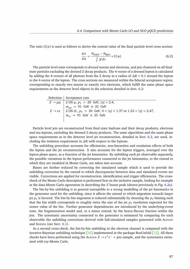
6.4 Comparison with Monte Carlo LO and NLO pQCD predictions
The ratio U(α) is used as follows to derive the central value of the final particle level cross section:
dσ
dα=
NDATA− NBKG∫
L d t∗ U(α) (6.2)
The particle level state corresponds to dressed muons and electrons, and jets clustered on all final-state particles excluding the dressed Z decay products. The 4-vector of a dressed lepton is calculatedby adding the 4-vectors of all photons from the Z decay in a radius of ∆R < 0.1 around the leptonto the 4-vector of the lepton. The cross sections are measured within the fiducial acceptance region,corresponding to exactly two muons or exactly two electrons, which fulfill the same phase spacerequirements as the detector level objects in the selection detailed in Sect. 6.2:
Selection Acceptance cutsZ → µµ 2 OS µ, pT > 20 GeV, |η|< 2.4,
mµµ = 91 GeV ± 25 GeVZ → ee 2 OS el., pT > 20 GeV, 0< |η|< 1.37 or 1.52< |η|< 2.47,
mee = 91 GeV ± 25 GeV
Particle level jets are reconstructed from final state hadrons and their decay products, electronsand tau-leptons, excluding the dressed Z-decay products. The same algorithms and the same phasespace requirements as in the detector level jet reconstruction, detailed in Sect. 6.2, are used, in-cluding the isolation requirement in ∆R with respect to the leptons.
The unfolding procedure accounts for efficiencies, non-linearities and resolution effects of boththe lepton and the jet reconstruction. It also accounts for the lepton triggers, averaged over thelepton phase space, as a function of the jet kinematics. By unfolding each jet observable separately,the possible variations in the lepton performance connected to the jet kinematics, to the extend towhich they are modeled in Monte Carlo, are taken into account.
Biases are further reduced by correcting the simulated sample which is used to provide theunfolding correction by the extend to which discrepancies between data and simulated events arevisible. Corrections are applied for reconstruction, identification and trigger efficiencies. The cross-check of the Monte Carlo description is performed first on the inclusive sample, looking for exampleat the data-Monte Carlo agreement in describing the Z boson peak (shown previously in Fig. 6.2a).
The bin-by-bin unfolding is in general susceptible to a wrong modelling of the jet kinematics inthe generator used for the unfolding, since it affects the extend to which migration towards largerjet pT is favored. The bin-by-bin migration is reduced substantially by choosing the pT binning suchthat the bin width corresponds to roughly twice the size of the jet pT resolution expected for thecenter value of the bin. Further generator dependencies are introduced by the underlying-eventtune, the fragmentation model and, to a minor extend, by the heavy-flavour fraction within thejets. The systematic uncertainty connected to the generator is estimated by comparing for eachobservable the unfolding corrections derived with full-simulated samples generated with ALPGEN
and SHERPA (see Sect. 6.1).As a second cross-check, the bin-by-bin unfolding in the electron channel is compared with the
iterative Bayesian unfolding technique [56] implemented in the package RooUnfold [33]. All thesechecks have been performed using the ALPGEN Z → e+e− + jets sample, and the systematics estim-ated with toy-Monte Carlo.
87
Chapter 6 Measurement of the production cross section for Z/γ∗ in association with jets
For each observable considered, cross sections are computed from the number NDATA of eventsselected in data according to the following prescription for the central value of a bin:
∆σ∆α=
NDATA− NBKG∫
L d t∗ U(α) ∗
1
∆α(6.3)
where U(α) is the bin-by-bin correction, which accounts for the unfolding from detector to particlelevel and NBKG is the predicted number of background events. The normalization to the bin-width∆α is also applied.
The correction factors vary between 1.3 and 1.6 in the electron channel, and between 1.1 and1.2 in the muon channel. The uncertainties range from 0.4 to 7%, increasing with higher jetmultiplicity, higher pjet
T or higher rapidity.The measured cross sections are compared at the particle level to predictions of the generators
ALPGEN and SHERPA, both normalized to the respective NNLO cross sections, and to predictions byPYTHIA Z → `` + jets, normalized to the average Z boson cross section in the electron and muonchannel observed in data. The data is also compared to perturbative QCD predictions at NLO byBLACKHAT (more details in Aad et al. [17]).
We observe an overall agreement of the ALPGEN and SHERPA predictions with the results observedin data. The pQCD predictions of BLACKHAT describe well the inclusive and differential cross sectionsmeasured in data.
6.4.3 Combination of electron and muon channel
The measured cross section distributions for the Z → ee+jets and Z → µµ+jets analyses are com-bined. The results present precise absolute jet cross section measurements.
The electron and muon measurements are performed in different fiducial regions for the rapidityof the leptons in the final state (see Table 6.4.2). In addition, the QED radiation effects are differentin both channels. For each measured distribution, bin-by-bin correction factors, as extracted fromALPGEN Z → ee+jets and Z → µµ+jets MC samples, are used to extrapolate the measurementsto the region pT > 20 GeV and |η| < 2.5 for the leptons, where the lepton kinematics are definedat the decay vertex of the Z boson. The increased acceptance in the lepton rapidities translatesinto about a 14% and a 5% increase of the measured cross sections in the electron and muonchannels, respectively. The correction for QED effects increases the cross sections by about 2%.The uncertainties on the acceptance corrections are at the per mille level, as determined by usingSHERPA instead of ALPGEN, and by considering different PDFs.
A χ2 test is performed for each observable to quantify the agreement between the electron andmuon results before they are combined, where the statistical and uncorrelated uncertainties aretaken into account. The statistical tests lead to probabilities larger than 60% for the electronand muon measurements to be compatible with each other, consistent with slightly conservativesystematic uncertainties. The electron and muon results are then combined using the BLUE (BestLinear Unbiased Estimate) [89] method, which considers the correlations between the systematicuncertainties in the two channels.
The measurements are well described by the BLACKHAT NLO pQCD predictions, and by the pre-dictions from ALPGEN and SHERPA. The corresponding χ2 tests relative to the different predictions,performed separately in each channel and for each observable, lead to χ2 per degree of freedomvalues in the range between 0.05 and 2.70. All correction factors and χ2 values are reported inAad et al. [17].
88
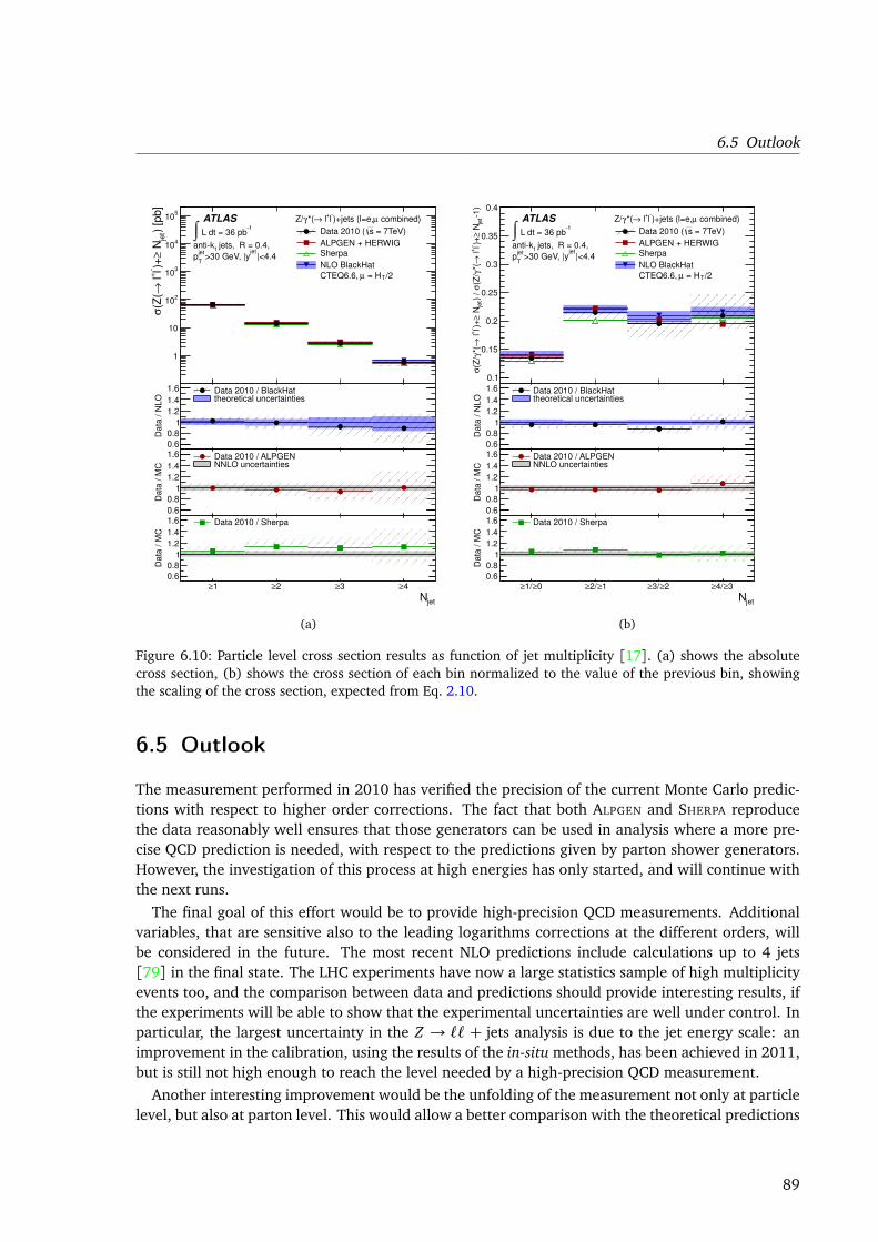
6.5 Outlook)
[pb]
jet
N≥
)+ l+ l
→(Z
(σ
1
10
210
310
410
510
1 L dt = 36 pb∫
jets, R = 0.4,tantik
|<4.4jet
>30 GeV, |yjet
Tp
combined)µ)+jets (l=e,l
+ l→*(γZ/ ATLAS
= 7TeV)sData 2010 (
ALPGEN + HERWIGSherpa
NLO BlackHat
= H /2 µCTEQ6.6, T
Data
/ N
LO
0.6
0.8
1
1.2
1.4
1.6 Data 2010 / BlackHattheoretical uncertainties
Data
/ M
C
0.6
0.8
1
1.2
1.4
1.6 Data 2010 / ALPGENNNLO uncertainties
jetN1≥ 2≥ 3≥ 4≥
Data
/ M
C
0.6
0.8
1
1.2
1.4
1.6 Data 2010 / Sherpa
(a)
1)
jet
N≥)+ l
+ l→
*(γ(Z
/σ
) /
jet
N≥)+ l
+ l→
*(γ(Z
/σ
0.1
0.15
0.2
0.25
0.3
0.35
0.4
1 L dt = 36 pb∫
jets, R = 0.4,tantik
|<4.4jet
>30 GeV, |yjet
Tp
combined)µ)+jets (l=e,l
+ l→*(γZ/ ATLAS
= 7TeV)sData 2010 (
ALPGEN + HERWIGSherpa
NLO BlackHat
= H /2 µCTEQ6.6, T
Data
/ N
LO
0.6
0.8
1
1.2
1.4
1.6 Data 2010 / BlackHattheoretical uncertainties
Data
/ M
C
0.6
0.8
1
1.2
1.4
1.6 Data 2010 / ALPGENNNLO uncertainties
jetN0≥1/≥ 1≥2/≥ 2≥3/≥ 3≥4/≥
Data
/ M
C
0.6
0.8
1
1.2
1.4
1.6 Data 2010 / Sherpa
(b)
Figure 6.10: Particle level cross section results as function of jet multiplicity [17]. (a) shows the absolutecross section, (b) shows the cross section of each bin normalized to the value of the previous bin, showingthe scaling of the cross section, expected from Eq. 2.10.
6.5 Outlook
The measurement performed in 2010 has verified the precision of the current Monte Carlo predic-tions with respect to higher order corrections. The fact that both ALPGEN and SHERPA reproducethe data reasonably well ensures that those generators can be used in analysis where a more pre-cise QCD prediction is needed, with respect to the predictions given by parton shower generators.However, the investigation of this process at high energies has only started, and will continue withthe next runs.
The final goal of this effort would be to provide high-precision QCD measurements. Additionalvariables, that are sensitive also to the leading logarithms corrections at the different orders, willbe considered in the future. The most recent NLO predictions include calculations up to 4 jets[79] in the final state. The LHC experiments have now a large statistics sample of high multiplicityevents too, and the comparison between data and predictions should provide interesting results, ifthe experiments will be able to show that the experimental uncertainties are well under control. Inparticular, the largest uncertainty in the Z → `` + jets analysis is due to the jet energy scale: animprovement in the calibration, using the results of the in-situ methods, has been achieved in 2011,but is still not high enough to reach the level needed by a high-precision QCD measurement.
Another interesting improvement would be the unfolding of the measurement not only at particlelevel, but also at parton level. This would allow a better comparison with the theoretical predictions
89
Chapter 6 Measurement of the production cross section for Z/γ∗ in association with jets
and with the measurement performed at other experiments.A comparison between the two general-purpose experiments at the LHC, ATLAS and CMS, would
be very useful also for Monte Carlo tuning. At the moment, the measurements at the two ex-periments are only performed within the acceptance region, and use different generators for thedata-Monte Carlo comparison. The first could be overcome by an extrapolation, and the latter,in principle, could be an advantage, since a combination or a comparison between the two experi-ments could shed light on the behaviour of different parton shower and underlying event generatorsin a similar environment. The comparison between the two experiments is however not straight-forward. The physics objects are defined differently, as expected from two different detectors. Insome cases (e.g. the leptons), the difference could be absorbed into the acceptance corrections. Incontrast, the choice of a different size of the jet algorithm (anti−KT with parameter 0.4 for ATLAS,0.5 for CMS [111]) can’t be easily re-absorbed and makes the comparison harder. It is clear that allthe quantities measured have a dependence on the algorithm definition, while in the pQCD regime,that is the final goal of a precision Z → `` + jets measurement, any such dependence should notbe visible. Even defining a “pure” pQCD regime will be challenging: the analysis should be able todemonstrate that it is not sensitive to fragmentation, underlying event, and other effects that occurat lower energy scales. Reaching such a precision will not be matter of integrated luminosity, but itwill need a joint effort of both the experimental and the theory community working on QCD studiesat LHC.
90
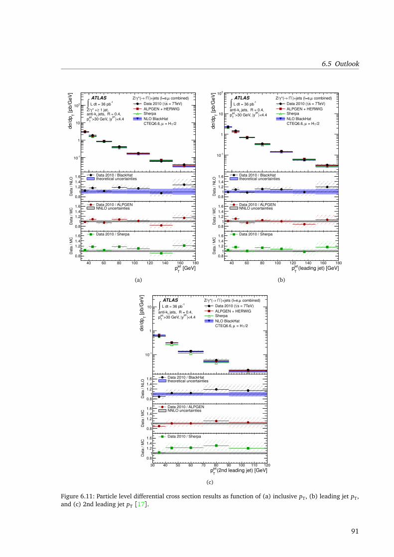
6.5 Outlook [pb/G
eV
]T
/dp
σd
110
1
10
210
1 L dt = 36 pb∫
1 jet,≥* +γZ/ jets, R = 0.4,tantik
|<4.4jet
>30 GeV, |yjet
Tp
combined)µ)+jets (l=e,l
+ l→*(γZ/ ATLAS
= 7TeV)sData 2010 (
ALPGEN + HERWIGSherpa
NLO BlackHat
= H /2 µCTEQ6.6, T
Data
/ N
LO
0.8
1
1.2
1.4
1.6 Data 2010 / BlackHattheoretical uncertainties
Data
/ M
C
0.8
1
1.2
1.4
1.6 Data 2010 / ALPGENNNLO uncertainties
[GeV]jet
Tp
40 60 80 100 120 140 160 180
Data
/ M
C
0.8
1
1.2
1.4
1.6 Data 2010 / Sherpa
(a)
[pb/G
eV
]T
/dp
σd
110
1
10
210
1 L dt = 36 pb∫
jets, R = 0.4,tantik
|<4.4jet
>30 GeV, |yjet
Tp
combined)µ)+jets (l=e,l
+ l→*(γZ/ ATLAS
= 7TeV)sData 2010 (
ALPGEN + HERWIGSherpa
NLO BlackHat
= H /2 µCTEQ6.6, T
Data
/ N
LO
0.8
1
1.2
1.4
1.6 Data 2010 / BlackHattheoretical uncertainties
Data
/ M
C
0.8
1
1.2
1.4
1.6 Data 2010 / ALPGENNNLO uncertainties
(leading jet) [GeV]jet
Tp
40 60 80 100 120 140 160 180
Data
/ M
C
0.8
1
1.2
1.4
1.6 Data 2010 / Sherpa
(b)
[pb/G
eV
]T
/dp
σd
110
1
101
L dt = 36 pb∫ jets, R = 0.4,tantik
|<4.4jet
>30 GeV, |yjet
Tp
combined)µ)+jets (l=e,l
+ l→*(γZ/ ATLAS
= 7TeV)sData 2010 (
ALPGEN + HERWIGSherpa
NLO BlackHat
= H /2 µCTEQ6.6, T
Data
/ N
LO
0.8
1
1.2
1.4
1.6 Data 2010 / BlackHattheoretical uncertainties
Data
/ M
C
0.8
1
1.2
1.4
1.6 Data 2010 / ALPGENNNLO uncertainties
(2nd leading jet) [GeV]jet
Tp
30 40 50 60 70 80 90 100 110 120
Data
/ M
C
0.8
1
1.2
1.4
1.6 Data 2010 / Sherpa
(c)
Figure 6.11: Particle level differential cross section results as function of (a) inclusive pT, (b) leading jet pT,and (c) 2nd leading jet pT [17].
91
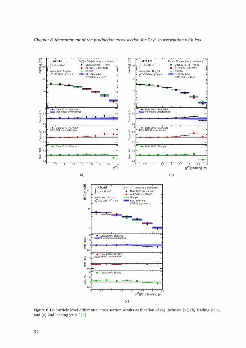
Chapter 6 Measurement of the production cross section for Z/γ∗ in association with jets/d
|y| [p
b]
σd
1
10
210
310
1 L dt = 36 pb∫
jets, R = 0.4,tantik
|<4.4jet
>30 GeV, |yjet
Tp
combined)µ)+jets (l=e,l
+ l→*(γZ/ ATLAS
= 7TeV)sData 2010 (
ALPGEN + HERWIGSherpa
NLO BlackHat
= H /2 µCTEQ6.6, T
Data
/ N
LO
0.5
1
1.5
2 Data 2010 / BlackHattheoretical uncertainties
Data
/ M
C
0.5
1
1.5
2 Data 2010 / ALPGENNNLO uncertainties
|jet
|y
0 0.5 1 1.5 2 2.5 3 3.5 4
Data
/ M
C
0.5
1
1.5
2 Data 2010 / Sherpa
(a)
/d|y
| [p
b]
σd
1
10
210
310
1 L dt = 36 pb∫
jets, R = 0.4,tantik
|<4.4jet
>30 GeV, |yjet
Tp
combined)µ)+jets (l=e,l
+ l→*(γZ/ ATLAS
= 7TeV)sData 2010 (
ALPGEN + HERWIGSherpa
NLO BlackHat
= H /2 µCTEQ6.6, T
Data
/ N
LO
0.5
1
1.5
2 Data 2010 / BlackHattheoretical uncertainties
Data
/ M
C
0.5
1
1.5
2 Data 2010 / ALPGENNNLO uncertainties
|(leading jet)jet
|y
0 0.5 1 1.5 2 2.5 3 3.5 4
Data
/ M
C
0.5
1
1.5
2 Data 2010 / Sherpa
(b)
/d|y
| [p
b]
σd
1
10
210 1
L dt = 36 pb∫ jets, R = 0.4,tantik
|<4.4jet
>30 GeV, |yjet
Tp
combined)µ)+jets (l=e,l
+ l→*(γZ/ ATLAS
= 7TeV)sData 2010 (
ALPGEN + HERWIGSherpa
NLO BlackHat
= H /2 µCTEQ6.6, T
Data
/ N
LO
0.5
1
1.5
2 Data 2010 / BlackHattheoretical uncertainties
Data
/ M
C
0.5
1
1.5
2 Data 2010 / ALPGENNNLO uncertainties
|(2nd leading jet)jet
|y
0 0.5 1 1.5 2 2.5 3 3.5
Data
/ M
C
0.5
1
1.5
2 Data 2010 / Sherpa
(c)
Figure 6.12: Particle level differential cross section results as function of (a) inclusive |y|, (b) leading jet y ,and (c) 2nd leading jet y [17].
92
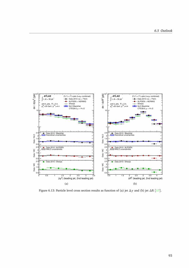
6.5 Outlook| [p
b]
jjy
∆ / d
|σ
d
1
10
210
1 L dt = 36 pb∫
jets, R = 0.4,tantik
|<4.4jet
>30 GeV, |yjet
Tp
combined)µ)+jets (l=e,l
+ l→*(γZ/ ATLAS
= 7TeV)sData 2010 (
ALPGEN + HERWIGSherpa
NLO BlackHat
= H /2 µCTEQ6.6, T
Data
/ N
LO
0.5
1
1.5
2
2.5 Data 2010 / BlackHattheoretical uncertainties
Data
/ M
C
0.5
1
1.5
2
2.5 Data 2010 / ALPGENNNLO uncertainties
| (leading jet, 2nd leading jet) jj
y∆|0 0.5 1 1.5 2 2.5 3 3.5
Data
/ M
C
0.5
1
1.5
2
2.5 Data 2010 / Sherpa
(a)
[pb]
jjR
∆ / d
σd
1
10
210
1 L dt = 36 pb∫
jets, R = 0.4,tantik
|<4.4jet
>30 GeV, |yjet
Tp
combined)µ)+jets (l=e,l
+ l→*(γZ/ ATLAS
= 7TeV)sData 2010 (
ALPGEN + HERWIGSherpa
NLO BlackHat
= H /2 µCTEQ6.6, T
Data
/ N
LO
0.5
1
1.5
2
2.5 Data 2010 / BlackHattheoretical uncertainties
Data
/ M
C
0.5
1
1.5
2
2.5 Data 2010 / ALPGENNNLO uncertainties
(leading jet, 2nd leading jet)jj
R∆0.5 1 1.5 2 2.5 3 3.5 4
Data
/ M
C
0.5
1
1.5
2
2.5 Data 2010 / Sherpa
(b)
Figure 6.13: Particle level cross section results as function of (a) jet ∆y and (b) jet ∆R [17].
93

Chapter 7
Search for the Standard Model Higgsboson in the τ+τ− channel
7.1 Strategy
In this chapter, the results of the searches for the Higgs boson performed in 2011 with the ATLASdetector in the H → ττ channel, on a sample corresponding to an integrated luminosity of 4.7 fb−1,are reported. I have contributed to the search in the final state with electrons and muons, theH → ττ→ ``+ 4ν process.
The importance of this channel in the SM Higgs searches has already been highlighted in Sect.2.4. τ leptons have a large branching fraction both in leptons and in hadrons, thus the possibilityto detect this channel with good efficiency are high. The final state into electrons and muonsis in particular very clean, and can benefit from the good ATLAS reconstruction performance forthese physics objects. But, as mentioned in Sect. 2.4.2, several other effects play a role in theexperimental search, and can make the extraction of the signal harder.
The dominant backgrounds for the H → ττ→ ``+ 4ν analysis are:
• Z → ττ: this is the dominant irreducible background to the H → ττ signal. The final statecharacteristics are the same, and the main visible difference between the two events will bedepending on the characteristics of the production channels, different for Z → ττ and H →ττ, and on the Higgs mass. Exploiting the first information requires knowing how the partonlevel final state can propagate to the detector level according to the production mechanismand additional effects, as hadronization (see Sect. 7.2). The detection of the Higgs mass peakon the Z → ττ peak tail relies on the mass reconstruction and resolution. Techniques thatallow a good mass reconstruction using the Emiss
T information are used: in particular, we haveused the collinear approximation (see Sect. 7.5). For this reason, in Z → ττ the modelling ofthe Emiss
T description is of fundamental importance.
• Z → `` (e,µ): the difference between this background and the H → ττ signal is related to theEmiss
T , because true EmissT is present only in H → ττ events and not in Z → `` events. For this
reason, any experimental effect on the EmissT description will be crucial in the discrimination
between this background and the signal. Concerning the description of the Z → `` kinemat-ics, the modelling given by Monte Carlo is in agreement with the measurements shown inChap. 6, and no issues are expected in this case.
• W → `ν + jets: this background is important because it has a large cross section and itsprobability to pass the selection depends on the mis-identification rate. In these events onelepton comes from the leptonic decay of the W boson, while the other one comes from a jetidentified as a lepton, or from leptons produced in hadronic cascades (as caused by heavy
95
Chapter 7 Search for the Standard Model Higgs boson in the τ+τ− channel
flavour production) but mis-identified as isolated leptons because of a bad reconstruction ofthe cascade. The mis-identification rate is difficult both to measure with high precision andto reproduce with Monte Carlo.
• top quark production: these events can provide a quite large source of background, becausethey can include both real jets and real leptons coming from the W boson decay. The possib-ility to reject this background, however, are quite high because of the good performance ofthe b-taggers used in ATLAS.
Considering these large backgrounds, it is of fundamental importance to develop a strategy thatallows a successful rejection of the background while keeping a high signal efficiency. The strategyused in the ATLAS analysis is based on two different goals, highlighted in the following.
Higher discrimination between signal and background in events with jets: the H → ττfinal state is characterised by a back-to-back configuration of the two τ leptons in the Higgs bosonrest frame. The leptons originating in the leptonic decay are boosted in the direction of the decayingτ and have small opening angles with respect to such direction. If the Higgs boson is producedin absence of additional particles with high transverse momentum, the event is characterised bya small Emiss
T in the laboratory rest frame. In this case, the signal to background ratio will betoo small for a successful search, because of the large Z → `` background and the difficulties indistinguishing between the two topologies.
If in the event extra jets with high transverse momentum are produced, the Higgs boson acquiresa boost in the transverse plane. This enhances the transverse momenta of the Higgs decay productsand, as a consequence, the Emiss
T of the event. This topology can be better distinguished frombackground processes, as shown by Mellado, Quayle and Wu [93]. However, previous analyses inATLAS [29], simply requiring the presence of an additional jet in the event, did not show a verylarge improvement of the significance; a more careful investigation of the jet topology was neededto achieve the goal. This is the main aim of the investigation performed on 2011 data.
The presence of additional radiation, and its characteristics, depend on the production processof the Higgs boson, as shown in Sect. 7.2. Using the information on both the production and decayof the Higgs, we can optimize the selection and enhance the sensitivity of the analysis. The 2011ATLAS analysis has decided to consider all production processes of the Higgs relevant for the lowmass region and to combine the results in the limit, instead of focussing on a single productionchannel (as was done in preliminary studies, e.g. on simulations [9], and in Chap. 4). Exploitingthe jet multiplicity, it is possible to divide the analysis in different jet bins, and to optimize theselection in each bin according to the dominant signal and background processes.
Using my previous experience with the Z → `` + jets analysis, I have investigated the descriptionof several jet variables important for the Higgs analysis. Z → `` + jets events provide a goodcontrol sample, as the signal contamination is expected to be negligible. At the same time, I havealso studied how to make the jet selection robust with respect to experimental effects, such as pile-up, that are difficult to reproduce in Monte Carlo and are highly affecting the 2011 run, as shownin Fig. 3.3. The results are reported in Sect. 7.4.1, and provide an important input to the definitionof the event selection cuts used in this analysis, summarized in Sect. 7.4.
EmissT modelling in the background: as stated already, the background description needs to be
cross-checked in data. The most careful checks concern the EmissT description, as the estimate of the
invariant di-τ mass depends on its performance. A summary of the methods used for Z → ``, t t,
96
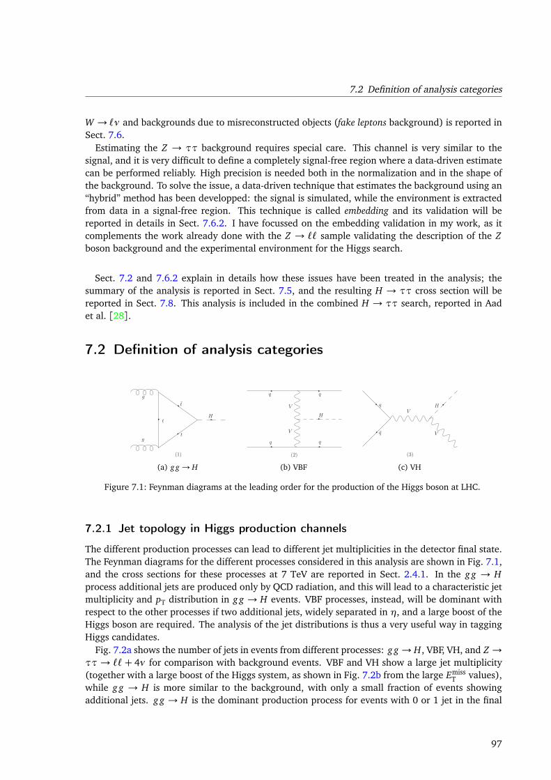
7.2 Definition of analysis categories
W → `ν and backgrounds due to misreconstructed objects (fake leptons background) is reported inSect. 7.6.
Estimating the Z → ττ background requires special care. This channel is very similar to thesignal, and it is very difficult to define a completely signal-free region where a data-driven estimatecan be performed reliably. High precision is needed both in the normalization and in the shape ofthe background. To solve the issue, a data-driven technique that estimates the background using an“hybrid” method has been developped: the signal is simulated, while the environment is extractedfrom data in a signal-free region. This technique is called embedding and its validation will bereported in details in Sect. 7.6.2. I have focussed on the embedding validation in my work, as itcomplements the work already done with the Z → `` sample validating the description of the Zboson background and the experimental environment for the Higgs search.
Sect. 7.2 and 7.6.2 explain in details how these issues have been treated in the analysis; thesummary of the analysis is reported in Sect. 7.5, and the resulting H → ττ cross section will bereported in Sect. 7.8. This analysis is included in the combined H → ττ search, reported in Aadet al. [28].
7.2 Definition of analysis categories
gt
g
H
t
(1)
t
(a) g g → H
q
H
q
q
(2)
q
V
V
(b) VBF
V
q
H
V
q
(3)
(c) VH
Figure 7.1: Feynman diagrams at the leading order for the production of the Higgs boson at LHC.
7.2.1 Jet topology in Higgs production channels
The different production processes can lead to different jet multiplicities in the detector final state.The Feynman diagrams for the different processes considered in this analysis are shown in Fig. 7.1,and the cross sections for these processes at 7 TeV are reported in Sect. 2.4.1. In the g g → Hprocess additional jets are produced only by QCD radiation, and this will lead to a characteristic jetmultiplicity and pT distribution in g g → H events. VBF processes, instead, will be dominant withrespect to the other processes if two additional jets, widely separated in η, and a large boost of theHiggs boson are required. The analysis of the jet distributions is thus a very useful way in taggingHiggs candidates.
Fig. 7.2a shows the number of jets in events from different processes: g g → H, VBF, VH, and Z →ττ→ ``+ 4ν for comparison with background events. VBF and VH show a large jet multiplicity(together with a large boost of the Higgs system, as shown in Fig. 7.2b from the large Emiss
T values),while g g → H is more similar to the background, with only a small fraction of events showingadditional jets. g g → H is the dominant production process for events with 0 or 1 jet in the final
97
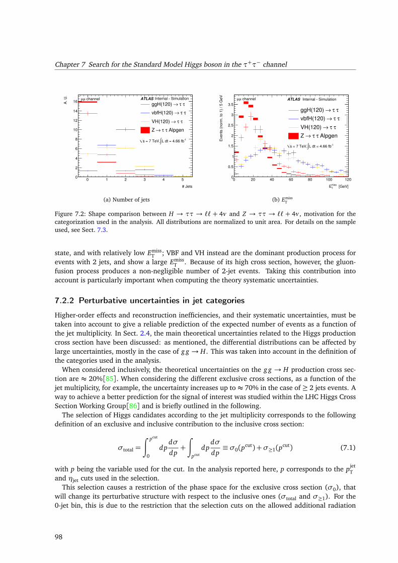
Chapter 7 Search for the Standard Model Higgs boson in the τ+τ− channel
# Jets
0 1 2 3 4 5
A.
U.
0
2
4
6
8
10
12
14
16τ τ →ggH(120)
τ τ →vbfH(120)
τ τ →VH(120)
Alpgenτ τ →Z
channelµµ
1L dt = 4.66 fb∫ = 7 TeV, s
ATLAS Internal Simulation
(a) Number of jets
[GeV]T
missE
0 20 40 60 80 100 120
Eve
nts
(n
orm
. to
1)
/ 5
Ge
V
0
0.5
1
1.5
2
2.5
3
3.5
τ τ →ggH(120)
τ τ →vbfH(120)
τ τ →VH(120)
Alpgenτ τ →Z
channelµµ
1L dt = 4.66 fb∫ = 7 TeV, s
ATLAS Internal Simulation
(b) EmissT
Figure 7.2: Shape comparison between H → ττ → `` + 4ν and Z → ττ → `` + 4ν , motivation for thecategorization used in the analysis. All distributions are normalized to unit area. For details on the sampleused, see Sect. 7.3.
state, and with relatively low EmissT ; VBF and VH instead are the dominant production process for
events with 2 jets, and show a large EmissT . Because of its high cross section, however, the gluon-
fusion process produces a non-negligible number of 2-jet events. Taking this contribution intoaccount is particularly important when computing the theory systematic uncertainties.
7.2.2 Perturbative uncertainties in jet categories
Higher-order effects and reconstruction inefficiencies, and their systematic uncertainties, must betaken into account to give a reliable prediction of the expected number of events as a function ofthe jet multiplicity. In Sect. 2.4, the main theoretical uncertainties related to the Higgs productioncross section have been discussed: as mentioned, the differential distributions can be affected bylarge uncertainties, mostly in the case of g g → H. This was taken into account in the definition ofthe categories used in the analysis.
When considered inclusively, the theoretical uncertainties on the g g → H production cross sec-tion are ≈ 20%[85]. When considering the different exclusive cross sections, as a function of thejet multiplicity, for example, the uncertainty increases up to ≈ 70% in the case of ≥ 2 jets events. Away to achieve a better prediction for the signal of interest was studied within the LHC Higgs CrossSection Working Group[86] and is briefly outlined in the following.
The selection of Higgs candidates according to the jet multiplicity corresponds to the followingdefinition of an exclusive and inclusive contribution to the inclusive cross section:
σtotal =
∫ pcut
0
dpdσ
dp+
∫
pcut
dpdσ
dp≡ σ0(p
cut) +σ≥1(pcut) (7.1)
with p being the variable used for the cut. In the analysis reported here, p corresponds to the pjetT
and ηjet cuts used in the selection.This selection causes a restriction of the phase space for the exclusive cross section (σ0), that
will change its perturbative structure with respect to the inclusive ones (σtotal and σ≥1). For the0-jet bin, this is due to the restriction that the selection cuts on the allowed additional radiation
98
7.2 Definition of analysis categories
applies to the collinear initial-state radiation as well as the overall soft radiation in the event. Thisrestriction causes large Sudakov-logarithms to appear: the cancellation that occurs in the inclusivecross sections, which ensures the convergence of the series (as for example in the case treated inSect. 2.3), does not happen any longer. Similar effects play a role in any definition of an exclusivejet cross section, independently from the number of jets considered.
If we try then to estimate the uncertainty on the cross section due to the missing higher orderdiagrams via scale variations (varying the renormalization and factorization scale in the fixed orderprediction, as it is commonly done for QCD processes), we might not get meaningful results dueto the influence of these logarithms on the calculations. This issue affects strongly the g g → Hproduction channel, while, for example, has a negligible effect on the Z → `` + jets process.
Because quantities are well defined in an inclusive cross section, the solution of the problemlies in the possibility of using the uncertainties on σtotal and σ≥1 (that can be estimated by scalevariations) to extract the uncertainty onσ0. It can be shown that, in the simple example mentioned,the uncertainty on σ0 can be estimated by error propagation from the uncertainty on the twoinclusive cross sections.
This simple example can easily be extended to additional jet-bins and cuts, provided that:
1. the inclusive cross sections are known up to the order needed to the calculation and are alltreated consistently;
2. the cuts used divide the phase space in mutually exclusive regions.
While the second item is easily satisfied in the analysis, the first one is challenging. In fact, for ag g → H analysis:
• σtotal is known at NNLO;
• σ≥N is known at N2−N LO;
• because NNLO corrections are large, there will be a non-negligible ambiguity in the definitionof the exclusive cross section rates: predictions show large differences depending if they aredefined from σ≥N or σ≥N−1.
From these considerations, it is clear where the large increase in the uncertainty of the g g → Hcross section comes from: if σ0,σ1,σ≥2 are the different jet categories, the uncertainty on σ≥2,available only at LO, will largely affect the result, as well as introducing a dangerous source ofambiguity in the definition. All these effects are related to the poor convergence of the perturbativeseries. To avoid those large uncertainties and improve the discrimination of the signal, additionalselection cuts as rapidity gaps and invariant mass cuts have been used to enhance the contributionof VBF and VH production processes.
Exploiting VBF and VH topologies, which are predicted with a better precision in those jet bins,increases the sensitivity to the signal. The uncertainties available for the H+2 jets cross section areavailable at NLO (see Sect. 7.3). g g → H events will still be present in those jet bins, but theywill not dominate the signal distribution. The gluon fusion uncertainty will be used in treatingthe correlation with the other exclusive bins, as the definition of the 1-jet bin and of the 2-jetbins are anti-correlated. But if 2-jet bins are well defined in the phase space via additional cuts,and all events that don’t pass those cuts are recovered in the 1-jet bin, no ambiguity is left in thedefinition of the cross sections, and the uncertainty can be treated consistently using the g g → Huncertainties at NLO.
99
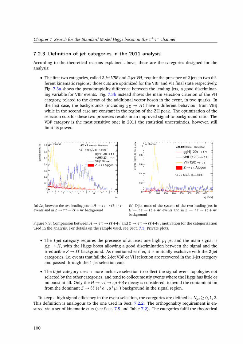
Chapter 7 Search for the Standard Model Higgs boson in the τ+τ− channel
7.2.3 Definition of jet categories in the 2011 analysis
According to the theoretical reasons explained above, these are the categories designed for theanalysis:
• The first two categories, called 2-jet VBF and 2-jet VH, require the presence of 2 jets in two dif-ferent kinematic regions: those cuts are optimized for the VBF and VH final state respectively.Fig. 7.3a shows the pseudorapidity difference between the leading jets, a good discriminat-ing variable for VBF events. Fig. 7.3b instead shows the main selection criterion of the VHcategory, related to the decay of the additional vector boson in the event, in two quarks. Inthe first case, the backgrounds (including g g → H) have a different behaviour from VBF,while in the second case are constant in the region of the ZH peak. The optimization of theselection cuts for these two processes results in an improved signal-to-background ratio. TheVBF category is the most sensitive one; in 2011 the statistical uncertainties, however, stilllimit its power.
η∆
0 1 2 3 4 5 6 7 8 9
Eve
nts
(n
orm
. to
1)
0
0.1
0.2
0.3
0.4
0.5
0.6
0.7
τ τ →ggH(120)
τ τ →vbfH(120)
τ τ →VH(120)
Alpgenτ τ →Z
channelµµ
1L dt = 4.66 fb∫ = 7 TeV, s
ATLAS Internal Simulation
(a)∆η between the two leading jets in H → ττ→ ``+4νevents and in Z → ττ→ ``+ 4ν background
[GeV]jjM
50 100 150 200 250 300 350 400
Eve
nts
(n
orm
. to
1)
/ 5
Ge
V
0
0.2
0.4
0.6
0.8
1
τ τ →ggH(120)
τ τ →vbfH(120)
τ τ →VH(120)
Alpgenτ τ →Z
channelµµ
1L dt = 4.66 fb∫ = 7 TeV, s
ATLAS Internal Simulation
(b) Dijet mass of the system of the two leading jets inH → ττ → `` + 4ν events and in Z → ττ → `` + 4νbackground
Figure 7.3: Comparison between H → ττ→ ``+4ν and Z → ττ→ ``+4ν , motivation for the categorizationused in the analysis. For details on the sample used, see Sect. 7.3. Private plots.
• The 1-jet category requires the presence of at least one high pT jet and the main signal isg g → H, with the Higgs boost allowing a good discrimination between the signal and theirreducible Z → `` background. As mentioned earlier, it is mutually exclusive with the 2-jetcategories, i.e. events that fail the 2-jet VBF or VH selection are recovered in the 1-jet categoryand passed through the 1-jet selection cuts.
• The 0-jet category uses a more inclusive selection to collect the signal event topologies notselected by the other categories, and tend to collect mostly events where the Higgs has little orno boost at all. Only the H → ττ→ eµ+ 4ν decay is considered, to avoid the contaminationfrom the dominant Z → `` (e+e−,µ+µ−) background in the signal region.
To keep a high signal efficiency in the event selection, the categories are defined as Njet ≥ 0,1, 2.This definition is analogous to the one used in Sect. 7.2.2. The orthogonality requirement is en-sured via a set of kinematic cuts (see Sect. 7.5 and Table 7.2). The categories fulfil the theoretical
100
7.3 Data and simulated samples
requirement highlighted earlier, thus ensure a better control of the prediction, and provide a bettersensitivity with respect to an inclusive analysis.
7.3 Data and simulated samples
Data The results are based on proton-proton collision data collected with ATLAS in 2011, at acentre-of-mass energy of
ps = 7 TeV. Only data taken with all sub-systems relevant to this analysis
operational are used. This results in an integrated luminosity of 4.7 fb−1 for the full 2011 datasample.
Higgs boson production: The cross-sections for Higgs boson production are calculated follow-ing the prescriptions of the LHC Higgs cross-section working group [86]. For the gluon fusionprocess, it has been calculated using HIGLU [107] and ggh@nnlo [72] at next-to-next to leadingorder (NNLO). For the vector boson fusion, the NLO calculation was performed with VBF@NLO [44,86]. For the associated production with vector bosons, the cross-section calculation is performed atNNLO QCD + NLO electro-weak (EW) scale [48, 53].
The SM Higgs boson production via gluon fusion is simulated with POWHEG [97] and the g g → Hevents were re-weighted as a function of the Higgs transverse momentum as prescribed by the LHCHiggs cross-section working group [86]. The VBF production of the Higgs boson was also simulatedwith POWHEG, while the associated production with vector boson was simulated with PYTHIA [105].
Z → `` + jets and Z → ττ → `` + 4ν production: The cross-section for Z → `` + jets iscalculated in NNLO QCD using the FEWZ code [64]. The Z → `` background is is simulated withthe ALPGEN [90] generator, using the same settings used in Chap. 6. This background is alsochecked on data, in particular for checking the normalization and the modelling of Emiss
T along thetails.
A data-driven approach is instead used to determine the Z → ττ → `` + 4ν contribution, asexplained in Sect. 7.6.2. The validation is performed against the relevant ALPGEN sample.
W → `ν + jets production: The cross-section is calculated in NNLO QCD using the FEWZ code.However, because this background is dominated by mis-identification effects, known with littleaccuracy, a data-driven approach is used to determine the contribution of this background. It isincluded in the so-called Fake leptons background.
Di-boson production: The electroweak production of pairs of vector bosons (WW , W Z , Z Z)can lead to final states with two or more charged leptons from the leptonic decays of the W and Zbosons. The cross-section is calculated at NLO with MC@NLO[63]. The di-boson (WW , W Z , Z Z)production processes are generated with HERWIG [54].
t t production: The cross-section is calculated in NLO+Next-to-Next-to-Leading Logarithmic(NNLL) QCD. The t t process is generated with MC@NLO, and a cross-check of the normalization isdone on data, looking at a t t enriched control region.
101
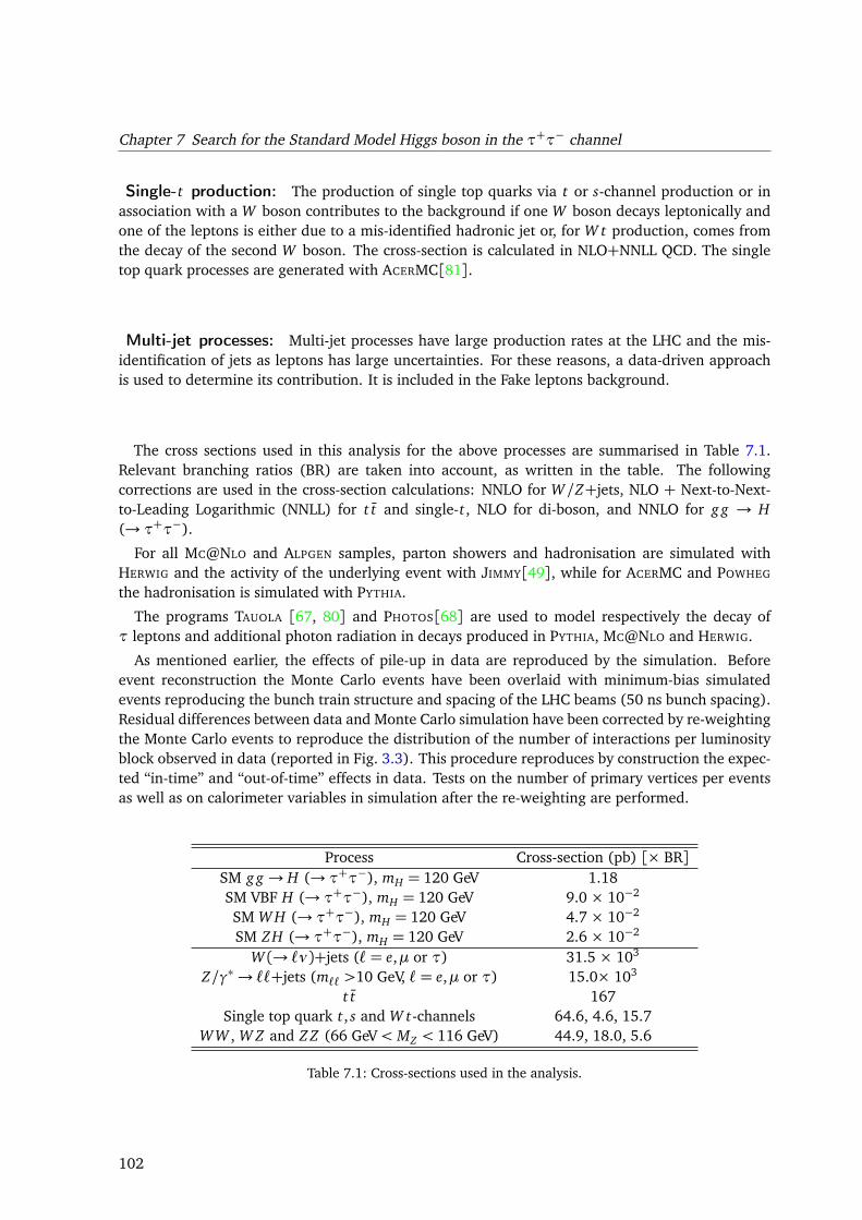
Chapter 7 Search for the Standard Model Higgs boson in the τ+τ− channel
Single-t production: The production of single top quarks via t or s-channel production or inassociation with a W boson contributes to the background if one W boson decays leptonically andone of the leptons is either due to a mis-identified hadronic jet or, for W t production, comes fromthe decay of the second W boson. The cross-section is calculated in NLO+NNLL QCD. The singletop quark processes are generated with ACERMC[81].
Multi-jet processes: Multi-jet processes have large production rates at the LHC and the mis-identification of jets as leptons has large uncertainties. For these reasons, a data-driven approachis used to determine its contribution. It is included in the Fake leptons background.
The cross sections used in this analysis for the above processes are summarised in Table 7.1.Relevant branching ratios (BR) are taken into account, as written in the table. The followingcorrections are used in the cross-section calculations: NNLO for W/Z+jets, NLO + Next-to-Next-to-Leading Logarithmic (NNLL) for t t and single-t, NLO for di-boson, and NNLO for g g → H(→ τ+τ−).
For all MC@NLO and ALPGEN samples, parton showers and hadronisation are simulated withHERWIG and the activity of the underlying event with JIMMY[49], while for ACERMC and POWHEG
the hadronisation is simulated with PYTHIA.
The programs TAUOLA [67, 80] and PHOTOS[68] are used to model respectively the decay ofτ leptons and additional photon radiation in decays produced in PYTHIA, MC@NLO and HERWIG.
As mentioned earlier, the effects of pile-up in data are reproduced by the simulation. Beforeevent reconstruction the Monte Carlo events have been overlaid with minimum-bias simulatedevents reproducing the bunch train structure and spacing of the LHC beams (50 ns bunch spacing).Residual differences between data and Monte Carlo simulation have been corrected by re-weightingthe Monte Carlo events to reproduce the distribution of the number of interactions per luminosityblock observed in data (reported in Fig. 3.3). This procedure reproduces by construction the expec-ted “in-time” and “out-of-time” effects in data. Tests on the number of primary vertices per eventsas well as on calorimeter variables in simulation after the re-weighting are performed.
Process Cross-section (pb) [× BR]SM g g → H (→ τ+τ−), mH = 120 GeV 1.18SM VBF H (→ τ+τ−), mH = 120 GeV 9.0 × 10⁻²
SM W H (→ τ+τ−), mH = 120 GeV 4.7 × 10⁻²
SM ZH (→ τ+τ−), mH = 120 GeV 2.6 × 10⁻²
W (→ `ν)+jets (`= e,µ or τ) 31.5 × 10³
Z/γ∗→ ``+jets (m`` >10 GeV, `= e,µ or τ) 15.0× 10³
t t 167Single top quark t, s and W t-channels 64.6, 4.6, 15.7
WW , W Z and Z Z (66 GeV< MZ < 116 GeV) 44.9, 18.0, 5.6
Table 7.1: Cross-sections used in the analysis.
102
7.4 Selection and reconstruction of physics objects
7.4 Selection and reconstruction of physics objects
Electrons: Electron candidates are formed from an energy deposit in the electromagnetic calo-rimeter and associated to a track measured in the inner detector. They are selected if they have atransverse energy ET > 15 GeV, lie within |η| < 2.47 but outside the transition region between thebarrel and end-cap calorimeters (1.37 < |η| < 1.52), and meet quality requirements based on theexpected shower shape [8].
Muons: Muon candidates are formed from a track measured in the inner detector and linkedto a track in the muon spectrometer [14]. They are required to have a transverse momentumpT > 10 GeV and to lie within |η| < 2.5. Additionally, the difference between the z-position of thepoint of closest approach of the muon inner detector track to the beam-line and the z-coordinateof the primary vertex is required to be less than 1 cm. This requirement reduces the contaminationdue to cosmic ray muons and beam-induced backgrounds. Muon quality criteria based on, e.g.,inner detector hit requirements are applied in order to achieve a precise measurement of the muonmomentum and reduce the misidentification rate. The preselection requirements are very similarto those used in the Z → `` + jets analysis; only some cuts have been relaxed to improve theefficiency of the preselection.
Isolation: Identified electrons and muons are required to be isolated: the additional transverseenergy in the electromagnetic and hadronic calorimeters must be less than 8% (4%) of the electrontransverse energy (muon transverse momentum) in a cone of radius ∆R=
p
(∆η)2+ (∆φ)2 = 0.2around the electron (muon) direction. The sum of the transverse momenta of all tracks with pTabove 1 GeV located within a cone of radius ∆R = 0.4 around the electron (muon) direction andoriginating from the same primary vertex must be less than 6% of the electron transverse energy(muon transverse momentum).
Jets: Jets are reconstructed using the anti−KT algorithm with a distance parameter value ofR= 0.4, taking topoclusters as input. Reconstructed jets with pT > 20 GeV and within |η|< 4.5 areselected. Events are discarded if a jet is associated with out-of-time activity or calorimeter noise.The jets are calibrated using calibration constants derived from the combination of the data/MonteCarlo comparison of the in-situ calibrations.
Jet vertex fraction: After having associated tracks to jets by requiring ∆R< 0.4 between tracksand the jet direction, a jet-vertex fraction (JVF) is computed for each jet as the scalar pT sum of allassociated tracks from the primary vertex divided by the scalar pT sum of all tracks associated withthe jet. Conventionally, JVF = −1 is assigned to jets with no associated tracks. Jets with
η
< 2.4are required to have |JVF| > 0.75 in order to suppress pileup contributions. The reasons behindthis selection criterion are reported in Sect. 7.4.1.
B-Jets rejection: In the pseudorapidity range
η
< 2.5, b-jets are identified using a tagging al-gorithm based on the discrimination power of the impact parameter information and of the recon-struction of the displaced vertices of the hadron decays inside the jets [7]. The b-tagging algorithmhas an average efficiency of 58% for b-jets in t t events [15]. The corresponding light-quark jetmisidentification probability is 0.1–0.5%, depending on the jet pT and η [13].
103
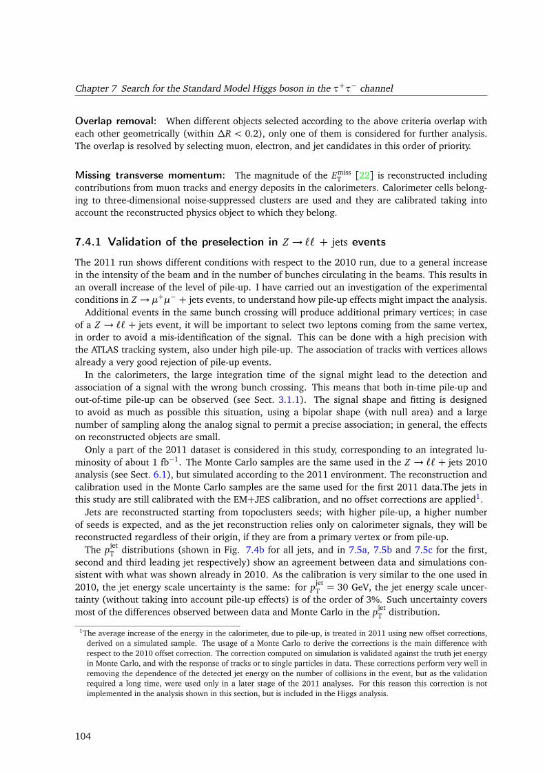
Chapter 7 Search for the Standard Model Higgs boson in the τ+τ− channel
Overlap removal: When different objects selected according to the above criteria overlap witheach other geometrically (within ∆R < 0.2), only one of them is considered for further analysis.The overlap is resolved by selecting muon, electron, and jet candidates in this order of priority.
Missing transverse momentum: The magnitude of the EmissT [22] is reconstructed including
contributions from muon tracks and energy deposits in the calorimeters. Calorimeter cells belong-ing to three-dimensional noise-suppressed clusters are used and they are calibrated taking intoaccount the reconstructed physics object to which they belong.
7.4.1 Validation of the preselection in Z → `` + jets events
The 2011 run shows different conditions with respect to the 2010 run, due to a general increasein the intensity of the beam and in the number of bunches circulating in the beams. This results inan overall increase of the level of pile-up. I have carried out an investigation of the experimentalconditions in Z → µ+µ− + jets events, to understand how pile-up effects might impact the analysis.
Additional events in the same bunch crossing will produce additional primary vertices; in caseof a Z → `` + jets event, it will be important to select two leptons coming from the same vertex,in order to avoid a mis-identification of the signal. This can be done with a high precision withthe ATLAS tracking system, also under high pile-up. The association of tracks with vertices allowsalready a very good rejection of pile-up events.
In the calorimeters, the large integration time of the signal might lead to the detection andassociation of a signal with the wrong bunch crossing. This means that both in-time pile-up andout-of-time pile-up can be observed (see Sect. 3.1.1). The signal shape and fitting is designedto avoid as much as possible this situation, using a bipolar shape (with null area) and a largenumber of sampling along the analog signal to permit a precise association; in general, the effectson reconstructed objects are small.
Only a part of the 2011 dataset is considered in this study, corresponding to an integrated lu-minosity of about 1 fb−1. The Monte Carlo samples are the same used in the Z → `` + jets 2010analysis (see Sect. 6.1), but simulated according to the 2011 environment. The reconstruction andcalibration used in the Monte Carlo samples are the same used for the first 2011 data.The jets inthis study are still calibrated with the EM+JES calibration, and no offset corrections are applied1.
Jets are reconstructed starting from topoclusters seeds; with higher pile-up, a higher numberof seeds is expected, and as the jet reconstruction relies only on calorimeter signals, they will bereconstructed regardless of their origin, if they are from a primary vertex or from pile-up.
The pjetT distributions (shown in Fig. 7.4b for all jets, and in 7.5a, 7.5b and 7.5c for the first,
second and third leading jet respectively) show an agreement between data and simulations con-sistent with what was shown already in 2010. As the calibration is very similar to the one used in2010, the jet energy scale uncertainty is the same: for pjet
T = 30 GeV, the jet energy scale uncer-tainty (without taking into account pile-up effects) is of the order of 3%. Such uncertainty coversmost of the differences observed between data and Monte Carlo in the pjet
T distribution.
1The average increase of the energy in the calorimeter, due to pile-up, is treated in 2011 using new offset corrections,derived on a simulated sample. The usage of a Monte Carlo to derive the corrections is the main difference withrespect to the 2010 offset correction. The correction computed on simulation is validated against the truth jet energyin Monte Carlo, and with the response of tracks or to single particles in data. These corrections perform very well inremoving the dependence of the detected jet energy on the number of collisions in the event, but as the validationrequired a long time, were used only in a later stage of the 2011 analyses. For this reason this correction is notimplemented in the analysis shown in this section, but is included in the Higgs analysis.
104
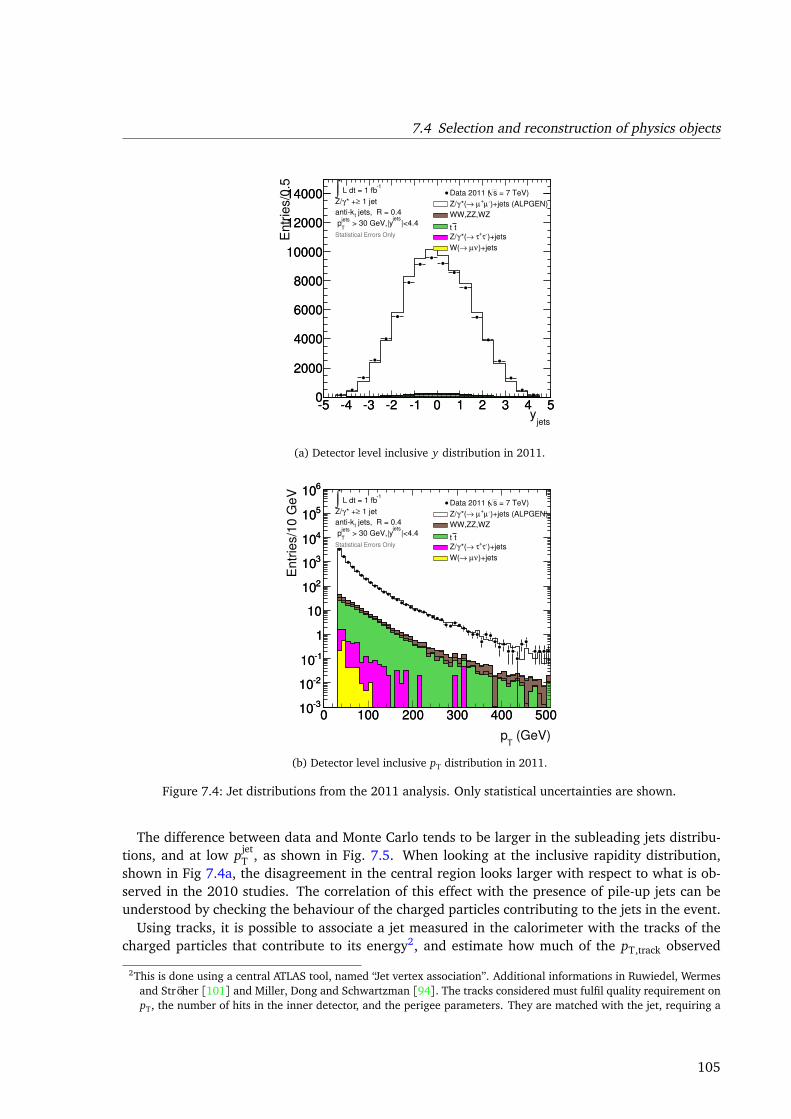
7.4 Selection and reconstruction of physics objects
jetsy
5 4 3 2 1 0 1 2 3 4 5
Entr
ies/0
.5
0
2000
4000
6000
8000
10000
12000
14000
5 4 3 2 1 0 1 2 3 4 50
2000
4000
6000
8000
10000
12000
14000 = 7 TeV)sData 2011 (
)+jets (ALPGEN)µ+µ →*(γZ/
WW,ZZ,WZ
tt
)+jetsτ+τ →*(γZ/
)+jetsνµ →W(
1 L dt = 1 fb∫
1 jet≥* +γZ/
jets, R = 0.4tantik
|<4.4jets
> 30 GeV,|yjets
T p
Statistical Errors Only
(a) Detector level inclusive y distribution in 2011.
(GeV)T
p
0 100 200 300 400 500
Entr
ies/1
0 G
eV
310
210
110
1
10
210
310
410
510
610
0 100 200 300 400 500310
210
110
1
10
210
310
410
510
610
= 7 TeV)sData 2011 (
)+jets (ALPGEN)µ+µ →*(γZ/
WW,ZZ,WZ
tt
)+jetsτ+τ →*(γZ/
)+jetsνµ →W(
1 L dt = 1 fb∫
1 jet≥* +γZ/
jets, R = 0.4tantik
|<4.4jets
> 30 GeV,|yjets
T p
Statistical Errors Only
(b) Detector level inclusive pT distribution in 2011.
Figure 7.4: Jet distributions from the 2011 analysis. Only statistical uncertainties are shown.
The difference between data and Monte Carlo tends to be larger in the subleading jets distribu-tions, and at low pjet
T , as shown in Fig. 7.5. When looking at the inclusive rapidity distribution,shown in Fig 7.4a, the disagreement in the central region looks larger with respect to what is ob-served in the 2010 studies. The correlation of this effect with the presence of pile-up jets can beunderstood by checking the behaviour of the charged particles contributing to the jets in the event.
Using tracks, it is possible to associate a jet measured in the calorimeter with the tracks of thecharged particles that contribute to its energy2, and estimate how much of the pT,track observed
2This is done using a central ATLAS tool, named “Jet vertex association”. Additional informations in Ruwiedel, Wermesand Ströher [101] and Miller, Dong and Schwartzman [94]. The tracks considered must fulfil quality requirement onpT, the number of hits in the inner detector, and the perigee parameters. They are matched with the jet, requiring a
105
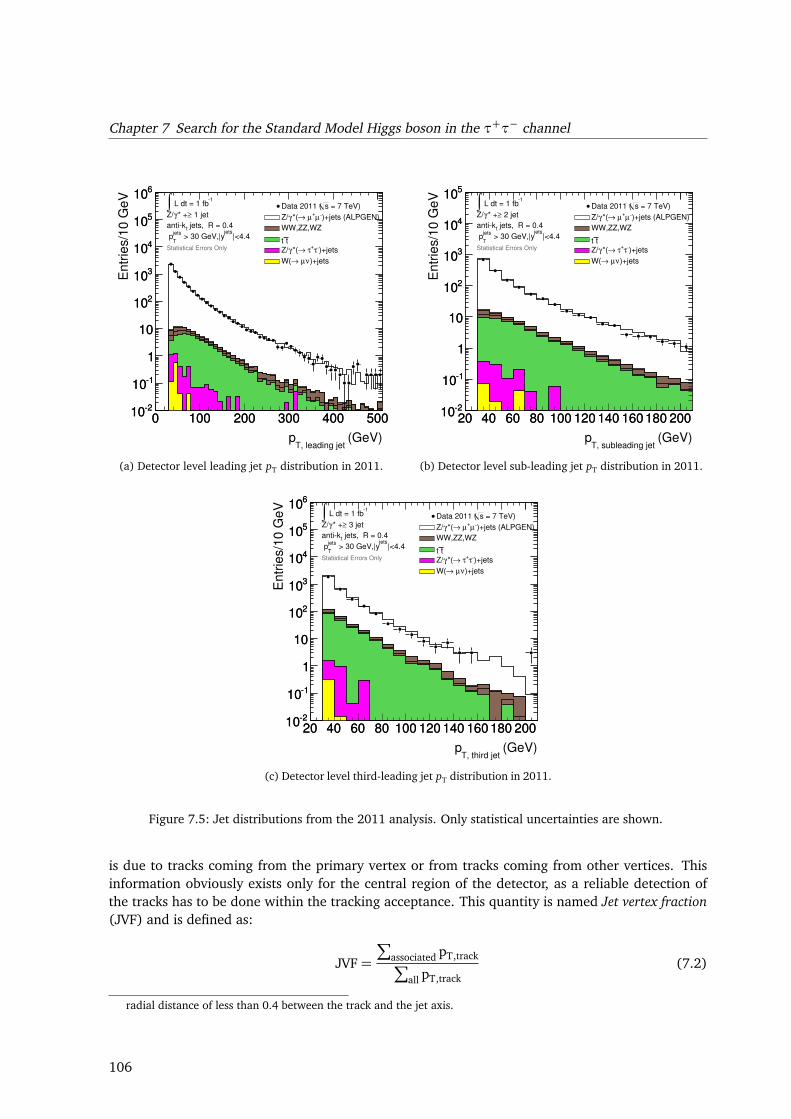
Chapter 7 Search for the Standard Model Higgs boson in the τ+τ− channel
(GeV)T, leading jet
p
0 100 200 300 400 500
Entr
ies/1
0 G
eV
210
110
1
10
210
310
410
510
610
0 100 200 300 400 500210
110
1
10
210
310
410
510
610
= 7 TeV)sData 2011 (
)+jets (ALPGEN)µ+µ →*(γZ/
WW,ZZ,WZ
tt
)+jetsτ+τ →*(γZ/
)+jetsνµ →W(
1 L dt = 1 fb∫
1 jet≥* +γZ/
jets, R = 0.4tantik
|<4.4jets
> 30 GeV,|yjets
T p
Statistical Errors Only
(a) Detector level leading jet pT distribution in 2011.
(GeV)T, subleading jet
p
20 40 60 80 100 120 140 160 180 200E
ntr
ies/1
0 G
eV
210
110
1
10
210
310
410
510
20 40 60 80 100 120 140 160 180 200210
110
1
10
210
310
410
510
= 7 TeV)sData 2011 (
)+jets (ALPGEN)µ+µ →*(γZ/
WW,ZZ,WZ
tt
)+jetsτ+τ →*(γZ/
)+jetsνµ →W(
1 L dt = 1 fb∫
2 jet≥* +γZ/
jets, R = 0.4tantik
|<4.4jets
> 30 GeV,|yjets
T p
Statistical Errors Only
(b) Detector level sub-leading jet pT distribution in 2011.
(GeV)T, third jet
p
20 40 60 80 100 120 140 160 180 200
Entr
ies/1
0 G
eV
210
110
1
10
210
310
410
510
610
20 40 60 80 100 120 140 160 180 200210
110
1
10
210
310
410
510
610
= 7 TeV)sData 2011 (
)+jets (ALPGEN)µ+µ →*(γZ/
WW,ZZ,WZ
tt
)+jetsτ+τ →*(γZ/
)+jetsνµ →W(
1 L dt = 1 fb∫
3 jet≥* +γZ/
jets, R = 0.4tantik
|<4.4jets
> 30 GeV,|yjets
T p
Statistical Errors Only
(c) Detector level third-leading jet pT distribution in 2011.
Figure 7.5: Jet distributions from the 2011 analysis. Only statistical uncertainties are shown.
is due to tracks coming from the primary vertex or from tracks coming from other vertices. Thisinformation obviously exists only for the central region of the detector, as a reliable detection ofthe tracks has to be done within the tracking acceptance. This quantity is named Jet vertex fraction(JVF) and is defined as:
JVF=
∑
associated pT,track∑
all pT,track(7.2)
radial distance of less than 0.4 between the track and the jet axis.
106
7.4 Selection and reconstruction of physics objects
0 0.2 0.4 0.6 0.8 1
Entr
ies/0
.031
210
110
1
10
210
310
410
510
610
710
810
0 0.2 0.4 0.6 0.8 1210
110
1
10
210
310
410
510
610
710
810
Jet Vertex Fraction0 0.2 0.4 0.6 0.8 1
σ
/
∆
10505
0 0.2 0.4 0.6 0.8 110505
= 7 TeV)sData 2011 (
)+jets (ALPGEN)µ+µ →*(γZ/
WW,ZZ,WZ
tt
)+jetsτ+τ →*(γZ/
)+jetsνµ →W(
1 L dt = 1 fb∫
1 jet≥* +γZ/
jets, R = 0.4tantik
|<4.4jets
> 30 GeV,|yjets
T p
Statistical Errors Only
Figure 7.6: Detector level Jet-Vertex-Fraction (JVF) distribution in 2011. Only statistical uncertainties areshown.
The distribution in 2011 data of the JVF is shown in Fig. 7.6.The JVF is usually computed with respect to the primary vertex of the event. From Eq. 7.2, it is
clear that jets made of particles coming from the primary vertex will tend to have a JVF close toone, while lower JVF values mean that the number of tracks contributing to the jet from the othervertices is very high, and their contribution to the total pT is higher than the one of the particlescoming from the primary vertex. As the method relies on tracking, two things must be taken intoaccount:
• the neutral particle contribution is not considered
• the JVF is limited to the tracking acceptance, |η|< 2.5
• jets with ηjet > 2.5 and jets within the tracking acceptance but that could not be associatedto any good quality track automatically get JVF=−1 (not shown in Fig. 7.6).
Even considering these limitations, the JVF is a useful quantity to understand the effects of pile-up in the central region of the detector. Fig. 7.4a shows a disagreement between data and theMonte Carlo predictions that is not fully consistent with the one in the pT distributions showed inFig. 7.5a, 7.5b and 7.5c. Looking at the JVF distribution in Fig. 7.6, the difference seems to bedominating in the low JVF distribution, where pile-up effects play a very large role. This meansthat the description of pile-up in 2011 is not completely reproducing the data; but, as those effectsseems to not to show up much in the pT distribution of the leading jets of the event, this means thatthe badly modeled population is mostly composed of low-pT jets.
I checked this hypothesis in data and developed a strategy for improving the selection using theJVF variable. A cut of |JVF| > 0.75 was added to the selection cuts, chosen in a region wherethe JVF is well described and the difference between data and Monte Carlo is roughly flat, such
107
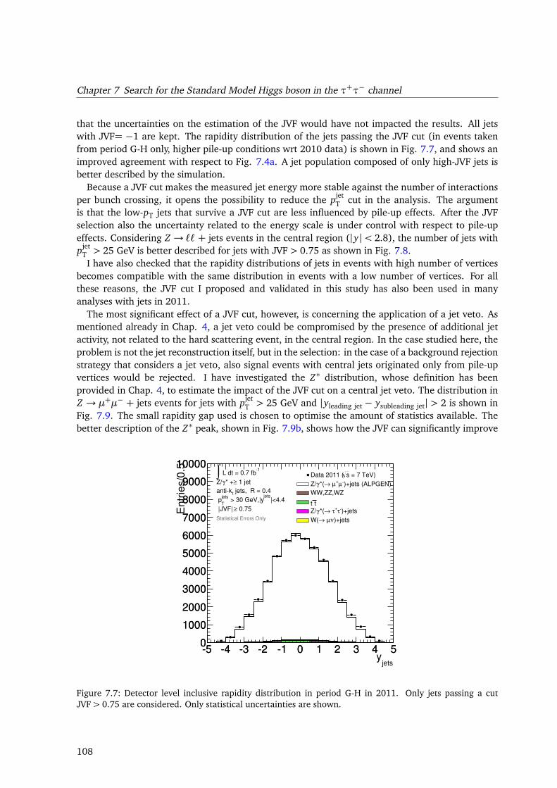
Chapter 7 Search for the Standard Model Higgs boson in the τ+τ− channel
that the uncertainties on the estimation of the JVF would have not impacted the results. All jetswith JVF= −1 are kept. The rapidity distribution of the jets passing the JVF cut (in events takenfrom period G-H only, higher pile-up conditions wrt 2010 data) is shown in Fig. 7.7, and shows animproved agreement with respect to Fig. 7.4a. A jet population composed of only high-JVF jets isbetter described by the simulation.
Because a JVF cut makes the measured jet energy more stable against the number of interactionsper bunch crossing, it opens the possibility to reduce the pjet
T cut in the analysis. The argumentis that the low-pT jets that survive a JVF cut are less influenced by pile-up effects. After the JVFselection also the uncertainty related to the energy scale is under control with respect to pile-upeffects. Considering Z → `` + jets events in the central region (|y| < 2.8), the number of jets withpjet
T > 25 GeV is better described for jets with JVF> 0.75 as shown in Fig. 7.8.I have also checked that the rapidity distributions of jets in events with high number of vertices
becomes compatible with the same distribution in events with a low number of vertices. For allthese reasons, the JVF cut I proposed and validated in this study has also been used in manyanalyses with jets in 2011.
The most significant effect of a JVF cut, however, is concerning the application of a jet veto. Asmentioned already in Chap. 4, a jet veto could be compromised by the presence of additional jetactivity, not related to the hard scattering event, in the central region. In the case studied here, theproblem is not the jet reconstruction itself, but in the selection: in the case of a background rejectionstrategy that considers a jet veto, also signal events with central jets originated only from pile-upvertices would be rejected. I have investigated the Z∗ distribution, whose definition has beenprovided in Chap. 4, to estimate the impact of the JVF cut on a central jet veto. The distribution inZ → µ+µ− + jets events for jets with pjet
T > 25 GeV and |yleading jet − ysubleading jet| > 2 is shown inFig. 7.9. The small rapidity gap used is chosen to optimise the amount of statistics available. Thebetter description of the Z∗ peak, shown in Fig. 7.9b, shows how the JVF can significantly improve
jetsy
5 4 3 2 1 0 1 2 3 4 5
En
trie
s/0
.5
0
1000
2000
3000
4000
5000
6000
7000
8000
9000
10000
5 4 3 2 1 0 1 2 3 4 50
1000
2000
3000
4000
5000
6000
7000
8000
9000
10000 = 7 TeV)sData 2011 (
)+jets (ALPGEN)µ+µ →*(γZ/
WW,ZZ,WZ
tt
)+jetsτ+τ →*(γZ/
)+jetsνµ →W(
1 L dt = 0.7 fb∫
1 jet≥* +γZ/
jets, R = 0.4tantik
|<4.4jets
> 30 GeV,|yjets
T p
0.75≥ |JVF|
Statistical Errors Only
Figure 7.7: Detector level inclusive rapidity distribution in period G-H in 2011. Only jets passing a cutJVF> 0.75 are considered. Only statistical uncertainties are shown.
108
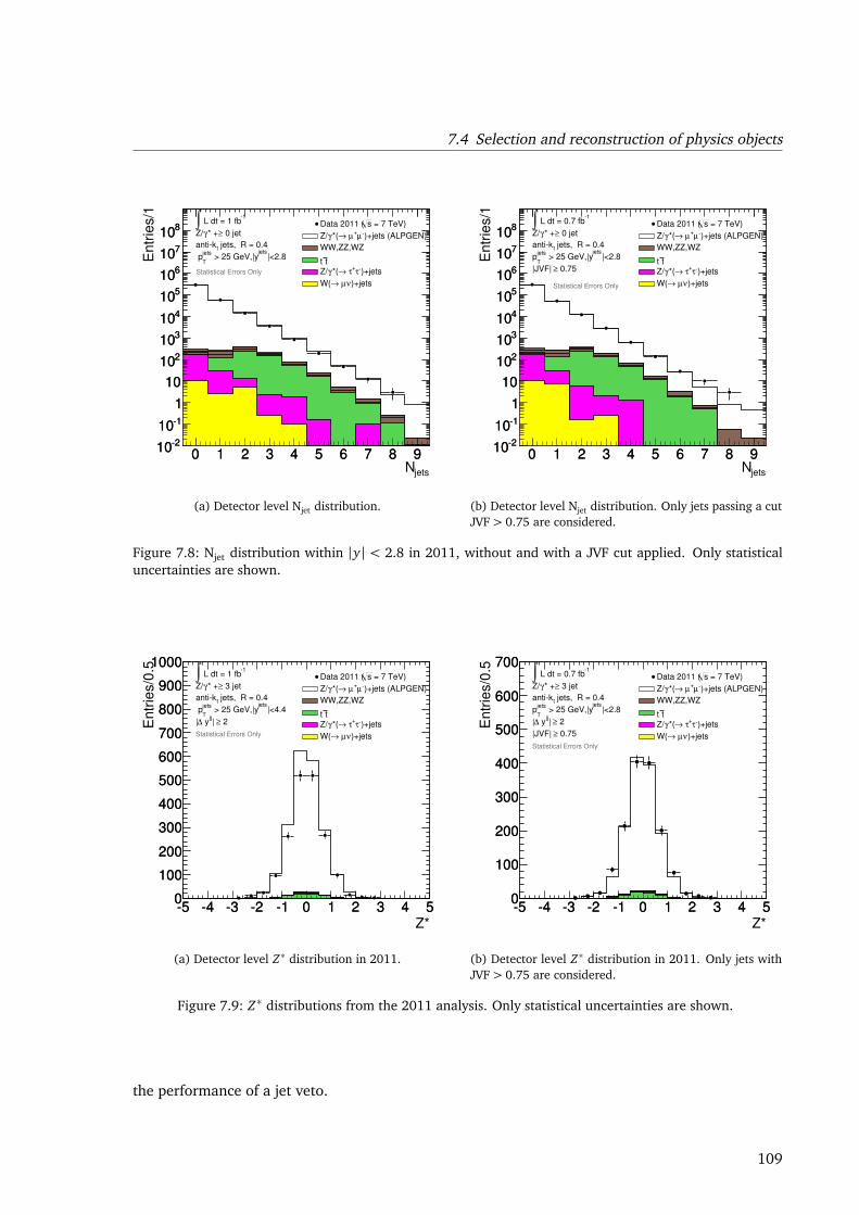
7.4 Selection and reconstruction of physics objects
jetsN0 1 2 3 4 5 6 7 8 9
Entr
ies/1
210
110
1
10
210
310
410
510
610
710
810
0 1 2 3 4 5 6 7 8 9210
110
1
10
210
310
410
510
610
710
810
= 7 TeV)sData 2011 (
)+jets (ALPGEN)µ+µ →*(γZ/
WW,ZZ,WZ
tt
)+jetsτ+τ →*(γZ/
)+jetsνµ →W(
1 L dt = 1 fb∫
0 jet≥* +γZ/
jets, R = 0.4tantik
|<2.8jets
> 25 GeV,|yjets
T p
Statistical Errors Only
(a) Detector level Njet distribution.
jetsN0 1 2 3 4 5 6 7 8 9
Entr
ies/1
210
110
1
10
210
310
410
510
610
710
810
0 1 2 3 4 5 6 7 8 9210
110
1
10
210
310
410
510
610
710
810
= 7 TeV)sData 2011 (
)+jets (ALPGEN)µ+µ →*(γZ/
WW,ZZ,WZ
tt
)+jetsτ+τ →*(γZ/
)+jetsνµ →W(
1 L dt = 0.7 fb∫
0 jet≥* +γZ/
jets, R = 0.4tantik
|<2.8jets
> 25 GeV,|yjets
Tp
0.75≥|JVF|
Statistical Errors Only
(b) Detector level Njet distribution. Only jets passing a cutJVF> 0.75 are considered.
Figure 7.8: Njet distribution within |y| < 2.8 in 2011, without and with a JVF cut applied. Only statisticaluncertainties are shown.
Z*5 4 3 2 1 0 1 2 3 4 5
Entr
ies/0
.5
0
100
200
300
400
500
600
700
800
900
1000
5 4 3 2 1 0 1 2 3 4 50
100
200
300
400
500
600
700
800
900
1000 = 7 TeV)sData 2011 (
)+jets (ALPGEN)µ+µ →*(γZ/
WW,ZZ,WZ
tt
)+jetsτ+τ →*(γZ/
)+jetsνµ →W(
1 L dt = 1 fb∫
3 jet≥* +γZ/
jets, R = 0.4tantik
|<4.4jets
> 25 GeV,|yjets
T p
2≥| jj
y∆|
Statistical Errors Only
(a) Detector level Z∗ distribution in 2011.
Z*5 4 3 2 1 0 1 2 3 4 5
Entr
ies/0
.5
0
100
200
300
400
500
600
700
5 4 3 2 1 0 1 2 3 4 50
100
200
300
400
500
600
700 = 7 TeV)sData 2011 (
)+jets (ALPGEN)µ+µ →*(γZ/
WW,ZZ,WZ
tt
)+jetsτ+τ →*(γZ/
)+jetsνµ →W(
1 L dt = 0.7 fb∫
3 jet≥* +γZ/
jets, R = 0.4tantik
|<2.8jets
> 25 GeV,|yjets
Tp
2≥| jj
y∆|
0.75≥|JVF|
Statistical Errors Only
(b) Detector level Z∗ distribution in 2011. Only jets withJVF> 0.75 are considered.
Figure 7.9: Z∗ distributions from the 2011 analysis. Only statistical uncertainties are shown.
the performance of a jet veto.
109
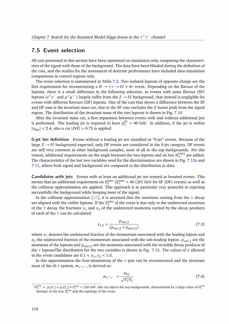
Chapter 7 Search for the Standard Model Higgs boson in the τ+τ− channel
7.5 Event selection
All cuts presented in this section have been optimised on simulation only, comparing the characteri-stics of the signal with those of the background. The data have been blinded during the definition ofthe cuts, and the studies for the assessment of detector performance have included data-simulationcomparisons in control regions only.
The event selection is summarised in Table 7.2. Two isolated leptons of opposite charge are thefirst requirement for reconstructing a H → ττ→ ``+ 4ν event. Depending on the flavour of theleptons, there is a small difference in the following selection, as events with same flavour (SF)leptons (e+e− and µ+µ− ) largely suffer from the Z → `` background, that instead is negligible forevents with different flavours (DF) leptons. One of the cuts that shows a difference between the SFand DF case is the invariant mass cut, that in the SF case excludes the Z boson peak from the signalregion. The distribution of the invariant mass of the two leptons is shown in Fig. 7.10.
After the invariant mass cut, a first separation between events with and without additional jetsis performed. The leading jet is required to have pjet
T > 40 GeV. In addition, if the jet is within|ηdet|< 2.4, also a cut |JVF|> 0.75 is applied.
0-jet bin definition Events without a leading jet are classified as “0-jet” events. Because of thelarge Z → `` background expected, only DF events are considered in the 0-jet category. DF eventsare still very common in other background samples, most of all in the top backgrounds. For thisreason, additional requirements on the angle between the two leptons and on low HLep
T3 are added.
The characteristics of the last two variables used for the discrimination are shown in Fig. 7.12a and7.11, where both signal and background are compared to the distribution in data.
Candidates with jets Events with at least an additional jet are treated as boosted events. Thismeans that an additional requirement on Emiss
T (EmissT > 40 (20) GeV for SF (DF) events) as well as
the collinear approximation are applied. This approach is in particular very powerful in rejectingsuccessfully the background while keeping most of the signal.
In the collinear approximation [59], it is assumed that the neutrinos coming from the τ decayare aligned with the visible leptons. If the Emiss
T of the event is due only to the undetected neutrinosof the τ decay, the fractions x1 and x2 of the undetected momenta carried by the decay productsof each of the τ can be calculated:
x1,2 =pvis1,2
(pvis1,2+ pmis1,2)(7.3)
where x1 denotes the undetected fraction of the momentum associated with the leading lepton andx2 the undetected fraction of the momentum associated with the sub-leading lepton. pvis1,2 are themomenta of the leptons and pmis1,2 are the momenta associated with the invisible decay products ofthe τ leptonsThe distribution for the two variables is shown in Fig. 7.13. The values of x allowedin the event candidates are 0.1< x1, x2 < 1.0.
In this approximation the four-momentum of the τ pair can be reconstructed and the invariantmass of the di-τ system, mτ+τ− , is derived as:
mτ+τ− =m``p
x1 x2(7.4)
3HLepT = pT(`1)+ pT(`2)+ Emiss
T < 120 GeV: this cut rejects the top backgrounds, characterised by a large value of HLepT
because of the true EmissT and the topology of the event.
110
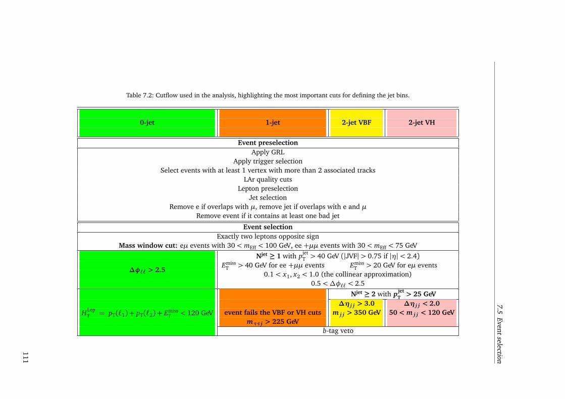
7.5Event
selection
Table 7.2: Cutflow used in the analysis, highlighting the most important cuts for defining the jet bins.
0-jet 1-jet 2-jet VBF 2-jet VH
Event preselectionApply GRL
Apply trigger selectionSelect events with at least 1 vertex with more than 2 associated tracks
LAr quality cutsLepton preselection
Jet selectionRemove e if overlaps with µ, remove jet if overlaps with e and µ
Remove event if it contains at least one bad jet
Event selectionExactly two leptons opposite sign
Mass window cut: eµ events with 30< mEff < 100 GeV, ee +µµ events with 30< mEff < 75 GeV
Njet ≥ 1 with pjetT > 40 GeV (|JVF|> 0.75 if |η|< 2.4)
EmissT > 40 GeV for ee +µµ events Emiss
T > 20 GeV for eµ events0.1< x1, x2 < 1.0 (the collinear approximation)
∆φ`` > 2.5
0.5<∆φ`` < 2.5
Njet ≥ 2 with p jetT > 25 GeV
∆η j j > 3.0 ∆η j j < 2.0event fails the VBF or VH cuts m j j > 350 GeV 50 < m j j < 120 GeV
mττ j > 225 GeVHLep
T = pT(`1) + pT(`2) + EmissT < 120 GeV
b-tag veto
111
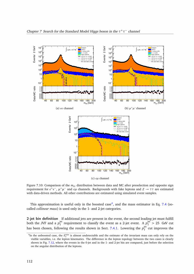
Chapter 7 Search for the Standard Model Higgs boson in the τ+τ− channel
406080100120140160180200
Eve
nts
/ 2
Ge
V
110
1
10
210
310
410
510
610
710 diboson
top(2L)
+jetsµµee,→Z
+jetsττ→Z
Fake Leptons
ll GG→ττ→H×210
ll VBF→ττ→H×3
10
ll VH→ττ→H×3
10
MC stat+fake uncert.
1 Ldt = 4.7 fb∫
[GeV]eem40 60 80 100 120 140 160 180 200D
ata
/MC
ra
tio
0.20.40.60.8
11.21.41.61.8
(a) ee channel 406080100120140160180200E
ve
nts
/ 2
Ge
V
110
1
10
210
310
410
510
610
710diboson
top(2L)
+jetsµµee,→Z
+jetsττ→Z
Fake Leptons
ll GG→ττ→H×210
ll VBF→ττ→H×3
10
ll VH→ττ→H×3
10
MC stat+fake uncert.
1 Ldt = 4.7 fb∫
[GeV]µµm40 60 80 100 120 140 160 180 200D
ata
/MC
ra
tio
0.20.40.60.8
11.21.41.61.8
(b) µ+µ−channel
406080100120140160180200
Eve
nts
/ 2
Ge
V
110
1
10
210
310
410
diboson
top(2L)
+jetsµµee,→Z
+jetsττ→Z
Fake Leptons
ll GG→ττ→H×210
ll VBF→ττ→H×3
10
ll VH→ττ→H×3
10
MC stat+fake uncert.
1 Ldt = 4.7 fb∫
[GeV]µem40 60 80 100 120 140 160 180 200D
ata
/MC
ra
tio
0.20.40.60.8
11.21.41.61.8
(c) eµ channel
Figure 7.10: Comparison of the m`` distribution between data and MC after preselection and opposite signrequirement for e+e−, µ+µ− and eµ channels. Backgrounds with fake leptons and Z → ττ are estimatedwith data-driven methods. All other contributions are estimated using simulated event samples.
This approximation is useful only in the boosted case4, and the mass estimator in Eq. 7.4 (so-called collinear mass) is used only in the 1- and 2-jet categories.
2-jet bin definition If additional jets are present in the event, the second leading jet must fulfillboth the JVF and a pjet
T requirement to classify the event as a 2-jet event. A pjetT > 25 GeV cut
has been chosen, following the results shown in Sect. 7.4.1. Lowering the pjetT cut improves the
4In the unboosted case, the EmissT is almost undetectable and the estimate of the invariant mass can only rely on the
visible variables, i.e. the lepton kinematics. The difference in the lepton topology between the two cases is clearlyshown in Fig. 7.12, where the events in the 0-jet and in the 1- and 2-jet bin are compared, just before the selectionon the angular distribution of the leptons.
112
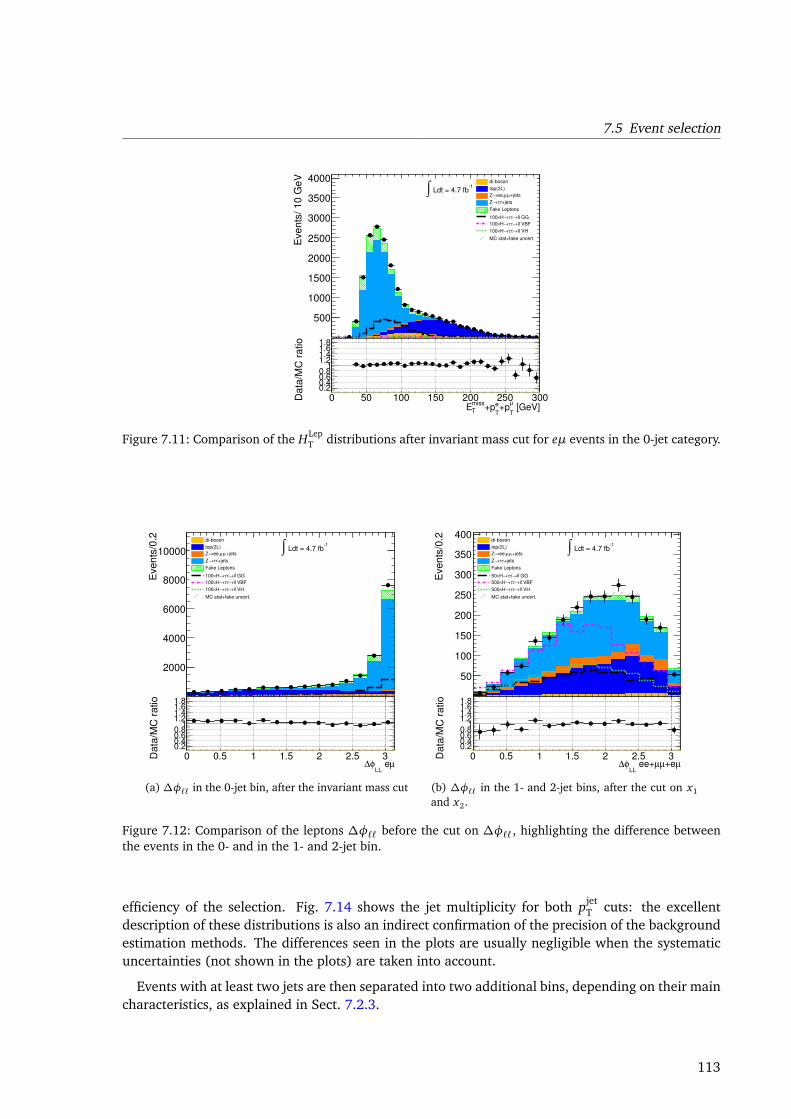
7.5 Event selection
050100150200250300E
ve
nts
/ 1
0 G
eV
500
1000
1500
2000
2500
3000
3500
4000 diboson
top(2L)
+jetsµµee,→Z
+jetsττ→Z
Fake Leptons
ll GG→ττ→H×100
ll VBF→ττ→H×100
ll VH→ττ→H×100
MC stat+fake uncert.
1 Ldt = 4.7 fb∫
[GeV]µ
T+pe
T+p
miss
TE0 50 100 150 200 250 300D
ata
/MC
ra
tio
0.20.40.60.8
11.21.41.61.8
Figure 7.11: Comparison of the HLepT distributions after invariant mass cut for eµ events in the 0-jet category.
00.511.522.53
Eve
nts
/0.2
2000
4000
6000
8000
10000
diboson
top(2L)
+jetsµµee,→Z
+jetsττ→Z
Fake Leptons
ll GG→ττ→H×100
ll VBF→ττ→H×100
ll VH→ττ→H×100
MC stat+fake uncert.
1 Ldt = 4.7 fb∫
µ eLL
φ∆0 0.5 1 1.5 2 2.5 3D
ata
/MC
ra
tio
0.20.40.60.8
11.21.41.61.8
(a) ∆φ`` in the 0-jet bin, after the invariant mass cut 00.511.522.53
Eve
nts
/0.2
50
100
150
200
250
300
350
400diboson
top(2L)
+jetsµµee,→Z
+jetsττ→Z
Fake Leptons
ll GG→ττ→H×50
ll VBF→ττ→H×500
ll VH→ττ→H×500
MC stat+fake uncert.
1 Ldt = 4.7 fb∫
µ+eµµ ee+LL
φ∆0 0.5 1 1.5 2 2.5 3D
ata
/MC
ra
tio
0.20.40.60.8
11.21.41.61.8
(b) ∆φ`` in the 1- and 2-jet bins, after the cut on x1
and x2.
Figure 7.12: Comparison of the leptons ∆φ`` before the cut on ∆φ``, highlighting the difference betweenthe events in the 0- and in the 1- and 2-jet bin.
efficiency of the selection. Fig. 7.14 shows the jet multiplicity for both pjetT cuts: the excellent
description of these distributions is also an indirect confirmation of the precision of the backgroundestimation methods. The differences seen in the plots are usually negligible when the systematicuncertainties (not shown in the plots) are taken into account.
Events with at least two jets are then separated into two additional bins, depending on their maincharacteristics, as explained in Sect. 7.2.3.
113
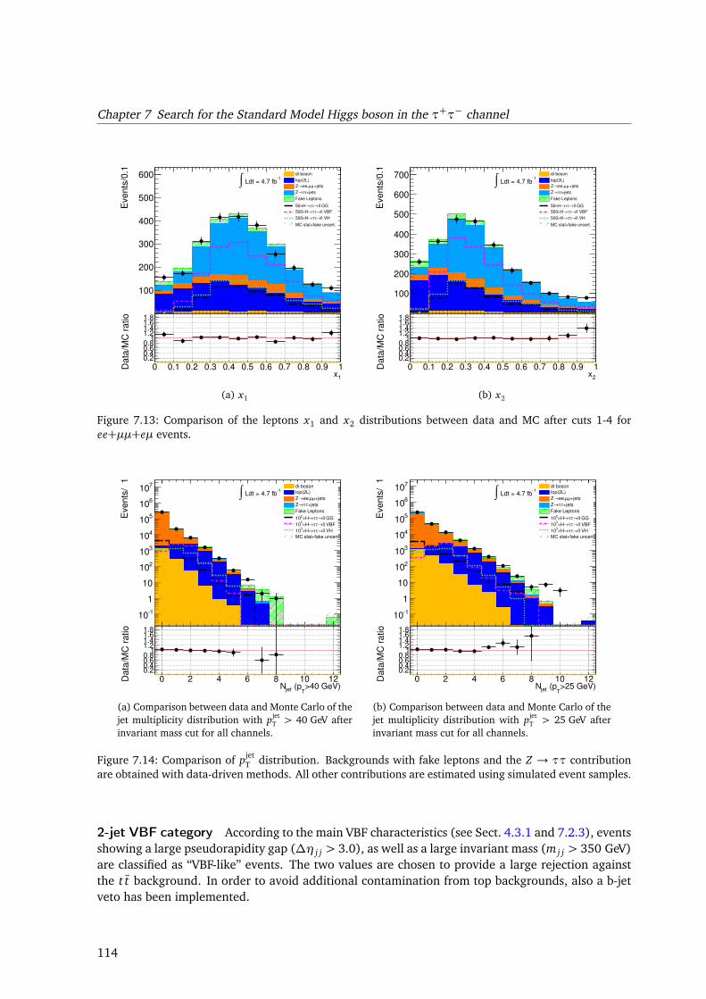
Chapter 7 Search for the Standard Model Higgs boson in the τ+τ− channel
00.10.20.30.40.50.60.70.80.91
Eve
nts
/0.1
100
200
300
400
500
600 diboson
top(2L)
+jetsµµee,→Z
+jetsττ→Z
Fake Leptons
ll GG→ττ→H×50
ll VBF→ττ→H×500
ll VH→ττ→H×500
MC stat+fake uncert.
1 Ldt = 4.7 fb∫
1x0 0.1 0.2 0.3 0.4 0.5 0.6 0.7 0.8 0.9 1D
ata
/MC
ra
tio
0.20.40.60.8
11.21.41.61.8
(a) x1 00.10.20.30.40.50.60.70.80.91E
ve
nts
/0.1
100
200
300
400
500
600
700 diboson
top(2L)
+jetsµµee,→Z
+jetsττ→Z
Fake Leptons
ll GG→ττ→H×50
ll VBF→ττ→H×500
ll VH→ττ→H×500
MC stat+fake uncert.
1 Ldt = 4.7 fb∫
2x0 0.1 0.2 0.3 0.4 0.5 0.6 0.7 0.8 0.9 1D
ata
/MC
ra
tio
0.20.40.60.8
11.21.41.61.8
(b) x2
Figure 7.13: Comparison of the leptons x1 and x2 distributions between data and MC after cuts 1-4 foree+µµ+eµ events.
024681012
Eve
nts
/ 1
110
1
10
210
310
410
510
610
710 diboson
top(2L)
+jetsµµee,→Z
+jetsττ→Z
Fake Leptons
ll GG→ττ→H×210
ll VBF→ττ→H×3
10
ll VH→ττ→H×3
10
MC stat+fake uncert.
1 Ldt = 4.7 fb∫
>40 GeV)T
(pjetN0 2 4 6 8 10 12D
ata
/MC
ra
tio
0.20.40.60.8
11.21.41.61.8
(a) Comparison between data and Monte Carlo of thejet multiplicity distribution with pjet
T > 40 GeV afterinvariant mass cut for all channels. 024681012
Eve
nts
/ 1
110
1
10
210
310
410
510
610
710 diboson
top(2L)
+jetsµµee,→Z
+jetsττ→Z
Fake Leptons
ll GG→ττ→H×210
ll VBF→ττ→H×3
10
ll VH→ττ→H×3
10
MC stat+fake uncert.
1 Ldt = 4.7 fb∫
>25 GeV)T
(pjetN0 2 4 6 8 10 12D
ata
/MC
ra
tio
0.20.40.60.8
11.21.41.61.8
(b) Comparison between data and Monte Carlo of thejet multiplicity distribution with pjet
T > 25 GeV afterinvariant mass cut for all channels.
Figure 7.14: Comparison of pjetT distribution. Backgrounds with fake leptons and the Z → ττ contribution
are obtained with data-driven methods. All other contributions are estimated using simulated event samples.
2-jet VBF category According to the main VBF characteristics (see Sect. 4.3.1 and 7.2.3), eventsshowing a large pseudorapidity gap (∆η j j > 3.0), as well as a large invariant mass (m j j > 350 GeV)are classified as “VBF-like” events. The two values are chosen to provide a large rejection againstthe t t background. In order to avoid additional contamination from top backgrounds, also a b-jetveto has been implemented.
114
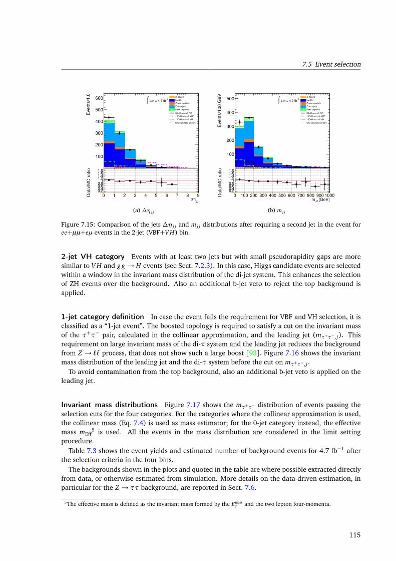
7.5 Event selection
0123456789
Events
/1.0
100
200
300
400
500
600 diboson
top(2L)
+jetsµµee,→Z
+jetsττ→Z
Fake Leptons
ll GG→ττ→H×30
ll VBF→ττ→H×100
ll VH→ττ→H×100
MC stat+fake uncert.
1 Ldt = 4.7 fb∫
JJη∆
0 1 2 3 4 5 6 7 8 9Data
/MC
ratio
0.20.40.60.8
11.21.41.61.8
(a) ∆η j j 01002003004005006007008009001000E
vents
/100 G
eV
100
200
300
400
500diboson
top(2L)
+jetsµµee,→Z
+jetsττ→Z
Fake Leptons
ll GG→ττ→H×30
ll VBF→ττ→H×100
ll VH→ττ→H×100
MC stat+fake uncert.
1 Ldt = 4.7 fb∫
[GeV]JJm0 100 200 300 400 500 600 700 800 900 1000D
ata
/MC
ratio
0.20.40.60.8
11.21.41.61.8
(b) m j j
Figure 7.15: Comparison of the jets ∆η j j and m j j distributions after requiring a second jet in the event foree+µµ+eµ events in the 2-jet (VBF+V H) bin.
2-jet VH category Events with at least two jets but with small pseudorapidity gaps are moresimilar to V H and g g → H events (see Sect. 7.2.3). In this case, Higgs candidate events are selectedwithin a window in the invariant mass distribution of the di-jet system. This enhances the selectionof ZH events over the background. Also an additional b-jet veto to reject the top background isapplied.
1-jet category definition In case the event fails the requirement for VBF and VH selection, it isclassified as a “1-jet event”. The boosted topology is required to satisfy a cut on the invariant massof the τ+τ− pair, calculated in the collinear approximation, and the leading jet (mτ+τ−, j). Thisrequirement on large invariant mass of the di-τ system and the leading jet reduces the backgroundfrom Z → `` process, that does not show such a large boost [93]. Figure 7.16 shows the invariantmass distribution of the leading jet and the di-τ system before the cut on mτ+τ−, j .
To avoid contamination from the top background, also an additional b-jet veto is applied on theleading jet.
Invariant mass distributions Figure 7.17 shows the mτ+τ− distribution of events passing theselection cuts for the four categories. For the categories where the collinear approximation is used,the collinear mass (Eq. 7.4) is used as mass estimator; for the 0-jet category instead, the effectivemass mEff
5 is used. All the events in the mass distribution are considered in the limit settingprocedure.
Table 7.3 shows the event yields and estimated number of background events for 4.7 fb−1 afterthe selection criteria in the four bins.
The backgrounds shown in the plots and quoted in the table are where possible extracted directlyfrom data, or otherwise estimated from simulation. More details on the data-driven estimation, inparticular for the Z → ττ background, are reported in Sect. 7.6.
5The effective mass is defined as the invariant mass formed by the EmissT and the two lepton four-momenta.
115
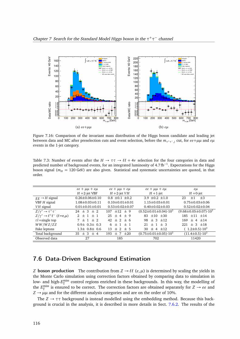
Chapter 7 Search for the Standard Model Higgs boson in the τ+τ− channel
0100200300400500600700800
Events
/ 40 G
eV
20
40
60
80
100
120
140
160diboson
top(2L)
+jetsµµee,→Z
+jetsττ→Z
Fake Leptons
ll GG→ττ→H×50
ll VBF→ττ→H×50
ll VH→ττ→H×50
MC stat+fake uncert.
1 Ldt = 4.7 fb∫
[GeV] jetττm0 100 200 300 400 500 600 700 800D
ata
/MC
ratio
0.20.40.60.8
11.21.41.61.8
(a) ee+µµ 0100200300400500600700800E
vents
/ 40 G
eV
20
40
60
80
100
120
140
160
180
200
220 diboson
top(2L)
+jetsµµee,→Z
+jetsττ→Z
Fake Leptons
ll GG→ττ→H×50
ll VBF→ττ→H×50
ll VH→ττ→H×50
MC stat+fake uncert.
1 Ldt = 4.7 fb∫
[GeV] jetττm0 100 200 300 400 500 600 700 800D
ata
/MC
ratio
0.20.40.60.8
11.21.41.61.8
(b) eµ
Figure 7.16: Comparison of the invariant mass distribution of the Higgs boson candidate and leading jetbetween data and MC after preselection cuts and event selection, before the mτ+τ−, j cut, for ee+µµ and eµevents in the 1-jet category.
Table 7.3: Number of events after the H → ττ → `` + 4ν selection for the four categories in data andpredicted number of background events, for an integrated luminosity of 4.7 fb−1. Expectations for the Higgsboson signal (mH = 120 GeV) are also given. Statistical and systematic uncertainties are quoted, in thatorder.
ee + µµ + eµ ee + µµ + eµ ee + µµ + eµ eµH +2-jet VBF H +2-jet V H H +1-jet H +0-jet
g g → H signal 0.26±0.06±0.10 0.8 ±0.1 ±0.2 3.9 ±0.2 ±1.0 23 ±1 ±3VBF H signal 1.08±0.03±0.11 0.10±0.01±0.01 1.15±0.03±0.01 0.75±0.03±0.06V H signal 0.01±0.01±0.01 0.53±0.02±0.07 0.40±0.02±0.03 0.52±0.02±0.04Z/γ∗→ τ+τ− 24 ± 3 ± 2 107 ±12 ± 9 (0.52±0.01±0.04)·103 (9.68±0.05±0.07)·103
Z/γ∗→ `+`− (`=e,µ) 2 ± 1 ± 1 25 ± 4 ± 9 83 ±10 ±30 185 ±11 ±14t t+single top 7 ± 1 ± 2 42 ± 2 ± 6 98 ± 3 ±12 169 ± 4 ±14WW/W Z/Z Z 0.9± 0.3± 0.3 6 ± 1 ± 1 21 ± 1 ± 3 221 ± 3 ±18Fake leptons 1.3± 0.8± 0.6 13 ± 2 ± 5 30 ± 4 ±12 ( 1.2±0.5)·103
Total background 35 ± 3 ± 4 193 ± 7 ±20 (0.75±0.01±0.05)·103 (11.4±0.5)·103
Observed data 27 185 702 11420
7.6 Data-Driven Background Estimation
Z boson production The contribution from Z → `` (e,µ) is determined by scaling the yields inthe Monte Carlo simulation using correction factors obtained by comparing data to simulation inlow- and high-Emiss
T control regions enriched in these backgrounds. In this way, the modelling ofthe Emiss
T is ensured to be correct. The correction factors are obtained separately for Z → ee andZ → µµ and for the different analysis categories and are on the order of 10%.
The Z → ττ background is instead modelled using the embedding method. Because this back-ground is crucial in the analysis, it is described in more details in Sect. 7.6.2. The results of the
116
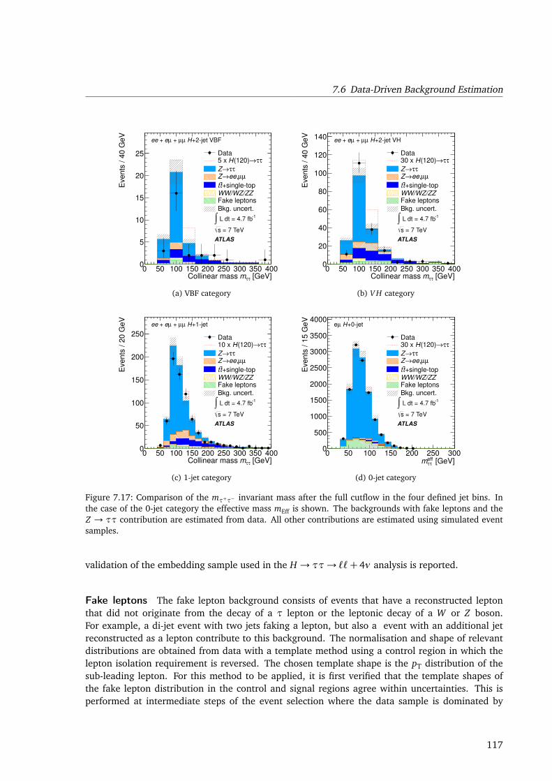
7.6 Data-Driven Background Estimation
[GeV]ττmCollinear mass 0 50 100 150 200 250 300 350 400
Eve
nts
/ 4
0 G
eV
0
5
10
15
20
25 Dataττ→(120)H5 x
ττ→Z
µµ,ee→Z
+singletoptt
WW/WZ/ZZ
Fake leptons
Bkg. uncert.
ATLAS
= 7 TeVs
1 L dt = 4.7 fb∫
+2jet VBFH µµ + µe + ee
(a) VBF category
[GeV]ττmCollinear mass 0 50 100 150 200 250 300 350 400
Eve
nts
/ 4
0 G
eV
0
20
40
60
80
100
120
140
Dataττ→(120)H30 x
ττ→Z
µµ,ee→Z
+singletoptt
WW/WZ/ZZ
Fake leptons
Bkg. uncert.
ATLAS
= 7 TeVs
1 L dt = 4.7 fb∫
+2jet VHH µµ + µe + ee
(b) V H category
[GeV]ττmCollinear mass 0 50 100 150 200 250 300 350 400
Eve
nts
/ 2
0 G
eV
0
50
100
150
200
250 Dataττ→(120)H10 x
ττ→Z
µµ,ee→Z
+singletoptt
WW/WZ/ZZ
Fake leptons
Bkg. uncert.
ATLAS
= 7 TeVs
1 L dt = 4.7 fb∫
+1jetH µµ + µe + ee
(c) 1-jet category
[GeV]effττm
0 50 100 150 200 250 300
Eve
nts
/ 1
5 G
eV
0
500
1000
1500
2000
2500
3000
3500
4000
Dataττ→(120)H30 x
ττ→Z
µµ,ee→Z
+singletoptt
WW/WZ/ZZ
Fake leptons
Bkg. uncert.
ATLAS
= 7 TeVs
1 L dt = 4.7 fb∫
+0jetH µe
(d) 0-jet category
Figure 7.17: Comparison of the mτ+τ− invariant mass after the full cutflow in the four defined jet bins. Inthe case of the 0-jet category the effective mass mEff is shown. The backgrounds with fake leptons and theZ → ττ contribution are estimated from data. All other contributions are estimated using simulated eventsamples.
validation of the embedding sample used in the H → ττ→ ``+ 4ν analysis is reported.
Fake leptons The fake lepton background consists of events that have a reconstructed leptonthat did not originate from the decay of a τ lepton or the leptonic decay of a W or Z boson.For example, a di-jet event with two jets faking a lepton, but also a event with an additional jetreconstructed as a lepton contribute to this background. The normalisation and shape of relevantdistributions are obtained from data with a template method using a control region in which thelepton isolation requirement is reversed. The chosen template shape is the pT distribution of thesub-leading lepton. For this method to be applied, it is first verified that the template shapes ofthe fake lepton distribution in the control and signal regions agree within uncertainties. This isperformed at intermediate steps of the event selection where the data sample is dominated by
117
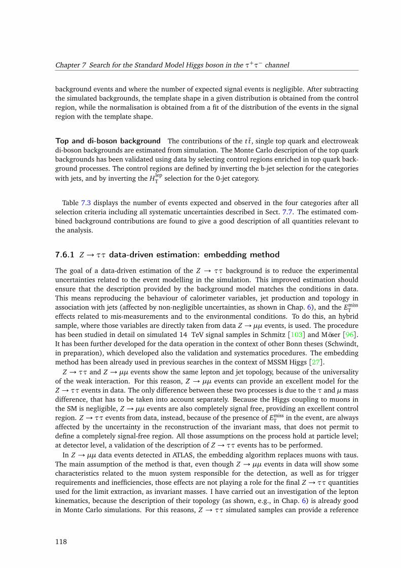
Chapter 7 Search for the Standard Model Higgs boson in the τ+τ− channel
background events and where the number of expected signal events is negligible. After subtractingthe simulated backgrounds, the template shape in a given distribution is obtained from the controlregion, while the normalisation is obtained from a fit of the distribution of the events in the signalregion with the template shape.
Top and di-boson background The contributions of the t t, single top quark and electroweakdi-boson backgrounds are estimated from simulation. The Monte Carlo description of the top quarkbackgrounds has been validated using data by selecting control regions enriched in top quark back-ground processes. The control regions are defined by inverting the b-jet selection for the categorieswith jets, and by inverting the H lep
T selection for the 0-jet category.
Table 7.3 displays the number of events expected and observed in the four categories after allselection criteria including all systematic uncertainties described in Sect. 7.7. The estimated com-bined background contributions are found to give a good description of all quantities relevant tothe analysis.
7.6.1 Z → ττ data-driven estimation: embedding method
The goal of a data-driven estimation of the Z → ττ background is to reduce the experimentaluncertainties related to the event modelling in the simulation. This improved estimation shouldensure that the description provided by the background model matches the conditions in data.This means reproducing the behaviour of calorimeter variables, jet production and topology inassociation with jets (affected by non-negligible uncertainties, as shown in Chap. 6), and the Emiss
Teffects related to mis-measurements and to the environmental conditions. To do this, an hybridsample, where those variables are directly taken from data Z → µµ events, is used. The procedurehas been studied in detail on simulated 14 TeV signal samples in Schmitz [103] and Möser [96].It has been further developed for the data operation in the context of other Bonn theses (Schwindt,in preparation), which developed also the validation and systematics procedures. The embeddingmethod has been already used in previous searches in the context of MSSM Higgs [27].
Z → ττ and Z → µµ events show the same lepton and jet topology, because of the universalityof the weak interaction. For this reason, Z → µµ events can provide an excellent model for theZ → ττ events in data. The only difference between these two processes is due to the τ and µmassdifference, that has to be taken into account separately. Because the Higgs coupling to muons inthe SM is negligible, Z → µµ events are also completely signal free, providing an excellent controlregion. Z → ττ events from data, instead, because of the presence of Emiss
T in the event, are alwaysaffected by the uncertainty in the reconstruction of the invariant mass, that does not permit todefine a completely signal-free region. All those assumptions on the process hold at particle level;at detector level, a validation of the description of Z → ττ events has to be performed.
In Z → µµ data events detected in ATLAS, the embedding algorithm replaces muons with taus.The main assumption of the method is that, even though Z → µµ events in data will show somecharacteristics related to the muon system responsible for the detection, as well as for triggerrequirements and inefficiencies, those effects are not playing a role for the final Z → ττ quantitiesused for the limit extraction, as invariant masses. I have carried out an investigation of the leptonkinematics, because the description of their topology (as shown, e.g., in Chap. 6) is already goodin Monte Carlo simulations. For this reasons, Z → ττ simulated samples can provide a reference
118
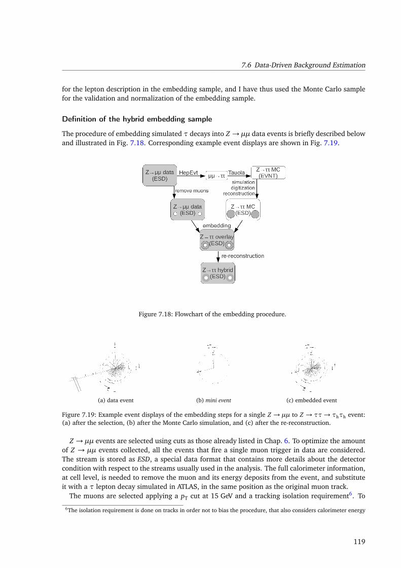
7.6 Data-Driven Background Estimation
for the lepton description in the embedding sample, and I have thus used the Monte Carlo samplefor the validation and normalization of the embedding sample.
Definition of the hybrid embedding sample
The procedure of embedding simulated τ decays into Z → µµ data events is briefly described belowand illustrated in Fig. 7.18. Corresponding example event displays are shown in Fig. 7.19.
Figure 7.18: Flowchart of the embedding procedure.
(a) data event (b) mini event (c) embedded event
Figure 7.19: Example event displays of the embedding steps for a single Z → µµ to Z → ττ→ τhτh event:(a) after the selection, (b) after the Monte Carlo simulation, and (c) after the re-reconstruction.
Z → µµ events are selected using cuts as those already listed in Chap. 6. To optimize the amountof Z → µµ events collected, all the events that fire a single muon trigger in data are considered.The stream is stored as ESD, a special data format that contains more details about the detectorcondition with respect to the streams usually used in the analysis. The full calorimeter information,at cell level, is needed to remove the muon and its energy deposits from the event, and substituteit with a τ lepton decay simulated in ATLAS, in the same position as the original muon track.
The muons are selected applying a pT cut at 15 GeV and a tracking isolation requirement6. To
6The isolation requirement is done on tracks in order not to bias the procedure, that also considers calorimeter energy
119
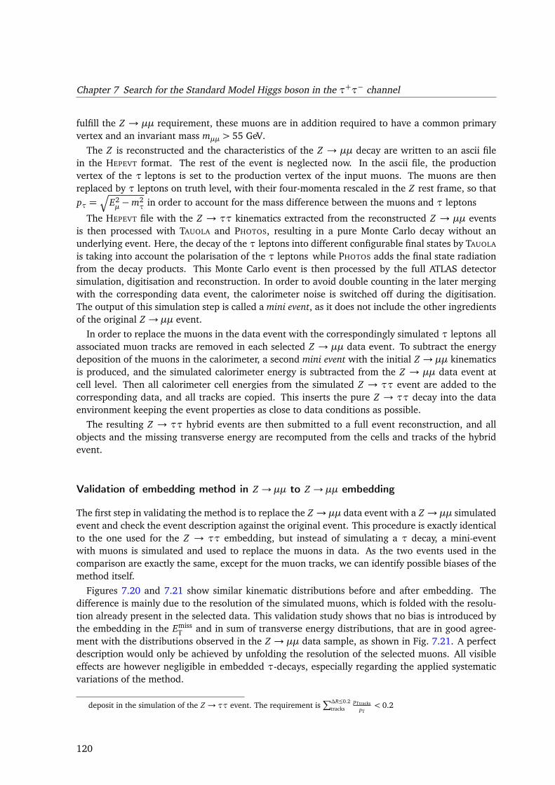
Chapter 7 Search for the Standard Model Higgs boson in the τ+τ− channel
fulfill the Z → µµ requirement, these muons are in addition required to have a common primaryvertex and an invariant mass mµµ > 55 GeV.
The Z is reconstructed and the characteristics of the Z → µµ decay are written to an ascii filein the HEPEVT format. The rest of the event is neglected now. In the ascii file, the productionvertex of the τ leptons is set to the production vertex of the input muons. The muons are thenreplaced by τ leptons on truth level, with their four-momenta rescaled in the Z rest frame, so thatpτ =
Æ
E2µ−m2
τ in order to account for the mass difference between the muons and τ leptons
The HEPEVT file with the Z → ττ kinematics extracted from the reconstructed Z → µµ eventsis then processed with TAUOLA and PHOTOS, resulting in a pure Monte Carlo decay without anunderlying event. Here, the decay of the τ leptons into different configurable final states by TAUOLA
is taking into account the polarisation of the τ leptons while PHOTOS adds the final state radiationfrom the decay products. This Monte Carlo event is then processed by the full ATLAS detectorsimulation, digitisation and reconstruction. In order to avoid double counting in the later mergingwith the corresponding data event, the calorimeter noise is switched off during the digitisation.The output of this simulation step is called a mini event, as it does not include the other ingredientsof the original Z → µµ event.
In order to replace the muons in the data event with the correspondingly simulated τ leptons allassociated muon tracks are removed in each selected Z → µµ data event. To subtract the energydeposition of the muons in the calorimeter, a second mini event with the initial Z → µµ kinematicsis produced, and the simulated calorimeter energy is subtracted from the Z → µµ data event atcell level. Then all calorimeter cell energies from the simulated Z → ττ event are added to thecorresponding data, and all tracks are copied. This inserts the pure Z → ττ decay into the dataenvironment keeping the event properties as close to data conditions as possible.
The resulting Z → ττ hybrid events are then submitted to a full event reconstruction, and allobjects and the missing transverse energy are recomputed from the cells and tracks of the hybridevent.
Validation of embedding method in Z → µµ to Z → µµ embedding
The first step in validating the method is to replace the Z → µµ data event with a Z → µµ simulatedevent and check the event description against the original event. This procedure is exactly identicalto the one used for the Z → ττ embedding, but instead of simulating a τ decay, a mini-eventwith muons is simulated and used to replace the muons in data. As the two events used in thecomparison are exactly the same, except for the muon tracks, we can identify possible biases of themethod itself.
Figures 7.20 and 7.21 show similar kinematic distributions before and after embedding. Thedifference is mainly due to the resolution of the simulated muons, which is folded with the resolu-tion already present in the selected data. This validation study shows that no bias is introduced bythe embedding in the Emiss
T and in sum of transverse energy distributions, that are in good agree-ment with the distributions observed in the Z → µµ data sample, as shown in Fig. 7.21. A perfectdescription would only be achieved by unfolding the resolution of the selected muons. All visibleeffects are however negligible in embedded τ-decays, especially regarding the applied systematicvariations of the method.
deposit in the simulation of the Z → ττ event. The requirement is∑∆R≤0.2
trackspTtracks
pT< 0.2
120
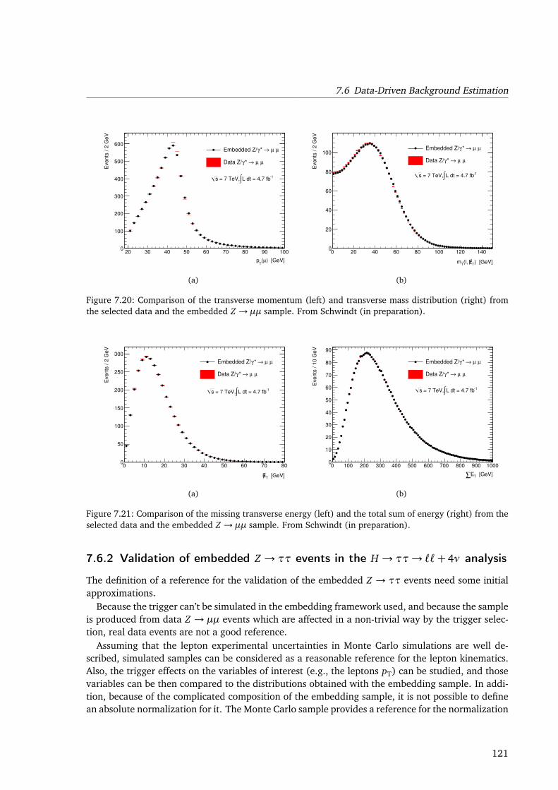
7.6 Data-Driven Background Estimation
) [GeV]µ(T
p
20 30 40 50 60 70 80 90 100
Eve
nts
/ 2
Ge
V
0
100
200
300
400
500
600µ µ →* γEmbedded Z/
µ µ →* γData Z/
1L dt = 4.7 fb∫ = 7 TeV, s
(a)
) [GeV]T
E(l, T
m
0 20 40 60 80 100 120 140
Eve
nts
/ 2
Ge
V
0
20
40
60
80
100µ µ →* γEmbedded Z/
µ µ →* γData Z/
1L dt = 4.7 fb∫ = 7 TeV, s
(b)
Figure 7.20: Comparison of the transverse momentum (left) and transverse mass distribution (right) fromthe selected data and the embedded Z → µµ sample. From Schwindt (in preparation).
[GeV]T
E
0 10 20 30 40 50 60 70 80
Eve
nts
/ 2
Ge
V
0
50
100
150
200
250
300
µ µ →* γEmbedded Z/
µ µ →* γData Z/
1L dt = 4.7 fb∫ = 7 TeV, s
(a)
[GeV]TE∑
0 100 200 300 400 500 600 700 800 900 1000
Eve
nts
/ 1
0 G
eV
0
10
20
30
40
50
60
70
80
90
µ µ →* γEmbedded Z/
µ µ →* γData Z/
1L dt = 4.7 fb∫ = 7 TeV, s
(b)
Figure 7.21: Comparison of the missing transverse energy (left) and the total sum of energy (right) from theselected data and the embedded Z → µµ sample. From Schwindt (in preparation).
7.6.2 Validation of embedded Z → ττ events in the H → ττ→ ``+ 4ν analysis
The definition of a reference for the validation of the embedded Z → ττ events need some initialapproximations.
Because the trigger can’t be simulated in the embedding framework used, and because the sampleis produced from data Z → µµ events which are affected in a non-trivial way by the trigger selec-tion, real data events are not a good reference.
Assuming that the lepton experimental uncertainties in Monte Carlo simulations are well de-scribed, simulated samples can be considered as a reasonable reference for the lepton kinematics.Also, the trigger effects on the variables of interest (e.g., the leptons pT) can be studied, and thosevariables can be then compared to the distributions obtained with the embedding sample. In addi-tion, because of the complicated composition of the embedding sample, it is not possible to definean absolute normalization for it. The Monte Carlo sample provides a reference for the normalization
121
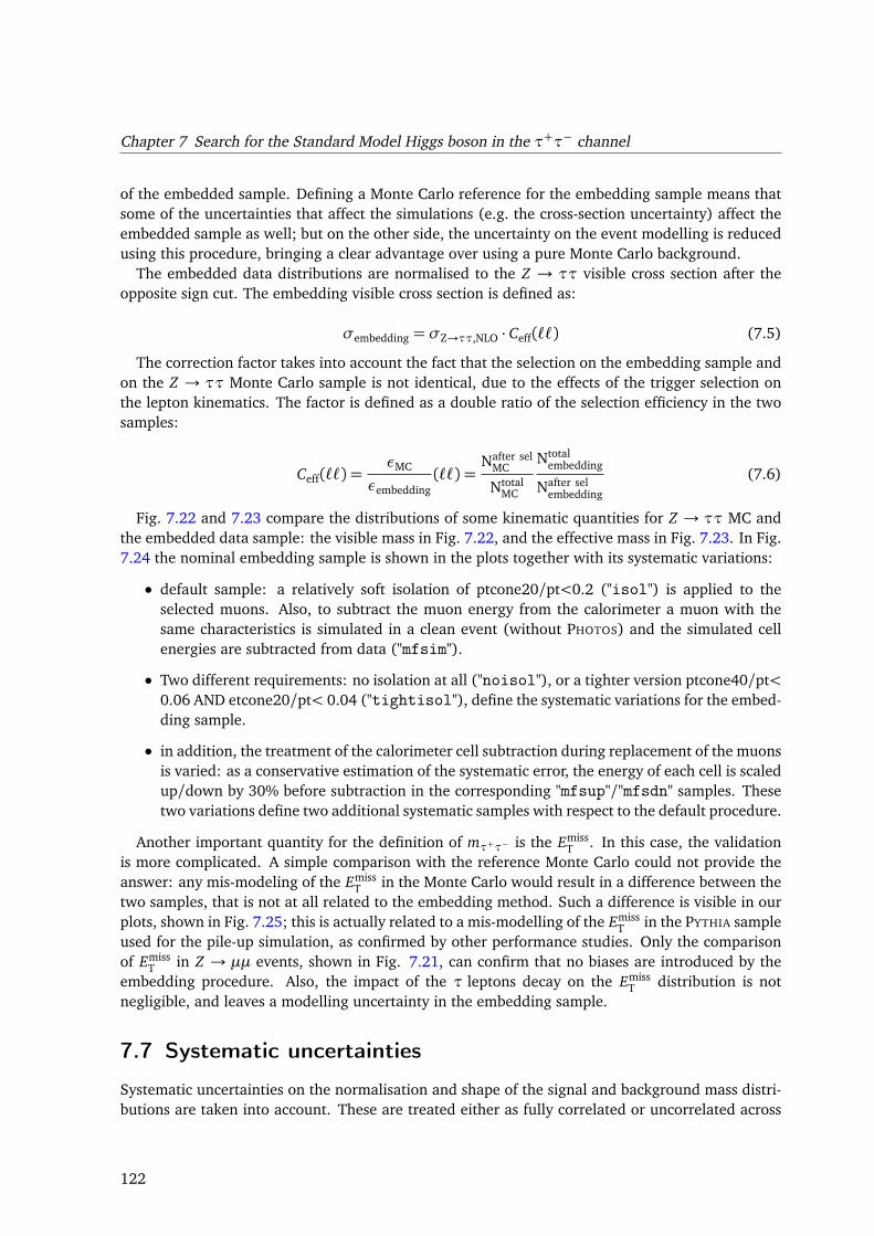
Chapter 7 Search for the Standard Model Higgs boson in the τ+τ− channel
of the embedded sample. Defining a Monte Carlo reference for the embedding sample means thatsome of the uncertainties that affect the simulations (e.g. the cross-section uncertainty) affect theembedded sample as well; but on the other side, the uncertainty on the event modelling is reducedusing this procedure, bringing a clear advantage over using a pure Monte Carlo background.
The embedded data distributions are normalised to the Z → ττ visible cross section after theopposite sign cut. The embedding visible cross section is defined as:
σembedding = σZ→ττ,NLO · Ceff(``) (7.5)
The correction factor takes into account the fact that the selection on the embedding sample andon the Z → ττ Monte Carlo sample is not identical, due to the effects of the trigger selection onthe lepton kinematics. The factor is defined as a double ratio of the selection efficiency in the twosamples:
Ceff(``) =εMC
εembedding(``) =
Nafter selMC
NtotalMC
Ntotalembedding
Nafter selembedding
(7.6)
Fig. 7.22 and 7.23 compare the distributions of some kinematic quantities for Z → ττ MC andthe embedded data sample: the visible mass in Fig. 7.22, and the effective mass in Fig. 7.23. In Fig.7.24 the nominal embedding sample is shown in the plots together with its systematic variations:
• default sample: a relatively soft isolation of ptcone20/pt<0.2 ("isol") is applied to theselected muons. Also, to subtract the muon energy from the calorimeter a muon with thesame characteristics is simulated in a clean event (without PHOTOS) and the simulated cellenergies are subtracted from data ("mfsim").
• Two different requirements: no isolation at all ("noisol"), or a tighter version ptcone40/pt<0.06 AND etcone20/pt< 0.04 ("tightisol"), define the systematic variations for the embed-ding sample.
• in addition, the treatment of the calorimeter cell subtraction during replacement of the muonsis varied: as a conservative estimation of the systematic error, the energy of each cell is scaledup/down by 30% before subtraction in the corresponding "mfsup"/"mfsdn" samples. Thesetwo variations define two additional systematic samples with respect to the default procedure.
Another important quantity for the definition of mτ+τ− is the EmissT . In this case, the validation
is more complicated. A simple comparison with the reference Monte Carlo could not provide theanswer: any mis-modeling of the Emiss
T in the Monte Carlo would result in a difference between thetwo samples, that is not at all related to the embedding method. Such a difference is visible in ourplots, shown in Fig. 7.25; this is actually related to a mis-modelling of the Emiss
T in the PYTHIA sampleused for the pile-up simulation, as confirmed by other performance studies. Only the comparisonof Emiss
T in Z → µµ events, shown in Fig. 7.21, can confirm that no biases are introduced by theembedding procedure. Also, the impact of the τ leptons decay on the Emiss
T distribution is notnegligible, and leaves a modelling uncertainty in the embedding sample.
7.7 Systematic uncertainties
Systematic uncertainties on the normalisation and shape of the signal and background mass distri-butions are taken into account. These are treated either as fully correlated or uncorrelated across
122
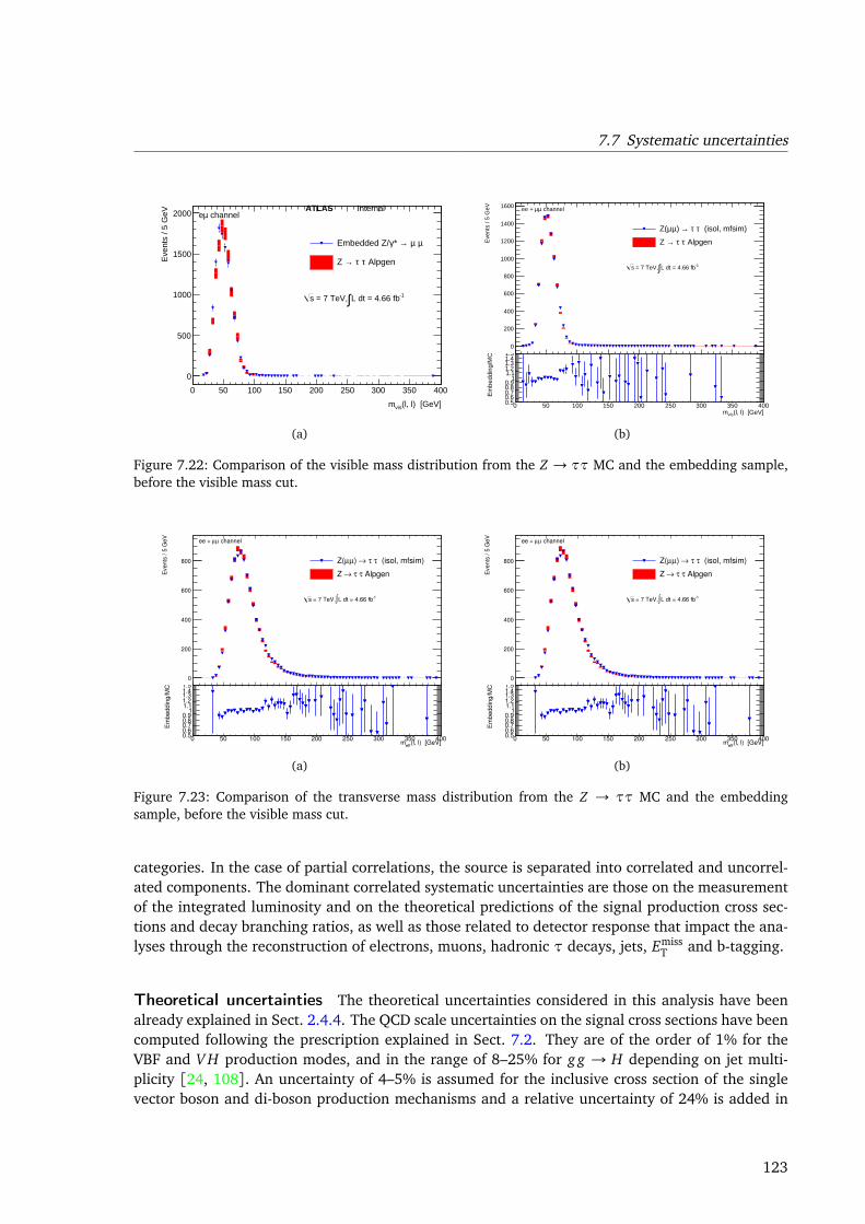
7.7 Systematic uncertainties
(l, l) [GeV]vism
0 50 100 150 200 250 300 350 400
Eve
nts
/ 5 G
eV
0
500
1000
1500
2000
µ µ →* γEmbedded Z/
Alpgenτ τ →Z
channelµe
-1L dt = 4.66 fb∫ = 7 TeV, s
ATLAS Internal
(a)
(l, l) [GeV]vism
0 50 100 150 200 250 300 350 400
Eve
nts
/ 5 G
eV
0
200
400
600
800
1000
1200
1400
1600
(isol, mfsim)τ τ →) µµZ(
Alpgenτ τ →Z
channelµµee +
-1L dt = 4.66 fb∫ = 7 TeV, s
(l, l) [GeV]vism0 50 100 150 200 250 300 350 400
Em
bedd
ing/
MC
0.50.60.70.80.9
11.11.21.31.41.5
(b)
Figure 7.22: Comparison of the visible mass distribution from the Z → ττ MC and the embedding sample,before the visible mass cut.
Events
/ 5
GeV
0
200
400
600
800 (isol, mfsim)τ τ →) µµZ(
Alpgenτ τ →Z
channelµµee +
1L dt = 4.66 fb∫ = 7 TeV, s
(l, l) [GeV]eff
m0 50 100 150 200 250 300 350 400
Em
beddin
g/M
C
0.50.60.70.80.9
11.11.21.31.41.5
(a)
Events
/ 5
GeV
0
200
400
600
800 (isol, mfsim)τ τ →) µµZ(
Alpgenτ τ →Z
channelµµee +
1L dt = 4.66 fb∫ = 7 TeV, s
(l, l) [GeV]eff
m0 50 100 150 200 250 300 350 400
Em
beddin
g/M
C
0.50.60.70.80.9
11.11.21.31.41.5
(b)
Figure 7.23: Comparison of the transverse mass distribution from the Z → ττ MC and the embeddingsample, before the visible mass cut.
categories. In the case of partial correlations, the source is separated into correlated and uncorrel-ated components. The dominant correlated systematic uncertainties are those on the measurementof the integrated luminosity and on the theoretical predictions of the signal production cross sec-tions and decay branching ratios, as well as those related to detector response that impact the ana-lyses through the reconstruction of electrons, muons, hadronic τ decays, jets, Emiss
T and b-tagging.
Theoretical uncertainties The theoretical uncertainties considered in this analysis have beenalready explained in Sect. 2.4.4. The QCD scale uncertainties on the signal cross sections have beencomputed following the prescription explained in Sect. 7.2. They are of the order of 1% for theVBF and V H production modes, and in the range of 8–25% for g g → H depending on jet multi-plicity [24, 108]. An uncertainty of 4–5% is assumed for the inclusive cross section of the singlevector boson and di-boson production mechanisms and a relative uncertainty of 24% is added in
123
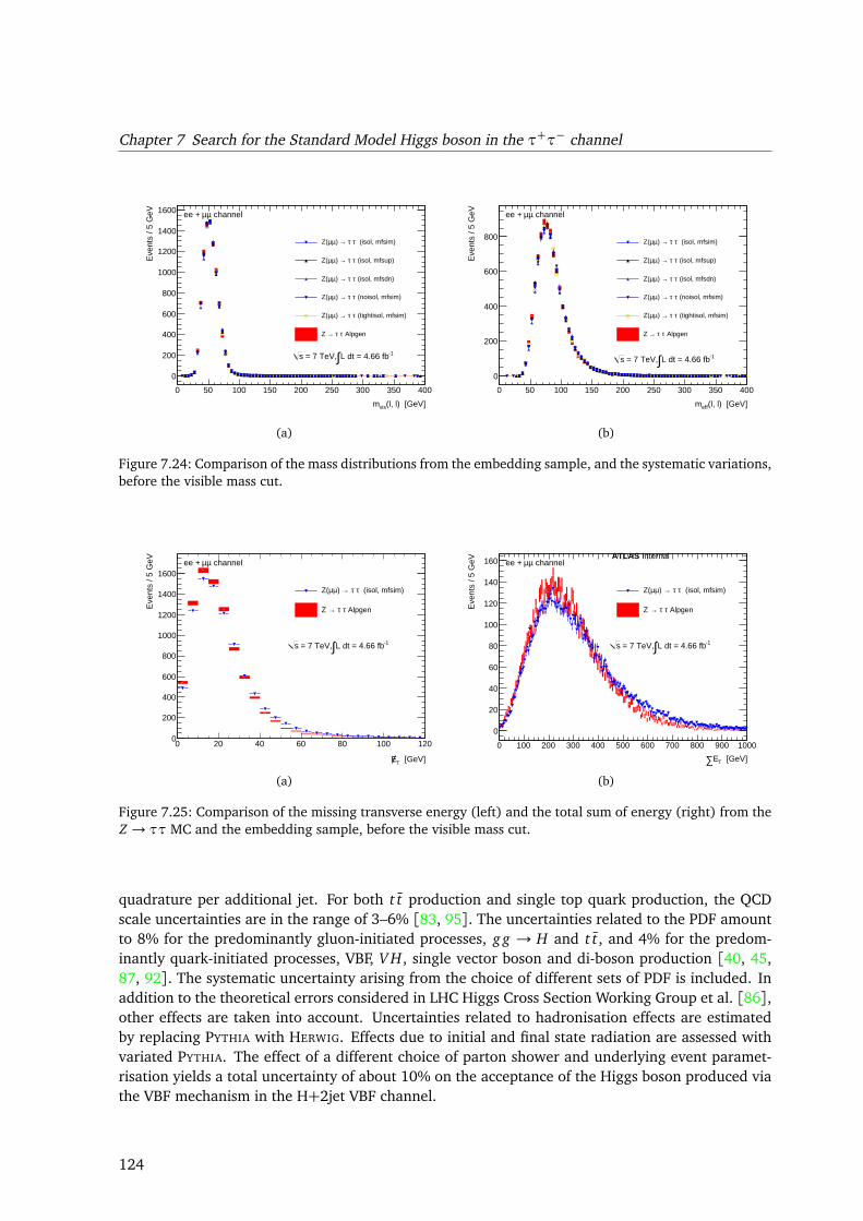
Chapter 7 Search for the Standard Model Higgs boson in the τ+τ− channel
(l, l) [GeV]vism
0 50 100 150 200 250 300 350 400
Eve
nts
/ 5 G
eV
0
200
400
600
800
1000
1200
1400
1600
(isol, mfsim)τ τ →) µµZ(
(isol, mfsup)τ τ →) µµZ(
(isol, mfsdn)τ τ →) µµZ(
(noisol, mfsim)τ τ →) µµZ(
(tightisol, mfsim)τ τ →) µµZ(
Alpgenτ τ →Z
channelµµee +
-1L dt = 4.66 fb∫ = 7 TeV, s
(a)
(l, l) [GeV]effm
0 50 100 150 200 250 300 350 400
Eve
nts
/ 5 G
eV
0
200
400
600
800 (isol, mfsim)τ τ →) µµZ(
(isol, mfsup)τ τ →) µµZ(
(isol, mfsdn)τ τ →) µµZ(
(noisol, mfsim)τ τ →) µµZ(
(tightisol, mfsim)τ τ →) µµZ(
Alpgenτ τ →Z
channelµµee +
-1L dt = 4.66 fb∫ = 7 TeV, s
(b)
Figure 7.24: Comparison of the mass distributions from the embedding sample, and the systematic variations,before the visible mass cut.
[GeV]TE
0 20 40 60 80 100 120
Eve
nts
/ 5 G
eV
0
200
400
600
800
1000
1200
1400
1600
(isol, mfsim)τ τ →) µµZ(
Alpgenτ τ →Z
channelµµee +
-1L dt = 4.66 fb∫ = 7 TeV, s
(a)
[GeV]TE∑0 100 200 300 400 500 600 700 800 900 1000
Eve
nts
/ 5 G
eV
0
20
40
60
80
100
120
140
160
(isol, mfsim)τ τ →) µµZ(
Alpgenτ τ →Z
channelµµee +
-1L dt = 4.66 fb∫ = 7 TeV, s
ATLAS Internal
(b)
Figure 7.25: Comparison of the missing transverse energy (left) and the total sum of energy (right) from theZ → ττ MC and the embedding sample, before the visible mass cut.
quadrature per additional jet. For both t t production and single top quark production, the QCDscale uncertainties are in the range of 3–6% [83, 95]. The uncertainties related to the PDF amountto 8% for the predominantly gluon-initiated processes, g g → H and t t, and 4% for the predom-inantly quark-initiated processes, VBF, V H, single vector boson and di-boson production [40, 45,87, 92]. The systematic uncertainty arising from the choice of different sets of PDF is included. Inaddition to the theoretical errors considered in LHC Higgs Cross Section Working Group et al. [86],other effects are taken into account. Uncertainties related to hadronisation effects are estimatedby replacing PYTHIA with HERWIG. Effects due to initial and final state radiation are assessed withvariated PYTHIA. The effect of a different choice of parton shower and underlying event paramet-risation yields a total uncertainty of about 10% on the acceptance of the Higgs boson produced viathe VBF mechanism in the H+2jet VBF channel.
124
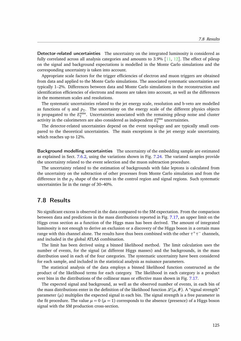
7.8 Results
Detector-related uncertainties The uncertainty on the integrated luminosity is considered asfully correlated across all analysis categories and amounts to 3.9% [11, 12]. The effect of pileupon the signal and background expectations is modelled in the Monte Carlo simulations and thecorresponding uncertainty is taken into account.
Appropriate scale factors for the trigger efficiencies of electron and muon triggers are obtainedfrom data and applied to the Monte Carlo simulations. The associated systematic uncertainties aretypically 1–2%. Differences between data and Monte Carlo simulations in the reconstruction andidentification efficiencies of electrons and muons are taken into account, as well as the differencesin the momentum scales and resolutions.
The systematic uncertainties related to the jet energy scale, resolution and b-veto are modelledas functions of η and pT. The uncertainty on the energy scale of the different physics objectsis propagated to the Emiss
T . Uncertainties associated with the remaining pileup noise and clusteractivity in the calorimeters are also considered as independent Emiss
T uncertainties.The detector-related uncertainties depend on the event topology and are typically small com-
pared to the theoretical uncertainties. The main exceptions is the jet energy scale uncertainty,which reaches up to 12%.
Background modelling uncertainties The uncertainty of the embedding sample are estimatedas explained in Sect. 7.6.2, using the variations shown in Fig. 7.24. The variated samples providethe uncertainty related to the event selection and the muon subtraction procedure.
The uncertainty related to the estimation of backgrounds with fake leptons is calculated fromthe uncertainty on the subtraction of other processes from Monte Carlo simulation and from thedifference in the pT shape of the events in the control region and signal regions. Such systematicuncertainties lie in the range of 30–40%.
7.8 Results
No significant excess is observed in the data compared to the SM expectation. From the comparisonbetween data and predictions in the mass distributions reported in Fig. 7.17, an upper limit on theHiggs cross section as a function of the Higgs mass has been derived. The amount of integratedluminosity is not enough to derive an exclusion or a discovery of the Higgs boson in a certain massrange with this channel alone. The results have thus been combined with the other τ+τ− channels,and included in the global ATLAS combination.
The limit has been derived using a binned likelihood method. The limit calculation uses thenumber of events, for the signal (at different Higgs masses) and the backgrounds, in the massdistribution used in each of the four categories. The systematic uncertainty have been consideredfor each sample, and included in the statistical analysis as nuisance parameters.
The statistical analysis of the data employs a binned likelihood function constructed as theproduct of the likelihood terms for each category. The likelihood in each category is a productover bins in the distributions of the collinear mass or effective mass shown in Fig. 7.17.
The expected signal and background, as well as the observed number of events, in each bin ofthe mass distributions enter in the definition of the likelihood functionL (µ,θ ). A “signal strength”parameter (µ) multiplies the expected signal in each bin. The signal strength is a free parameter inthe fit procedure. The value µ= 0 (µ= 1) corresponds to the absence (presence) of a Higgs bosonsignal with the SM production cross-section.
125
Chapter 7 Search for the Standard Model Higgs boson in the τ+τ− channel
Signal and background predictions (s and b) depend on systematic uncertainties that are para-metrised by nuisance parameters θ , which in turn are constrained using Gaussian functions. Thecorrelation of the systematic uncertainties across categories are taken into account:
L (µ,θ) =∏
bin j
Poisson(N j|µ(s j) + b j)∏
θ
Gaussian(θ |0,1). (7.7)
The expected signal and background event counts in each bin are functions of θ . The paramet-risation is chosen such that the rates in each channel are log-normally distributed for a normallydistributed θ .
The test statistic qµ is defined as:
qµ =−2 ln
L (µ, θµ)/L (µ, θ )
, (7.8)
where µ and θ refer to the global maximum of the likelihood (with the constraint 0 ≤ µ ≤ µ)and θµ corresponds to the conditional maximum likelihood of θ for a given µ. This test statistic isused to compute exclusion limits following the modified frequentist method known as CLs [100].The asymptotic approximation [55] is used to evaluate the Gaussian probability density functionsrather than performing pseudo-experiments and the procedure has been validated using ensembletests.
The profile likelihood formalism used in this statistical analysis incorporates the information onthe observed and expected number of events, nuisance parameters, probability density functionsand parameters of interest. The statistical significance of an excess is evaluated in terms of the sameprofile likelihood test statistic. The expected sensitivity and the ±1,2σ bands are obtained for thebackground expectation in the absence of a Standard Model Higgs boson signal. The consistencywith the background-only hypothesis is quantified using the p-value, the probability that the teststatistic of a background-only experiment fluctuates to at least the observed one.
No significant excess is observed in the data compared to the SM expectation. Exclusion limitsat the 95% confidence level, normalised to the Standard Model cross section times the branchingratio of H → τ+τ− (σSM), are set as a function of the Higgs boson mass. The limit plot is shown inFig. 7.26.
The expected limits vary between 7 and 17 times the predicted Standard Model cross sectiontimes branching ratio for the mass range 100− 150 GeV. The most sensitive categories is the VBFcategory, that is limited by statistics in the 2011 analysis. The observed limits are in the rangebetween 5 and 15 times the predicted Standard Model cross section times branching ratio for thesame mass range. No significant deviation from the background-only hypothesis is observed.
7.9 Outlook
This analysis brought a large improvement in the H → ττ analysis via the consistent treatment ofall production and decay processes considered, and by using their characteristics to enhance thesensitivity to the signal. Selecting events according to the jet multiplicity in the final state increasesthe rejection power with respect to a simple, inclusive analysis.
The analysis performed in 2011 is still limited by statistics in its most sensitive bin, the 2-jet VBFcategory. The possibility to use a central jet veto has not been used yet, because of the low statisticsin the bin before the eventual veto; with higher statistics, it would provide an even better separationof signal from background. The JVF, used in the jet selection, ensures a reliable operation of the
126
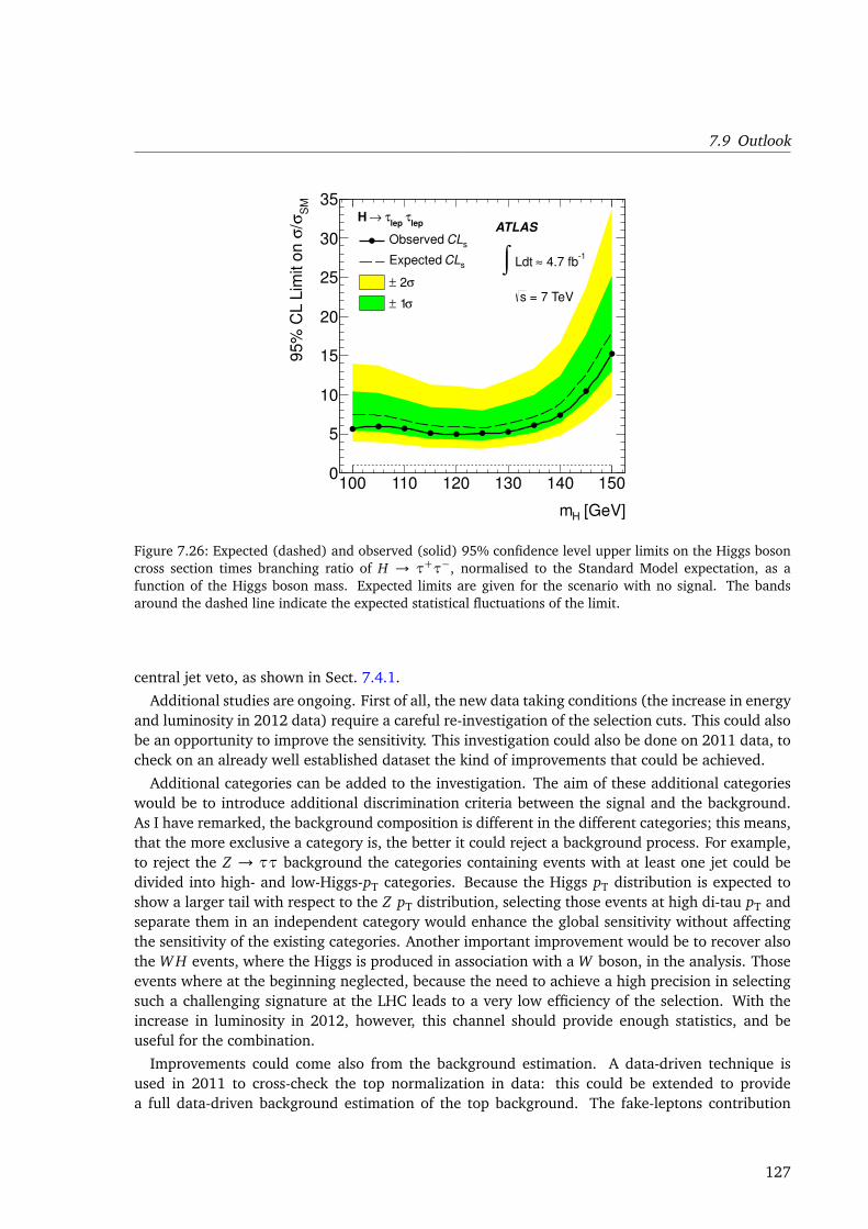
7.9 Outlook
[GeV]Hm
100 110 120 130 140 150
SM
σ/σ
95%
CL L
imit o
n
0
5
10
15
20
25
30
35
lepτ
lepτ →H
sCLObserved
sCLExpected
σ 2±
σ 1±
ATLAS
1 4.7 fb≈ Ldt ∫
= 7 TeVs
Figure 7.26: Expected (dashed) and observed (solid) 95% confidence level upper limits on the Higgs bosoncross section times branching ratio of H → τ+τ−, normalised to the Standard Model expectation, as afunction of the Higgs boson mass. Expected limits are given for the scenario with no signal. The bandsaround the dashed line indicate the expected statistical fluctuations of the limit.
central jet veto, as shown in Sect. 7.4.1.
Additional studies are ongoing. First of all, the new data taking conditions (the increase in energyand luminosity in 2012 data) require a careful re-investigation of the selection cuts. This could alsobe an opportunity to improve the sensitivity. This investigation could also be done on 2011 data, tocheck on an already well established dataset the kind of improvements that could be achieved.
Additional categories can be added to the investigation. The aim of these additional categorieswould be to introduce additional discrimination criteria between the signal and the background.As I have remarked, the background composition is different in the different categories; this means,that the more exclusive a category is, the better it could reject a background process. For example,to reject the Z → ττ background the categories containing events with at least one jet could bedivided into high- and low-Higgs-pT categories. Because the Higgs pT distribution is expected toshow a larger tail with respect to the Z pT distribution, selecting those events at high di-tau pT andseparate them in an independent category would enhance the global sensitivity without affectingthe sensitivity of the existing categories. Another important improvement would be to recover alsothe W H events, where the Higgs is produced in association with a W boson, in the analysis. Thoseevents where at the beginning neglected, because the need to achieve a high precision in selectingsuch a challenging signature at the LHC leads to a very low efficiency of the selection. With theincrease in luminosity in 2012, however, this channel should provide enough statistics, and beuseful for the combination.
Improvements could come also from the background estimation. A data-driven technique isused in 2011 to cross-check the top normalization in data: this could be extended to providea full data-driven background estimation of the top background. The fake-leptons contribution
127
Chapter 7 Search for the Standard Model Higgs boson in the τ+τ− channel
is already estimated data-driven, and an improvement of this technique is needed to reduce itssystematic uncertainty, that dominates the background uncertainty. For the Z → `` background,it is already under control; further studies of the Z → `` + jets background could anyway lowerthe uncertainty on the normalization, by providing more precise predictions, and this would alsoimpact the normalization of the Z → ττ background. For the embedding procedure, developmentand improvements will also need to take into account the changes in the data-taking conditions,that affect the sample selection.
Finally, an improvement planned in ATLAS is to unify the mass definitions used in the analy-sis. The H → ττ → τh` analysis uses already a sophisticated mass estimator, the Missing MassCalculator [58]. Such mass estimator achieves a better mass resolution with respect to the massestimators used in the H → ττ→ ``+4ν analysis, and, as already mentioned, the mass resolutionis crucial for the extraction of the signal. Several studies in ATLAS are ongoing, related to the useand calibration of such estimator, and a non-negligible improvement is expected in 2012 also fromthe implementation of this estimator.
128
Chapter 8
Outlook
An observed excess of events, corresponding to the hypothesis of a new particle with mass 126±0.4(stat.) ±0.4 (syst.), has now (July 2012) been reported by the ATLAS collaboration [21]. Alsothe CMS collaboration at LHC has reported a similar result [110]. The results in the H → γγ,H → Z Z (∗)→ ```` and H →WW ∗→ `ν`ν channels are compatible with a Higgs boson hypothesis,the observed deviations from the SM expectations being still small to be statistically significant.However, many measurements are needed in order to assess the nature of this particle; and furtherdevelopments, starting from the results presented in this work, will be very important in this effort.
H → ττ studies in 2012 The hypothesis of a Higgs boson could not be verified without checkingthat this particles decays into fermions. With respect to earlier studies [57], that predicted a visibleH → ττ at higher integrated luminosity and only in the VBF channel, the 2011 ATLAS analysishas shown that the H → ττ analysis can provide an input to the Higgs combination already witha low integrated luminosity. The increase in luminosity will definitely provide the possibility toimprove the limit and approach the σ/σSM level, with the possibility of setting direct limits fromthis channel alone. Also, the possible observation of an excess of events could be expected.
Observing or not an excess would be a fundamental input to the current Higgs studies. The τ+τ−
channel is the cleanest channel that provides a Higgs decay to fermions: observing it is fundamentalboth in the study of the Higgs characteristics in general, as well as for understanding the Yukawacoupling of the Higgs to fermions, that is included “ad-hoc” in the SM to reproduce the particlemasses. For this reason, the H → ττ analysis is expected to play a very important role within theHiggs analyses. Not only the SM Higgs analysis will be affected: many BSM scenarios predict adifferent coupling of the Higgs to the tau lepton. In general, measuring any possible deviation fromthe SM expectation of the Higgs decay rate would be the only way at the LHC to get informationsabout the total Higgs width around mH = 126 GeV, and on any possible new physics process thatcould influence the observed values.
Neglecting or not carefully estimating the uncertainties would yield, in the case of negativesearch results, to an overestimate of the excluded regions of the parameter space. In case of aHiggs signal these uncertainties are crucial to perform a reliable and accurate determination ofmH and of the Higgs boson couplings. As already mentioned in the thesis, both experimental andtheoretical uncertainties need to be carefully understood and estimated to ensure the success of theanalysis.
Development in modelling and uncertainties Experimental uncertainties have been reducedduring the first two LHC runs, thanks to a precise estimate of the performance. Still, some of theseuncertainties are dominating the analyses, and limit the possibility for additional improvements.One of such examples is the Z → `` + jets analysis, where the main limit is now the jet energy scaleuncertainty. The first results, documented here, from the Z → `` + jets cross section measurement
129
Chapter 8 Outlook
showed that the current understanding of the process, provided by matrix element generators in-terfaced with a parton shower generator is satisfactory; but deviations have been observed, mostlyin the di-jet quantities shown in Fig. 6.13, that are at the moment under investigation, both in theATLAS collaboration and by the authors of the Monte Carlo generators.
Another experimental improvement in the JES calibration has been brought in 2011 by the im-plementation of the in-situ calibrations. To keep detector effects and physics effects well separated,and to have a well defined reference, the jets measured in data have been calibrated using cor-rection factors derived from the data-Monte Carlo comparison. In this way, the calibration is stillbased on Monte Carlo, but the combination of the corrections coming from the in-situ techniquesshould better address several uncertainties of the older calibrations (e.g. the quark-gluon effects inthe EM+JES, and the jet-level corrections in the LCW calibration). The improvements in 2011 havebeen already very large, with the largest uncertainty (the uncertainty at low pjet
T in the forwardregion) dropping to 6% from the previous 12%. But to get at the level of the other experimentaluncertainties, the aim is to bring it down to 1%, and for this the current strategy needs still to beimproved. Because of the large impact of the Monte Carlo predictions on the ATLAS jet energyscale determination, any improvement in the Monte Carlo modelling will propagate to the JEScalibration and uncertainty.
One of the top priorities of the experiment, however, will be the understanding of the experi-mental conditions. In this thesis, the impact of pile-up effects on the measurement has been shownin several examples; and, with the LHC increasing in instantaneous luminosity, the need to updateboth the performance studies and the Monte Carlo simulations is crucial. In 2012, with a higherenergy and higher pile-up conditions, the results have already been successful.
Developments and the long-term goals The theoretical modelling will still be one of the toppriorities in the Higgs searches. The Z → `` + jets analysis has shown that the theoretical modelsavailable for that process are satisfactory; but the Z → `` + jets process is a process whose per-turbative series converges quite well, in contrast with the Higgs production channels, in particularg g → H[86]. The ATLAS strategy has carefully addressed this point, and several discussions havebeen ongoing between ATLAS and CMS experimentalists, and theorists. Any improvement or op-timized selection of the phase space needs to be cross-checked with the theory uncertainty, in ordernot to fall into ill-defined regions. This effort will be even more important if the results from thedifferent decay channels will be combined to extract the Higgs couplings: for such an analysis, agood knowledge of the production processes is needed. In the past, the need for such a precisionhas brought the collaborations to neglect some cases, as for example the g g → H production inthe H → ττ channel. A full combination of the LHC results will be an outstanding results for thescientific community, showing how the understanding of both the theoretical predictions and theexperimental conditions have been successful at the LHC.
130
Bibliography
[1] [Online]. Available: https://twiki.cern.ch/twiki/bin/view/AtlasPublic.
[2] 2010. [Online]. Available: atlas.ch.
[3] A. Ribon et al. (2010). Status of Geant4 hadronic physics for the simulation of LHC exper-iments at the start of the LHC physics program.
[4] ATLAS: technical proposal for a general-purpose pp experiment at the Large Hadron Colliderat CERN, ser. LHC Tech. Proposal. Geneva: CERN, 2010.
[5] G. Aad et al., ‘ATLAS Calorimeter Response to Single Isolated Hadrons and Estimation ofthe Calorimeter Jet Scale Uncertainty’, CERN, Geneva, Tech. Rep. ATLAS-CONF-2011-028,2011.
[6] —, ‘Charged particle multiplicities in pp interactions for track pT > 100 MeV atp
s =0.9 and 7 TeV measured with the ATLAS detector at the LHC’, CERN, Geneva, Tech. Rep.ATLAS-CONF-2010-046, 2010.
[7] —, ‘Commissioning of the ATLAS high-performance b-tagging algorithms in the 7 TeV col-lision data’, CERN, Geneva, Tech. Rep. ATLAS-CONF-2011-102, 2011.
[8] —, ‘Electron performance measurements with the ATLAS detector using the 2010 LHCproton-proton collision data’, Oct. 2011. eprint: 1110.3174v2. [Online]. Available: http://arxiv.org/abs/1110.3174v2.
[9] —, Expected Performance of the ATLAS Experiment, Detector, Trigger and Physics. Geneva,2008.
[10] —, ‘Jet energy measurement with the ATLAS detector in proton-proton collisions atp
s =7 TeV’, 2011. arXiv:1112.6426 [hep-ex].
[11] —, ‘Luminosity Determination in pp Collisions atp
(s) = 7TeV using the ATLAS Detector in2011’, CERN, Geneva, Tech. Rep. ATLAS-CONF-2011-116, 2011.
[12] —, ‘Luminosity determination in pp collisions atp
s = 7 TeV using the ATLAS detector atthe LHC’, The European Physical Journal C - Particles and Fields, vol. 71, no. 4, p. 1630,2011. DOI: 10.1140/epjc/s10052-011-1630-5.
[13] —, ‘Measurement of the Mistag Rate with 5 fb1 of Data Collected by the ATLAS Detector’,CERN, Geneva, Tech. Rep. ATLAS-CONF-2012-040, 2012.
[14] —, ‘Measurement of the W -> lnu and Z/gamma* -> ll production cross sections in proton-proton collisions at sqrt(s) = 7 TeV with the ATLAS detector’, JHEP, vol. 12, p. 060, 2010.DOI: 10.1007/JHEP12(2010)060. arXiv:1010.2130 [hep-ex].
[15] —, ‘Measurement of the b-tag Efficiency in a Sample of Jets Containing Muons with 5 fb1 ofData from the ATLAS Detector’, CERN, Geneva, Tech. Rep. ATLAS-CONF-2012-043, 2012.
[16] —, ‘Measurement of the inclusive W+- and Z/gamma cross sections in the electron andmuon decay channels in pp collisions at sqrt(s) = 7 TeV with the ATLAS detector’, 2011.arXiv:1109.5141 [hep-ex].
131
Bibliography
[17] —, ‘Measurement of the production cross section for Z/γ∗ in association with jets in ppcollisions at
ps = 7 TeV with the ATLAS detector’, Phys. Rev. D, vol. 85, p. 032 009, 3 2012.
DOI: 10.1103/PhysRevD.85.032009. [Online]. Available: http://link.aps.org/doi/10.1103/PhysRevD.85.032009.
[18] —, ‘Measurement of underlying event characteristics using charged particles in pp colli-sions at
ps = 900 GeV and 7 TeV with the ATLAS detector’, Phys. Rev. D, vol. 83, p. 112 001,
11 2011. DOI: 10.1103/PhysRevD.83.112001. [Online]. Available: http://link.aps.org/doi/10.1103/PhysRevD.83.112001.
[19] —, ‘Muon Reconstruction Performance’, CERN, Geneva, Tech. Rep. ATLAS-CONF-2010-064,2010.
[20] —, ‘Muon reconstruction efficiency in reprocessed 2010 LHC proton-proton collision datarecorded with the ATLAS detector’, CERN, Geneva, Tech. Rep. ATLAS-CONF-2011-063,2011.
[21] —, ‘Observation of a new particle in the search for the Standard Model Higgs boson withthe ATLAS detector at the LHC’, Jul. 2012. eprint: 1207.7214v1. [Online]. Available:http://arxiv.org/abs/1207.7214v1.
[22] —, ‘Performance of missing transverse momentum reconstruction in proton-proton colli-sions at 7 TeV with ATLAS’, Eur. Phys. J., vol. C72, p. 1844, 2012. DOI: 10.1140/epjc/s10052-011-1844-6. arXiv:1108.5602 [hep-ex].
[23] —, ‘Performance of the ATLAS Trigger System in 2010’, Eur. Phys. J., vol. C72, p. 1849,2012. DOI: 10.1140/epjc/s10052-011-1849-1. arXiv:1110.1530 [hep-ex].
[24] —, ‘Procedure for the LHC Higgs boson search combination in summer 2011’, CERN,Geneva, Tech. Rep. ATL-PHYS-PUB-2011-011, 2011.
[25] —, ‘Response of isolated particles identified using resonances in proton-proton collisions atsqr ts=7 TeV with the ATLAS detector’, CERN, Geneva, Tech. Rep. ATLAS-CONF-2011-019,2011.
[26] —, ‘Response of the ATLAS calorimeters to single isolated hadrons produced in protonproton collisions at a center of mass energy of sqrts = 900 GeV’, CERN, Geneva, Tech. Rep.ATLAS-CONF-2010-017, 2010.
[27] —, ‘Search for neutral MSSM Higgs bosons decaying to τ+τ− pairs in proton-proton col-lisions at sqrt(s) = 7 TeV with the ATLAS detector’, Phys. Lett., vol. B705, pp. 174–192,2011. DOI: 10.1016/j.physletb.2011.10.001. arXiv:1107.5003 [hep-ex].
[28] —, ‘Search for the Standard Model Higgs boson in the H to tau+ tau− decay mode inp
(s) = 7TeV pp collisions with ATLAS’, Jun. 2012. eprint: 1206.5971v1. [Online]. Avail-able: http://arxiv.org/abs/1206.5971v1.
[29] —, ‘Search for the Standard Model Higgs boson in the decay mode H → τ+τ− → ll +4 neutrinos in Association with jets in Proton-Proton Collisions at
p
(s) = 7 TeV with theATLAS detector’, CERN, Geneva, Tech. Rep. ATLAS-CONF-2011-133, 2011.
[30] —, ‘Study of Jet Shapes in Inclusive Jet Production in pp Collisions at sqrt(s) = 7 TeV usingthe ATLAS Detector’, Phys. Rev., vol. D83, p. 052 003, 2011. DOI: 10.1103/PhysRevD.83.052003. arXiv:1101.0070 [hep-ex].
132
Bibliography
[31] —, ‘The ATLAS Experiment at the CERN Large Hadron Collider’, JINST, vol. 3, no. 08,S08003, August 2008.
[32] —, ‘The ATLAS Simulation Infrastructure’, Eur. Phys. J., vol. C70, pp. 823–874, 2010. DOI:10.1140/epjc/s10052-010-1429-9. arXiv:1005.4568 [physics.ins-det].
[33] T. Adye, ‘Unfolding algorithms and tests using roounfold’, May 2011. eprint: 1105.1160v1.[Online]. Available: http://arxiv.org/abs/1105.1160v1.
[34] S. Agostinelli et al., ‘Geant4 a simulation toolkit’, Nuclear Instruments and Methods in Phys-ics Research Section A: Accelerators, Spectrometers, Detectors and Associated Equipment, vol.506, no. 3, pp. 250 –303, 2003, ISSN: 0168-9002. DOI: 10.1016/S0168- 9002(03)01368-8. [Online]. Available: http://www.sciencedirect.com/science/article/pii/S0168900203013688.
[35] N. Amelin", ‘Transverse flow and collectivity in ultrarelativistic heavy-ion collisions’, Phys-ical Review Letters, vol. 67, no. 12, pp. 1523–1526, 1991. DOI: 10.1103/PhysRevLett.67.1523.
[36] N. Amelin et al., ‘Collectivity in ultra-relativistic heavy ion collisions’, Nuclear Physics A,vol. 544, no. 1â“2, pp. 463 –466, 1992, ISSN: 0375-9474. DOI: 10.1016/0375-9474(92)90598-E. [Online]. Available: http://www.sciencedirect.com/science/article/pii/037594749290598E.
[37] AthenaROOTAccess, documentation available from the ATLAS Protected wiki. [Online].Available: twiki.cern.ch/twiki/bin/view/AtlasProtected/AthenaROOTAccess.
[38] M. Baak et al., ‘Updated Status of the Global Electroweak Fit and Constraints on NewPhysics’, 2011. arXiv:1107.0975 [hep-ph].
[39] M. Bahr et al., ‘Herwig++ Physics and Manual’, Eur.Phys.J., vol. C58, pp. 639–707, 2008.DOI: 10.1140/epjc/s10052-008-0798-9. arXiv:0803.0883 [hep-ph].
[40] R. D. Ball et al., ‘Impact of heavy quark masses on parton distributions and LHC phenomen-ology’, Nucl.Phys., vol. B849, pp. 296–363, 2011. DOI: 10.1016/j.nuclphysb.2011.03.021. arXiv:1101.1300 [hep-ph].
[41] C. Berger et al., ‘Vector Boson + Jets with BlackHat and Sherpa’, Nucl.Phys.Proc.Suppl., vol.205-206, pp. 92–97, 2010. DOI: 10.1016/j.nuclphysbps.2010.08.025. arXiv:1005.3728 [hep-ph].
[42] J. Beringer et al., ‘Review of particle physics’, Physical Review D, vol. 86, no. 1, 2012. DOI:10.1103/PhysRevD.86.010001.
[43] H. Bertini, ‘Intranuclear-Cascade Calculation of the Secondary Nucleon Spectra from Nucleon-Nucleus Interactions in the Energy Range 340 to 2900 MeV and Comparisons with Exper-iment’, Physical Review, vol. 188, no. 4, pp. 1711–1730, 1969. DOI: 10.1103/PhysRev.188.1711.
[44] P. Bolzoni et al., ‘Higgs production via vector-boson fusion at NNLO in QCD’, Mar. 2010.eprint: 1003.4451v2. [Online]. Available: http://arxiv.org/abs/1003.4451v2.
[45] M. Botje et al., ‘The PDF4LHC working group interim recommendations’, 2011. arXiv:1101.0538 [hep-ph].
133
Bibliography
[46] L. Bravina, ‘Scaling violation of transverse flow in heavy ion collisions at AGS energies’,Physics Letters B, vol. 344, pp. 49 –54, 1995, ISSN: 0370-2693. DOI: 10.1016/0370-2693(94)01560-Y. [Online]. Available: http://www.sciencedirect.com/science/article/pii/037026939401560Y.
[47] L. Bravina et al., ‘Fluid dynamics and Quark Gluon string model: What we can expect forAu+Au collisions at 11.6 GeV/c’, Nuclear Physics A, vol. 566, no. 0, pp. 461 –464, 1994,ISSN: 0375-9474. DOI: 10.1016/0375-9474(94)90669-6. [Online]. Available: http://www.sciencedirect.com/science/article/pii/0375947494906696.
[48] O. Brein, A. Djouadi and R. Harlander, ‘NNLO QCD corrections to the Higgs-strahlungprocesses at hadron colliders’, Phys.Lett., vol. B579, pp. 149–156, 2004. eprint: hep-ph/0307206. [Online]. Available: http://arxiv.org/abs/hep-ph/0307206.
[49] J. Butterworth, J. R. Forshaw and M. Seymour, ‘Multiparton interactions in photoproduc-tion at HERA’, Z.Phys., vol. C72, pp. 637–646, 1996. DOI: 10.1007/s002880050286.arXiv:hep-ph/9601371 [hep-ph].
[50] Cacciari, Matteo and Salam, Gavin P., ‘Dispelling the N**3 myth for the k(t) jet-finder’,Physics Letters B, vol. 641, pp. 57–61, 2006.
[51] M. Cacciari, G. P. Salam and G. Soyez, ‘The Anti-k(t) jet clustering algorithm’, JHEP, vol.0804, p. 063, 2008. DOI: 10.1088/1126- 6708/2008/04/063. arXiv:0802.1189[hep-ph].
[52] —, ‘The catchment area of jets’, Journal of High Energy Physics, vol. 2008, no. 04, p. 005,2008. [Online]. Available: http://stacks.iop.org/1126-6708/2008/i=04/a=005.
[53] M. L. Ciccolini, S. Dittmaier and M. Krämer, ‘Electroweak Radiative Corrections to Associ-ated WH and ZH Production at Hadron Colliders’, Phys.Rev., vol. D68, p. 073 003, 2003.eprint: hep-ph/0306234. [Online]. Available: http://arxiv.org/abs/hep-ph/0306234.
[54] G Corcella et al., ‘Herwig 6: an event generator for hadron emission reactions with inter-fering gluons (including supersymmetric processes)’, Journal of High Energy Physics, no. 1,p. 010, Jan. 2001.
[55] G. Cowan et al., ‘Asymptotic formulae for likelihood-based tests of new physics’, The EuropeanPhysical Journal C - Particles and Fields, vol. 71, no. 2, p. 1554, 2011. DOI: 10.1140/epjc/s10052-011-1554-0.
[56] G. D’Agostini, ‘Bayesian reasoning versus conventional statistics in high energy physics’,eprint: physics/9811046v1. [Online]. Available: http://arxiv.org/abs/physics/9811046v1.
[57] M. Duhrssen et al., ‘Extracting Higgs boson couplings from CERN LHC data’, Physical ReviewD, vol. 70, no. 11, 2004. DOI: 10.1103/PhysRevD.70.113009.
[58] A. Elagin et al., ‘A New Mass Reconstruction Technique for Resonances Decaying to di-tau’, Nuclear Instruments and Methods in Physics Research Section A: Accelerators, Spec-trometers, Detectors and Associated Equipment, vol. 654, no. 1, pp. 481 –489, 2011, ISSN:0168-9002. DOI: 10.1016/j.nima.2011.07.009. [Online]. Available: http://www.sciencedirect.com/science/article/pii/S0168900211014112.
134
Bibliography
[59] R. Ellis et al., ‘Higgs decay to π+π−: A possible signature of intermediate mass Higgsbosons at high energy hadron colliders’, Nuclear Physics B, vol. 297, no. 2, pp. 221 –243,1988, ISSN: 0550-3213. DOI: 10.1016/0550-3213(88)90019-3. [Online]. Available:http://www.sciencedirect.com/science/article/pii/0550321388900193.
[60] R. K. Ellis, W. J. Stirling and B. R. Webber, QCD and Collider Physics, ser. Cambridge mono-graphs on particle physics, nuclear physics, and cosmology. Cambridge: Cambridge Univ.Press, 2003, Photography by S. Vascotto.
[61] F. Englert and R. Brout, ‘Broken symmetry and the mass of gauge vector mesons’, Phys.Rev.Lett.,vol. 13, pp. 321–323, 1964. DOI: 10.1103/PhysRevLett.13.321.
[62] G. Folger and J. Wellisch, ‘String Parton Models in Geant4’, eprint: nucl-th/0306007.[Online]. Available: http://arxiv.org/abs/nucl-th/0306007.
[63] S. Frixione and B. R. Webber, ‘The MC@NLO 3.4 Event Generator’, 2008. arXiv:0812.0770[hep-ph].
[64] R. Gavin et al., ‘FEWZ 2.0: A code for hadronic Z production at next-to-next-to-leadingorder’, Nov. 2010. eprint: 1011.3540v1. [Online]. Available: http://arxiv.org/abs/1011.3540v1.
[65] G Gaycken, S Psoroulas et al., SVN Bonn framework area. [Online]. Available: svnweb.cern.ch/trac/atlasgrp/browser/Institutes/Bonn/Zmumu/Overkill.
[66] T. Gleisberg et al., ‘Event generation with SHERPA 1.1’, JHEP, vol. 0902, p. 007, 2009. DOI:10.1088/1126-6708/2009/02/007. arXiv:0811.4622 [hep-ph].
[67] P Golonka et al., ‘The tauola-photos-F environment for the TAUOLA and PHOTOS packages,release II’, Computer Physics Communications, vol. 174, no. 10, pp. 818–835, May 2006.DOI: DOI10.1016/j.cpc.2005.12.018.
[68] P. Golonka and Z. Was, ‘PHOTOS Monte Carlo: a precision tool for QED corrections in Z andW decays’, Eur.Phys.J.C, vol. 45, pp. 97–107, 2006. eprint: hep-ph/0506026. [Online].Available: http://arxiv.org/abs/hep-ph/0506026.
[69] D. Green, At the leading edge: the ATLAS and CMS LHC experiments. Singapore: World Sci-entific, 2010.
[70] G. Guralnik, C. Hagen and T. Kibble, ‘Global conservation laws and massless particles’,Phys.Rev.Lett., vol. 13, pp. 585–587, 1964. DOI: 10.1103/PhysRevLett.13.585.
[71] M. Guthrie, R. A. Jr. and H. Bertini, ‘Calculation of the capture of negative pions in lightelements and comparison with experiments pertaining to cancer radiotherapy’, NuclearInstruments and Methods, vol. 66, no. 1, pp. 29 –36, 1968, ISSN: 0029-554X. DOI: 10.1016/0029-554X(68)90054-2. [Online]. Available: http://www.sciencedirect.com/science/article/pii/0029554X68900542.
[72] R. V. Harlander and W. B. Kilgore, ‘Next-to-Next-to-Leading Order Higgs Production at Had-ron Colliders’, eprint: hep-ph/0201206v2. [Online]. Available: http://arxiv.org/abs/hep-ph/0201206v2.
[73] P. W. Higgs, ‘Broken symmetries and the masses of gauge bosons’, Phys.Rev.Lett., vol. 13,pp. 508–509, 1964. DOI: 10.1103/PhysRevLett.13.508.
[74] —, ‘Broken symmetries, massless particles and gauge fields’, Phys.Lett., vol. 12, pp. 132–133, 1964. DOI: 10.1016/0031-9163(64)91136-9.
135
Bibliography
[75] —, ‘Spontaneous symmetry breakdown without massless bosons’, Phys.Rev., vol. 145, pp. 1156–1163, 1966. DOI: 10.1103/PhysRev.145.1156.
[76] HiggsValidation package - HSG4, documentation available from the ATLAS Protected wiki.[Online]. Available: https://twiki.cern.ch/twiki/bin/view/AtlasProtected/HSG4Validation.
[77] Hugo W. Bertini and Miriam P. Guthrie, ‘News item results from medium-energy intranuclear-cascade calculation’, Nuclear Physics A, vol. 169, no. 3, pp. 670 –672, 1971, ISSN: 0375-9474. DOI: 10.1016/0375-9474(71)90710-X. [Online]. Available: http://www.sciencedirect.com/science/article/pii/037594747190710X.
[78] Toward a standardization of jet definitions, "FERMILAB-CONF-90-249-E", 1990.
[79] H. Ita et al., ‘Precise Predictions for Z + 4 Jets at Hadron Colliders’, Aug. 2011. eprint:1108.2229v2. [Online]. Available: http://arxiv.org/abs/1108.2229v2.
[80] S JADACH, J. KUHN and Z WAS, ‘TAUOLA - A LIBRARY OF MONTE-CARLO PROGRAMSTO SIMULATE DECAYS OF POLARIZED TAU-LEPTONS’, Computer Physics Communications,vol. 64, no. 2, pp. 275–299, May 1991.
[81] B. P. Kersevan and E. Richter-Was, ‘The Monte Carlo Event Generator AcerMC 2.0 withInterfaces to PYTHIA 6.2 and HERWIG 6.5’, eprint: hep-ph/0405247v1. [Online]. Avail-able: http://arxiv.org/abs/hep-ph/0405247v1.
[82] T. Kibble, ‘Symmetry breaking in non-Abelian gauge theories’, Phys.Rev., vol. 155, pp. 1554–1561, 1967. DOI: 10.1103/PhysRev.155.1554.
[83] N. Kidonakis, ‘Next-to-next-to-leading-order collinear and soft gluon corrections for t-channelsingle top quark production’, Mar. 2011. eprint: 1103.2792v1. [Online]. Available: http://arxiv.org/abs/1103.2792v1.
[84] G. F. Knoll, Radiation detection and measurement, Chow, C.-Y., Ed. 1979.
[85] LHC Higgs Cross Section Working Group et al., ‘Handbook of LHC Higgs Cross Sections: 1.Inclusive Observables’, CERN-2011-002, CERN, Geneva, 2011. arXiv:1101.0593 [hep-ph].
[86] —, ‘Handbook of LHC Higgs Cross Sections: 2. Differential Distributions’, CERN-2012-002,CERN, Geneva, 2012. arXiv:1201.3084 [hep-ph].
[87] H.-L. Lai et al., ‘New parton distributions for collider physics’, Phys.Rev., vol. D82, p. 074 024,2010. DOI: 10.1103/PhysRevD.82.074024. arXiv:1007.2241 [hep-ph].
[88] W Lampl et al., ‘Calorimeter clustering algorithms: description and performance’, CERN,Geneva, Tech. Rep. ATL-LARG-PUB-2008-002. ATL-COM-LARG-2008-003, 2008.
[89] L. Lyons, D. Gibaut and P. Clifford, ‘How to combine correlated estimates of a single phys-ical quantity’, Nuclear Instruments and Methods in Physics Research Section A: Accelerators,Spectrometers, Detectors and Associated Equipment, vol. 270, no. 1, pp. 110 –117, 1988,ISSN: 0168-9002. DOI: 10.1016/0168-9002(88)90018-6. [Online]. Available: http://www.sciencedirect.com/science/article/pii/0168900288900186.
[90] M. L. Mangano et al., ‘ALPGEN, a generator for hard multiparton processes in hadroniccollisions’, JHEP, vol. 0307, p. 001, 2003. arXiv:hep-ph/0206293 [hep-ph].
[91] A. Martin et al., ‘Parton distributions for the LHC’, Jan. 2009. eprint: 0901.0002v3. [On-line]. Available: http://arxiv.org/abs/0901.0002v3.
136
Bibliography
[92] —, ‘Parton distributions for the LHC’, Eur.Phys.J., vol. C63, pp. 189–285, 2009. DOI: 10.1140/epjc/s10052-009-1072-5. arXiv:0901.0002 [hep-ph].
[93] B. Mellado, W. Quayle and S. L. Wu, ‘Prospects for the observation of a Higgs boson withH → τ+τ−→ l+l− 6 pt associated with one jet at the LHC’, Phys.Lett., vol. B611, pp. 60–65,2005. DOI: 10.1016/j.physletb.2005.02.021. arXiv:hep-ph/0406095 [hep-ph].
[94] D. W. Miller, S. Dong and A. Schwartzman, ‘Measurement of Hadronic Event Shapes and JetSubstructure in Proton-Proton Collisions at 7.0 TeV Center-of-Mass Energy with the ATLASDetector at the Large Hadron Collider. ’, Presented 03 Jun 2011, PhD thesis, StanfordUniversity, Menlo Park, CA, 2011.
[95] S. Moch et al., ‘Theoretical status and prospects for top-quark pair production at hadroncolliders’, Physical Review D, vol. 78, no. 3, 2008. DOI: 10.1103/PhysRevD.78.034003.
[96] N. Möser, ‘A Sensitivity Study for Higgs Boson Production in Vector Boson Fusion in theH → ττ→ lh+ 3ν Final State with ATLAS’, PhD thesis, University of Bonn, 2011.
[97] P. Nason, ‘A New method for combining NLO QCD with shower Monte Carlo algorithms’,JHEP, vol. 0411, p. 040, 2004. DOI: 10.1088/1126-6708/2004/11/040. arXiv:hep-ph/0409146 [hep-ph].
[98] S Psoroulas, ‘Measurement of the jet energy resolution in ATLAS’, CERN, Geneva, Tech.Rep. ATL-PHYS-PROC-2011-156, 2011.
[99] Root homepage. [Online]. Available: root.cern.ch.
[100] A. L. Read, ‘Presentation of search results: the CL s technique’, Journal of Physics G: Nuclearand Particle Physics, vol. 28, no. 10, p. 2693, 2002. [Online]. Available: http://stacks.iop.org/0954-3899/28/i=10/a=313.
[101] C. Ruwiedel, N. Wermes and H. Ströher, ‘Identification of hadronic τ decays using the τlepton flight path and reconstruction and identification of jets with a low transverse energyat intermediate luminosities with an application to the search for the Higgs boson in vectorboson fusion with the ATLAS experiment at the LHC.’, Presented 22 Jun 2010, PhD thesis,University of Bonn, Bonn, 2010.
[102] Salam, Gavin P. and Soyez, Gregory, ‘A practical seedless infrared-safe cone jet algorithm’,JHEP, vol. 5, 2007.
[103] M. Schmitz, ‘Sensitivity of the ATLAS Experiment to discover the Decay H → ττ→ ``+4νof the Standard Model Higgs Boson produced in Vector Boson Fusion’, PhD thesis, Univer-sity of Bonn, 2011. [Online]. Available: http://nbn-resolving.de/urn:nbn:de:hbz:5N-25545.
[104] A. Sherstnev and R. Thorne, ‘Parton Distributions for LO Generators’, Eur.Phys.J., vol. C55,pp. 553–575, 2008. DOI: 10.1140/epjc/s10052- 008- 0610- x. arXiv:0711.2473[hep-ph].
[105] T. Sjostrand, S. Mrenna and P. Z. Skands, ‘PYTHIA 6.4 Physics and Manual’, JHEP, vol.0605, p. 026, 2006. DOI: 10.1088/1126-6708/2006/05/026. arXiv:hep-ph/0603175[hep-ph].
[106] P. Z. Skands, ‘Tuning Monte Carlo Generators: The Perugia Tunes’, May 2010. eprint: 1005.3457v4. [Online]. Available: http://arxiv.org/abs/1005.3457v4.
137

Bibliography
[107] M. Spira, ‘HIGLU: A Program for the Calculation of the Total Higgs Production Cross Sec-tion at Hadron Colliders via Gluon Fusion including QCD Corrections’, eprint: hep-ph/9510347. [Online]. Available: http://arxiv.org/abs/hep-ph/9510347.
[108] I. W. Stewart and F. J. Tackmann, ‘Theory uncertainties for Higgs and other searches usingjet bins’, Phys.Rev., vol. D85, p. 034 011, 2012. DOI: 10.1103/PhysRevD.85.034011.arXiv:1107.2117 [hep-ph].
[109] D. Stump et al., ‘Inclusive Jet Production, Parton Distributions, and the Search for NewPhysics’, eprint: hep-ph/0303013v1. [Online]. Available: http://arxiv.org/abs/hep-ph/0303013v1.
[110] The CMS collaboration, ‘Observation of a new boson at a mass of 125 GeV with the CMSexperiment at the LHC’, Jul. 2012. eprint: 1207.7235v1. [Online]. Available: http://arxiv.org/abs/1207.7235v1.
[111] The CMS collaboration et al., ‘Jet production rates in association with W and Z bosons inpp collisions at
ps = 7TeV’, Journal of High Energy Physics, vol. 2012, no. 1, p. 10, 2012.
DOI: 10.1007/JHEP01(2012)010.
[112] P. Weber, ‘ATLAS Calorimetry: Trigger, Simulation and Jet Calibration’, PhD thesis, Kirchhoff-Institut für Physik (KIP), 2008. [Online]. Available: http://www.kip.uni-heidelberg.de/Veroeffentlichungen/details.php?id=1824.
[113] R. Wigmans, Calorimetry: Energy Measurement in Particle Physics, ser. International seriesof monographs on physics. Oxford: Clarendon Press, 2000.
138
List of Figures
2.1 Scheme showing the elementary particles described in the Standard Model. . . . . . . 52.2 The “mexican hat” potential used in the Higgs field description. . . . . . . . . . . . . . 72.3 Parton model description of a hard scattering event. . . . . . . . . . . . . . . . . . . . . . 102.4 MSTW2008 Parton Distribution Function fit [91]. . . . . . . . . . . . . . . . . . . . . . . 112.5 Schematic diagram showing the meaning of fragmentation and hadronization in a
parton shower (for illustrative purpose only). . . . . . . . . . . . . . . . . . . . . . . . . . 122.6 Feynman diagram for production and production of 1 additional jet in the final state. 132.7 Latest results from ATLAS: a) the exclusion limit, the local p0 and the signal strength,
and b) the p0 values in the different channels, characterizing the observed 5-sigmaexcess at 126.5 GeV[21]. For an explanation of the kind of plots shown, see Sect. 7.8. 16
2.8 Higgs boson production modes . . . . . . . . . . . . . . . . . . . . . . . . . . . . . . . . . . 172.9 The SM Higgs production cross-section at
ps = 7 TeV. [85] . . . . . . . . . . . . . . . . 17
2.10 The SM Higgs branching ratios as a function of Higgs mass MH [86] . . . . . . . . . . 18
3.1 Representation of LHC. . . . . . . . . . . . . . . . . . . . . . . . . . . . . . . . . . . . . . . 213.2 LHC dipole section, schematic drawing.[2] . . . . . . . . . . . . . . . . . . . . . . . . . . 223.3 Luminosity plots for the 2010 and 2011 runs[1]. . . . . . . . . . . . . . . . . . . . . . . 243.4 Cut-away representation of the ATLAS Detector. [31] . . . . . . . . . . . . . . . . . . . . 253.5 Drawing of the inner detector traversed by charged tracks [31]. . . . . . . . . . . . . . 273.6 Cut-away representation of the calorimetry system. [31] . . . . . . . . . . . . . . . . . . 283.7 Sketch of a LAr barrel module [31]. . . . . . . . . . . . . . . . . . . . . . . . . . . . . . . . 293.8 Schematic pictures of the ATLAS Calorimeter system. The arrangement of the differ-
ent detectors is shown, highlighting also the transition and dead material regions.[31] . . . . . . . . . . . . . . . . . . . . . . . . . . . . . . . . . . . . . . . . . . . . . . . . . . 30
3.9 Cumulative amount of material, in units of interaction length, as a function of |η|, infront of the electromagnetic calorimeters, in the electromagnetic calorimeters them-selves, in each hadronic compartment, and the total amount at the end of the activecalorimetry. Also shown for completeness is the total amount of material in front ofthe first active layer of the muon spectrometer (up to |η|< 3.0). From [31]. . . . . . 31
3.10 Cut-away representation of the Muon Spectrometer. [31] . . . . . . . . . . . . . . . . . 31
4.1 Schematic diagram showing the relationship between jet definitions at differentlevels. The colours represent the energy detected inside the calorimeter cells. . . . . . 37
4.2 The active area [52] of jets reconstructed with different algorithms [51]. . . . . . . . . 394.3 VBF process. . . . . . . . . . . . . . . . . . . . . . . . . . . . . . . . . . . . . . . . . . . . . . 414.4 Tagging jets kinematic distributions in VBF H → ττ→ µ+µ−+4ν events (hypothesis
MH = 120 GeV) and background [9]. . . . . . . . . . . . . . . . . . . . . . . . . . . . . . . 424.5 η distribution of the two tagging jets, before the veto. . . . . . . . . . . . . . . . . . . . 444.6 Leading jet pT distribution, before the veto. . . . . . . . . . . . . . . . . . . . . . . . . . 454.7 Second-leading jet pT distribution, before the veto. . . . . . . . . . . . . . . . . . . . . . 45
139
List of Figures
4.8 ∆η distribution of the two tagging jets, before the veto. . . . . . . . . . . . . . . . . . . 45
4.9 No-tagging jets pT distribution, before the veto. . . . . . . . . . . . . . . . . . . . . . . . 46
4.10 Z∗ distribution of jets before the veto, for all algorithms. . . . . . . . . . . . . . . . . . 46
4.11 Z∗ distribution of jets after the veto, for all algorithms. . . . . . . . . . . . . . . . . . . 46
4.12 Number of jets after the tagging jets selection, for AntiKt and Cone algorithms, withand without pile-up . . . . . . . . . . . . . . . . . . . . . . . . . . . . . . . . . . . . . . . . 47
4.13 Inclusive jet pt distribution after the tagging jets selection, for AntiKt and Cone al-gorithms, with and without pile-up . . . . . . . . . . . . . . . . . . . . . . . . . . . . . . . 47
4.14 Z∗ distribution after the tagging jets selection, for AntiKt and Cone algorithms, withand without pile-up . . . . . . . . . . . . . . . . . . . . . . . . . . . . . . . . . . . . . . . . 48
4.15 Event display produced with ARA [37], showing the same VBF event reconstructedwith the Cone and the anti−KT algorithms. . . . . . . . . . . . . . . . . . . . . . . . . . . 50
5.1 Schematic representation of particles detected in the different ATLAS subdetectorsaccording to their nature. . . . . . . . . . . . . . . . . . . . . . . . . . . . . . . . . . . . . . 53
5.2 Schematic development of an hadronic shower. . . . . . . . . . . . . . . . . . . . . . . . 54
5.3 Average simulated jet response at the EM-scale in bins of EM+JES calibrated jetenergy and as a function of the detector pseudorapidity ηdet [10]. . . . . . . . . . . . 55
5.4 Difference between the jet pseudorapidity calculated using an origin correction andthe true jet pseudorapidity in bins of the calorimeter jet energy calibrated with theEM+JES scheme as a function of the detector pseudorapidity |ηdet|. From Aad et al.[10]. . . . . . . . . . . . . . . . . . . . . . . . . . . . . . . . . . . . . . . . . . . . . . . . . . 56
5.5 Average simulated jet energy response at the LCW scale in bins of the LCW+JEScalibrated jet energy and as a function of the detector pseudorapidity |ηdet|. FromAad et al. [10]. . . . . . . . . . . . . . . . . . . . . . . . . . . . . . . . . . . . . . . . . . . . 57
5.6 Event display of a di-jet event in ATLAS 7 TeV data. . . . . . . . . . . . . . . . . . . . . 59
5.7 Relative response from η-intercalibration in data, di-jet PYTHIA reconstructed eventsand di-jet PYTHIA particle-level jets (Truth) for a given pavg
T bin and the two calibra-tion schemes (see Sect. 5.2.2). . . . . . . . . . . . . . . . . . . . . . . . . . . . . . . . . . . 64
5.8 Relative jet response, 1/c, of anti−KT jets with R = 0.6 as a function of the jetpseudorapidity measured using the matrix η-intercalibration method in bins of theaverage pT of the two leading jets (a) 20 ≤ pavg
T < 30 GeV, (b) 30 ≤ pavgT < 45 GeV,
(c) 60≤ pavgT < 80 GeV and 80≤ pavg
T < 110 GeV. From Aad et al. [10]. . . . . . . . . 65
5.9 Relative jet response, 1/c, of anti−KT jets with R = 0.6 as a function of pavgT found
using the matrix η-intercalibration method for (a) 1.2 ≤ |η| < 2.1 and (b) 3.6 ≤|η|< 4.5. From Aad et al. [10]. . . . . . . . . . . . . . . . . . . . . . . . . . . . . . . . . . 66
5.10 Average jet response for anti−KT jets with R = 0.6 calibrated with the EM+JESscheme measured relative to a central reference jet within |η| < 0.8 in data andvarious Monte Carlo generator samples as a function of |ηjet| for pavg
T in the ranges30−45 GeV (a) and 80−110 GeV (b). The resulting systematic uncertainty compon-ent is shown as a shaded band around the data points. The errors bars on the datapoints only show the statistical uncertainties. From [10]. . . . . . . . . . . . . . . . . . 67
140
List of Figures
5.11 Fractional jet energy scale systematic uncertainty as a function of pjetT for jets in the
pseudorapidity region 0.3 ≤ |η| < 0.8 in the calorimeter barrel (a), 2.1 ≤ |η| <2.8 in the calorimeter endcap (b), and in the forward pseudorapidity region 3.6 ≤|η| < 4.5. The total uncertainty, derived from the sum of the single contributions asexplained in the text, is shown as the solid light shaded area. The individual sourcesare also shown together with uncertainties from the fitting procedure if applicable.From Aad et al. [10]. . . . . . . . . . . . . . . . . . . . . . . . . . . . . . . . . . . . . . . . 68
6.1 Feynman diagram for Z boson production and production of 1 additional jet in thefinal state. . . . . . . . . . . . . . . . . . . . . . . . . . . . . . . . . . . . . . . . . . . . . . . 72
6.2 Di-muon distributions in (a) the inclusive sample and (b) in events with at least oneassociated jet. . . . . . . . . . . . . . . . . . . . . . . . . . . . . . . . . . . . . . . . . . . . . 78
6.3 Inclusive jet multiplicity (a) at detector level and (b) after unfolding [17]. . . . . . . . 796.4 Rapidity of all jets considered in the Z → `` + jets analysis, at detector level. . . . . 806.5 Jet distributions from the 2010 analysis [17]. . . . . . . . . . . . . . . . . . . . . . . . . 826.6 Z∗distribution observed at detector level. . . . . . . . . . . . . . . . . . . . . . . . . . . . 836.7 Comparison between the Monte Carlo sample used in the analysis and the same
sample rerun with all jet energies scaled up and down by 1σJES. . . . . . . . . . . . . . 836.8 Comparison between nominal Monte Carlo and the same sample rerun with all jet
energies smeared according to the two scenarios mentioned in Sect. 6.4.1. Thebands show the JER uncertainty times 5. . . . . . . . . . . . . . . . . . . . . . . . . . . . 85
6.9 Uncertainty of the measured differential cross section due to the jet energy resolution[17], measured as the relative systematic variation between the sample used in theanalysis and the variated samples. . . . . . . . . . . . . . . . . . . . . . . . . . . . . . . . 86
6.10 Particle level cross section results as function of jet multiplicity [17]. (a) shows theabsolute cross section, (b) shows the cross section of each bin normalized to thevalue of the previous bin, showing the scaling of the cross section, expected from Eq.2.10. . . . . . . . . . . . . . . . . . . . . . . . . . . . . . . . . . . . . . . . . . . . . . . . . . 89
6.11 Particle level differential cross section results as function of (a) inclusive pT, (b)leading jet pT, and (c) 2nd leading jet pT [17]. . . . . . . . . . . . . . . . . . . . . . . . . 91
6.12 Particle level differential cross section results as function of (a) inclusive |y|, (b)leading jet y , and (c) 2nd leading jet y [17]. . . . . . . . . . . . . . . . . . . . . . . . . . 92
6.13 Particle level cross section results as function of (a) jet ∆y and (b) jet ∆R [17]. . . . 93
7.1 Higgs boson production modes . . . . . . . . . . . . . . . . . . . . . . . . . . . . . . . . . . 977.2 Comparison between H → ττ→ ``+ 4ν and Z → ττ→ ``+ 4ν . . . . . . . . . . . . 987.3 Comparison between H → ττ→ ``+ 4ν and Z → ττ→ ``+ 4ν . . . . . . . . . . . . 1007.4 Jet distributions from the 2011 analysis. Only statistical uncertainties are shown. . . 1057.5 Jet distributions from the 2011 analysis. Only statistical uncertainties are shown. . . 1067.6 Detector level Jet-Vertex-Fraction (JVF) distribution in 2011. Only statistical uncer-
tainties are shown. . . . . . . . . . . . . . . . . . . . . . . . . . . . . . . . . . . . . . . . . . 1077.7 Detector level inclusive rapidity distribution in period G-H in 2011. Only jets passing
a cut JVF> 0.75 are considered. Only statistical uncertainties are shown. . . . . . . . 1087.8 Njet distribution within |y| < 2.8 in 2011, without and with a JVF cut applied. Only
statistical uncertainties are shown. . . . . . . . . . . . . . . . . . . . . . . . . . . . . . . . 1097.9 Z∗ distributions from the 2011 analysis. Only statistical uncertainties are shown. . . 1097.10 Comparison of the m`` distribution . . . . . . . . . . . . . . . . . . . . . . . . . . . . . . . 112
141
List of Figures
7.11 Comparison of the HLepT distributions . . . . . . . . . . . . . . . . . . . . . . . . . . . . . . 113
7.12 Comparison of the leptons ∆φ`` . . . . . . . . . . . . . . . . . . . . . . . . . . . . . . . . . 1137.13 Comparison of the leptons x1 and x2 distributions . . . . . . . . . . . . . . . . . . . . . . 1147.14 Comparison of pjet
T distribution . . . . . . . . . . . . . . . . . . . . . . . . . . . . . . . . . . 1147.15 Comparison of the jets ∆η j j and m j j distributions . . . . . . . . . . . . . . . . . . . . . . 1157.16 Comparison of the mH,jet distribution . . . . . . . . . . . . . . . . . . . . . . . . . . . . . . 1167.17 Comparison of the mτ+τ− distribution . . . . . . . . . . . . . . . . . . . . . . . . . . . . . 1177.18 Flowchart of the embedding procedure. . . . . . . . . . . . . . . . . . . . . . . . . . . . . 1197.19 Example event displays of the embedding steps for a single Z → µµ to Z → ττ →
τhτh event: (a) after the selection, (b) after the Monte Carlo simulation, and (c)after the re-reconstruction. . . . . . . . . . . . . . . . . . . . . . . . . . . . . . . . . . . . . 119
7.20 Comparison of the transverse momentum (left) and transverse mass distribution(right) from the selected data and the embedded Z → µµ sample. From Schwindt(in preparation). . . . . . . . . . . . . . . . . . . . . . . . . . . . . . . . . . . . . . . . . . . . 121
7.21 Comparison of the missing transverse energy (left) and the total sum of energy(right) from the selected data and the embedded Z → µµ sample. From Schwindt(in preparation). . . . . . . . . . . . . . . . . . . . . . . . . . . . . . . . . . . . . . . . . . . . 121
7.22 Comparison of the visible mass distribution from the Z → ττMC and the embeddingsample, before the visible mass cut. . . . . . . . . . . . . . . . . . . . . . . . . . . . . . . . 123
7.23 Comparison of the transverse mass distribution from the Z → ττ MC and the em-bedding sample, before the visible mass cut. . . . . . . . . . . . . . . . . . . . . . . . . . 123
7.24 Comparison of the mass distributions from the embedding sample, and the system-atic variations, before the visible mass cut. . . . . . . . . . . . . . . . . . . . . . . . . . . 124
7.25 Comparison of the missing transverse energy (left) and the total sum of energy(right) from the Z → ττ MC and the embedding sample, before the visible masscut. . . . . . . . . . . . . . . . . . . . . . . . . . . . . . . . . . . . . . . . . . . . . . . . . . . . 124
7.26 95% confidence level upper limits on the Higgs boson cross section times branchingratio . . . . . . . . . . . . . . . . . . . . . . . . . . . . . . . . . . . . . . . . . . . . . . . . . . 127
142
List of Tables
2.1 Tau lepton properties, from Beringer et al. [42]. . . . . . . . . . . . . . . . . . . . . . . . 18
3.1 Fundamental parameters for the LHC machine. . . . . . . . . . . . . . . . . . . . . . . . 23
4.1 Dataset used in the analysis, in sect. 4.3.3 and 4.3.4. . . . . . . . . . . . . . . . . . . . . 434.2 Lepton pre-selection used in the analysis. . . . . . . . . . . . . . . . . . . . . . . . . . . . 434.3 Cutflow used in the analysis, with special care for tagging jets selection and central-
jet-veto, used in sect. 4.3.3 and 4.3.4. . . . . . . . . . . . . . . . . . . . . . . . . . . . . . 444.4 Efficiencies, as defined in eq. 4.4, for the VBF cutflow in the different scenarios and
for different algorithms. . . . . . . . . . . . . . . . . . . . . . . . . . . . . . . . . . . . . . . 48
6.1 Integrated luminosities for the various data taking periods. . . . . . . . . . . . . . . . . 736.2 Monte Carlo samples used in the analysis. The cross-sections quoted are the ones
used to normalize estimates of expected number of events. . . . . . . . . . . . . . . . . 756.3 Event selections for the Z → µ+µ− + jets analysis. . . . . . . . . . . . . . . . . . . . . . 76
7.1 Cross-sections used in the analysis. . . . . . . . . . . . . . . . . . . . . . . . . . . . . . . . 1027.2 Cutflow used in the analysis, highlighting the most important cuts for defining the
jet bins. . . . . . . . . . . . . . . . . . . . . . . . . . . . . . . . . . . . . . . . . . . . . . . . . 1117.3 Number of events after the H → ττ → ``+ 4ν selection for the four categories in
data and predicted number of background events, for an integrated luminosity of4.7 fb−1. Expectations for the Higgs boson signal (mH = 120GeV) are also given.Statistical and systematic uncertainties are quoted, in that order.
. . . . . . . . . . . . . . . . . . . . . . . . . . . . . . . . . . . . . . . . . . . . . . . . . . . . . 116
143


Acknowledgements
I would like to thank first of all Prof. Dr. Norbert Wermes, that gave me the opportunity to joinhis group and work in ATLAS in such an exciting period. I would also thank Dr. Jürgen Kroseberg,for his help and understanding, with all the troubles I have encountered in the last years, both inand outside work. They both have been extremely supportive in the hardest period of my life, andI could not express in words how grateful I am for this.
Several other people have helped me during these years of research, and I hope I will not forgetsome in this few lines of acknowledgements.
Thanks to the Bonn group, and in particular to Kristof Schmieden, Stephan Hageböck, Jan Theer-hag, Dennis Hellmich and Klemens Müller for the coffee, cakes, and chats; concerning chats, Iwould also like to thank Marc Lehmacher for its patience, in the (not so) few cases our chats justnext to his desk were a bit too long or noisy! And a huge thank you to Thomas Schwindt, for hishelp with the code developed for the Higgs analysis.
Thanks to the all the people from the OOSAS-AW1 groups, those here in Bonn, and those basedat CERN. My stay in both towns could have not been the same without you. I will bring with me awonderful memory, and a much better knowledge of cinematography.
Thanks to my beta-readers - Jens Dopke and Nik Patel - that helped me pinning down the typosand unclear points of my thesis, not to mention how good friends they are outside work. Thankyou also to the other people I have met during the last years, in summer schools and conferences:Valentina, Ferdinando, Francesca, Daniele, Paolo, Vincent, Michele, Tom . . . You made this periodspecial for me. I love you.
A big thank you to my family, for their support, in the past as well as now. To Ms. Dr. Schubert,as her help has been fundamental to every thing I did in the last months.
Simo, “ce lo siamo presi” questo Ph.D., alla fine.
1Organization-of-social-activity-After-work
145