Matheuristics for Ψ-Learning

Emilio Carrizosa1, Amaya Nogales-Gómez1,and Dolores Romero Morales2

1 Departamento de Estadística e Investigación OperativaFacultad de MatemáticasUniversidad de Sevilla

Spainecarrizosa,amayanogales@us.es

2 Saïd Business SchoolUniversity of Oxford

United Kingdomdolores.romero-morales@sbs.ox.ac.uk

1

Abstract.

Recently, the so-called ψ-learning approach, the Support Vector Machine (SVM) clas-

sifier obtained with the ramp loss, has attracted attention from the computational point

of view. A Mixed Integer Nonlinear Programming (MINLP) formulation has been pro-

posed for ψ-learning, but solving this MINLP formulation to optimality is only possible

for datasets of small size. For datasets of more realistic size, the state-of-the-art is a re-

cent matheuristic, which attempts to solve the MINLP formulation with an optimization

engine imposing a time limit. In this technical note, we propose two new matheuristics,

the first one based on solving the continuous relaxation of the MINLP formulation, and

the second one based on the training of an SVM classifier on a reduced dataset identified

by an Integer Linear Problem. Our computational results illustrate the ability of our

matheuristics to handle datasets of much larger size than those previously addressed in

the literature.

Keywords: ψ-learning, Support Vector Machines, Mixed Integer Nonlinear Program-

ming, matheuristics.

2

1 Introduction

In Supervised Classification, [14, 15, 22], we are given a set of objects Ω partitioned into

classes, and the aim is to build a procedure for classifying new objects. In its simplest

form, each object i ∈ Ω has associated a pair (xi, yi), where the predictor vector xi takes

values on a set X ⊆ Rd, and yi ∈ −1, 1 is the class membership of object i. See

[2, 3, 4, 9, 12, 13, 17, 18] for successful applications of Supervised Classification.

Support Vector Machines (SVM), [11, 20, 21], have proved to be one of the state-of-

the-art methods for Supervised Classification. SVM aims at separating both classes by

means of a hyperplane, ω>x+b = 0, found by solving the following optimization problem:

minω∈Rd, b∈R

ω>ω/2 +C

n

n∑i=1

g((1− yi(ω>xi + b))+),

where n is the size of the sample used to build the classifier, (a)+ = maxa, 0, C is a

nonnegative parameter, and g a nondecreasing function in R+, the so-called loss function.

The most popular choices for g, namely the hinge loss, g(t) = t, and the squared hinge

loss, g(t) = t2, are convex functions. These convex loss functions yield smooth convex

optimization problems, in fact, convex quadratic, which have been addressed in the litera-

ture by a collection of competitive algorithms. See [7] for a recent review on Mathematical

Optimization and SVMs.

Several recent papers have been devoted to analyzing SVM with the so-called ramp

loss function, g(t) = (mint, 2)+, yielding the ψ-learning approach [6, 10, 16, 19]. From

the computational perspective, a first attempt to address ψ-learning is presented in [16],

where the authors solve problem instances with up to n = 100 objects. The state-of-

the-art is given in [6], where the ramp loss model, (RLM), is formulated as the following

3

Mixed Integer Nonlinear Programming (MINLP) problem

minω,b,ξ,z

ω>ω/2 +C

n

(n∑i=1

ξi + 2n∑i=1

zi

)

s.t. (RLM)

yi(ω>xi + b) ≥ 1− ξi −Mzi ∀i = 1, . . . , n

0 ≤ ξi ≤ 2 ∀i = 1, . . . , n

z ∈ 0, 1n (1)

ω ∈ Rd

b ∈ R,

withM big enough constant. As a MINLP problem with a quadratic term of dimension d

and n binary variables, it turns out to be a difficult problem only solved to optimality for

datasets of small size. In [6], problem instances with up to n = 500 objects are solved to

optimality. For larger size instances, the state-of-the-art consists of a matheuristic which

attempts to solve (RLM) with a commercial software imposing a time limit.

In this technical note, we propose two matheuristics for ψ-learning that can handle

problem instances of larger size. The first one is based on the continuous relaxation of

(RLM). Such matheuristic is cheap (its computation time is comparable to training an

SVM), and it outperforms the state-of-the-art procedure. The second matheuristic is

based on training an SVM on a reduced dataset identified by an Integer Linear Problem.

At the expense of higher running times, and as our computational results will illustrate,

this procedure behaves much better in terms of classification accuracy than the other two.

The remainder of the note is organized as follows. In Section 2, the two matheuristics

for (RLM) are described in more detail. In Section 3, we report our computational results

4

using both synthetic and real-life datasets. We end this note in Section 4 with some

conclusions and topics for future research.

2 Matheuristics

(RLM) can be written as a two-level problem, in which we first choose the hyperplane,

defined by ω and b, and then fill in the variables ξ and z.

Fill-in Procedure for (RLM)

Step 0. Let a hyperplane be defined by ω and b.

Step 1. For each i, fill in variables ξi and zi as follows:

Case I. If yi(ω>xi + b) > 1, then set ξi = 0, zi = 0.

Case II. If −1 ≤ yi(ω>xi + b) ≤ 1, then set ξi = 1− yi(ω>xi + b), zi = 0.

Case III. If yi(ω>xi + b) < −1, then set ξi = 0, zi = 1.

In the following, when describing our matheuristics, we will concentrate on describing

how to obtain the partial solution (ω, b), defining the hyperplane. The corresponding ξ

and z will be derived using the fill-in procedure above.

The natural way of solving (RLM) is by a branch and bound procedure, where lower

bounds are given by the continuous relaxation of (RLM), where constraint (1) is replaced

by z ∈ [0, 1]n. Matheuristic 1 proposes to use the hyperplane returned by the continuous

relaxation in the root node. This is a cheap and naïve matheuristic, and our computational

results show that it performs well in the datasets tested.

The second matheuristic we propose, Matheuristic 2, is based on the optimization of

an Integer Linear Problem (ILP), easier to solve than (RLM) since neither the quadratic

term ω>ω/2 nor ξ are present. Let us consider the Linearly Separable Problem (LSP),

5

which aims at finding the minimum number of objects to be taken off to make the sets

xi, yi = 1 and xi, yi = −1 linearly separable:

minω,b,α

n∑i=1

αi

s.t. (LSP)

yi(ω>xi + b) ≥ 1−Mαi ∀i = 1, . . . , n

α ∈ 0, 1n

ω ∈ Rd

b ∈ R.

Matheuristic 2 consists of three steps. First, a solution to (LSP) is used to define a

reduced set, in which only objects with αi = 0 are considered. Second, an SVM is trained

on the reduced set, yielding a (partial) solution (ω, b) to (RLM). Third, (ω, b) is used as

initial solution in a branch and bound, which is truncated by a time limit.

3 Computational Results

This section is aimed at illustrating the performance of our matheuristics, Matheuristics

1 and 2. We show that with them we go a step further in terms of the dataset sizes that

can be addressed with respect to the state-of-the-art, [6], hereafter called Matheuristic 3.

The rest of the section is structured as follows. The datasets used to compare these

matheuristics are described in Section 3.1. The parameters used are given in Section 3.2.

Finally, the computational results are presented in Section 3.3.

Our experiments have been conducted on a PC with a Intel R© CoreTM i7 processor, 16

Gb of RAM. We use the optimization engine CPLEX v12.2, [1], for solving the MINLP

6

problems.

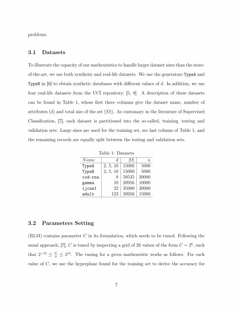
3.1 Datasets

To illustrate the capacity of our matheuristics to handle larger dataset sizes than the state-

of-the-art, we use both synthetic and real-life datasets. We use the generators TypeA and

TypeB in [6] to obtain synthetic databases with different values of d. In addition, we use

four real-life datasets from the UCI repository, [5, 8]. A description of these datasets

can be found in Table 1, whose first three columns give the dataset name, number of

attributes (d) and total size of the set (|Ω|). As customary in the literature of Supervised

Classification, [7], each dataset is partitioned into the so-called, training, testing and

validation sets. Large sizes are used for the training set, see last column of Table 1, and

the remaining records are equally split between the testing and validation sets.

Table 1: DatasetsName d |Ω| nTypeA 2, 5, 10 15000 5000TypeB 2, 5, 10 15000 5000cod-rna 8 59535 20000gamma 10 20956 10000ijcnn1 22 35000 20000adult 123 30956 15000

3.2 Parameters Setting

(RLM) contains parameter C in its formulation, which needs to be tuned. Following the

usual approach, [7], C is tuned by inspecting a grid of 26 values of the form C = 2k, such

that 2−12 ≤ Cn≤ 212. The tuning for a given matheuristic works as follows. For each

value of C, we use the hyperplane found for the training set to derive the accuracy for

7

the testing set. We choose the value of C maximizing the accuracy in the testing set, and

its accuracy on the validation test is reported.

In order to make a fair comparison, overall time limits for both Matheuristics 2 and

3 should be the same. Matheuristic 1 involves solving one (LSP) plus 26 (RLM), which

are aborted when a time limit is exceeded. In our experiments we choose tlimLSP =

300 seconds for (LSP), and for each (RLM) tlim1 is chosen as the closest integer tod+ n

100

5.

Matheuristic 3 involves solving 26 (RLM), which are aborted after tlim3 = tlim1+ tlimLSP

26.

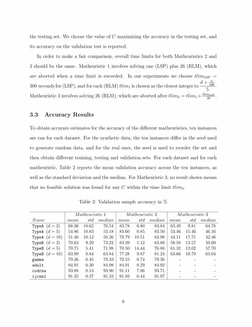
3.3 Accuracy Results

To obtain accurate estimates for the accuracy of the different matheuristics, ten instances

are run for each dataset. For the synthetic data, the ten instances differ in the seed used

to generate random data, and for the real ones, the seed is used to reorder the set and

then obtain different training, testing and validation sets. For each dataset and for each

matheuristic, Table 2 reports the mean validation accuracy across the ten instances, as

well as the standard deviation and the median. For Matheuristic 3, no result shown means

that no feasible solution was found for any C within the time limit tlim3.

Table 2: Validation sample accuracy in %

Matheuristic 1 Matheuristic 2 Matheuristic 3Name mean std median mean std median mean std median

TypeA (d = 2) 68.36 18.62 76.54 83.78 0.80 83.84 63.49 9.81 64.78TypeA (d = 5) 54.86 10.83 53.18 83.60 0.85 83.50 53.46 15.46 46.16TypeA (d = 10) 51.46 10.12 50.26 79.79 10.51 82.98 44.11 17.71 42.46TypeB (d = 2) 70.63 9.29 73.22 83.39 1.12 83.80 58.58 13.57 50.00TypeB (d = 5) 70.71 5.41 71.98 70.50 14.44 76.88 61.32 12.02 57.70TypeB (d = 10) 63.99 8.84 63.84 77.28 9.87 81.24 63.66 10.79 63.04gamma 79.26 0.45 79.33 79.55 0.74 79.36 - - -adult 84.91 0.30 84.98 84.91 0.29 84.92 - - -codrna 93.88 0.13 93.90 91.11 7.86 93.71 - - -ijcnn1 91.35 0.37 91.33 91.93 0.44 91.97 - - -

8

From Table 2, we can draw the following conclusions. Matheuristic 3 is not able to find

any feasible solution for the real-life datasets tested. Matheuristics 1 and 2 have a similar

accuracy, in terms of mean and median, in the real-life datasets. In TypeA, Matheuristic 2

clearly outperforms Matheuristics 1 and 3, while Matheuristic 1 outperforms Matheuris-

tic 3 in terms of median accuracy. In TypeB, Matheuristic 2 outperforms Matheuristic 3.

Matheuristic 1 outperforms Matheuristic 3 for d = 2, 10, while for d = 5 they are compa-

rable. Matheuristic 2 outperforms Matheuristic 1 in terms of median accuracy, where in

terms of mean accuracy the same holds for d = 2, 10, while for d = 5 the mean accuracies

are comparable.

Recall that for each dataset we are running 10 instances. In the following we focus

on the first of those instances, but the rest show a similar pattern. In Figures 1-10, we

plot the training accuracy as a function of C for the ten datasets tested. In Figures 1–

6, the ones corresponding to the synthetic datasets, one can see that the dominance of

Matheuristics 1 and 2 over 3 is very strong, since for every value of C Matheuristic 3 is

outperformed by our Matheuristics 1 and 2. Figures 7–10 reiterate that, for the real-life

datasets, Matheuristic 3 cannot find a solution for any value of C, while this is less of an

issue for Matheuristic 2. To conclude, as we are dealing with 10 different datasets and 10

instances for each of them, with 26 values of C, we are solving 2600 problems for which in

2393 of them Matheuristic 2 outperforms Matheuristic 3, that is, Matheuristic 2 succeeds

in 92.04% of the cases, while Matheuristic 1 outperforms Matheuristic 3 in the 76.58% of

the cases.

4 Conclusions

In this note we show that a quick heuristic, based on solving the continuous relaxation

of (RLM), is competitive against the state-of-the-art for ψ-learning, (RLM). Much better

9

results are obtained with our so-called Matheuristic 2, which involves solving an ILP and

a convex quadratic problem to obtain a good starting solution for the branch and bound.

In order to solve problems of larger size, valid cuts strengthening the formulation

would be extremely helpful. In this sense, [6] proposes the so-called geometric cuts,

but also mentions that these cuts are not suitable for d > 2, thus ignoring them in the

computational results. New and helpful cuts deserve further study.

References

[1] IBM ILOG CPLEX. www-01.ibm.com/software/integration/optimization/cplex-

optimizer, 2012.

[2] C. Apte. The big (data) dig. OR/MS Today, page 24, February 2003.

[3] B. Baesens, R. Setiono, C. Mues, and J. Vanthienen. Using neural network rule

extraction and decision tables for credit-risk evaluation. Management Science,

49(3):312–329, 2003.

[4] D. Bertsimas, M.V. Bjarnadóttir, M.A. Kane, J.Ch. Kryder, R. Pandey, S. Vempala,

and G. Wang. Algorithmic prediction of health-care costs. Operations Research,

56(6):1382–1392, 2008.

[5] C.L. Blake and C.J. Merz. UCI Repository of Machine Learning Databases.

http://www.ics.uci.edu/∼mlearn/MLRepository.html, 1998. University of Califor-

nia, Irvine, Department of Information and Computer Sciences.

[6] J. P. Brooks. Support vector machines with the ramp loss and the hard margin loss.

Operations Research, 59(2):467–479, 2011.

10

[7] E. Carrizosa and D. Romero Morales. Supervised classification and mathematical

optimization. Technical report, 2012. Forthcoming in Computers and Operations

Research.

[8] C. C. Chang and C. J. Lin. LIBSVM: a library for support vector machines. ACM

Transactions on Intelligent Systems and Technology, 2:1–27, 2011.

[9] W. A. Chaovalitwongse, Y.-J. Fan, and R. C. Sachdeo. Novel optimization models for

abnormal brain activity classification. Operations Research, 56(6):1450–1460, 2008.

[10] R. Collobert, F. Sinz, J. Weston, and L. Bottou. Trading convexity for scalability.

In Proceedings of the 23rd International Conference on Machine Learning, ICML06,

pages 201–208, New York, USA, 2006.

[11] N. Cristianini and J. Shawe-Taylor. An Introduction to Support Vector Machines and

Other Kernel-based Learning Methods. Cambridge University Press, 2000.

[12] I. Guyon, J. Weston, S. Barnhill, and V. Vapnik. Gene selection for cancer classifi-

cation using support vector machines. Machine Learning, 46:389–422, 2002.

[13] J. Han, R.B. Altman, V. Kumar, H. Mannila, and D. Pregibon. Emerging scientific

applications in data mining. Communications of the ACM, 45(8):54–58, 2002.

[14] H. Hand, H. Mannila, and P. Smyth. Principles of Data Mining. MIT Press, 2001.

[15] T. Hastie, R. Tibshirani, and J. Friedman. The Elements of Statistical Learning.

Springer, New York, 2001.

[16] Y. Liu and Y. Wu. Optimizing ψ-learning via mixed integer programming. Statistica

Sinica, 16:441–457, 2006.

[17] G. Loveman. Diamonds in the data mine. Harvard Business Review, 81(5):109–113,

2003.

11

[18] O.L. Mangasarian, W.N. Street, and W.H. Wolberg. Breast cancer diagnosis and

prognosis via linear programming. Operations Research, 43(4):570–577, 1995.

[19] X. Shen, G. C. Tseng, X. Zhang, and W. H. Wong. On ψ-learning. Journal of the

American Statistical Association, 98:724–734, 2003.

[20] V. Vapnik. The Nature of Statistical Learning Theory. Springer-Verlag, 1995.

[21] V. Vapnik. Statistical Learning Theory. Wiley, 1998.

[22] X. Wu, V. Kumar, J. Ross Quinlan, J. Ghosh, Q. Yang, H. Motoda, G. J. McLachlan,

A. Ng, B. Liu, P. S. Yu, Z.-H. Zhou, M. Steinbach, D. J. Hand, and D. Steinberg.

Top 10 algorithms in data mining. Knowledge and Information Systems, 14:1–37,

2007.

12

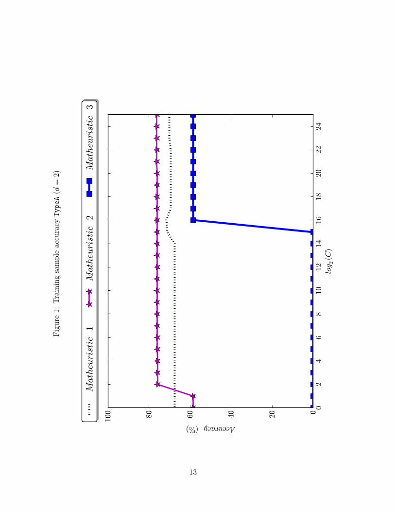
Figure1:

Training

sampleaccuracy

TypeA

(d=

2)

02

46

810

1214

1618

2022

24log 2

(C)

020406080100

Accuracy(%)Matheuristic

1Matheuristic

2Matheuristic

3

13

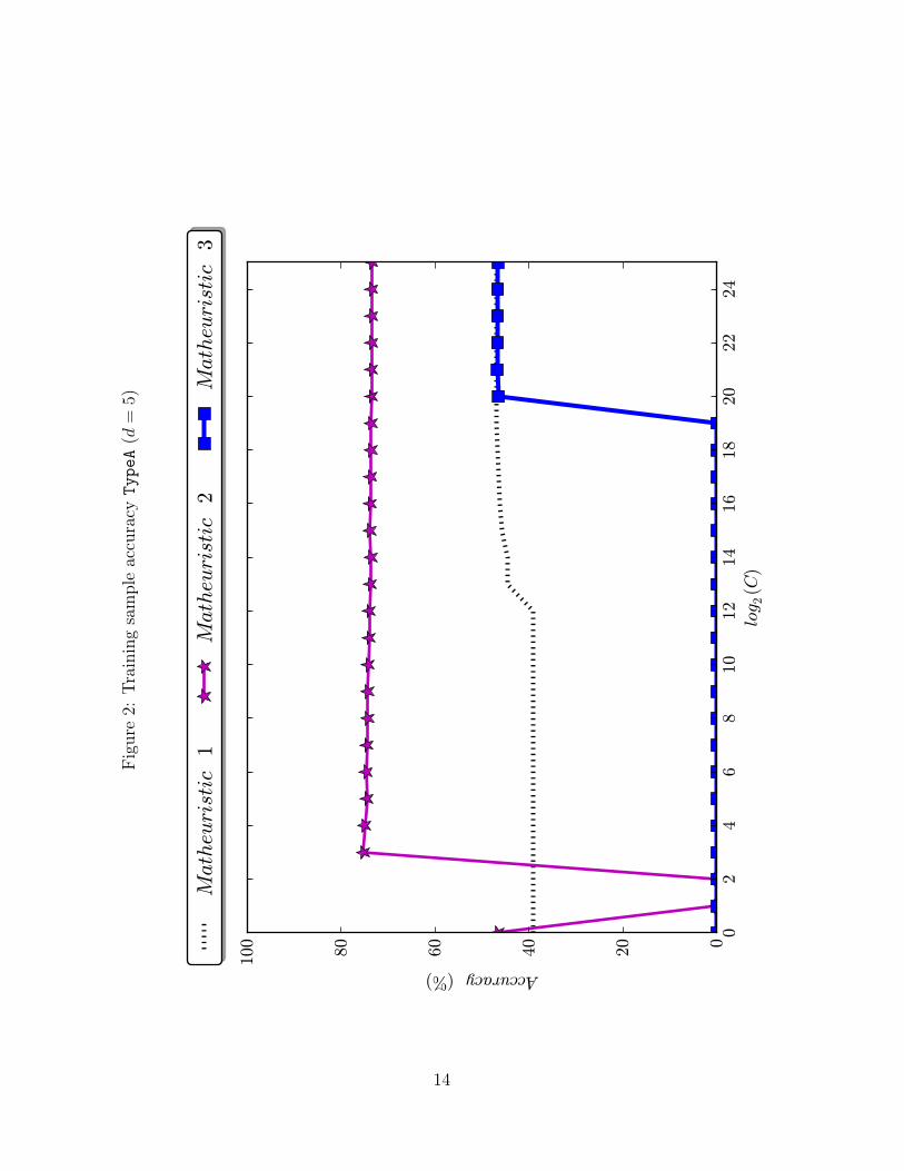
Figure2:

Training

sampleaccuracy

TypeA

(d=

5)

02

46

810

1214

1618

2022

24log 2

(C)

020406080100

Accuracy(%)Matheuristic

1Matheuristic

2Matheuristic

3

14

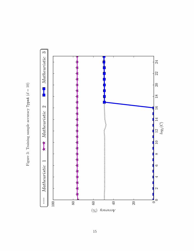
Figure3:

Training

sampleaccu

racy

TypeA

(d=

10)

02

46

810

1214

1618

2022

24log 2

(C)

020406080100

Accuracy(%)Matheuristic

1Matheuristic

2Matheuristic

3

15

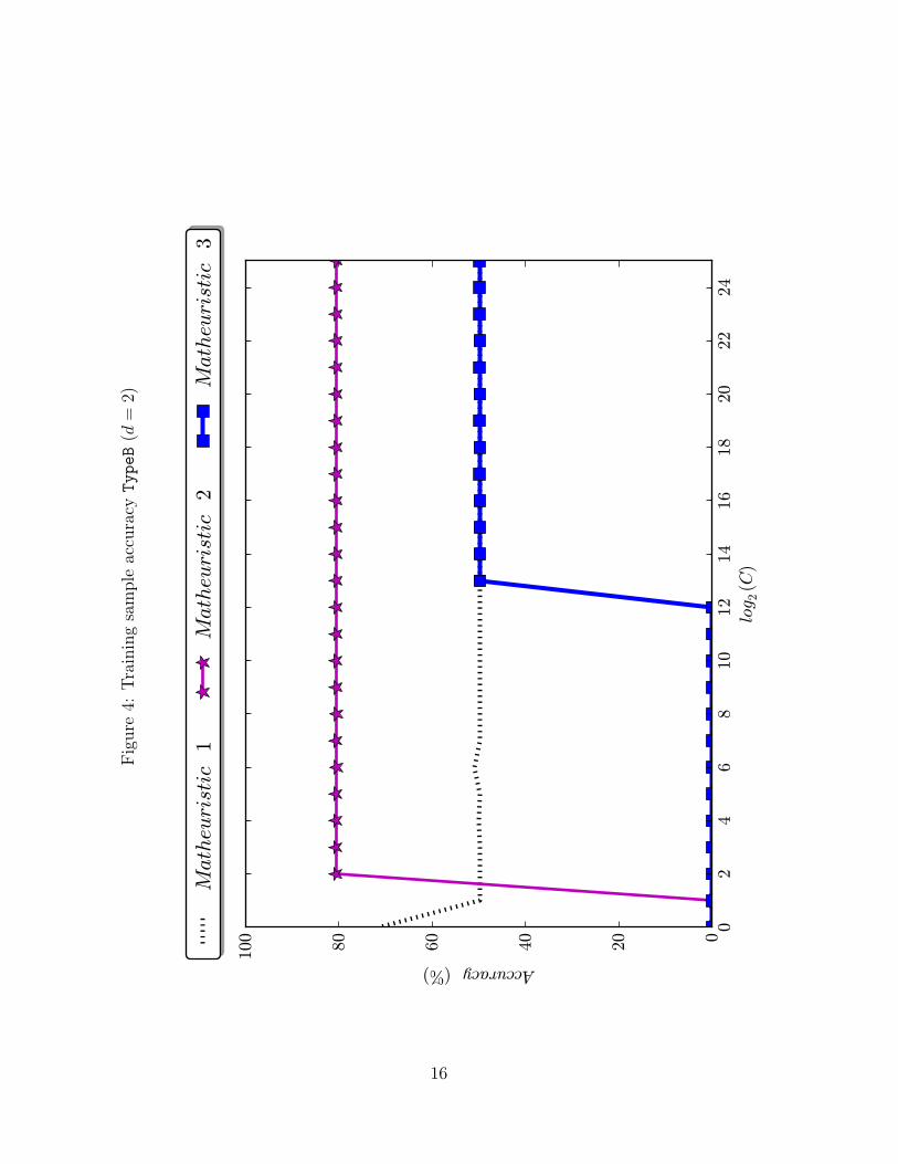
Figure4:

Training

sampleaccuracy

TypeB

(d=

2)

02

46

810

1214

1618

2022

24log 2

(C)

020406080100

Accuracy(%)Matheuristic

1Matheuristic

2Matheuristic

3

16

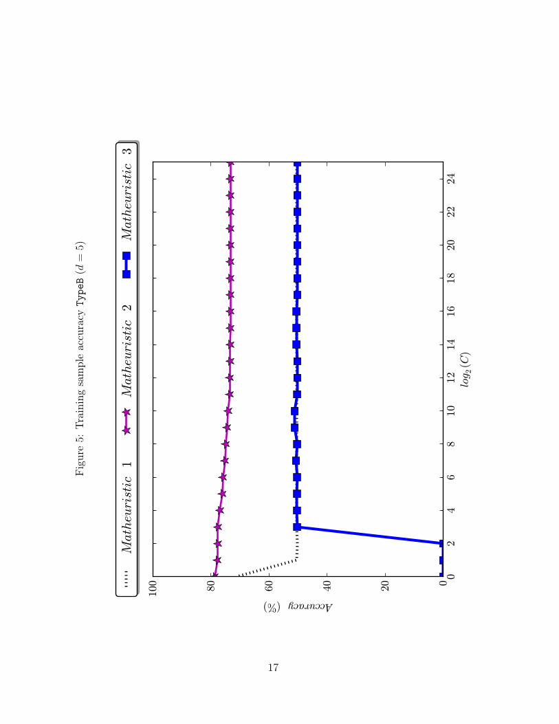
Figure5:

Training

sampleaccuracy

TypeB

(d=

5)

02

46

810

1214

1618

2022

24log 2

(C)

020406080100

Accuracy(%)Matheuristic

1Matheuristic

2Matheuristic

3

17

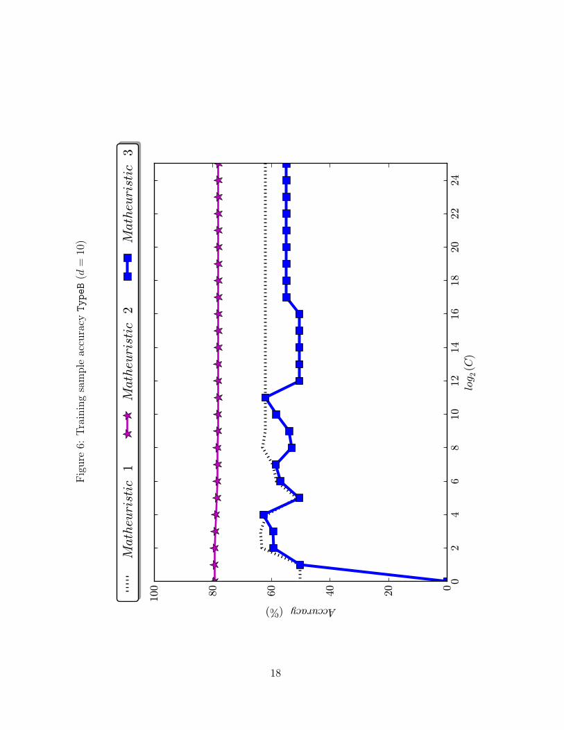
Figure6:

Training

sampleaccu

racy

TypeB

(d=

10)

02

46

810

1214

1618

2022

24log 2

(C)

020406080100

Accuracy(%)Matheuristic

1Matheuristic

2Matheuristic

3

18

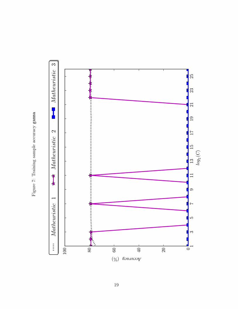
Figure7:

Training

sampleaccu

racy

gamm

a

13

57

911

1315

1719

2123

25

log 2

(C)

020406080100

Accuracy(%)Matheuristic

1Matheuristic

2Matheuristic

3

19

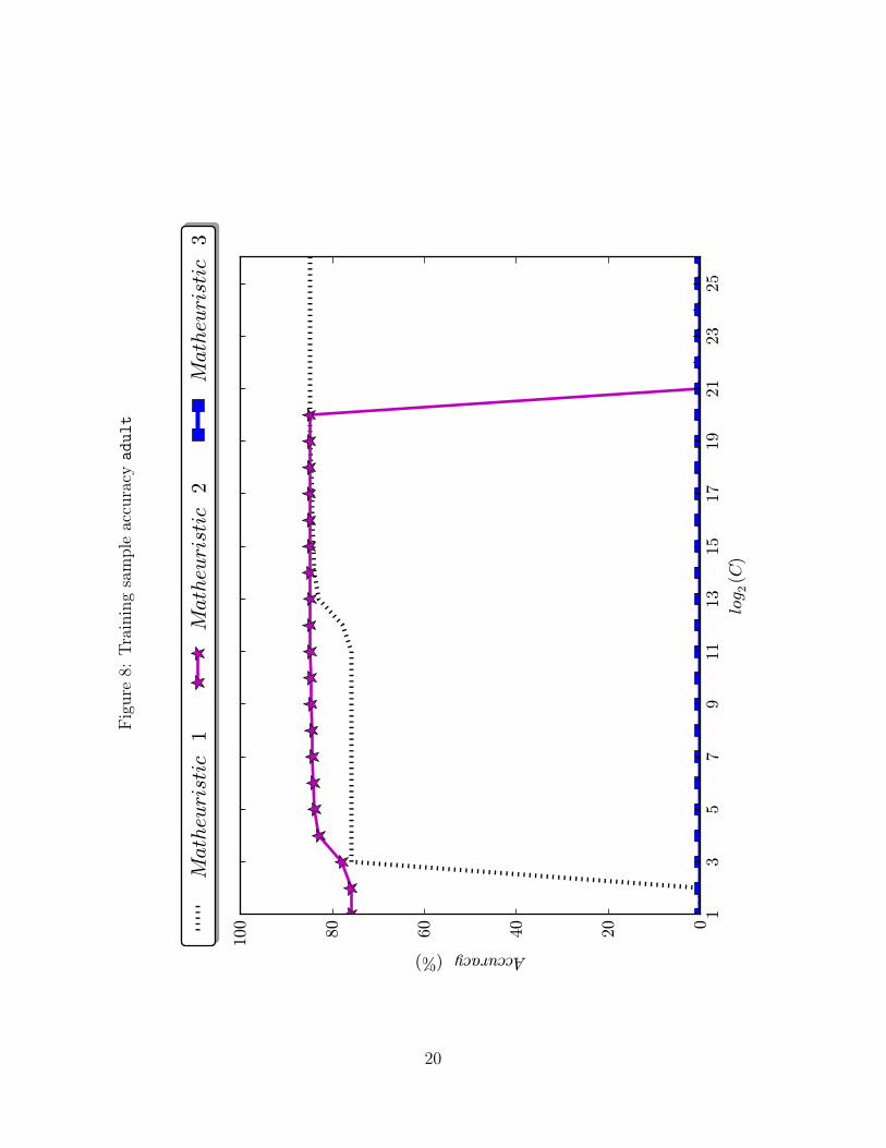
Figure8:

Training

sampleaccu

racy

adul

t

13

57

911

1315

1719

2123

25

log 2

(C)

020406080100

Accuracy(%)Matheuristic

1Matheuristic

2Matheuristic

3

20

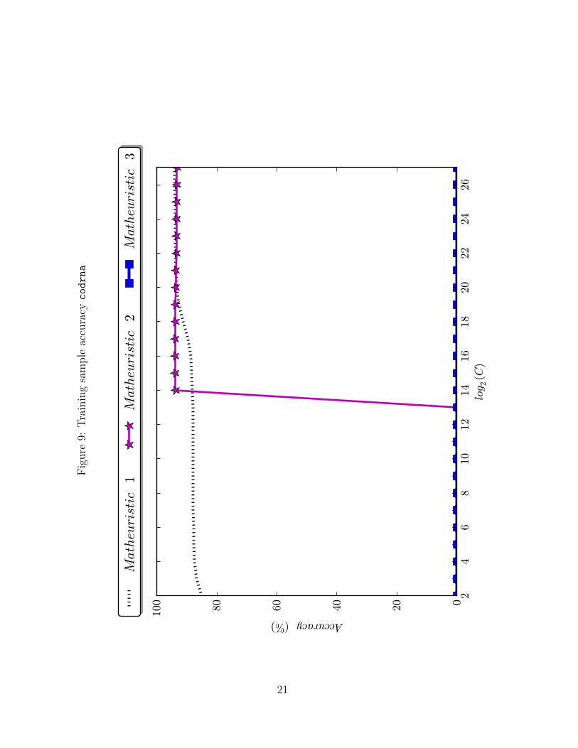
Figure9:

Training

sampleaccu

racy

codr

na

24

68

1012

1416

1820

2224

26log 2

(C)

020406080100

Accuracy(%)Matheuristic

1Matheuristic

2Matheuristic

3

21

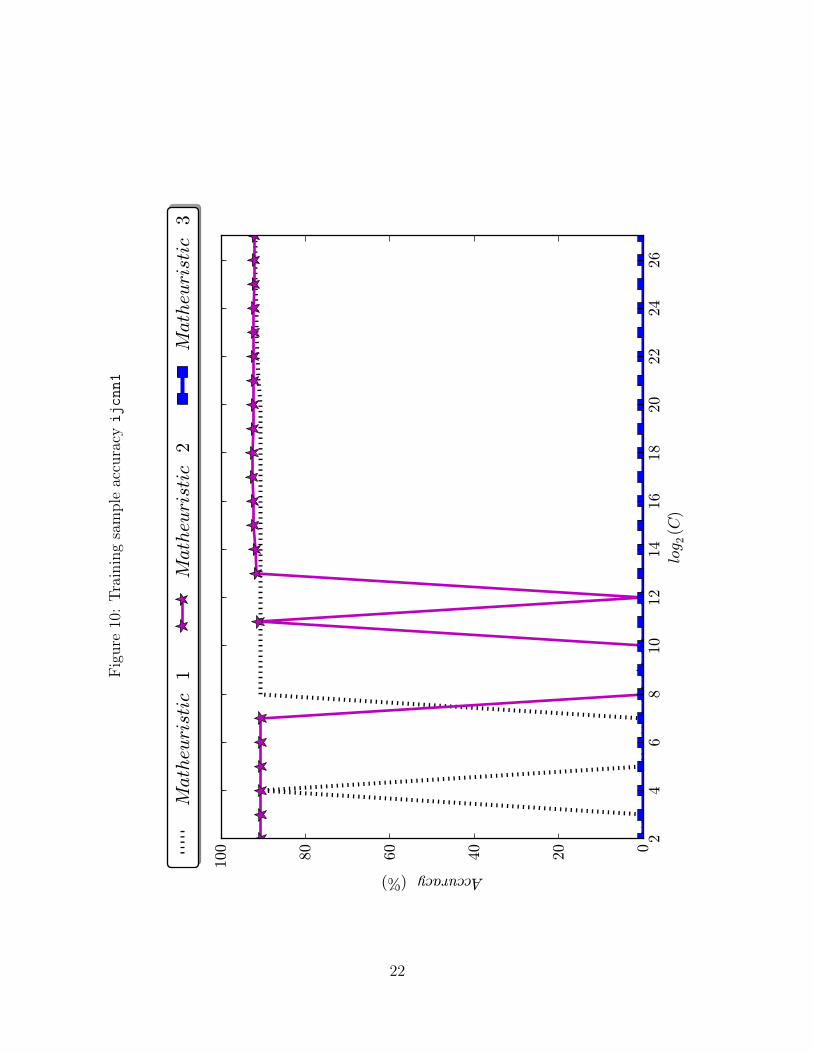
Figure10

:Tr

aining

sampleaccuracy

ijcn

n1

24

68

1012

1416

1820

2224

26log 2

(C)

020406080100

Accuracy(%)Matheuristic

1Matheuristic

2Matheuristic

3

22