Q-Function Learning Methods
21
Q-Function Learning Methods February 15, 2017
Transcript of Q-Function Learning Methods
Q-Function Learning Methods
February 15, 2017
Value Functions
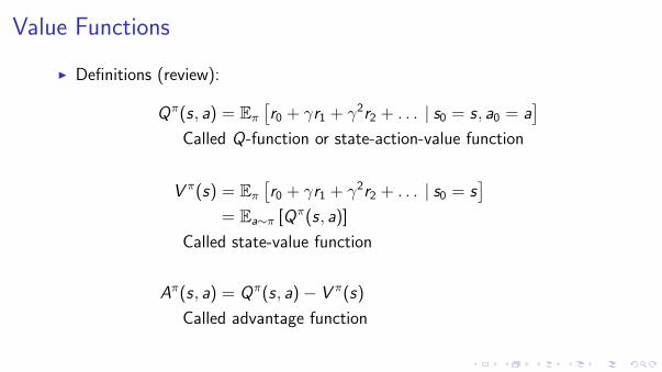
I Definitions (review):
Qπ(s, a) = Eπ[r0 + γr1 + γ2r2 + . . . | s0 = s, a0 = a
]Called Q-function or state-action-value function
V π(s) = Eπ[r0 + γr1 + γ2r2 + . . . | s0 = s
]= Ea∼π [Qπ(s, a)]
Called state-value function
Aπ(s, a) = Qπ(s, a)− V π(s)
Called advantage function
Bellman Equations for Qπ
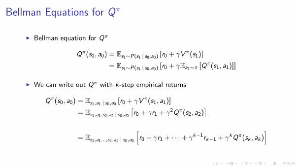
I Bellman equation for Qπ
Qπ(s0, a0) = Es1∼P(s1 | s0,a0) [r0 + γV π(s1)]
= Es1∼P(s1 | s0,a0) [r0 + γEa1∼π [Qπ(s1, a1)]]
I We can write out Qπ with k-step empirical returns
Qπ(s0, a0) = Es1,a1 | s0,a0[r0 + γV π(s1, a1)]
= Es1,a1,s2,a2 | s0,a0
[r0 + γr1 + γ2Qπ(s2, a2)
]= Es1,a1...,sk ,ak | s0,a0
[r0 + γr1 + · · ·+ γk−1rk−1 + γkQπ(sk , ak)
]
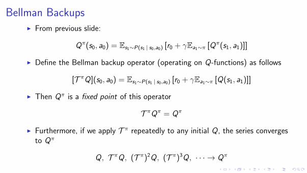
Bellman BackupsI From previous slide:
Qπ(s0, a0) = Es1∼P(s1 | s0,a0) [r0 + γEa1∼π [Qπ(s1, a1)]]
I Define the Bellman backup operator (operating on Q-functions) as follows
[T πQ](s0, a0) = Es1∼P(s1 | s0,a0) [r0 + γEa1∼π [Q(s1, a1)]]
I Then Qπ is a fixed point of this operator
T πQπ = Qπ
I Furthermore, if we apply T π repeatedly to any initial Q, the series convergesto Qπ
Q, T πQ, (T π)2Q, (T π)3Q, · · · → Qπ
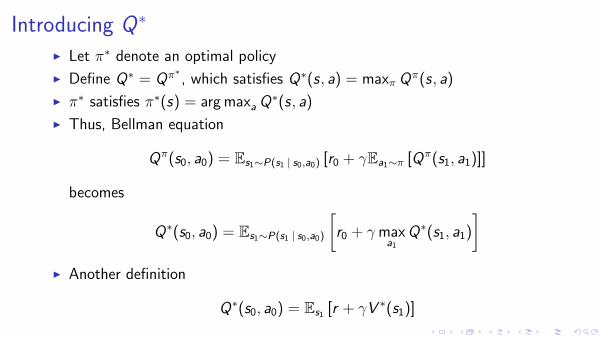
Introducing Q∗
I Let π∗ denote an optimal policy
I Define Q∗ = Qπ∗, which satisfies Q∗(s, a) = maxπ Q
π(s, a)
I π∗ satisfies π∗(s) = arg maxa Q∗(s, a)
I Thus, Bellman equation
Qπ(s0, a0) = Es1∼P(s1 | s0,a0) [r0 + γEa1∼π [Qπ(s1, a1)]]
becomes
Q∗(s0, a0) = Es1∼P(s1 | s0,a0)
[r0 + γ max
a1
Q∗(s1, a1)
]I Another definition
Q∗(s0, a0) = Es1 [r + γV ∗(s1)]
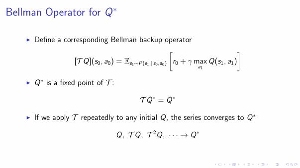
Bellman Operator for Q∗
I Define a corresponding Bellman backup operator
[T Q](s0, a0) = Es1∼P(s1 | s0,a0)
[r0 + γ max
a1
Q(s1, a1)
]I Q∗ is a fixed point of T :
T Q∗ = Q∗
I If we apply T repeatedly to any initial Q, the series converges to Q∗
Q, T Q, T 2Q, · · · → Q∗
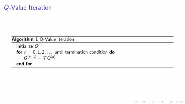
Q-Value Iteration
Algorithm 1 Q-Value Iteration
Initialize Q(0)
for n = 0, 1, 2, . . . until termination condition doQ(n+1) = T Q(n)
end for
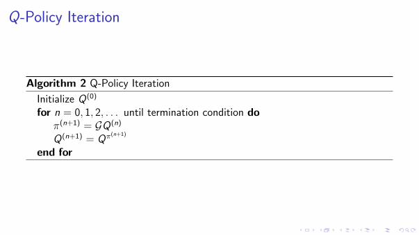
Q-Policy Iteration
Algorithm 2 Q-Policy Iteration
Initialize Q(0)
for n = 0, 1, 2, . . . until termination condition doπ(n+1) = GQ(n)
Q(n+1) = Qπ(n+1)
end for
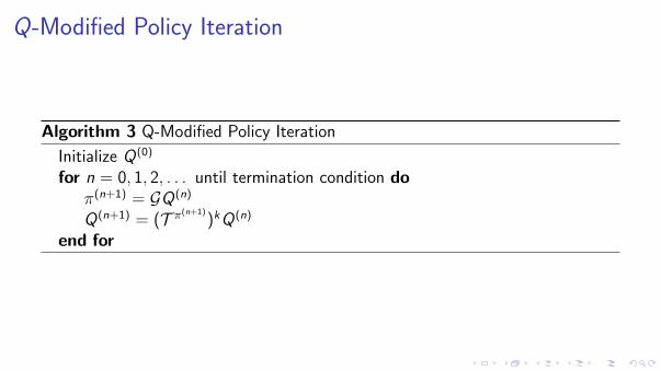
Q-Modified Policy Iteration
Algorithm 3 Q-Modified Policy Iteration
Initialize Q(0)
for n = 0, 1, 2, . . . until termination condition doπ(n+1) = GQ(n)
Q(n+1) = (T π(n+1))kQ(n)
end for
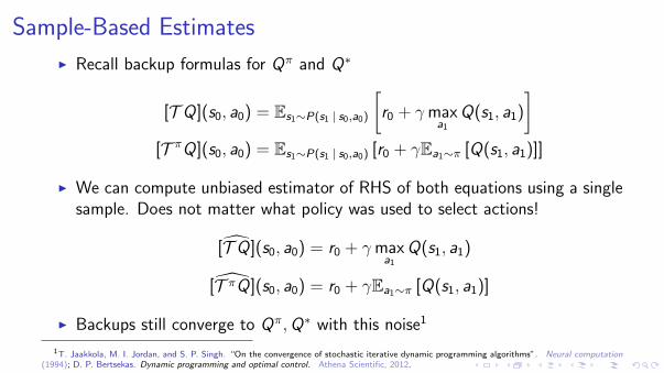
Sample-Based Estimates
I Recall backup formulas for Qπ and Q∗
[T Q](s0, a0) = Es1∼P(s1 | s0,a0)
[r0 + γ max
a1
Q(s1, a1)
][T πQ](s0, a0) = Es1∼P(s1 | s0,a0) [r0 + γEa1∼π [Q(s1, a1)]]
I We can compute unbiased estimator of RHS of both equations using a singlesample. Does not matter what policy was used to select actions!
[T̂ Q](s0, a0) = r0 + γ maxa1
Q(s1, a1)
[T̂ πQ](s0, a0) = r0 + γEa1∼π [Q(s1, a1)]
I Backups still converge to Qπ,Q∗ with this noise1
1T. Jaakkola, M. I. Jordan, and S. P. Singh. “On the convergence of stochastic iterative dynamic programming algorithms”. Neural computation(1994); D. P. Bertsekas. Dynamic programming and optimal control. Athena Scientific, 2012.
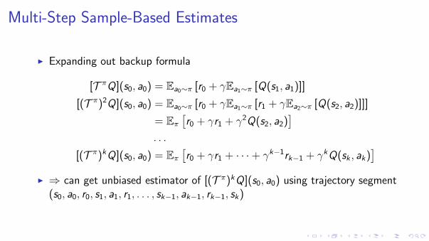
Multi-Step Sample-Based Estimates
I Expanding out backup formula
[T πQ](s0, a0) = Ea0∼π [r0 + γEa1∼π [Q(s1, a1)]]
[(T π)2Q](s0, a0) = Ea0∼π [r0 + γEa1∼π [r1 + γEa2∼π [Q(s2, a2)]]]
= Eπ[r0 + γr1 + γ2Q(s2, a2)
]. . .
[(T π)kQ](s0, a0) = Eπ[r0 + γr1 + · · ·+ γk−1rk−1 + γkQ(sk , ak)
]I ⇒ can get unbiased estimator of [(T π)kQ](s0, a0) using trajectory segment
(s0, a0, r0, s1, a1, r1, . . . , sk−1, ak−1, rk−1, sk)
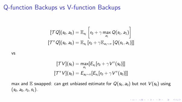
Q-function Backups vs V-function Backups
[T Q](s0, a0) = Es1
[r0 + γ max
a1
Q(s1, a1)
][T πQ](s0, a0) = Es1 [r0 + γEa1∼π [Q(s1, a1)]]
vs
[T V ](s0) = maxa1
[Es1[r0 + γV π(s0)]]
[T πV ](s0) = Ea0∼π[Es1[r0 + γV π(s0)]]
max and E swapped: can get unbiased estimate for Q(s0, a0) but not V (s0) using(s0, a0, r0, s1).
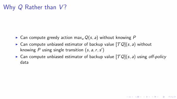
Why Q Rather than V ?
I Can compute greedy action maxa Q(s, a) without knowing P
I Can compute unbiased estimator of backup value [T Q](s, a) withoutknowing P using single transition (s, a, r , s ′)
I Can compute unbiased estimator of backup value [T Q](s, a) using off-policydata
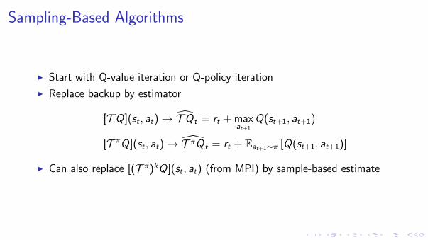
Sampling-Based Algorithms
I Start with Q-value iteration or Q-policy iteration
I Replace backup by estimator
[T Q](st , at)→ T̂ Qt = rt + maxat+1
Q(st+1, at+1)
[T πQ](st , at)→ T̂ πQt = rt + Eat+1∼π [Q(st+1, at+1)]
I Can also replace [(T π)kQ](st , at) (from MPI) by sample-based estimate
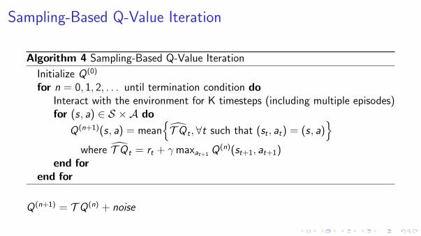
Sampling-Based Q-Value Iteration
Algorithm 4 Sampling-Based Q-Value Iteration
Initialize Q(0)
for n = 0, 1, 2, . . . until termination condition doInteract with the environment for K timesteps (including multiple episodes)for (s, a) ∈ S ×A do
Q(n+1)(s, a) = mean{T̂ Qt ,∀t such that (st , at) = (s, a)
}where T̂ Qt = rt + γ maxat+1 Q
(n)(st+1, at+1)end for
end for
Q(n+1) = T Q(n) + noise
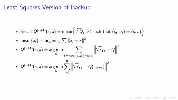
Least Squares Version of Backup
I Recall Q(n+1)(s, a) = mean{T̂ Qt ,∀t such that (st , at) = (s, a)
}I mean{x̂i} = arg minx
∑i‖xi − x‖2
I Q(n+1)(s, a) = arg minQ
∑t where (st ,at)=(s,a)
∥∥∥T̂ Qt − Q∥∥∥2
I Q(n+1)(s, a) = arg minQ
K∑t=1
∥∥∥T̂ Qt − Q(st , at)∥∥∥2
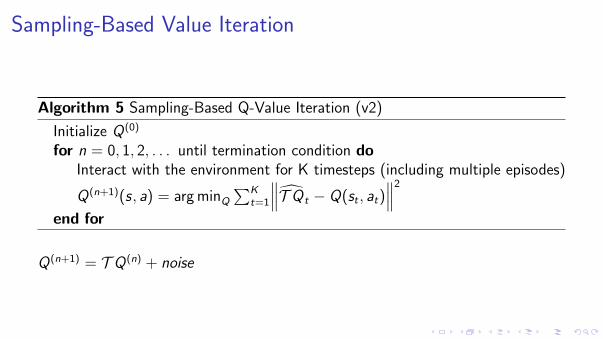
Sampling-Based Value Iteration
Algorithm 5 Sampling-Based Q-Value Iteration (v2)
Initialize Q(0)
for n = 0, 1, 2, . . . until termination condition doInteract with the environment for K timesteps (including multiple episodes)
Q(n+1)(s, a) = arg minQ
∑Kt=1
∥∥∥T̂ Qt − Q(st , at)∥∥∥2
end for
Q(n+1) = T Q(n) + noise
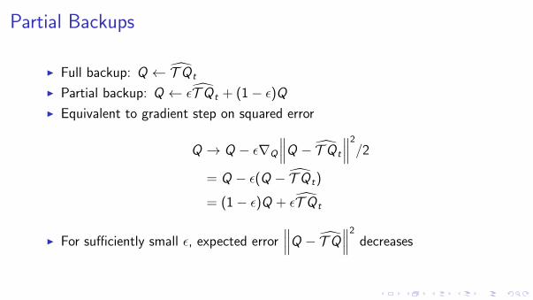
Partial Backups
I Full backup: Q ← T̂ Qt
I Partial backup: Q ← εT̂ Qt + (1− ε)QI Equivalent to gradient step on squared error
Q → Q − ε∇Q
∥∥∥Q − T̂ Qt
∥∥∥2
/2
= Q − ε(Q − T̂ Qt)
= (1− ε)Q + εT̂ Qt
I For sufficiently small ε, expected error∥∥∥Q − T̂ Q∥∥∥2
decreases

Sampling-Based Q-Value Iteration
Algorithm 6 Sampling-Based Q-Value Iteration (v3)
Initialize Q(0)
for n = 0, 1, 2, . . . until termination condition doInteract with the environment for K timesteps (including multiple episodes)
Q(n+1) = Q(n) + ε∇Q
∑Kt=1
∥∥∥T̂ Qt − Q(st , at)∥∥∥2
/2
end for
Q(n+1) = Q(n) + ε
(∇Q
∥∥∥T Q(n) − Q∥∥∥2
/2∣∣Q=Q(n) + noise
)= argmin
Q
∥∥∥(1− ε)Q(n) + ε(T Q(n) + noise)∥∥∥2
I K = 1⇒ Watkins’ Q-learning2
I Large K : batch Q-value iteration2C. J. Watkins and P. Dayan. “Q-learning”. Machine learning (1992).
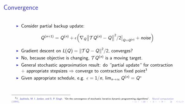
Convergence
I Consider partial backup update:
Q(n+1) = Q(n) + ε(∇Q
∥∥T Q(n) − Q∥∥2/2∣∣Q=Q(n) + noise
)I Gradient descent on L(Q) = ‖T Q − Q‖2/2, converges?
I No, because objective is changing, T Q(n) is a moving target.
I General stochastic approximation result: do “partial update“ for contraction+ appropriate stepsizes ⇒ converge to contraction fixed point3
I Given appropriate schedule, e.g. ε = 1/n, limn→∞Q(n) = Q∗
3T. Jaakkola, M. I. Jordan, and S. P. Singh. “On the convergence of stochastic iterative dynamic programming algorithms”. Neural computation(1994).

Function Approximation / Neural-Fitted AlgorithmsI Parameterize Q-function with a neural network Qθ
I To approximate Q ← T̂ Q, do
minimizeθ
∑t
∥∥∥Qθ(st , at)− T̂ Q(st , at)∥∥∥2
Algorithm 7 Neural-Fitted Q-Iteration (NFQ)4
I Initialize θ(0).for n = 1, 2, . . . do
Sample trajectory using policy π(n).
θ(n) = minimizeθ∑
t
(T̂ Qt − Qθ(st , at)
)2
end for
4M. Riedmiller. “Neural fitted Q iteration–first experiences with a data efficient neural reinforcement learning method”. Machine Learning:ECML 2005. Springer, 2005.