Advanced Machine Learning & Perception
21
Tony Jebara, Columbia University Advanced Machine Learning & Perception Instructor: Tony Jebara
Transcript of Advanced Machine Learning & Perception
Tony Jebara, Columbia University
Advanced Machine Learning & Perception
Instructor: Tony Jebara
Tony Jebara, Columbia University
Multi-Task Learning • Review MED SVM
• MED Feature Selection
• MED Kernel Selection
• Multi-Task MED
• Adaptive Pooling

Tony Jebara, Columbia University
SVM Extensions Classification Regression
Feature/Kernel Selection Meta/Multi-Task Learning
Transduction Multi-Class / Structured
x x x x x x x x x x
x x
x x x x
x
x x x
x x x
x x x x
x
x
x x x x x
? ? ? ?
? O
? ? ?
? ? ?
? ? X ? ? ? ?
? ? ?
x x x x
x x
x x x
x x x
O O O
O O
O O O
O O
x x x
x x
x x O O O O
O O O
x x
x x O O
O O x O
x x x O O
x x x x
x x
x x x x
O O O O
O O O
O O
+ + + +
+ +
Tony Jebara, Columbia University
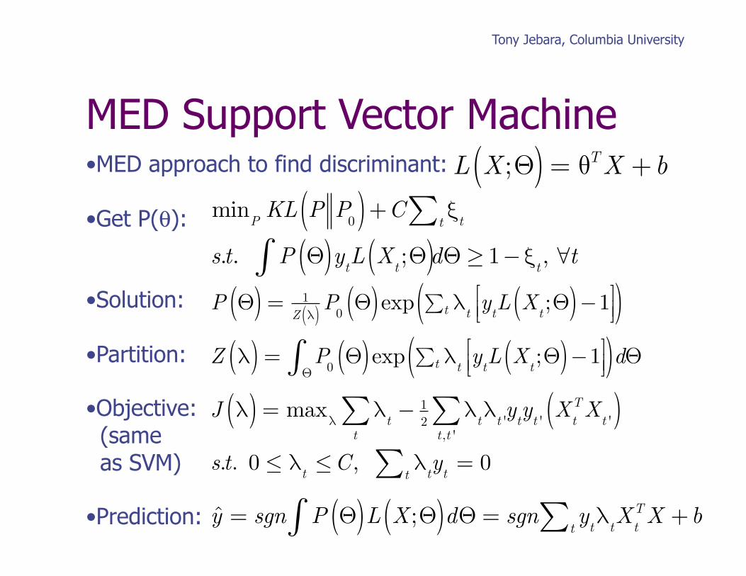
• MED approach to find discriminant:
• Get P(θ):
• Solution:
• Partition:
• Objective: (same as SVM)
• Prediction:
MED Support Vector Machine
y = sgn P Θ( )L X;Θ( )dΘ∫ = sgn y
tλ
tX
tTX
t∑ +b
minPKL P P
0( ) +C ξtt∑
s.t. P Θ( )ytL X
t;Θ( )∫ dΘ≥ 1−ξ
t, ∀t
P Θ( ) = 1
Z λ( ) P0Θ( )exp λ
ty
tL X
t;Θ( )−1⎡
⎣⎢⎤⎦⎥t∑( )
Z λ( ) = P
0Θ( )exp λ
ty
tL X
t;Θ( )−1⎡
⎣⎢⎤⎦⎥t∑( )d
Θ∫ Θ
J λ( ) = maxλλ
tt∑ − 1
2λ
tλ
t 'y
ty
t 'X
tTX
t '( )t,t '∑
s.t. 0 ≤ λt≤C, λ
ty
t= 0
t∑
L X;Θ( ) = θTX +b
Tony Jebara, Columbia University
MED Feature Selection
s
i∈ 0,1{ }
P
s,0s
i( ) = ρsi 1−ρ( )1−si P
0Θ,s( )
P Θ,s( )
x x x x x
x x x x x
L X;Θ( ) = s
iθ
iX
ii∑ +b
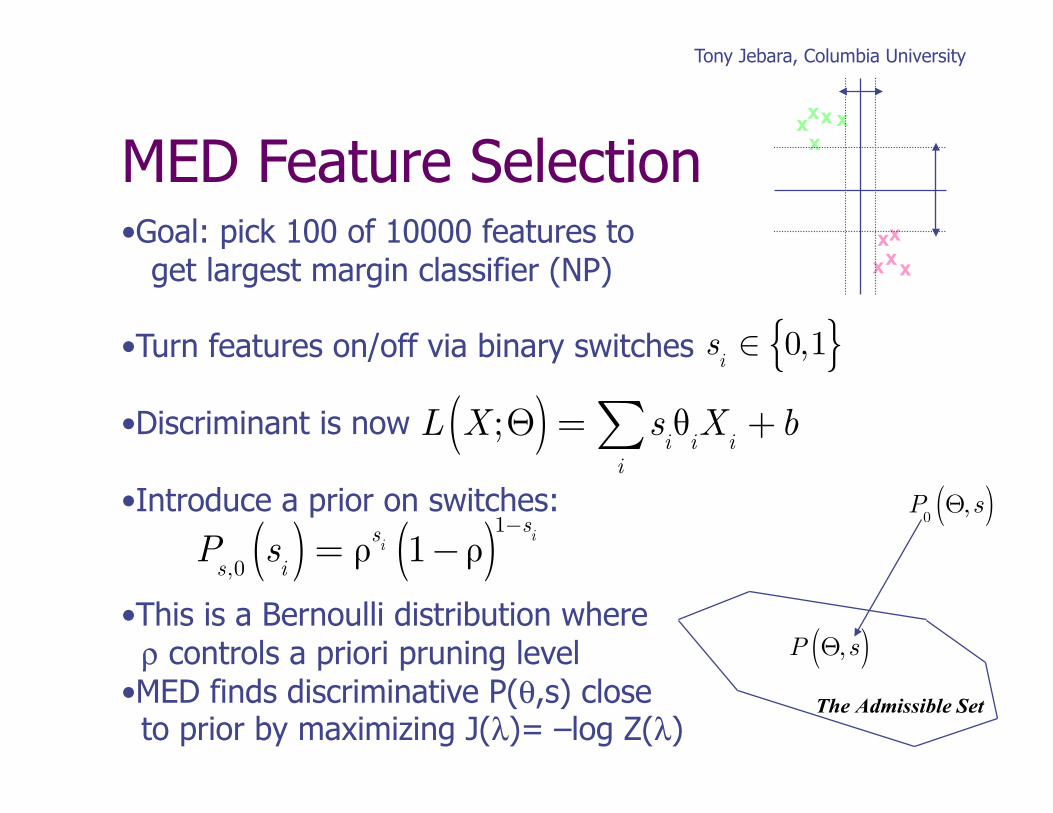
• Goal: pick 100 of 10000 features to get largest margin classifier (NP)
• Turn features on/off via binary switches
• Discriminant is now
• Introduce a prior on switches:
• This is a Bernoulli distribution where ρ controls a priori pruning level • MED finds discriminative P(θ,s) close to prior by maximizing J(λ)= –log Z(λ)
Tony Jebara, Columbia University
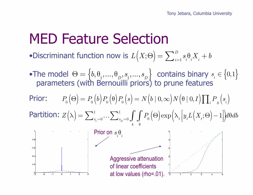
• Discriminant function now is
• The model contains binary parameters (with Bernouilli priors) to prune features
Prior:
Partition:
MED Feature Selection L X;Θ( ) = s
iθ
iX
ii=1
D∑ +b
Θ = b, θ
1,..., θ
D,s
1,...,s
D{ } s
i∈ 0,1{ }
P
0Θ( ) = P
0b( )P0
θ( )P0s( ) = N b | 0,∞( )N θ | 0,I( ) P
i∏ 0s
i( )
Aggressive attenuation of linear coefficients at low values (rho=.01).
Prior on siθ
i
Z λ( ) = … P
0Θ( )exp λ
ty
tL X
t;Θ( )−1⎡
⎣⎢⎤⎦⎥( )
θ
∫b
∫sD =0
1∑s1 =0
1∑ dθdb
Tony Jebara, Columbia University
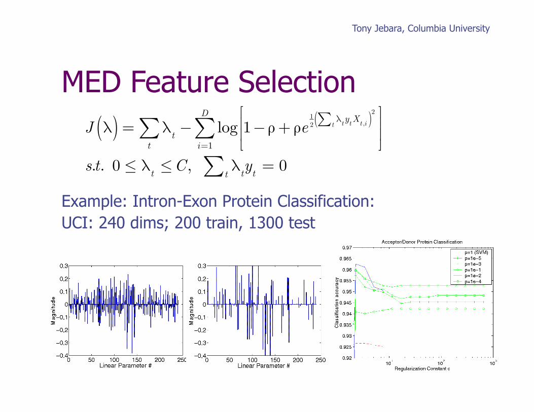
MED Feature Selection
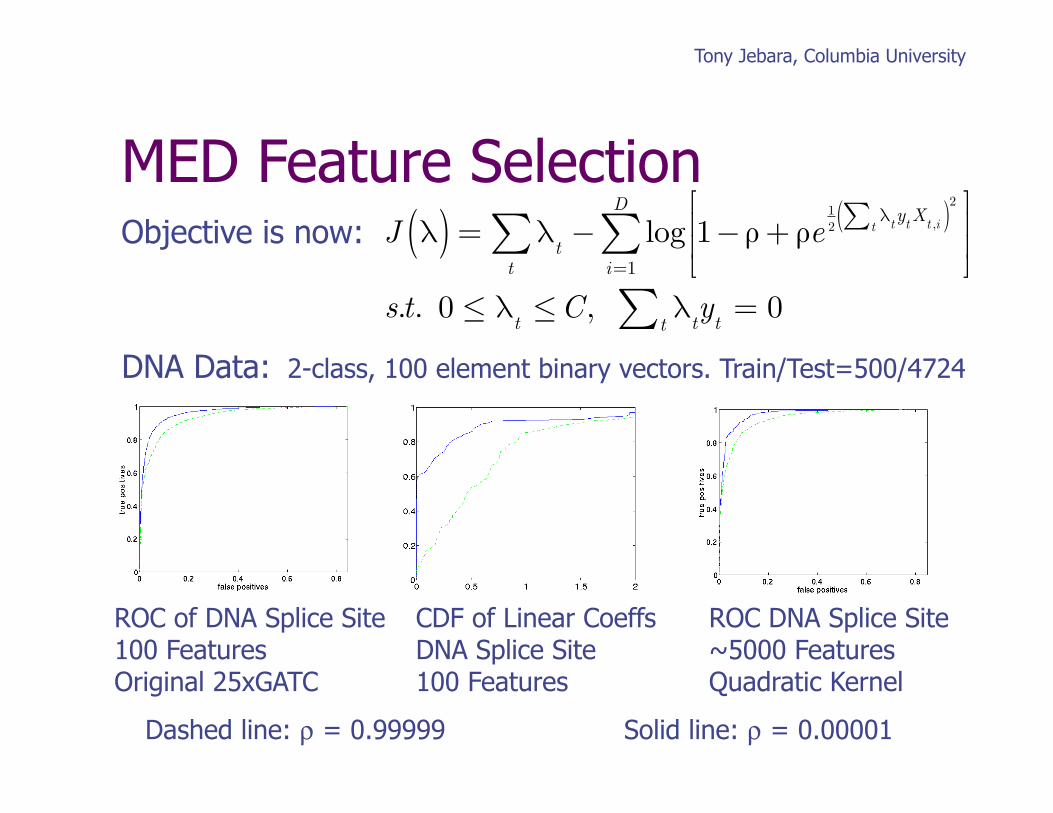
J λ( ) = λt
t∑ − log 1−ρ+ ρe
12
λtytXt ,it∑( )2⎡
⎣⎢⎢
⎤
⎦⎥⎥
i=1
D
∑s.t. 0 ≤ λ
t≤C, λ
ty
t= 0
t∑
ROC of DNA Splice Site 100 Features Original 25xGATC
ROC DNA Splice Site ~5000 Features Quadratic Kernel
CDF of Linear Coeffs DNA Splice Site 100 Features
Dashed line: ρ = 0.99999 Solid line: ρ = 0.00001
DNA Data: 2-class, 100 element binary vectors. Train/Test=500/4724
Objective is now:
Tony Jebara, Columbia University
MED Feature Selection
J λ( ) = λt
t∑ − log 1−ρ+ ρe
12
λtytXt ,it∑( )2⎡
⎣⎢⎢
⎤
⎦⎥⎥
i=1
D
∑s.t. 0 ≤ λ
t≤C, λ
ty
t= 0
t∑Example: Intron-Exon Protein Classification: UCI: 240 dims; 200 train, 1300 test
Tony Jebara, Columbia University
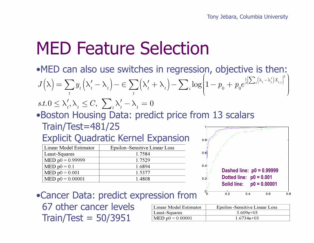
• MED can also use switches in regression, objective is then:
• Boston Housing Data: predict price from 13 scalars Train/Test=481/25 Explicit Quadratic Kernel Expansion
• Cancer Data: predict expression from 67 other cancer levels Train/Test = 50/3951
MED Feature Selection
J λ( ) = yt′λt−λ
t( )−t∑ ∈ ′λ
t+ λ
t( )t∑ − log 1− p
0+ p
0e
12
λt − ′λt( )Xt ,it∑⎡⎣⎢ ⎤⎦⎥2⎛
⎝⎜⎜⎜⎜
⎞
⎠⎟⎟⎟⎟i∑
s.t.0 ≤ ′λt,λ
t≤C, ′λ
t−λ
t= 0
t∑
Dashed line: p0 = 0.99999 Dotted line: p0 = 0.001 Solid line: p0 = 0.00001
Tony Jebara, Columbia University
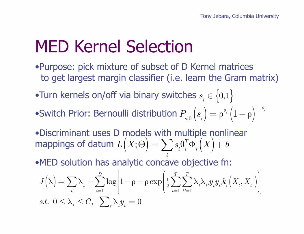
• Purpose: pick mixture of subset of D Kernel matrices to get largest margin classifier (i.e. learn the Gram matrix)
• Turn kernels on/off via binary switches
• Switch Prior: Bernoulli distribution
• Discriminant uses D models with multiple nonlinear mappings of datum
• MED solution has analytic concave objective fn:
MED Kernel Selection
s
i∈ 0,1{ }
P
s,0s
i( ) = ρsi 1−ρ( )1−si
L X;Θ( ) = s
iθ
iTΦ
iX( )
i∑ +b
J λ( ) = λt
t∑ − log 1−ρ+ ρ exp 1
2λ
tλ
t 'y
ty
t 'k
iX
t,X
t '( )t '=1
T
∑t=1
T
∑⎛
⎝⎜⎜⎜⎜
⎞
⎠⎟⎟⎟⎟
⎡
⎣
⎢⎢⎢
⎤
⎦
⎥⎥⎥i=1
D
∑
s.t. 0 ≤ λt≤C, λ
ty
t= 0
t∑
Tony Jebara, Columbia University
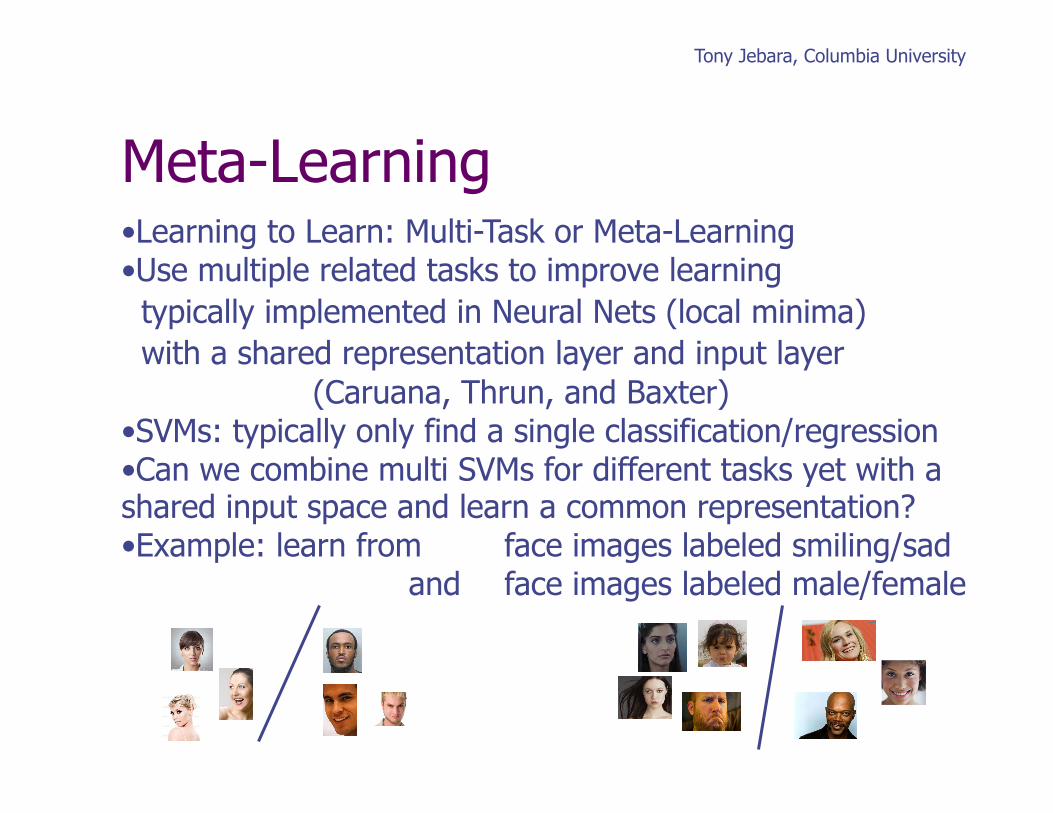
Meta-Learning • Learning to Learn: Multi-Task or Meta-Learning • Use multiple related tasks to improve learning typically implemented in Neural Nets (local minima) with a shared representation layer and input layer (Caruana, Thrun, and Baxter) • SVMs: typically only find a single classification/regression • Can we combine multi SVMs for different tasks yet with a shared input space and learn a common representation? • Example: learn from face images labeled smiling/sad and face images labeled male/female
Tony Jebara, Columbia University
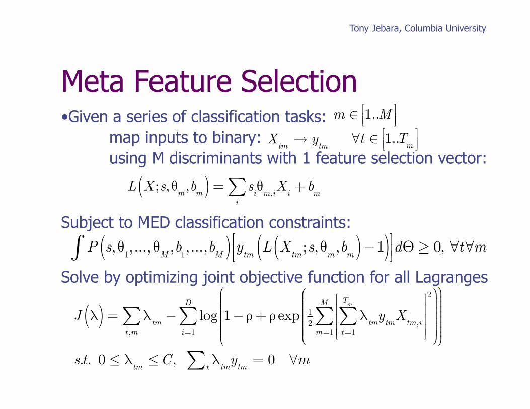
• Given a series of classification tasks: map inputs to binary: using M discriminants with 1 feature selection vector:
Subject to MED classification constraints:
Solve by optimizing joint objective function for all Lagranges
Meta Feature Selection m ∈ 1..M⎡⎣⎢
⎤⎦⎥
L X;s, θ
m,b
m( ) = siθ
m,iX
ii∑ +b
m
Xtm→ y
tm ∀t ∈ 1..T
m⎡⎣⎢
⎤⎦⎥
P s, θ
1,..., θ
M,b
1,...,b
M( ) ytm
L Xtm
;s, θm,b
m( )−1( )⎡⎣⎢
⎤⎦⎥∫ dΘ≥ 0, ∀t∀m
J λ( ) = λtm
t,m∑ − log 1−ρ+ ρ exp 1
2λ
tmy
tmX
tm,it=1
Tm
∑⎡
⎣
⎢⎢⎢
⎤
⎦
⎥⎥⎥m=1
M
∑2⎛
⎝
⎜⎜⎜⎜⎜⎜⎜
⎞
⎠
⎟⎟⎟⎟⎟⎟⎟⎟
⎛
⎝
⎜⎜⎜⎜⎜⎜⎜
⎞
⎠
⎟⎟⎟⎟⎟⎟⎟⎟i=1
D
∑
s.t. 0 ≤ λtm≤C, λ
tmy
tm= 0
t∑ ∀m
Tony Jebara, Columbia University
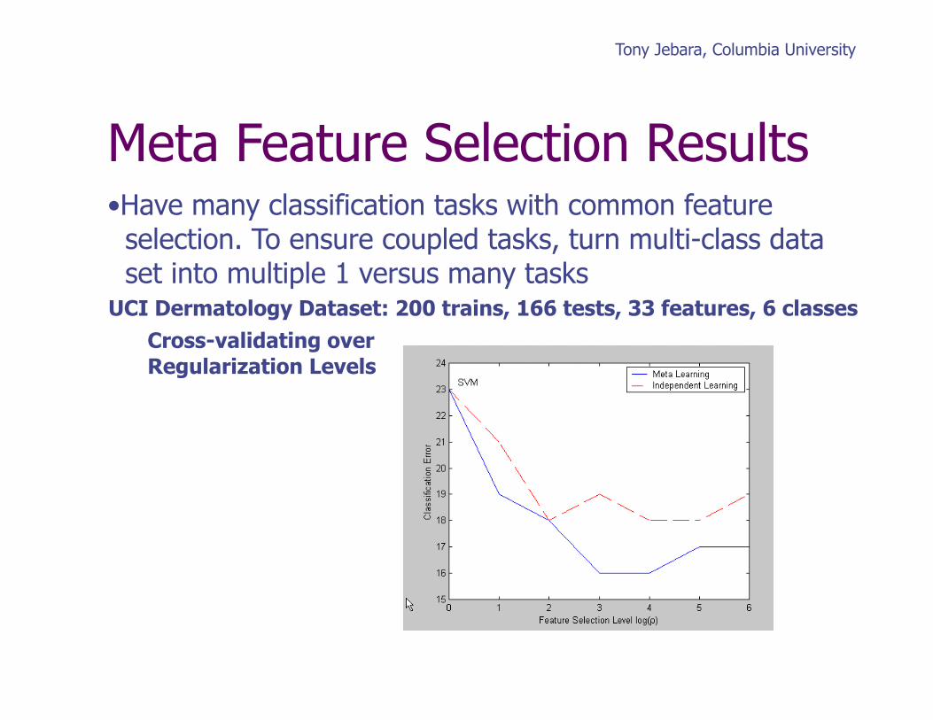
Meta Feature Selection Results
UCI Dermatology Dataset: 200 trains, 166 tests, 33 features, 6 classes Cross-validating over Regularization Levels
• Have many classification tasks with common feature selection. To ensure coupled tasks, turn multi-class data set into multiple 1 versus many tasks
Tony Jebara, Columbia University
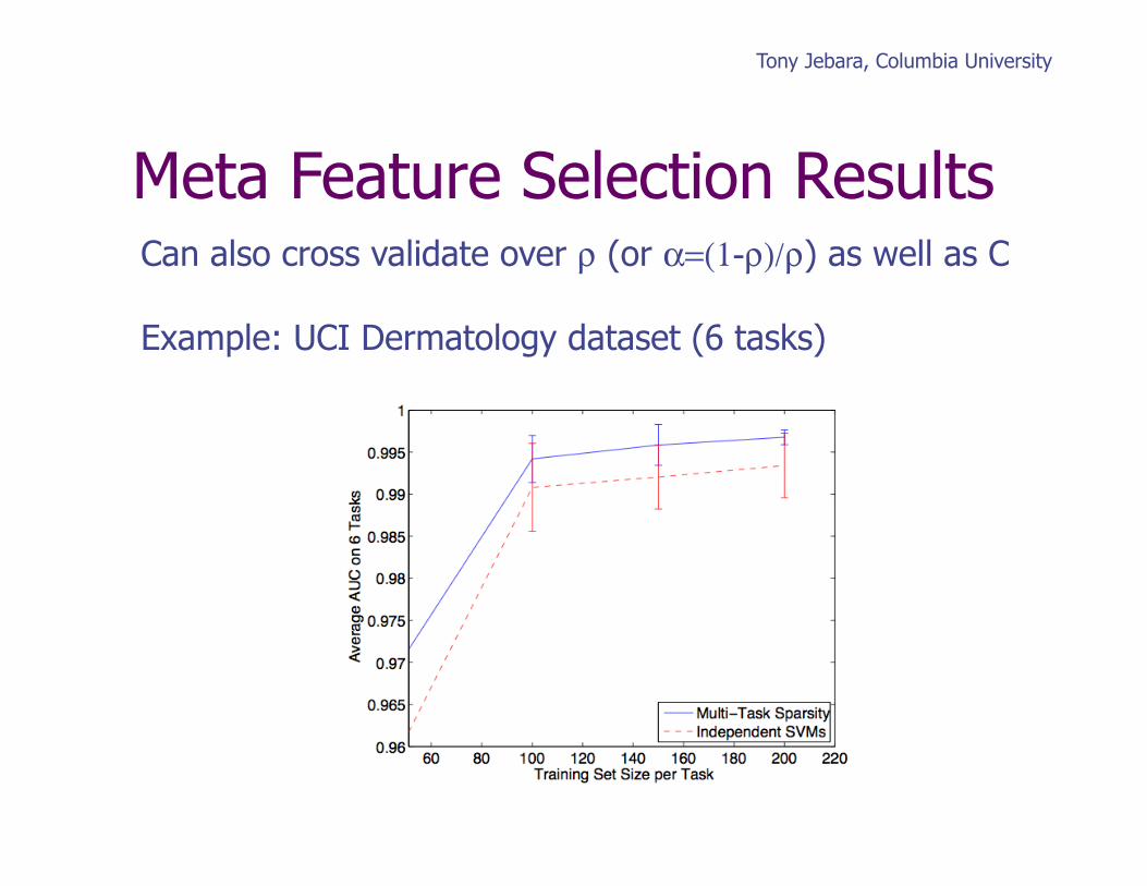
Meta Feature Selection Results Can also cross validate over ρ (or α=(1-ρ)/ρ) as well as C
Example: UCI Dermatology dataset (6 tasks)
Tony Jebara, Columbia University
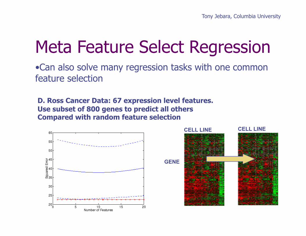
Meta Feature Select Regression
D. Ross Cancer Data: 67 expression level features. Use subset of 800 genes to predict all others Compared with random feature selection
GENE
CELL LINE CELL LINE
• Can also solve many regression tasks with one common feature selection
Tony Jebara, Columbia University
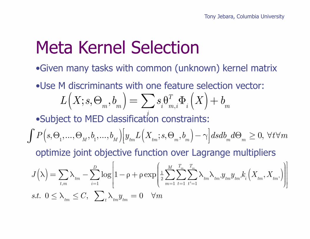
• Given many tasks with common (unknown) kernel matrix
• Use M discriminants with one feature selection vector:
• Subject to MED classification constraints:
optimize joint objective function over Lagrange multipliers
Meta Kernel Selection
L X;s,Θ
m,b
m( ) = siθ
m,iT Φ
iX( )
i∑ +b
m
P s,Θ
1,...,Θ
M,b
1,...,b
M( ) ytm
L Xtm
;s,Θm,b
m( )− γ⎡⎣⎢
⎤⎦⎥∫ dsdb
mdΘ
m≥ 0, ∀t∀m
J λ( ) = λtm
t,m∑ − log 1−ρ+ ρ exp 1
2λ
tmλ
tm 'y
tmy
tm 'k
iX
tm,X
tm '( )t '=1
Tm
∑t=1
Tm
∑m=1
M
∑⎛
⎝
⎜⎜⎜⎜⎜
⎞
⎠
⎟⎟⎟⎟⎟
⎡
⎣
⎢⎢⎢
⎤
⎦
⎥⎥⎥i=1
D
∑
s.t. 0 ≤ λtm≤C, λ
tmy
tm= 0
t∑ ∀m
Tony Jebara, Columbia University
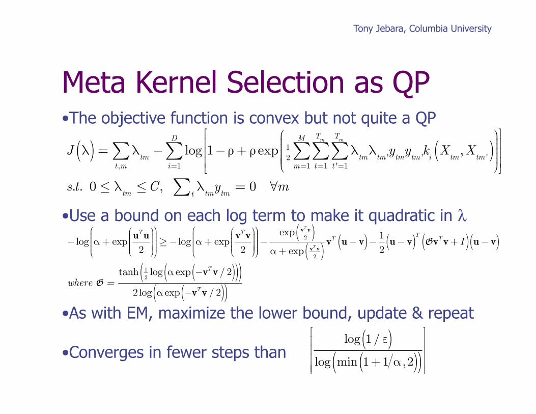
• The objective function is convex but not quite a QP
• Use a bound on each log term to make it quadratic in λ
• As with EM, maximize the lower bound, update & repeat
• Converges in fewer steps than
Meta Kernel Selection as QP
J λ( ) = λtm
t,m∑ − log 1−ρ+ ρ exp 1
2λ
tmλ
tm 'y
tmy
tm 'k
iX
tm,X
tm '( )t '=1
Tm
∑t=1
Tm
∑m=1
M
∑⎛
⎝
⎜⎜⎜⎜⎜
⎞
⎠
⎟⎟⎟⎟⎟
⎡
⎣
⎢⎢⎢
⎤
⎦
⎥⎥⎥i=1
D
∑
s.t. 0 ≤ λtm≤C, λ
tmy
tm= 0
t∑ ∀m
log 1/ ε( )log min 1 +1 α , 2( )( )⎡
⎢
⎢⎢⎢⎢
⎤
⎥
⎥⎥⎥⎥
− log α+ expuTu2
⎛
⎝⎜⎜⎜⎜
⎞
⎠⎟⎟⎟⎟⎟
⎛
⎝
⎜⎜⎜⎜
⎞
⎠
⎟⎟⎟⎟⎟≥− log α+ exp
vTv2
⎛
⎝⎜⎜⎜⎜
⎞
⎠⎟⎟⎟⎟⎟
⎛
⎝
⎜⎜⎜⎜
⎞
⎠
⎟⎟⎟⎟⎟−
exp vT v2( )
α+ exp vT v2( )
vT u− v( )− 12
u− v( )T GvTv + I( ) u− v( )
where G =tanh 1
2log α exp −vTv / 2( )( )( )
2 log α exp −vTv / 2( )( )
Tony Jebara, Columbia University
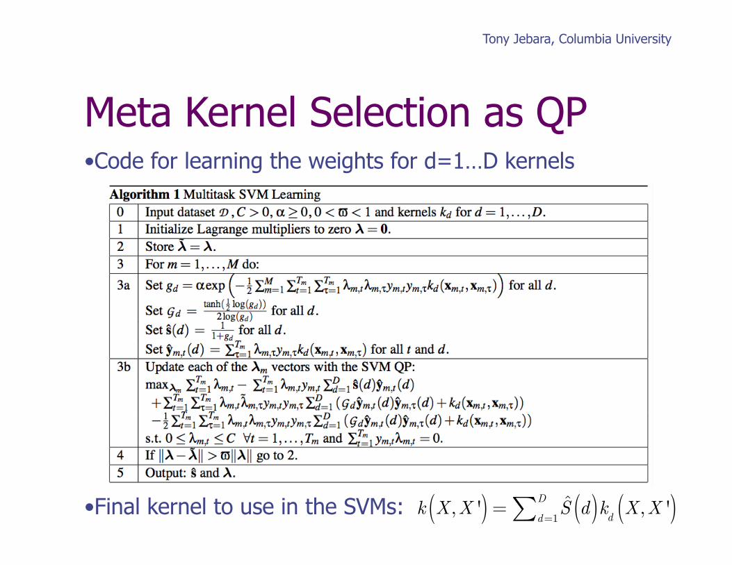
Meta Kernel Selection as QP • Code for learning the weights for d=1…D kernels
• Final kernel to use in the SVMs: k X,X '( ) = S d( )kd
X,X '( )d=1
D∑
Tony Jebara, Columbia University
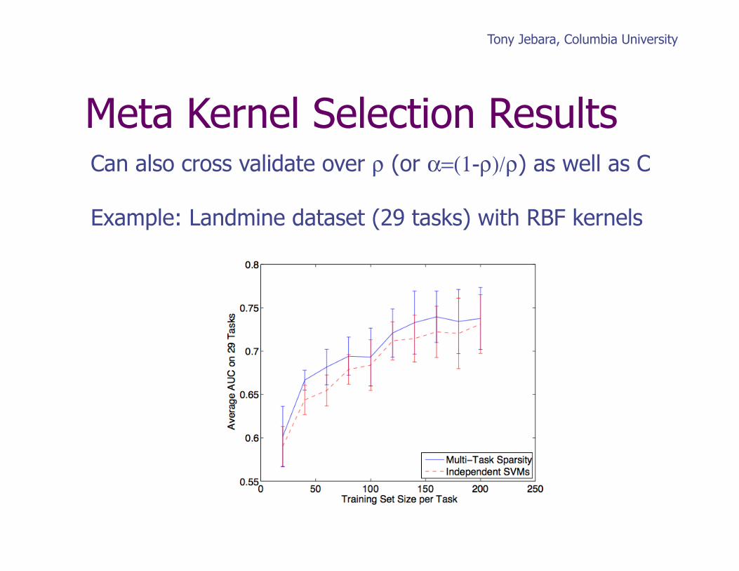
Meta Kernel Selection Results Can also cross validate over ρ (or α=(1-ρ)/ρ) as well as C
Example: Landmine dataset (29 tasks) with RBF kernels
Tony Jebara, Columbia University
Meta or Adaptive Pooling • Another type of meta-learning is adaptive pooling • Assume datasets predicting binary labels • Here, datasets are all labeled for the same task • But, inputs are sampled from slightly different distributions • E.g. Dataset 1: color face images labeled as male/female Dataset 2: gray face images labeled as male/female • Pooling: combine both datasets and learn one classifier
• Independent learning: learn a separate classifier for each
• Adaptive pooling: each classifier is a mix of the shared model and a specialized model
• Once again MED solution is straightforward…
L
mX( ) = θTX +b
m ∈ 1..M⎡⎣⎢
⎤⎦⎥
L
mX( ) = θ
mTX +b
m
L
mX( ) = s
mθ
mTX +b
m( ) + θTX +b( )

Tony Jebara, Columbia University
Meta or Adaptive Pooling • Compare to full pooling and independent learning
J λ( ) = λtm
t,m∑ − 1
2λ
tmλ
t 'm 'y
tmy
t 'm 'k X
tm,X
t 'm '( )t '=1
Tm
∑t=1
Tm
∑m '∑m∑
log α+ exp 12
λtmλ
tm 'y
tmy
tm 'k
mX
tm,X
tm '( )t '=1
Tm
∑t=1
Tm
∑⎛
⎝
⎜⎜⎜⎜⎜
⎞
⎠
⎟⎟⎟⎟⎟
⎡
⎣
⎢⎢⎢
⎤
⎦
⎥⎥⎥m=1
M
∑ + M log α+1( )
s.t. 0 ≤ λtm≤C, λ
tmy
tm= 0
t∑ ∀m