
Lecture5: StochasticHJBEquations, KolmogorovForwardEquations
35
Lecture 5: Stochastic HJB Equations, Kolmogorov Forward Equations ECO 521: Advanced Macroeconomics I Benjamin Moll Princeton University Fall 2012
Transcript of Lecture5: StochasticHJBEquations, KolmogorovForwardEquations
Lecture 5: Stochastic HJB Equations,Kolmogorov Forward Equations
ECO 521: Advanced Macroeconomics I
Benjamin Moll
Princeton University
Fall 2012
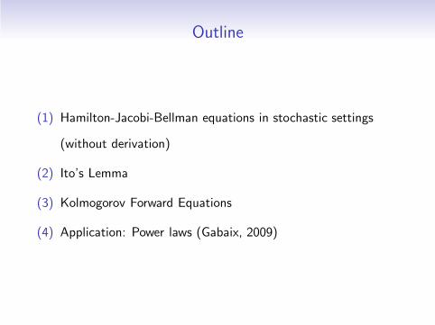
Outline
(1) Hamilton-Jacobi-Bellman equations in stochastic settings
(without derivation)
(2) Ito’s Lemma
(3) Kolmogorov Forward Equations
(4) Application: Power laws (Gabaix, 2009)
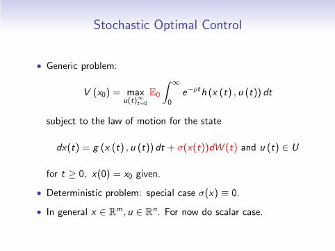
Stochastic Optimal Control
• Generic problem:
V (x0) = maxu(t)∞t=0
E0
∫
∞
0e−ρth (x (t) , u (t)) dt
subject to the law of motion for the state
dx(t) = g (x (t) , u (t)) dt + σ(x(t))dW (t) and u (t) ∈ U
for t ≥ 0, x(0) = x0 given.
• Deterministic problem: special case σ(x) ≡ 0.
• In general x ∈ Rm, u ∈ R
n. For now do scalar case.
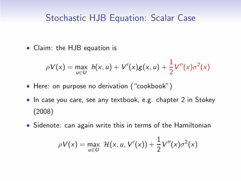
Stochastic HJB Equation: Scalar Case
• Claim: the HJB equation is
ρV (x) = maxu∈U
h(x , u) + V ′(x)g(x , u) +1
2V ′′(x)σ2(x)
• Here: on purpose no derivation (“cookbook”)
• In case you care, see any textbook, e.g. chapter 2 in Stokey
(2008)
• Sidenote: can again write this in terms of the Hamiltonian
ρV (x) = maxu∈U
H(x , u,V ′(x)) +1
2V ′′(x)σ2(x)
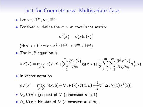
Just for Completeness: Multivariate Case
• Let x ∈ Rm, u ∈ R
n.
• For fixed x , define the m ×m covariance matrix
σ2(x) = σ(x)σ(x)′
(this is a function σ2 : Rm → Rm × R
m)
• The HJB equation is
ρV (x) = maxu∈U
h(x , u)+
m∑
i=1
∂V (x)
∂xigi (x , u)+
1
2
m∑
i=1
m∑
j=1
∂2V (x)
∂xi∂xjσ2ij(x)
• In vector notation
ρV (x) = maxu∈U
h(x , u)+∇xV (x)·g(x , u)+ 1
2tr(
∆xV (x)σ2(x))
• ∇xV (x): gradient of V (dimension m × 1)
• ∆xV (x): Hessian of V (dimension m ×m).
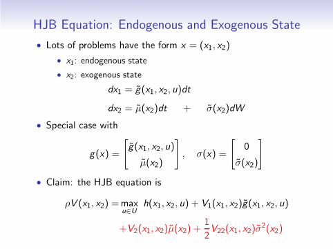
HJB Equation: Endogenous and Exogenous State
• Lots of problems have the form x = (x1, x2)
• x1: endogenous state
• x2: exogenous state
dx1 = g(x1, x2, u)dt
dx2 = µ(x2)dt + σ(x2)dW
• Special case with
g(x) =
[
g(x1, x2, u)
µ(x2)
]
, σ(x) =
[
0
σ(x2)
]
• Claim: the HJB equation is
ρV (x1, x2) =maxu∈U
h(x1, x2, u) + V1(x1, x2)g(x1, x2, u)
+V2(x1, x2)µ(x2) +1
2V22(x1, x2)σ
2(x2)
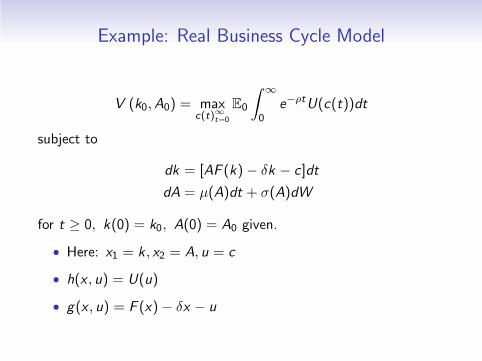
Example: Real Business Cycle Model
V (k0,A0) = maxc(t)∞t=0
E0
∫
∞
0e−ρtU(c(t))dt
subject to
dk = [AF (k)− δk − c]dt
dA = µ(A)dt + σ(A)dW
for t ≥ 0, k(0) = k0, A(0) = A0 given.
• Here: x1 = k , x2 = A, u = c
• h(x , u) = U(u)
• g(x , u) = F (x)− δx − u
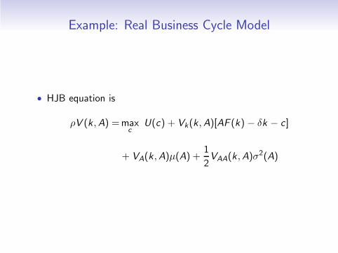
Example: Real Business Cycle Model
• HJB equation is
ρV (k ,A) =maxc
U(c) + Vk(k ,A)[AF (k) − δk − c]
+ VA(k ,A)µ(A) +1
2VAA(k ,A)σ
2(A)
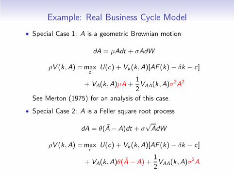
Example: Real Business Cycle Model
• Special Case 1: A is a geometric Brownian motion
dA = µAdt + σAdW
ρV (k ,A) =maxc
U(c) + Vk(k ,A)[AF (k) − δk − c]
+ VA(k ,A)µA +1
2VAA(k ,A)σ
2A2
See Merton (1975) for an analysis of this case.
• Special Case 2: A is a Feller square root process
dA = θ(A− A)dt + σ√AdW
ρV (k ,A) =maxc
U(c) + Vk(k ,A)[AF (k) − δk − c]
+ VA(k ,A)θ(A − A) +1
2VAA(k ,A)σ
2A
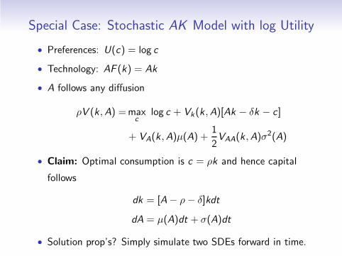
Special Case: Stochastic AK Model with log Utility
• Preferences: U(c) = log c
• Technology: AF (k) = Ak
• A follows any diffusion
ρV (k ,A) =maxc
log c + Vk(k ,A)[Ak − δk − c]
+ VA(k ,A)µ(A) +1
2VAA(k ,A)σ
2(A)
• Claim: Optimal consumption is c = ρk and hence capital
follows
dk = [A− ρ− δ]kdt
dA = µ(A)dt + σ(A)dt
• Solution prop’s? Simply simulate two SDEs forward in time.
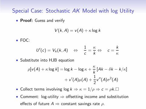
Special Case: Stochastic AK Model with log Utility
• Proof: Guess and verify
V (k ,A) = v(A) + κ log k
• FOC:
U ′(c) = Vk(k ,A) ⇔ 1
c=
κ
k⇔ c =
k
κ
• Substitute into HJB equation
ρ[v(A) + κ log k] = log k − log κ+κ
k[Ak − δk − k/κ]
+ v ′(A)µ(A) +1
2v ′′(A)σ2(A)
• Collect terms involving log k ⇒ κ = 1/ρ ⇒ c = ρk .�
• Comment: log-utility ⇒ offsetting income and substitution
effects of future A ⇒ constant savings rate ρ.
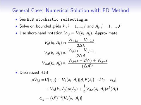
General Case: Numerical Solution with FD Method
• See HJB_stochastic_reflecting.m
• Solve on bounded grids ki , i = 1, ..., I and Aj , j = 1, ..., J
• Use short-hand notation Vi ,j = V (ki ,Aj). Approximate
Vk(ki ,Aj) ≈Vi+1,j − Vi−1,j
2∆k
VA(ki ,Aj) ≈Vi ,j+1 − Vi ,j+1
2∆A
VAA(ki ,Aj) ≈Vi ,j+1 − 2Vi ,j + Vi ,j−1
(∆A)2
• Discretized HJB
ρVi ,j =U(ci ,j) + Vk(ki ,Aj)[AjF (ki )− δki − ci ,j ]
+ VA(ki ,Aj)µ(Aj) +1
2VAA(ki ,Aj)σ
2(Aj)
ci ,j = (U ′)−1[Vk(ki ,Aj)]
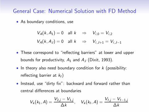
General Case: Numerical Solution with FD Method
• As boundary conditions, use
VA(k ,A1) = 0 all k ⇒ Vi ,0 = Vi ,2
VA(k ,AJ) = 0 all k ⇒ Vi ,J+1 = Vi ,J−1
• These correspond to “reflecting barriers” at lower and upper
bounds for productivity, A1 and AJ (Dixit, 1993).
• In theory also need boundary condition for k (possibility:
reflecting barrier at kI )
• Instead, use “dirty fix”: backward and forward rather than
central differences at boundaries
Vk(k1,A) =V2,j − V1,j
∆k, Vk(kI ,A) =
VI ,j − VI−1,j
∆k
General Case: Numerical Solution with FD Method
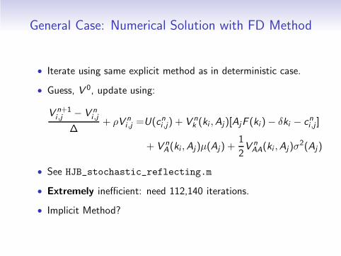
• Iterate using same explicit method as in deterministic case.
• Guess, V 0, update using:
V n+1i ,j − V n
i ,j
∆+ ρV n
i ,j =U(cni ,j) + V nk (ki ,Aj)[AjF (ki )− δki − cni ,j ]
+ V nA(ki ,Aj)µ(Aj) +
1
2V nAA(ki ,Aj)σ
2(Aj)
• See HJB_stochastic_reflecting.m
• Extremely inefficient: need 112,140 iterations.
• Implicit Method?
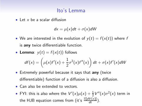
Ito’s Lemma
• Let x be a scalar diffusion
dx = µ(x)dt + σ(x)dW
• We are interested in the evolution of y(t) = f (x(t)) where f
is any twice differentiable function.
• Lemma: y(t) = f (x(t)) follows
df (x) =
(
µ(x)f ′(x) +1
2σ2(x)f ′′(x)
)
dt + σ(x)f ′(x)dW
• Extremely powerful because it says that any (twice
differentiable) function of a diffusion is also a diffusion.
• Can also be extended to vectors.
• FYI: this is also where the V ′(x)µ(x) + 12V
′′(x)σ2(x) term in
the HJB equation comes from (it’s E[dV (x)]dt
).
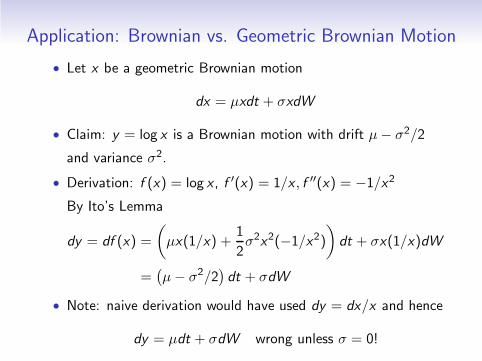
Application: Brownian vs. Geometric Brownian Motion
• Let x be a geometric Brownian motion
dx = µxdt + σxdW
• Claim: y = log x is a Brownian motion with drift µ− σ2/2
and variance σ2.
• Derivation: f (x) = log x , f ′(x) = 1/x , f ′′(x) = −1/x2
By Ito’s Lemma
dy = df (x) =
(
µx(1/x) +1
2σ2x2(−1/x2)
)
dt + σx(1/x)dW
=(
µ− σ2/2)
dt + σdW
• Note: naive derivation would have used dy = dx/x and hence
dy = µdt + σdW wrong unless σ = 0!
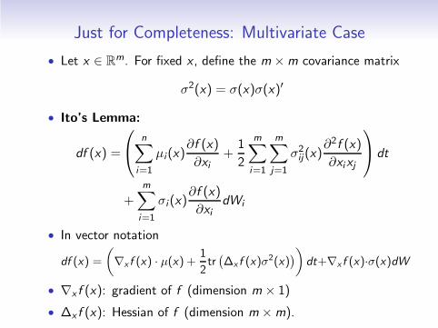
Just for Completeness: Multivariate Case
• Let x ∈ Rm. For fixed x , define the m ×m covariance matrix
σ2(x) = σ(x)σ(x)′
• Ito’s Lemma:
df (x) =
n∑
i=1
µi(x)∂f (x)
∂xi+
1
2
m∑
i=1
m∑
j=1
σ2ij(x)
∂2f (x)
∂xixj
dt
+m∑
i=1
σi (x)∂f (x)
∂xidWi
• In vector notation
df (x) =
(
∇x f (x) · µ(x) +1
2tr(
∆x f (x)σ2(x)
)
)
dt+∇x f (x)·σ(x)dW
• ∇x f (x): gradient of f (dimension m × 1)
• ∆x f (x): Hessian of f (dimension m ×m).
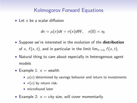
Kolmogorov Forward Equations
• Let x be a scalar diffusion
dx = µ(x)dt + σ(x)dW , x(0) = x0
• Suppose we’re interested in the evolution of the distribution
of x , f (x , t), and in particular in the limit limt→∞ f (x , t).
• Natural thing to care about especially in heterogenous agent
models
• Example 1: x = wealth
• µ(x) determined by savings behavior and return to investments
• σ(x) by return risk.
• microfound later
• Example 2: x = city size, will cover momentarily
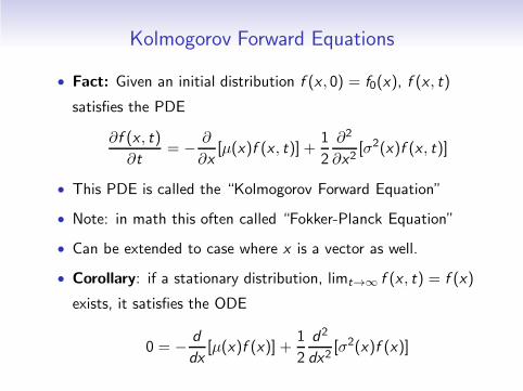
Kolmogorov Forward Equations
• Fact: Given an initial distribution f (x , 0) = f0(x), f (x , t)
satisfies the PDE
∂f (x , t)
∂t= − ∂
∂x[µ(x)f (x , t)] +
1
2
∂2
∂x2[σ2(x)f (x , t)]
• This PDE is called the “Kolmogorov Forward Equation”
• Note: in math this often called “Fokker-Planck Equation”
• Can be extended to case where x is a vector as well.
• Corollary: if a stationary distribution, limt→∞ f (x , t) = f (x)
exists, it satisfies the ODE
0 = − d
dx[µ(x)f (x)] +
1
2
d2
dx2[σ2(x)f (x)]
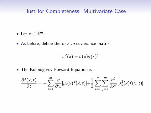
Just for Completeness: Multivariate Case
• Let x ∈ Rm.
• As before, define the m ×m covariance matrix
σ2(x) = σ(x)σ(x)′
• The Kolmogorov Forward Equation is
∂f (x , t)
∂t= −
m∑
i=1
∂
∂xi[µi(x)f (x , t)]+
1
2
m∑
i=1
m∑
j=1
∂2
∂x2[σ2
ij(x)f (x , t)]
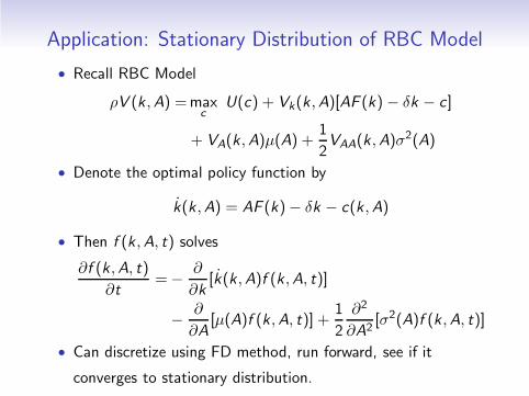
Application: Stationary Distribution of RBC Model
• Recall RBC Model
ρV (k ,A) =maxc
U(c) + Vk(k ,A)[AF (k) − δk − c]
+ VA(k ,A)µ(A) +1
2VAA(k ,A)σ
2(A)
• Denote the optimal policy function by
k(k ,A) = AF (k)− δk − c(k ,A)
• Then f (k ,A, t) solves
∂f (k ,A, t)
∂t=− ∂
∂k[k(k ,A)f (k ,A, t)]
− ∂
∂A[µ(A)f (k ,A, t)] +
1
2
∂2
∂A2[σ2(A)f (k ,A, t)]
• Can discretize using FD method, run forward, see if it
converges to stationary distribution.
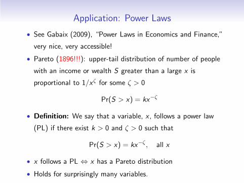
Application: Power Laws
• See Gabaix (2009), “Power Laws in Economics and Finance,”
very nice, very accessible!
• Pareto (1896!!!): upper-tail distribution of number of people
with an income or wealth S greater than a large x is
proportional to 1/xζ for some ζ > 0
Pr(S > x) = kx−ζ
• Definition: We say that a variable, x , follows a power law
(PL) if there exist k > 0 and ζ > 0 such that
Pr(S > x) = kx−ζ , all x
• x follows a PL ⇔ x has a Pareto distribution
• Holds for surprisingly many variables.
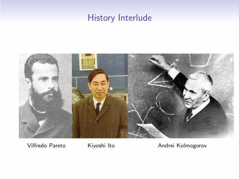
History Interlude
Vilfredo Pareto Kiyoshi Ito Andrei Kolmogorov
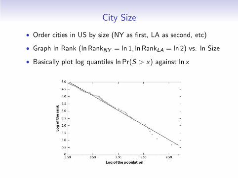
City Size
• Order cities in US by size (NY as first, LA as second, etc)
• Graph ln Rank (ln RankNY = ln 1, ln RankLA = ln 2) vs. ln Size
• Basically plot log quantiles ln Pr(S > x) against ln x
City Size
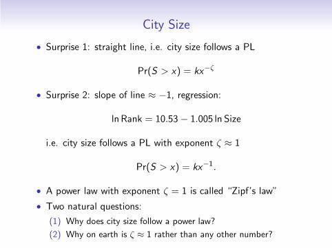
• Surprise 1: straight line, i.e. city size follows a PL
Pr(S > x) = kx−ζ
• Surprise 2: slope of line ≈ −1, regression:
ln Rank = 10.53 − 1.005 ln Size
i.e. city size follows a PL with exponent ζ ≈ 1
Pr(S > x) = kx−1.
• A power law with exponent ζ = 1 is called “Zipf’s law”
• Two natural questions:
(1) Why does city size follow a power law?
(2) Why on earth is ζ ≈ 1 rather than any other number?
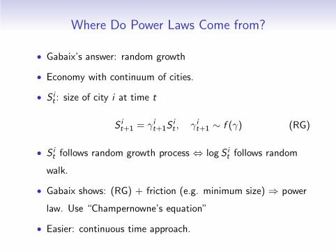
Where Do Power Laws Come from?
• Gabaix’s answer: random growth
• Economy with continuum of cities.
• S it : size of city i at time t
S it+1 = γit+1S
it , γit+1 ∼ f (γ) (RG)
• S it follows random growth process ⇔ log S i
t follows random
walk.
• Gabaix shows: (RG) + friction (e.g. minimum size) ⇒ power
law. Use “Champernowne’s equation”
• Easier: continuous time approach.
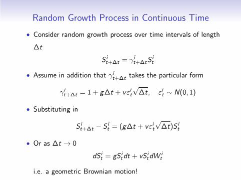
Random Growth Process in Continuous Time
• Consider random growth process over time intervals of length
∆t
S it+∆t = γit+∆tS
it
• Assume in addition that γit+∆t takes the particular form
γit+∆t = 1 + g∆t + vεit√∆t, εit ∼ N(0, 1)
• Substituting in
S it+∆t − S i
t = (g∆t + vεit√∆t)S i
t
• Or as ∆t → 0
dS it = gS i
tdt + vS itdW
it
i.e. a geometric Brownian motion!
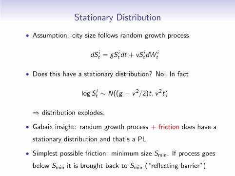
Stationary Distribution
• Assumption: city size follows random growth process
dS it = gS i
tdt + vS itdW
it
• Does this have a stationary distribution? No! In fact
log S it ∼ N((g − v2/2)t, v2t)
⇒ distribution explodes.
• Gabaix insight: random growth process + friction does have a
stationary distribution and that’s a PL
• Simplest possible friction: minimum size Smin. If process goes
below Smin it is brought back to Smin (“reflecting barrier”)
Stationary Distribution
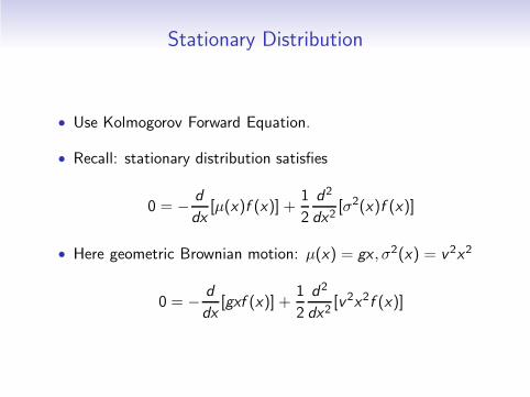
• Use Kolmogorov Forward Equation.
• Recall: stationary distribution satisfies
0 = − d
dx[µ(x)f (x)] +
1
2
d2
dx2[σ2(x)f (x)]
• Here geometric Brownian motion: µ(x) = gx , σ2(x) = v2x2
0 = − d
dx[gxf (x)] +
1
2
d2
dx2[v2x2f (x)]
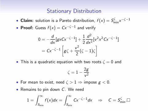
Stationary Distribution
• Claim: solution is a Pareto distribution, f (x) = Sζminx
−ζ−1
• Proof: Guess f (x) = Cx−ζ−1 and verify
0 = − d
dx[gxCx−ζ−1] +
1
2
d2
dx2[v2x2Cx−ζ−1]
= Cx−ζ−1
[
gζ +v2
2(ζ − 1)ζ
]
• This is a quadratic equation with two roots ζ = 0 and
ζ = 1− 2g
v2
• For mean to exist, need ζ > 1 ⇒ impose g < 0.
• Remains to pin down C . We need
1 =
∫
∞
Smin
f (x)dx =
∫
∞
Smin
Cx−ζ−1dx ⇒ C = Sζmin.�
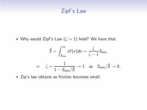
Zipf’s Law
• Why would Zipf’s Law (ζ = 1) hold? We have that
S =
∫
∞
Smin
xf (x)dx =ζ
ζ − 1Smin
⇒ ζ =1
1− Smin/S→ 1 as Smin/S → 0.
• Zip’s law obtains as friction becomes small.
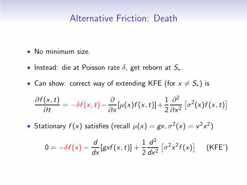
Alternative Friction: Death
• No minimum size.
• Instead: die at Poisson rate δ, get reborn at S∗.
• Can show: correct way of extending KFE (for x 6= S∗) is
∂f (x , t)
∂t= −δf (x , t)− ∂
∂x[µ(x)f (x , t)]+
1
2
∂2
∂x2[
σ2(x)f (x , t)]
• Stationary f (x) satisfies (recall µ(x) = gx , σ2(x) = v2x2)
0 = −δf (x) − d
dx[gxf (x , t)] +
1
2
d2
dx2
[
σ2x2f (x)]
(KFE’)
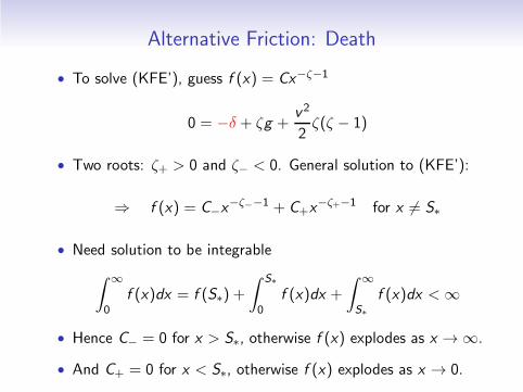
Alternative Friction: Death
• To solve (KFE’), guess f (x) = Cx−ζ−1
0 = −δ + ζg +v2
2ζ(ζ − 1)
• Two roots: ζ+ > 0 and ζ− < 0. General solution to (KFE’):
⇒ f (x) = C−x−ζ−−1 + C+x
−ζ+−1 for x 6= S∗
• Need solution to be integrable
∫
∞
0f (x)dx = f (S∗) +
∫ S∗
0f (x)dx +
∫
∞
S∗
f (x)dx < ∞
• Hence C− = 0 for x > S∗, otherwise f (x) explodes as x → ∞.
• And C+ = 0 for x < S∗, otherwise f (x) explodes as x → 0.
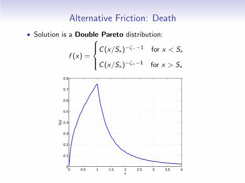
Alternative Friction: Death
• Solution is a Double Pareto distribution:
f (x) =
C (x/S∗)−ζ−−1 for x < S∗
C (x/S∗)−ζ+−1 for x > S∗
0 0.5 1 1.5 2 2.5 3 3.5 40
0.1
0.2
0.3
0.4
0.5
0.6
0.7
0.8
x
f(x)
Alternative Friction: Death
• Again, Zipf’s Law (ζ = 1) obtains as friction gets small.
Here: δ → 0.
• Other cases in Gabaix’s paper:
(1) Extension to jump processes
(2) Approximate power laws with generalized growth process
dSt
St= g(St)dt + v(St)dt


![Lecture 5: Variance Reduction - LAGA - Accueilkebaier/Lecture5.pdfAntithetic Variables Antithetic Variables Assume that we aim at computing ˇ= E(g(U)), where U ˘U([0;1]): We simulate](https://static.fdocument.org/doc/165x107/5f8dc882f6ffaa497a7a5af9/lecture-5-variance-reduction-laga-accueil-kebaierlecture5pdf-antithetic-variables.jpg)