Lecture 8THE AGGREGATE EXPENDITURE

MODEL

A STYLIZED LOOK AT

BUSINESS CYCLE DYNAMICS

September 25th 2019

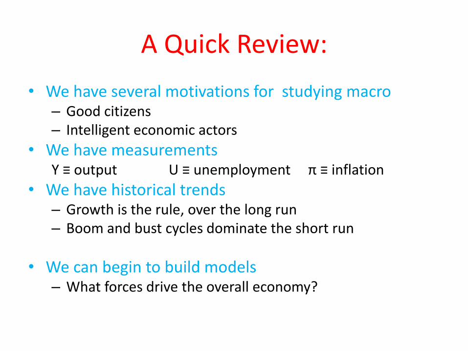
A Quick Review:

• We have several motivations for studying macro – Good citizens– Intelligent economic actors

• We have measurementsY ≡ output U ≡ unemployment π ≡ inflation

• We have historical trends– Growth is the rule, over the long run– Boom and bust cycles dominate the short run

• We can begin to build models– What forces drive the overall economy?

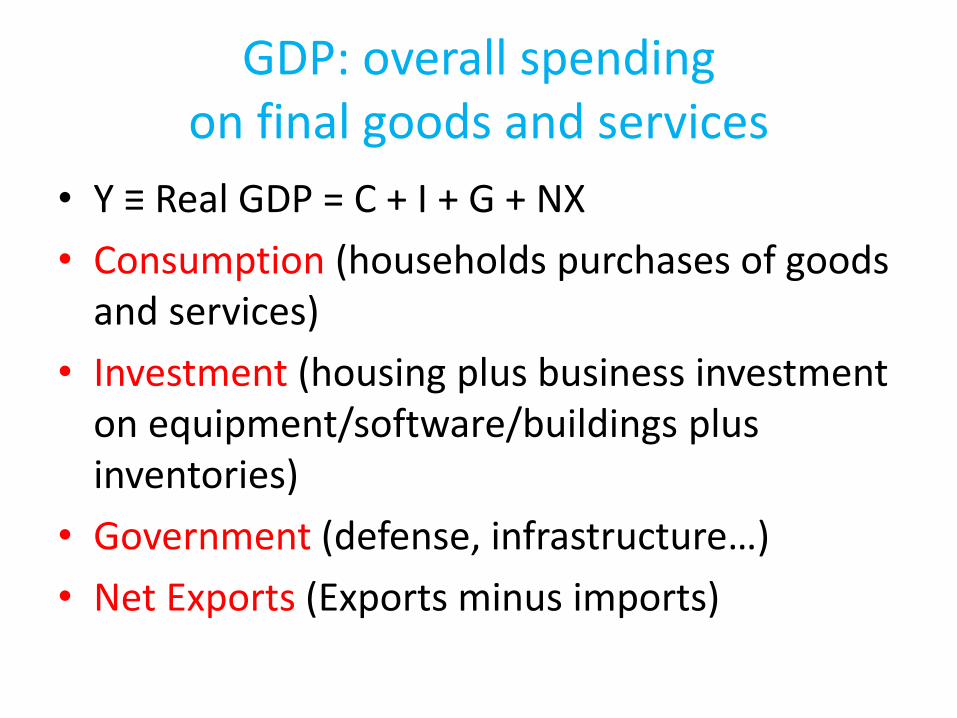
GDP: overall spending on final goods and services

• Y ≡ Real GDP = C + I + G + NX

• Consumption (households purchases of goods and services)

• Investment (housing plus business investment on equipment/software/buildings plus inventories)

• Government (defense, infrastructure…)

• Net Exports (Exports minus imports)

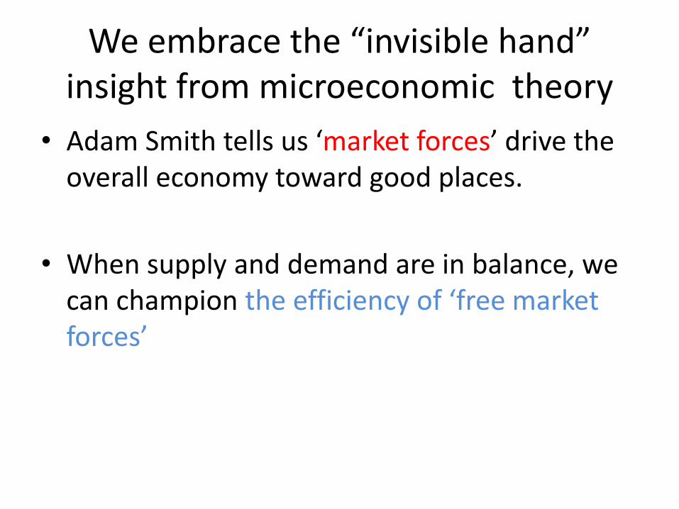
We embrace the “invisible hand” insight from microeconomic theory

• Adam Smith tells us ‘market forces’ drive the overall economy toward good places.

• When supply and demand are in balance, we can champion the efficiency of ‘free market forces’

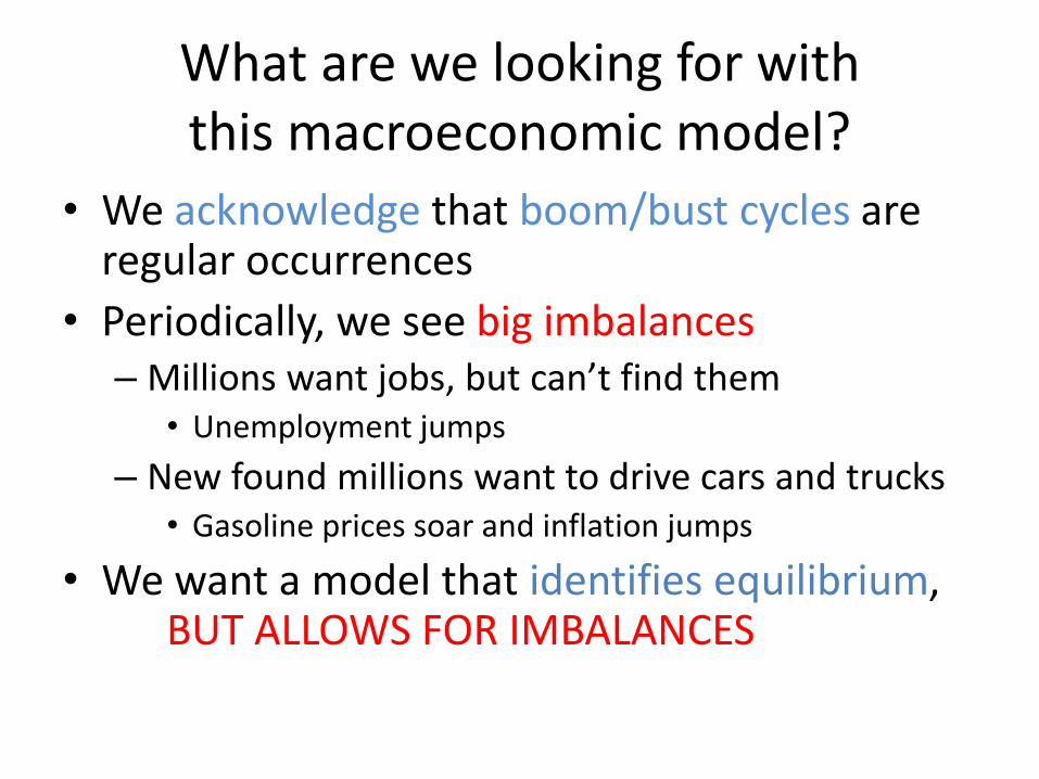
What are we looking for with this macroeconomic model?

• We acknowledge that boom/bust cycles are regular occurrences

• Periodically, we see big imbalances– Millions want jobs, but can’t find them

• Unemployment jumps

– New found millions want to drive cars and trucks• Gasoline prices soar and inflation jumps

• We want a model that identifies equilibrium,BUT ALLOWS FOR IMBALANCES

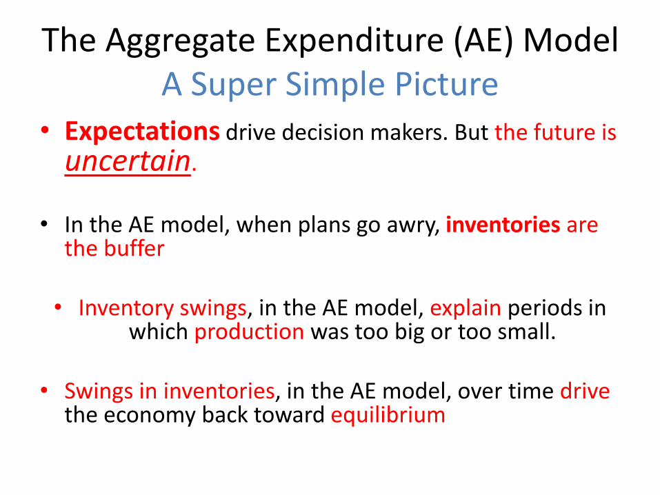
The Aggregate Expenditure (AE) ModelA Super Simple Picture

• Expectations drive decision makers. But the future is uncertain.

• In the AE model, when plans go awry, inventories are the buffer

• Inventory swings, in the AE model, explain periods in which production was too big or too small.

• Swings in inventories, in the AE model, over time drivethe economy back toward equilibrium

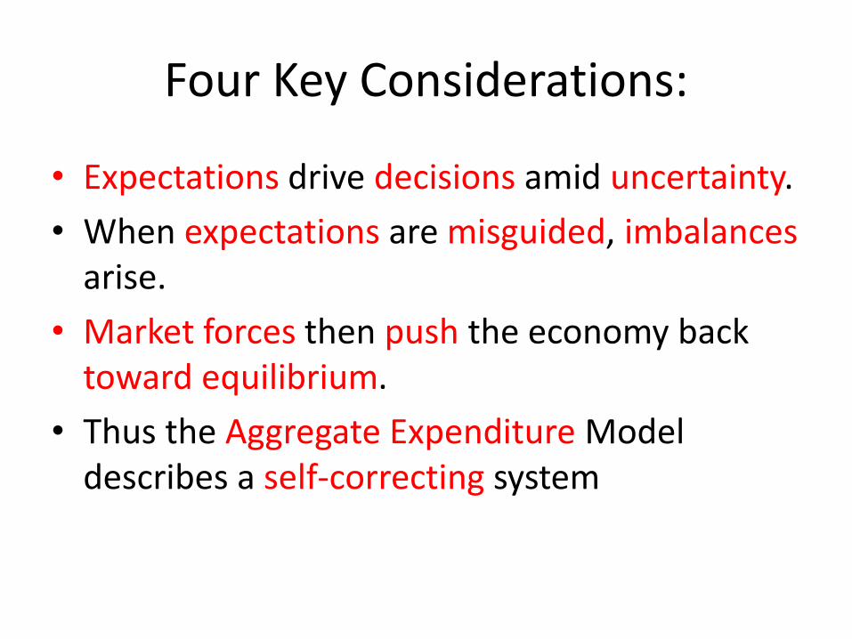
Four Key Considerations:

• Expectations drive decisions amid uncertainty.

• When expectations are misguided, imbalancesarise.

• Market forces then push the economy back toward equilibrium.

• Thus the Aggregate Expenditure Model describes a self-correcting system

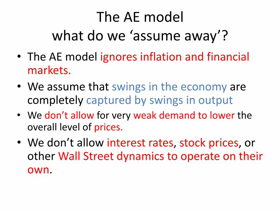
The AE modelwhat do we ‘assume away’?

• The AE model ignores inflation and financial markets.

• We assume that swings in the economy are completely captured by swings in output

• We don’t allow for very weak demand to lower the overall level of prices.

• We don’t allow interest rates, stock prices, or other Wall Street dynamics to operate on their own.

The AE Model: SummingAggregate Expenditures

AE = C + I + G + NXC = Consumption

I = Planned Investment

G = Government

NX = net exports

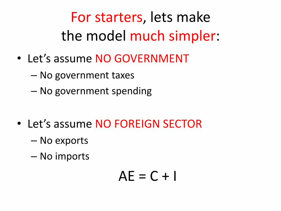
For starters, lets make the model much simpler:

• Let’s assume NO GOVERNMENT

– No government taxes

– No government spending

• Let’s assume NO FOREIGN SECTOR

– No exports

– No imports

AE = C + I

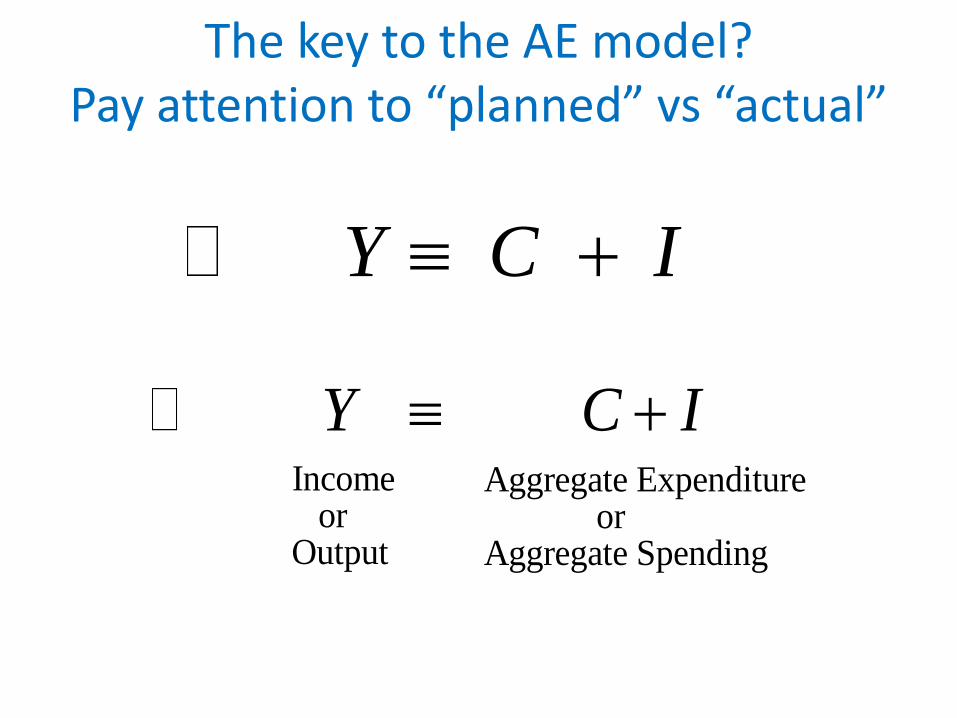
The key to the AE model?Pay attention to “planned” vs “actual”

Y C I +

Income Aggregate Expenditure or orOutput Aggregate Spending

Y C I +

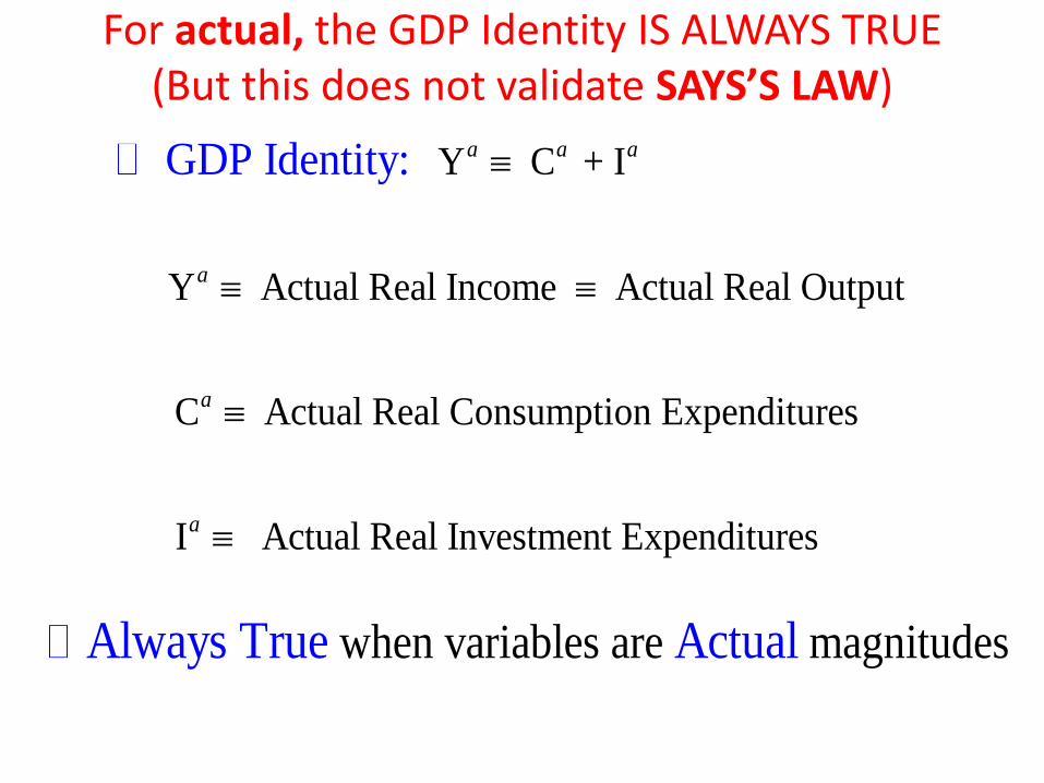
For actual, the GDP Identity IS ALWAYS TRUE(But this does not validate SAYS’S LAW)

Y C + I

Y Actual Real Income Actual Real Output

C Actual Real Consumption Expenditures

I Actual Real Investment Expenditures

GDP Identity: a a a

a

a

a

when variables are magn tudes iAlways True Actual

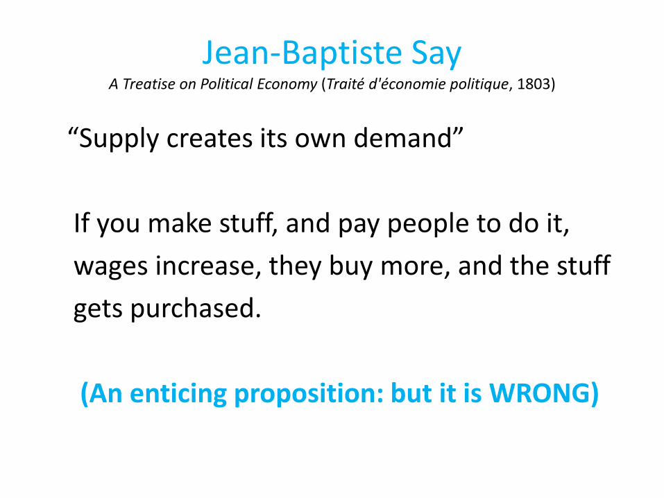
Jean-Baptiste SayA Treatise on Political Economy (Traité d'économie politique, 1803)

“Supply creates its own demand”

If you make stuff, and pay people to do it,

wages increase, they buy more, and the stuff

gets purchased.

(An enticing proposition: but it is WRONG)

Y = C + I

Y Planned Real Income Planned Real Output

C Planned Real Consumption Expenditures

I Planned Real Investment Expenditures

Equilibrium Condition:

Continuedp p p

p

p

p

in when variables are

magnitudes

Only True Equilibrium Planned

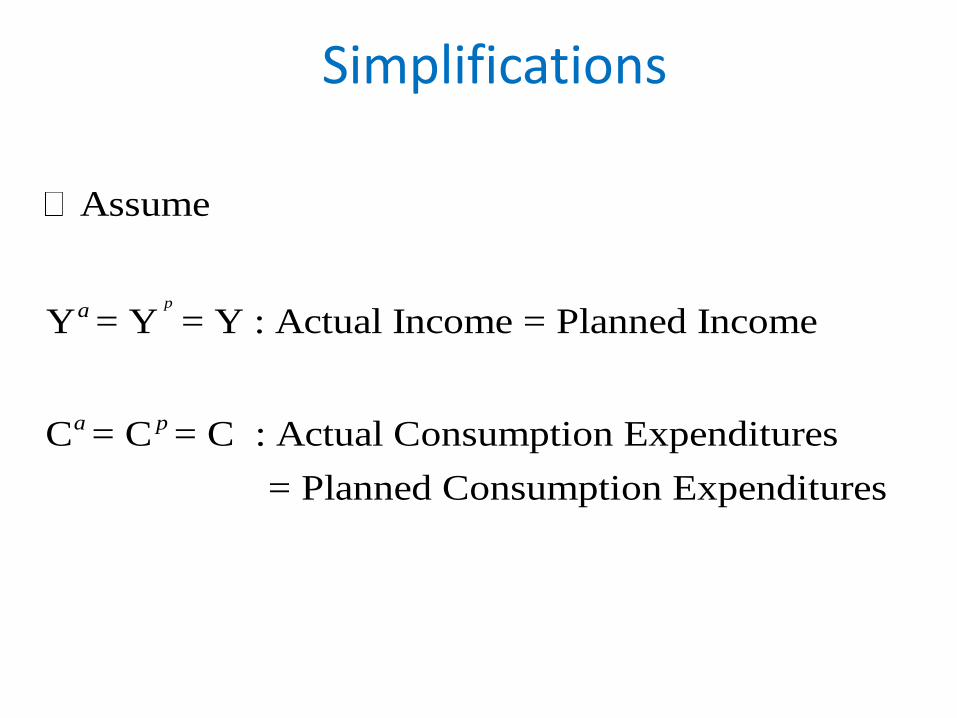
Assume

Y = Y = Y : Actual Income = Planned Income

C = C = C : Actual Consumption Expenditures

= Planned Consumption Expenditures

pa

a p

Simplifications

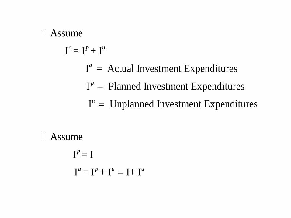
Assume

I = I + I

I = Actual Investment Expenditures

I Planned Investment Expenditures

I Unplanned Investment Expenditures

Assume

I = I

I = I + I I+ I

a p u

a

p

u

p

a p u u

=

=

=

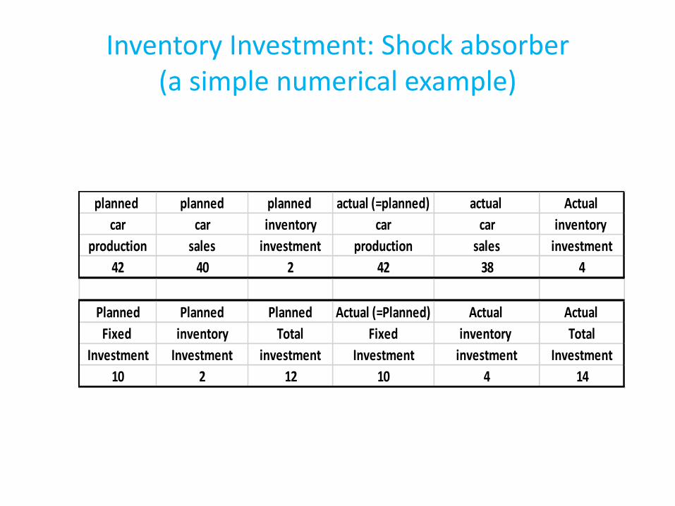
Inventory Investment: Shock absorber(a simple numerical example)

planned planned planned actual (=planned) actual Actual

car car inventory car car inventory

production sales investment production sales investment

42 40 2 42 38 4

Planned Planned Planned Actual (=Planned) Actual Actual

Fixed inventory Total Fixed inventory Total

Investment Investment investment Investment investment Investment

10 2 12 10 4 14

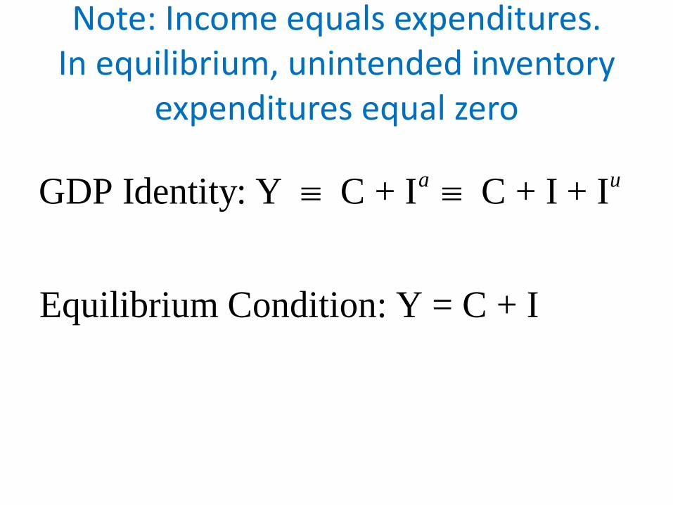
Note: Income equals expenditures.In equilibrium, unintended inventory

expenditures equal zero

GDP Identity: Y C + I C + I + I

Equilibrium Condition: Y = C + I

a u

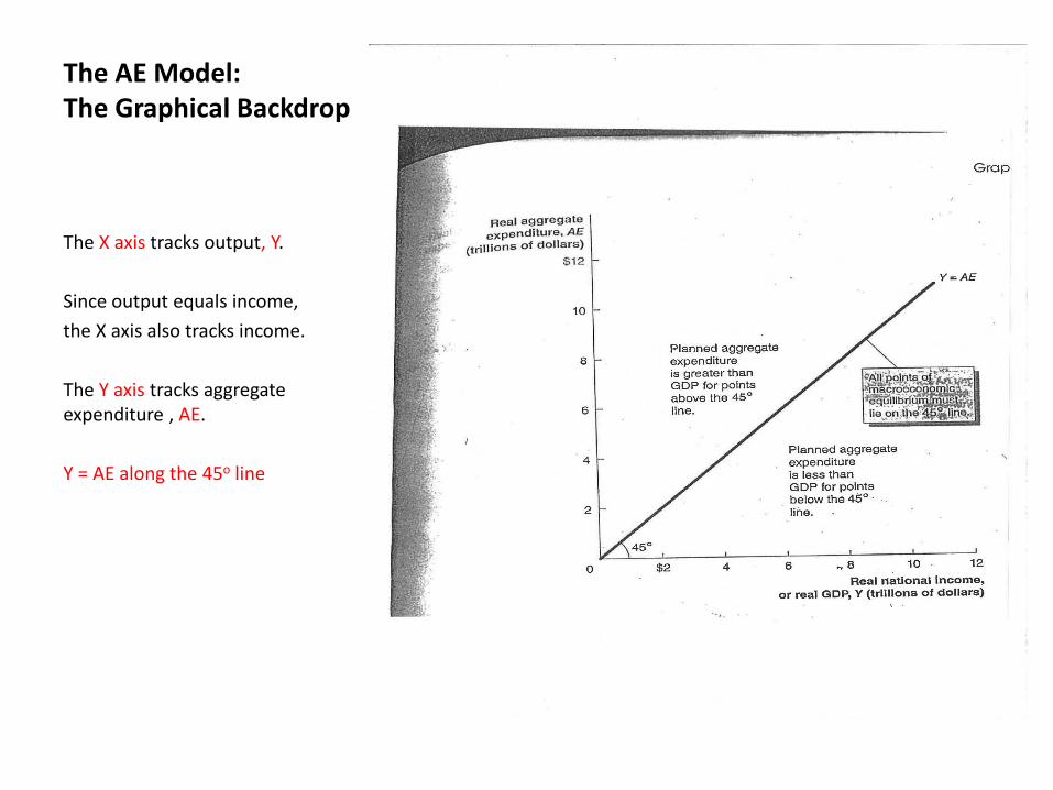
The AE Model:The Graphical Backdrop

The X axis tracks output, Y.

Since output equals income,

the X axis also tracks income.

The Y axis tracks aggregate expenditure , AE.

Y = AE along the 45o line

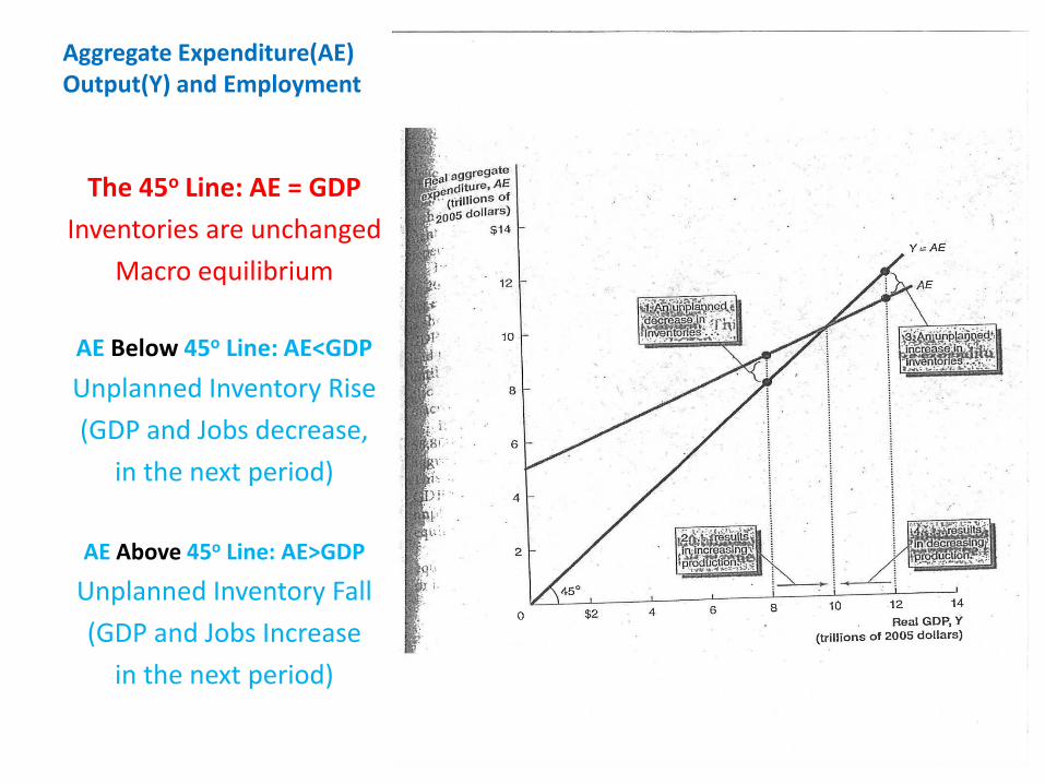
Aggregate Expenditure(AE)Output(Y) and Employment

The 45o Line: AE = GDP

Inventories are unchanged

Macro equilibrium

AE Below 45o Line: AE<GDP

Unplanned Inventory Rise

(GDP and Jobs decrease,

in the next period)

AE Above 45o Line: AE>GDP

Unplanned Inventory Fall

(GDP and Jobs Increase

in the next period)

The AE Model: An Equilibrium Seeking Framework

• Supply/demand charts, in microeconomics. We imagine shifts toward equilibrium price.

• AE Model, with inventory swings, provide a storyline for system that seeks equilibrium.

• When we introduce Wall Street, we discover forces that, at times, DON’T PUSH US TOWARD EQUILIBRIUM: ADVERSE FEEDBACK LOOPS

What Drives AEComponents?

What key variables explain swings in

C ≡ consumption

I ≡ Investment

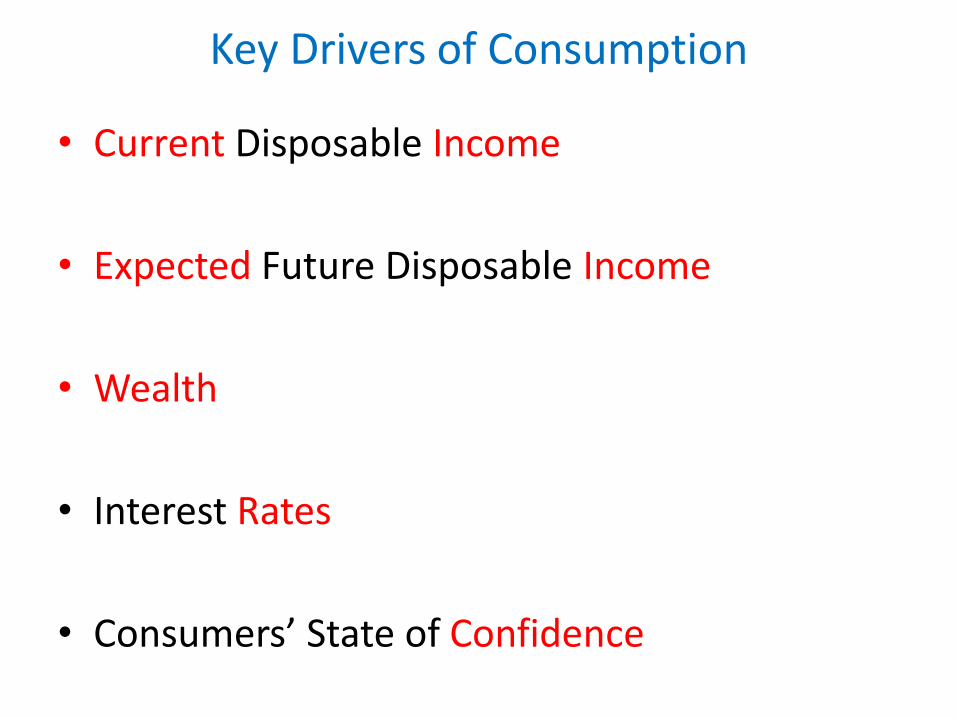
Key Drivers of Consumption

• Current Disposable Income

• Expected Future Disposable Income

• Wealth

• Interest Rates

• Consumers’ State of Confidence

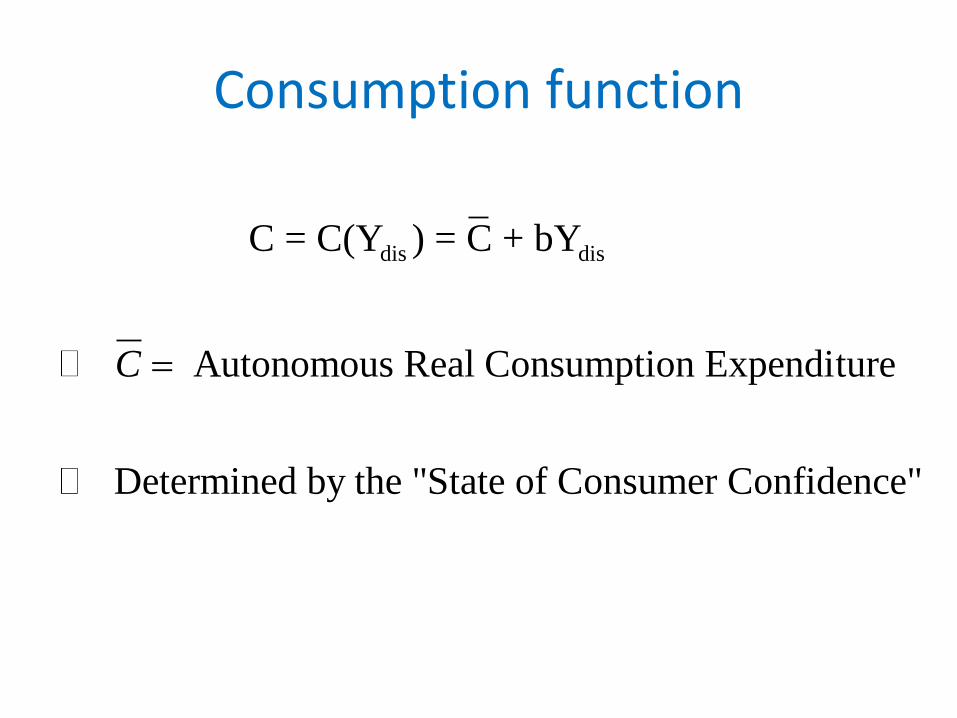
Consumption function

dis dis C = C(Y ) = C + bY

Autonomous Real Consumption Expenditure

Determined by the "State of Consumer Confidence"

C =

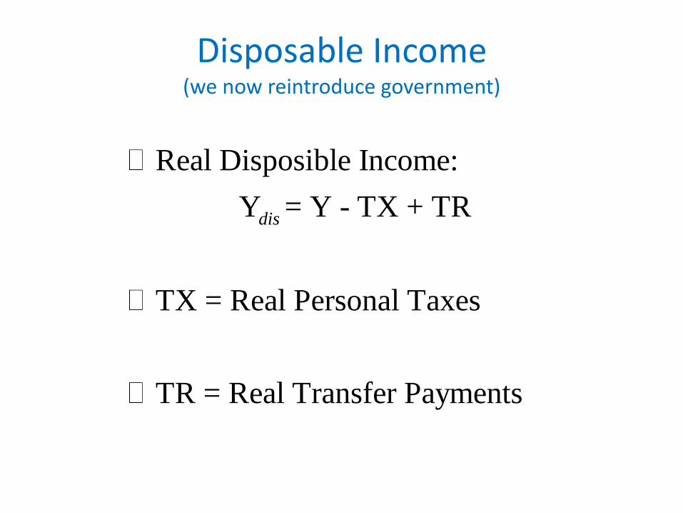
Disposable Income(we now reintroduce government)

Real Disposible Income:

Y = Y - TX + TR

TX = Real Personal Taxes

TR = Real Transfer Payments

dis

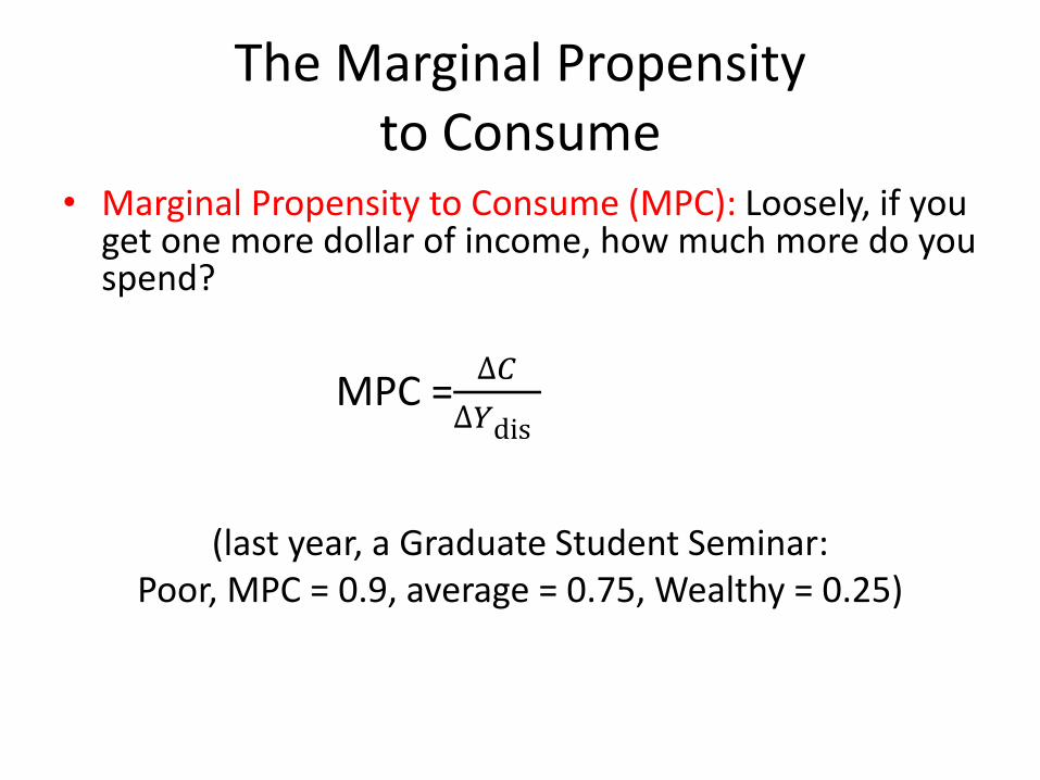
The Marginal Propensity to Consume

• Marginal Propensity to Consume (MPC): Loosely, if you get one more dollar of income, how much more do you spend?

MPC =∆𝐶

∆𝑌dis

(last year, a Graduate Student Seminar:Poor, MPC = 0.9, average = 0.75, Wealthy = 0.25)

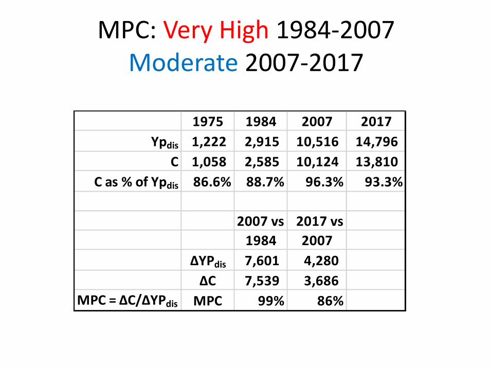
MPC: Very High 1984-2007Moderate 2007-2017

1975 1984 2007 2017

Ypdis 1,222 2,915 10,516 14,796

C 1,058 2,585 10,124 13,810

C as % of Ypdis 86.6% 88.7% 96.3% 93.3%

2007 vs 2017 vs

1984 2007

ΔYPdis 7,601 4,280

ΔC 7,539 3,686

MPC = ΔC/ΔYPdis MPC 99% 86%

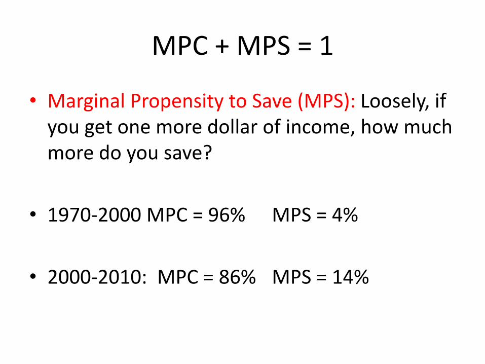
MPC + MPS = 1

• Marginal Propensity to Save (MPS): Loosely, if you get one more dollar of income, how much more do you save?

• 1970-2000 MPC = 96% MPS = 4%

• 2000-2010: MPC = 86% MPS = 14%

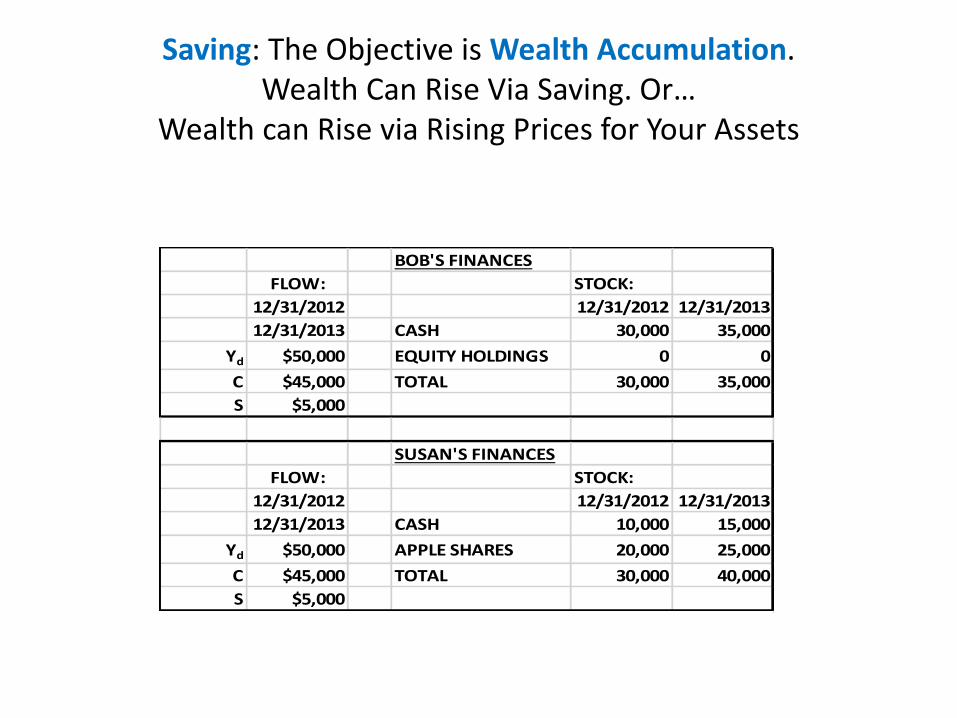
Saving: The Objective is Wealth Accumulation. Wealth Can Rise Via Saving. Or…

Wealth can Rise via Rising Prices for Your Assets

BOB'S FINANCES

FLOW: STOCK:

12/31/2012 12/31/2012 12/31/2013

12/31/2013 CASH 30,000 35,000

Yd $50,000 EQUITY HOLDINGS 0 0

C $45,000 TOTAL 30,000 35,000

S $5,000

SUSAN'S FINANCES

FLOW: STOCK:

12/31/2012 12/31/2012 12/31/2013

12/31/2013 CASH 10,000 15,000

Yd $50,000 APPLE SHARES 20,000 25,000

C $45,000 TOTAL 30,000 40,000

S $5,000

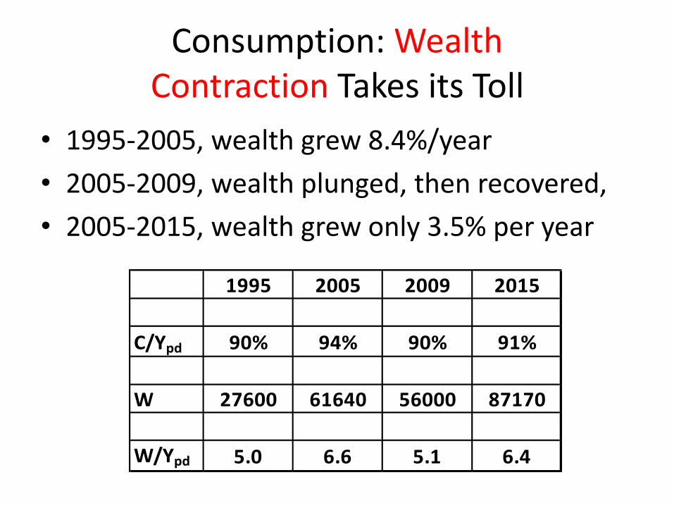
Consumption: WealthContraction Takes its Toll

• 1995-2005, wealth grew 8.4%/year

• 2005-2009, wealth plunged, then recovered,

• 2005-2015, wealth grew only 3.5% per year

1995 2005 2009 2015

C/Ypd 90% 94% 90% 91%

W 27600 61640 56000 87170

W/Ypd 5.0 6.6 5.1 6.4

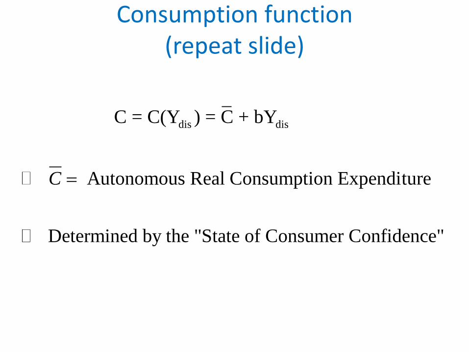
Consumption function(repeat slide)

dis dis C = C(Y ) = C + bY

Autonomous Real Consumption Expenditure

Determined by the "State of Consumer Confidence"

C =

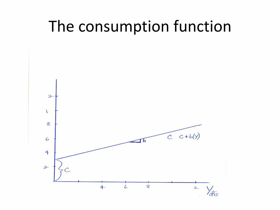
The consumption function

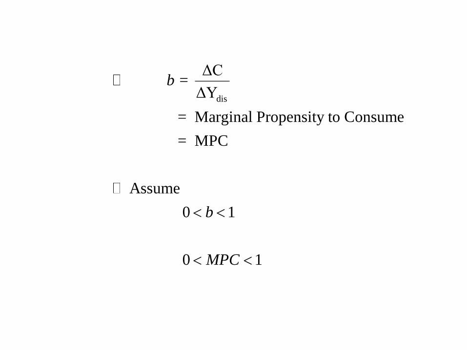
dis

ΔC =

ΔY

= Marginal Propensity to Consume

= MPC

Assume

0 1

0 1

b

b

MPC

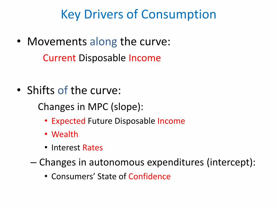
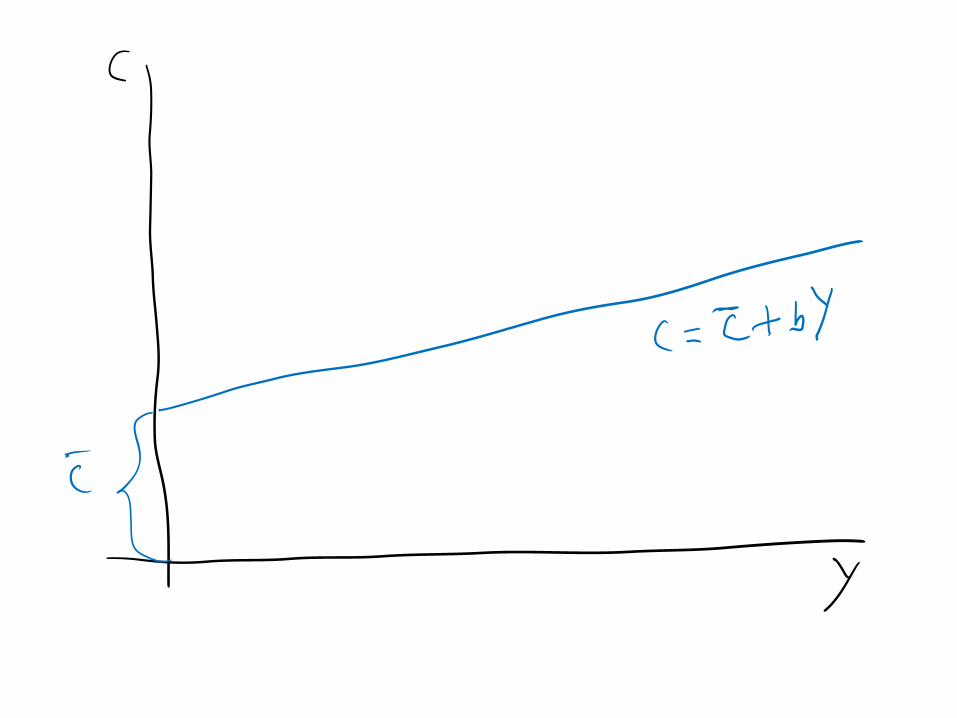
Key Drivers of Consumption

• Movements along the curve:

Current Disposable Income

• Shifts of the curve:

Changes in MPC (slope):

• Expected Future Disposable Income

• Wealth

• Interest Rates

– Changes in autonomous expenditures (intercept):

• Consumers’ State of Confidence

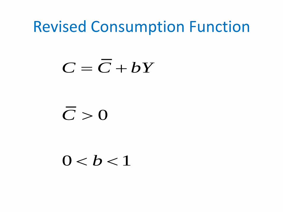
Revised Consumption Function

0

0 1

C C bY

C

b

= +

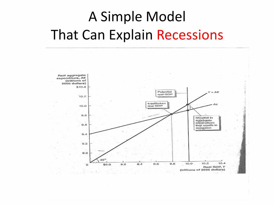
A Simple ModelThat Can Explain Recessions

A model: A grand but USEFUL simplification

• We strip away many important issues.

• We find a streamlined picture of the world.

• Despite the picture’s simplicity, we learn important things about how the real economy works.

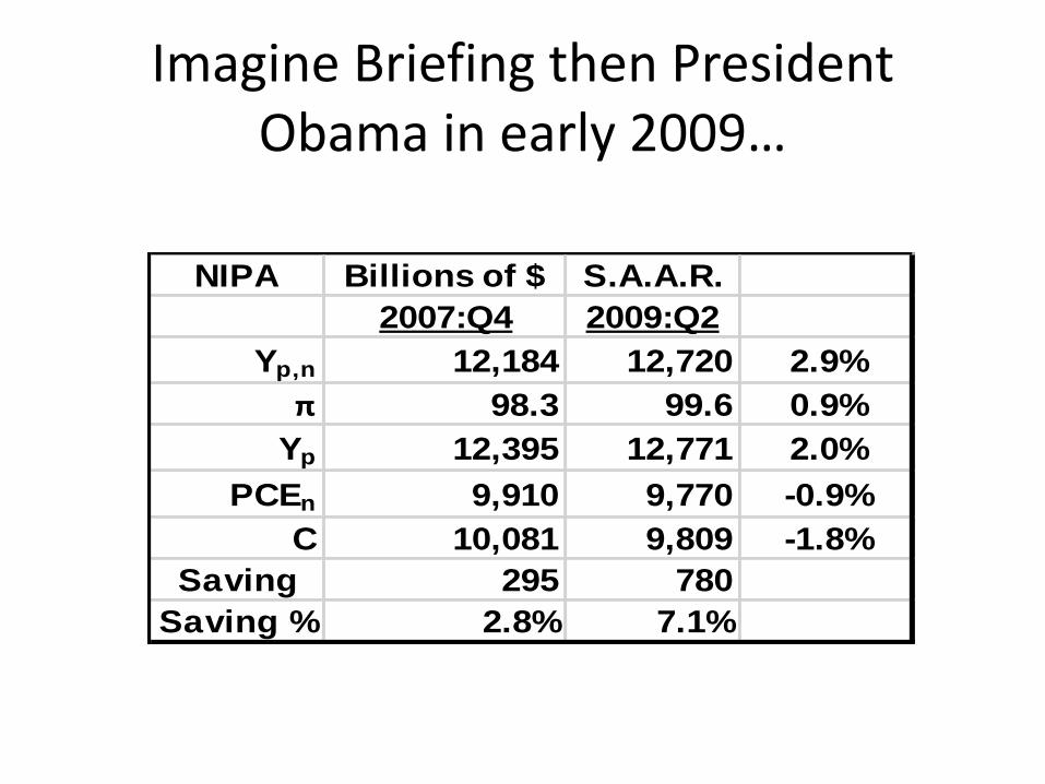
Imagine Briefing then President Obama in early 2009…

NIPA Billions of $ S.A.A.R.

2007:Q4 2009:Q2

Yp,n 12,184 12,720 2.9%

π 98.3 99.6 0.9%

Yp 12,395 12,771 2.0%

PCEn 9,910 9,770 -0.9%

C 10,081 9,809 -1.8%

Saving 295 780

Saving % 2.8% 7.1%

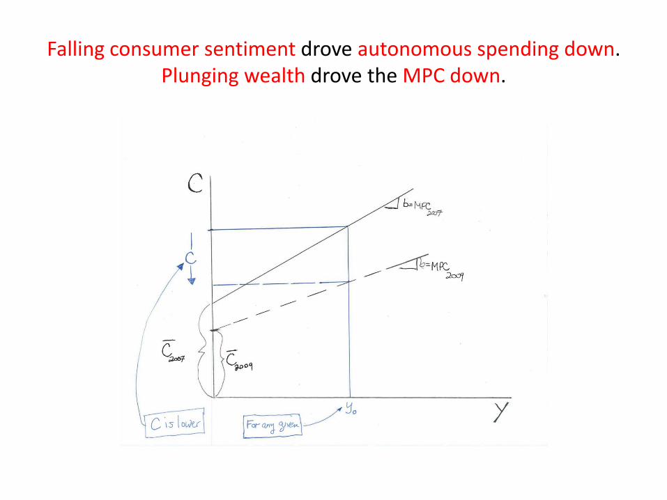
Falling consumer sentiment drove autonomous spending down.Plunging wealth drove the MPC down.

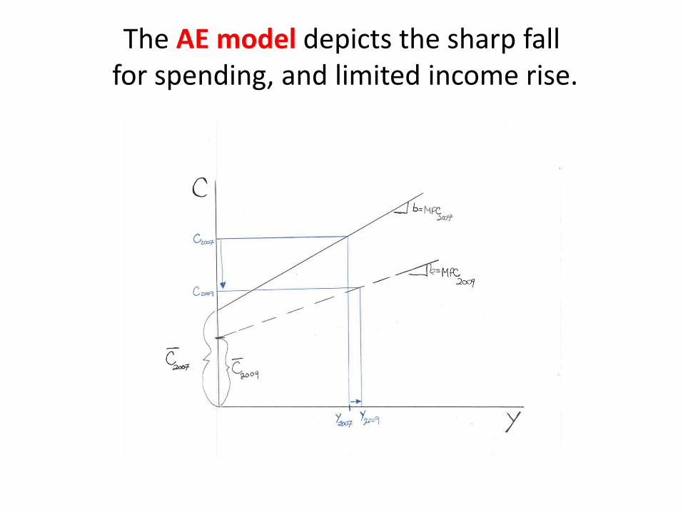
The AE model depicts the sharp fallfor spending, and limited income rise.

During 2011-2019, the flows into Inventory = 0.43% of Real GDP flows