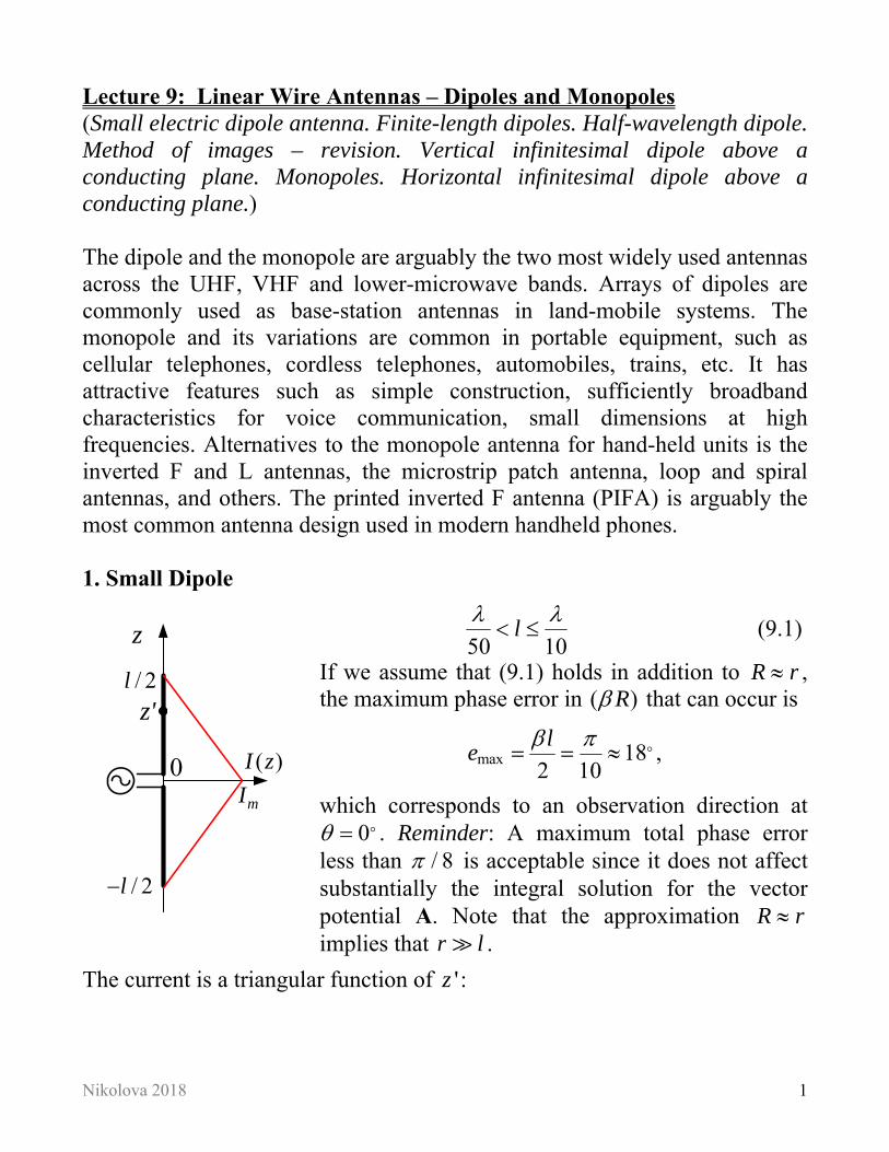
Nikolova 2018 1

Lecture 9: Linear Wire Antennas – Dipoles and Monopoles (Small electric dipole antenna. Finite-length dipoles. Half-wavelength dipole. Method of images – revision. Vertical infinitesimal dipole above a conducting plane. Monopoles. Horizontal infinitesimal dipole above a conducting plane.) The dipole and the monopole are arguably the two most widely used antennas across the UHF, VHF and lower-microwave bands. Arrays of dipoles are commonly used as base-station antennas in land-mobile systems. The monopole and its variations are common in portable equipment, such as cellular telephones, cordless telephones, automobiles, trains, etc. It has attractive features such as simple construction, sufficiently broadband characteristics for voice communication, small dimensions at high frequencies. Alternatives to the monopole antenna for hand-held units is the inverted F and L antennas, the microstrip patch antenna, loop and spiral antennas, and others. The printed inverted F antenna (PIFA) is arguably the most common antenna design used in modern handheld phones. 1. Small Dipole

50 10l

(9.1)

If we assume that (9.1) holds in addition to R r , the maximum phase error in ( )R that can occur is

max 182 10

le

,

which corresponds to an observation direction at 0 . Reminder: A maximum total phase error

less than / 8 is acceptable since it does not affect substantially the integral solution for the vector potential A. Note that the approximation R r implies that r l .

The current is a triangular function of 'z :

z

/ 2l

/ 2l

( )I z0

z'

mI

Nikolova 2018 2

'1 , 0 ' / 2

/ 2( ')

'1 , / 2 ' 0

/ 2

m

m

zI z l

lI z

zI l z

l

(9.2)

The VP integral is obtained as 0 /2

/2 0

' 'ˆ 1 ' 1 '

4 / 2 / 2

lj R j R

m m

l

z e z eI dz I dz

l R l R

A z . (9.3)

The solution of (9.3) is simple when we assume that R r :

1ˆ

2 4

j r

me

I lr

A z . (9.4)

The further away from the antenna the observation point is, the more accurate the expression in (9.4). Note that the result in (9.4) is exactly one-half of the result obtained for A of an infinitesimal dipole of the same length, if Im were the current uniformly distributed along the dipole. This is expected because we made the same approximation for R, as in the case of the infinitesimal dipole with a constant current distribution, and we integrated a triangular function along l, whose average is 0 0.5av mI I I .

Therefore, we need not repeat all the calculations of the field components, power and antenna parameters; we simply use the infinitesimal-dipole field multiplied by a factor of 0.5:

sin8

sin8

0

j rm

j rm

r r

I l eE j

rI l e

H jr

E E H H

, 1r . (9.5)

The normalized field pattern is the same as that of the infinitesimal dipole:

( , ) sinE . (9.6)

Nikolova 2018 3

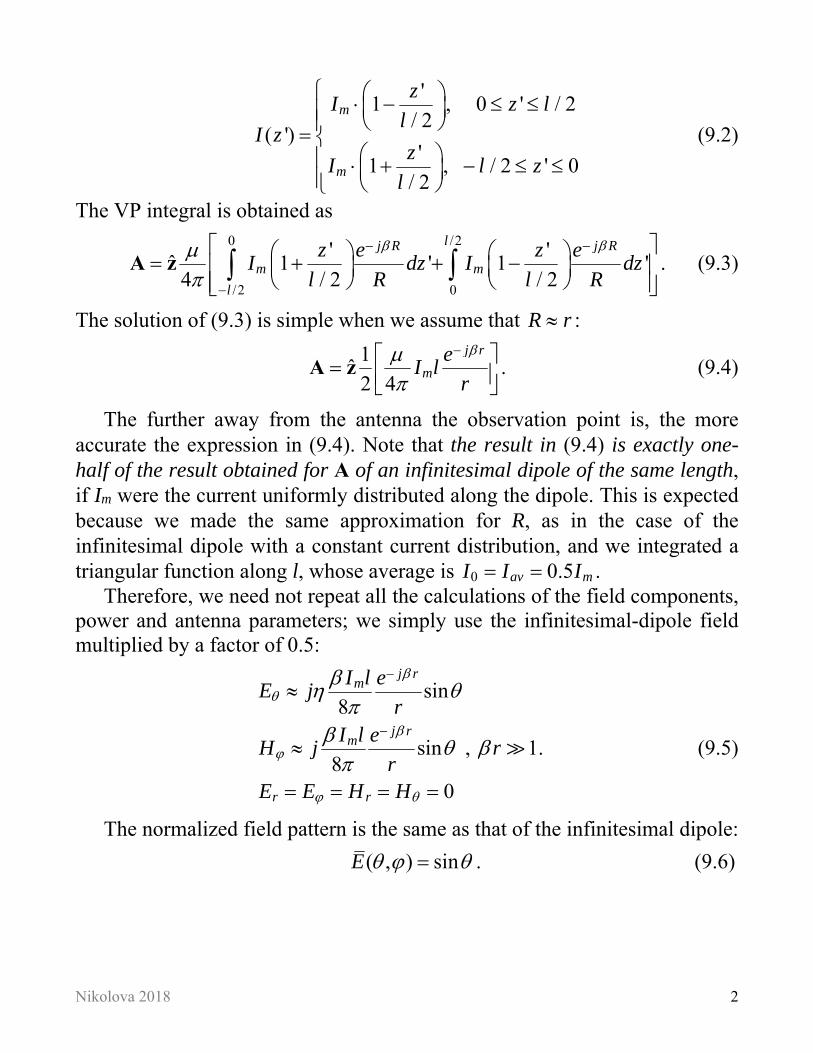
The power pattern: 2( , ) sinU (9.7)

-1

-0.5

0

0.5

1

-1 -0.5 0 0.5 1

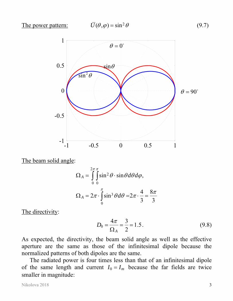
The beam solid angle: 2

2

0 0

3

0

sin sin ,

4 82 sin 2

3 3

A

A

d d

d

The directivity:

04 3

1.52A

D

. (9.8)

As expected, the directivity, the beam solid angle as well as the effective aperture are the same as those of the infinitesimal dipole because the normalized patterns of both dipoles are the same.

The radiated power is four times less than that of an infinitesimal dipole of the same length and current 0 mI I because the far fields are twice smaller in magnitude:

sin2sin

0

90

Nikolova 2018 4

2 21

4 3 12m mI l I l

. (9.9)

As a result, the radiation resistance is also four times smaller than that of the infinitesimal dipole:

2 2220

6r

l lR

. (9.10)

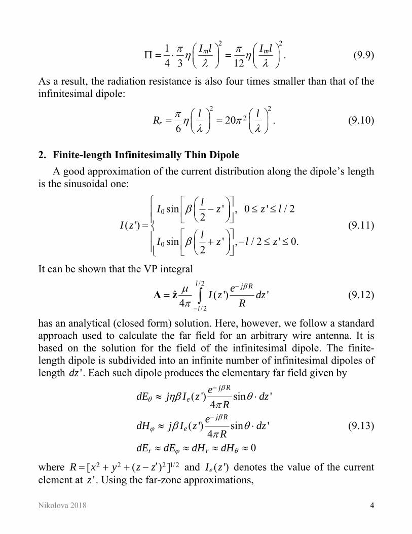
2. Finite-length Infinitesimally Thin Dipole

A good approximation of the current distribution along the dipole’s length is the sinusoidal one:

0

0

sin ' , 0 ' / 2 2

( ')

sin ' , / 2 ' 0.2

lI z z l

I zl

I z l z

(9.11)

It can be shown that the VP integral /2

/2

ˆ ( ') '4

l j R

l

eI z dz

R

A z (9.12)

has an analytical (closed form) solution. Here, however, we follow a standard approach used to calculate the far field for an arbitrary wire antenna. It is based on the solution for the field of the infinitesimal dipole. The finite-length dipole is subdivided into an infinite number of infinitesimal dipoles of length 'dz . Each such dipole produces the elementary far field given by

( ') sin '4

( ') sin '4

0

j R

e

j R

e

r r

edE j I z dz

Re

dH j I z dzR

dE dE dH dH

(9.13)

where 2 2 2 1/2[ ( ) ]R x y z z and ( ')eI z denotes the value of the current element at 'z . Using the far-zone approximations,

Nikolova 2018 5

1 1, for the amplitude factor

'cos , for the phase factorR rR r z

(9.14)

the following approximation of the elementary far field is obtained:

'cos sin '4

j rj z

ee

dE j I e dzr

. (9.15)

Using the superposition principle, the total far field is obtained as /2 /2

'cos

/2 /2

sin ( )4

l lj rj z

e

l l

eE dE j I z e dz

r

. (9.16)

The first factor

( ) sinj re

g jr

(9.17)

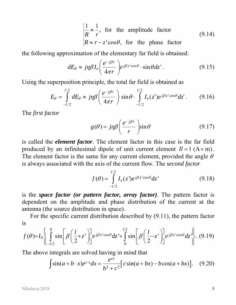
is called the element factor. The element factor in this case is the far field produced by an infinitesimal dipole of unit current element 1 (A m)Il . The element factor is the same for any current element, provided the angle is always associated with the axis of the current flow. The second factor

/2'cos

/2

( ) ( ') 'l

j ze

l

f I z e dz

(9.18)

is the space factor (or pattern factor, array factor). The pattern factor is dependent on the amplitude and phase distribution of the current at the antenna (the source distribution in space).

For the specific current distribution described by (9.11), the pattern factor is

0 /2'cos 'cos

0

/2 0

( ) sin ' ' sin ' '2 2

.l

j z j z

l

l lf I z e dz z e dz

(9.19)

The above integrals are solved having in mind that

2 2

sin( ) sin( ) cos( )cx

c x ea b x e dx c a bx b a bx

b c

. (9.20)

Nikolova 2018 6

The far field of the finite-length dipole is obtained as

0

cos cos cos2 2

( ) ( )2 sin

j r

l le

E g f j Ir

. (9.21)

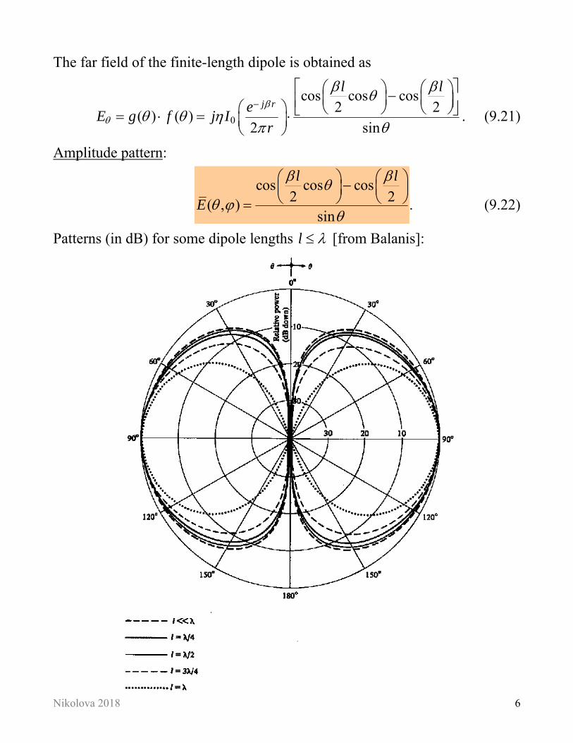
Amplitude pattern:

cos cos cos2 2( , )

sin

l l

E

. (9.22)

Patterns (in dB) for some dipole lengths l [from Balanis]:

Nikolova 2018 7

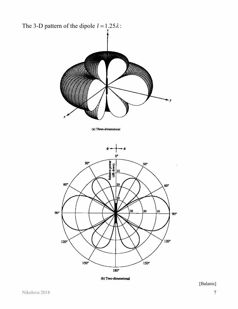
The 3-D pattern of the dipole 1.25l :

[Balanis]

Nikolova 2018 8

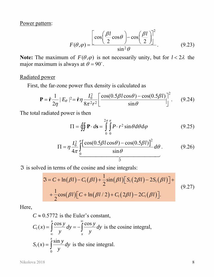
Power pattern: 2

2

cos cos cos2 2

( , )sin

l l

F

. (9.23)

Note: The maximum of ( , )F is not necessarily unity, but for 2l the major maximum is always at 90 . Radiated power

First, the far-zone power flux density is calculated as 22

022 2

1 cos(0.5 cos ) cos(0.5 )ˆ ˆ| |

2 8 sin

I l lE

r

P r r . (9.24)

The total radiated power is then 2

2

0 0

sind P r d d

P s (9.25)

220

0

cos(0.5 cos ) cos(0.5 )

4 sin

l lId

. (9.26)

is solved in terms of the cosine and sine integrals:

1ln sin 2 2

21

cos ln / 2 2 2 .2

i i i

i i

C l C l l S l S l

l C l C l C l

(9.27)

Here,

0.5772C is the Euler’s constant,

cos cos( )

x

i

x

y yC x dy dy

y y

is the cosine integral,

0

sin( )

x

iy

S x dyy

is the sine integral.

Nikolova 2018 9

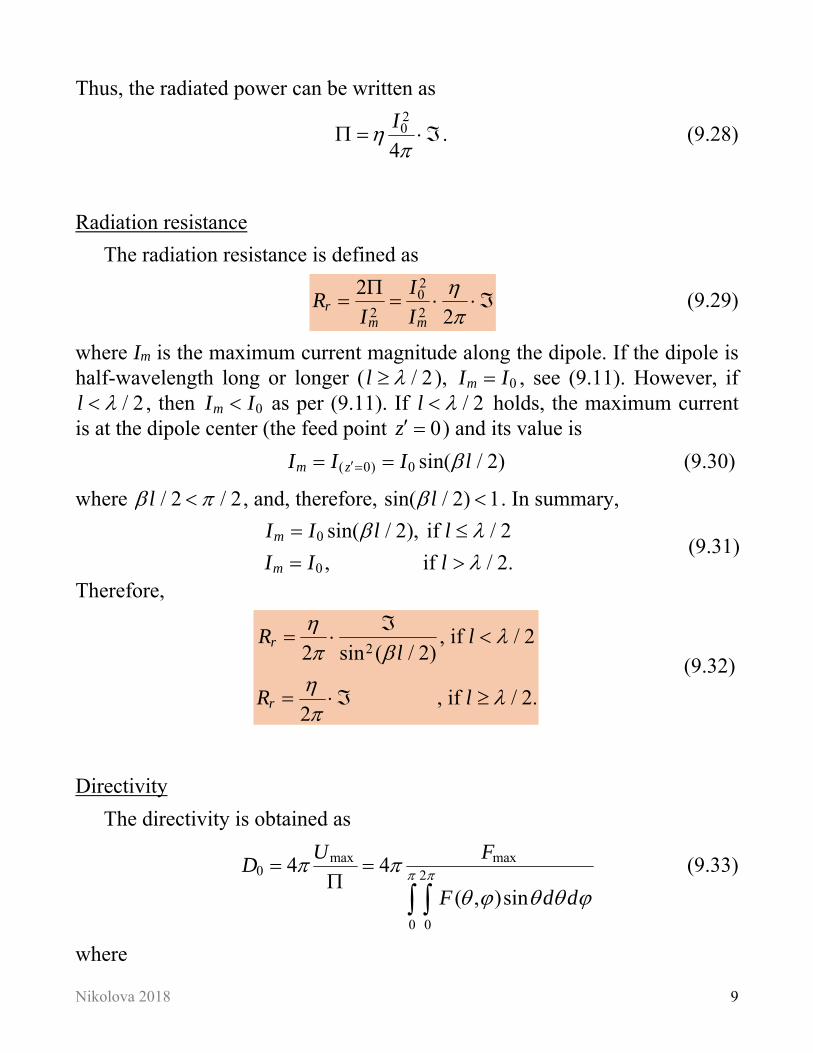
Thus, the radiated power can be written as 20

4

I

. (9.28)

Radiation resistance

The radiation resistance is defined as 20

2 2

2

2r

m m

IR

I I

(9.29)

where Im is the maximum current magnitude along the dipole. If the dipole is half-wavelength long or longer ( / 2l ), 0mI I , see (9.11). However, if

/ 2l , then 0mI I as per (9.11). If / 2l holds, the maximum current is at the dipole center (the feed point 0z ) and its value is

( 0) 0 sin( / 2)m zI I I l (9.30)

where / 2 / 2l , and, therefore, sin( / 2) 1l . In summary,

0

0

sin( / 2), if / 2

, if / 2.m

m

I I l l

I I l

(9.31)

Therefore,

2

, if / 22 sin ( / 2)

, if / 2.2

r

r

R ll

R l

(9.32)

Directivity

The directivity is obtained as

max max0 2

0 0

4 4

( , )sin

U FD

F d d

(9.33)

where

Nikolova 2018 10

2cos(0.5 cos ) cos(0.5 )

( , )sin

l lF

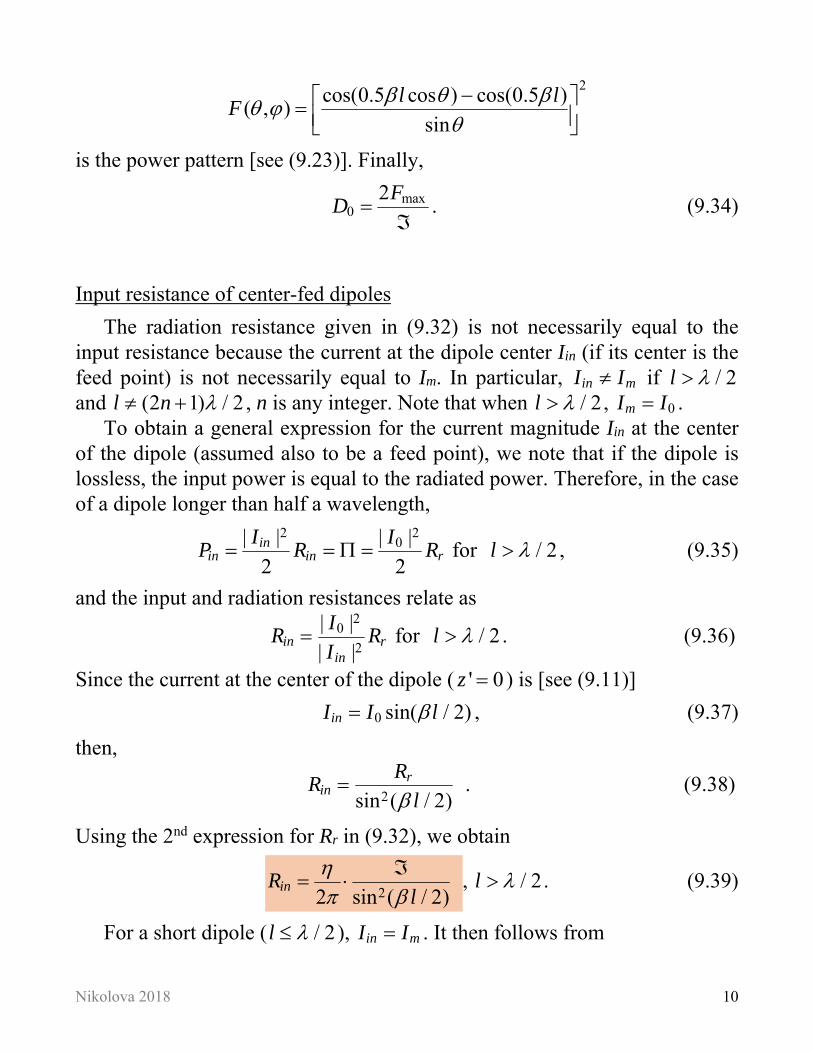
is the power pattern [see (9.23)]. Finally,

max0

2FD

. (9.34)

Input resistance of center-fed dipoles

The radiation resistance given in (9.32) is not necessarily equal to the input resistance because the current at the dipole center Iin (if its center is the feed point) is not necessarily equal to Im. In particular, in mI I if / 2l and (2 1) / 2l n , n is any integer. Note that when / 2l , 0mI I .

To obtain a general expression for the current magnitude Iin at the center of the dipole (assumed also to be a feed point), we note that if the dipole is lossless, the input power is equal to the radiated power. Therefore, in the case of a dipole longer than half a wavelength,

2 20| | | |

2 2in

in in rI I

P R R for / 2l , (9.35)

and the input and radiation resistances relate as

2

0

2

| || |

in rin

IR R

I for / 2l . (9.36)

Since the current at the center of the dipole ( ' 0z ) is [see (9.11)]

0 sin( / 2)inI I l , (9.37)

then,

2sin ( / 2)

rin

RR

l . (9.38)

Using the 2nd expression for Rr in (9.32), we obtain

22 sin ( / 2)inR

l

, / 2l . (9.39)

For a short dipole ( / 2l ), in mI I . It then follows from

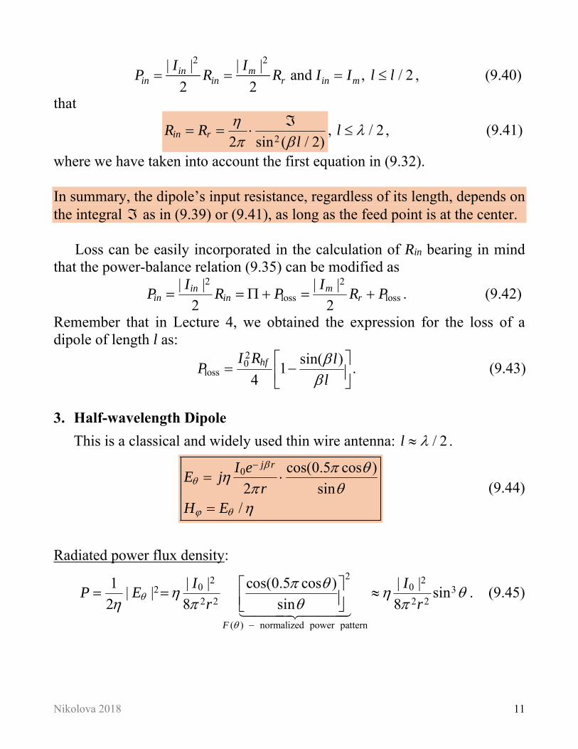
Nikolova 2018 11

2 2| | | |

and , / 22 2in m

in in r in mI I

P R R I I l l , (9.40)

that

22 sin ( / 2)

in rR Rl

, / 2l , (9.41)

where we have taken into account the first equation in (9.32). In summary, the dipole’s input resistance, regardless of its length, depends on the integral as in (9.39) or (9.41), as long as the feed point is at the center.

Loss can be easily incorporated in the calculation of Rin bearing in mind

that the power-balance relation (9.35) can be modified as

2 2

loss loss| | | |

2 2in m

in in rI I

P R P R P . (9.42)

Remember that in Lecture 4, we obtained the expression for the loss of a dipole of length l as:

20

losssin( )

14

hfI R lP

l

. (9.43)

3. Half-wavelength Dipole

This is a classical and widely used thin wire antenna: / 2l .

0 cos(0.5 cos )

2 sin/

j rI eE j

rH E

(9.44)

Radiated power flux density:

22 20 02 32 2 2 2

( ) normalized power pattern

1 | | cos(0.5 cos ) | || | sin

2 8 sin 8F

I IP E

r r

. (9.45)

Nikolova 2018 12

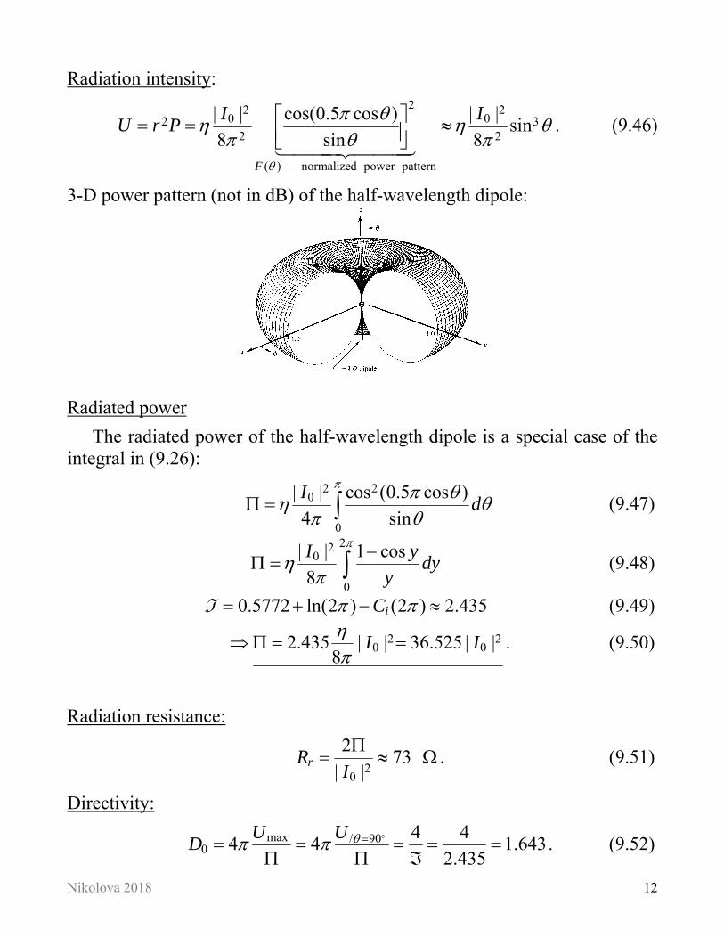
Radiation intensity: 22 2

0 02 32 2

( ) normalized power pattern

| | cos(0.5 cos ) | |sin

8 sin 8F

I IU r P

. (9.46)

3-D power pattern (not in dB) of the half-wavelength dipole:

Radiated power

The radiated power of the half-wavelength dipole is a special case of the integral in (9.26):

2 2

0

0

| | cos (0.5 cos )

4 sin

Id

(9.47)

22

0

0

| | 1 cos

8

I ydy

y

(9.48)

0.5772 ln(2 ) (2 ) 2.435iC I (9.49)

2 20 02.435 | | 36.525 | |

8I I

. (9.50)

Radiation resistance:

2

0

273

| |rR

I

. (9.51)

Directivity:

max / 900

4 44 4 1.643

2.435

U UD

. (9.52)

Nikolova 2018 13

Maximum effective area:

2

20 0.13

4eA D

. (9.53)

Input impedance

Since / 2l , the input resistance is

73in rR R . (9.54)

The imaginary part of the input impedance is approximately 42.5j . To acquire maximum power transfer, this reactance has to be removed by matching (e.g., shortening) the dipole:

thick dipole 0.47l thin dipole 0.48l .

The input reactance of the dipole is very frequency sensitive; i.e., it depends strongly on the ratio /l . This is to be expected from a resonant narrow-band structure operating at or near resonance such as the half-wavelength dipole. We should also keep in mind that the input impedance is influenced by the capacitance associated with the physical junction to the transmission line. The structure used to support the antenna, if any, can also influence the input impedance. That is why the curves below describing the antenna impedance are only representative.

Nikolova 2018 14

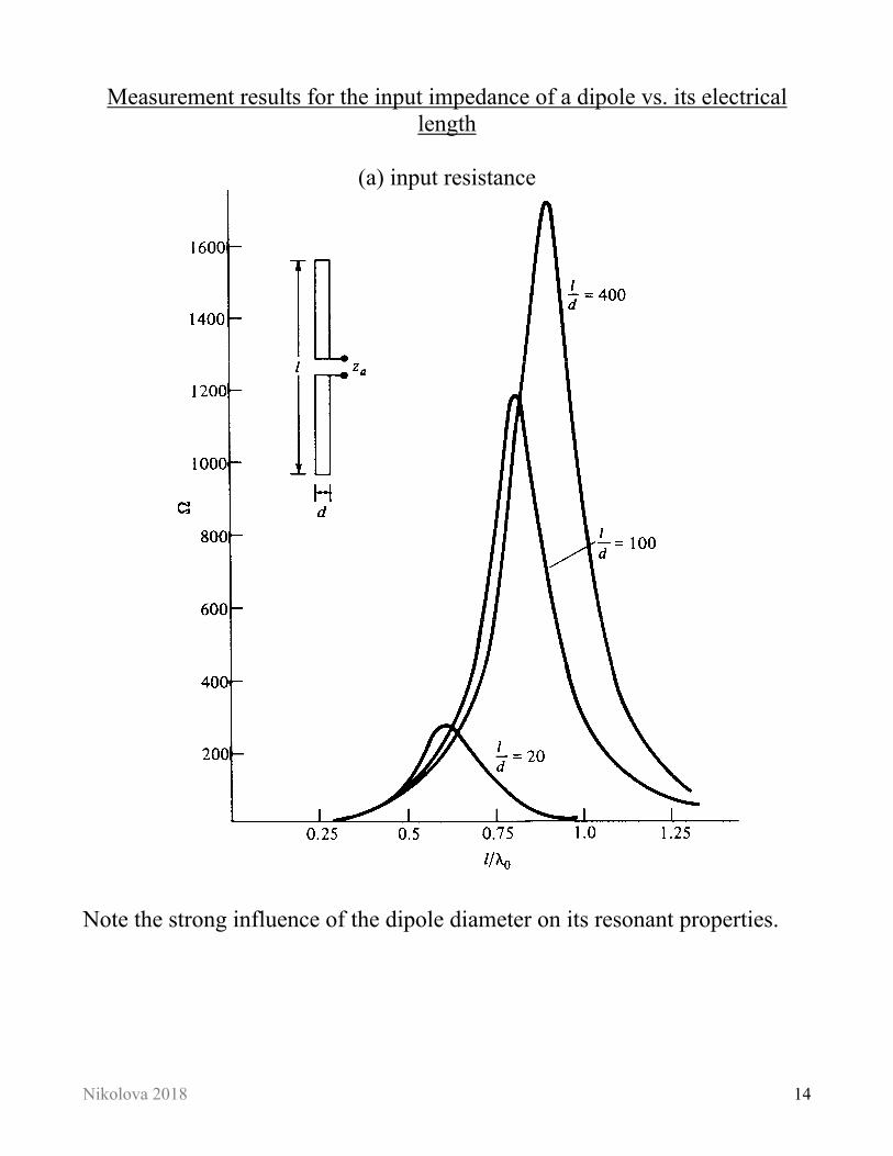
Measurement results for the input impedance of a dipole vs. its electrical length

(a) input resistance

Note the strong influence of the dipole diameter on its resonant properties.

Nikolova 2018 15

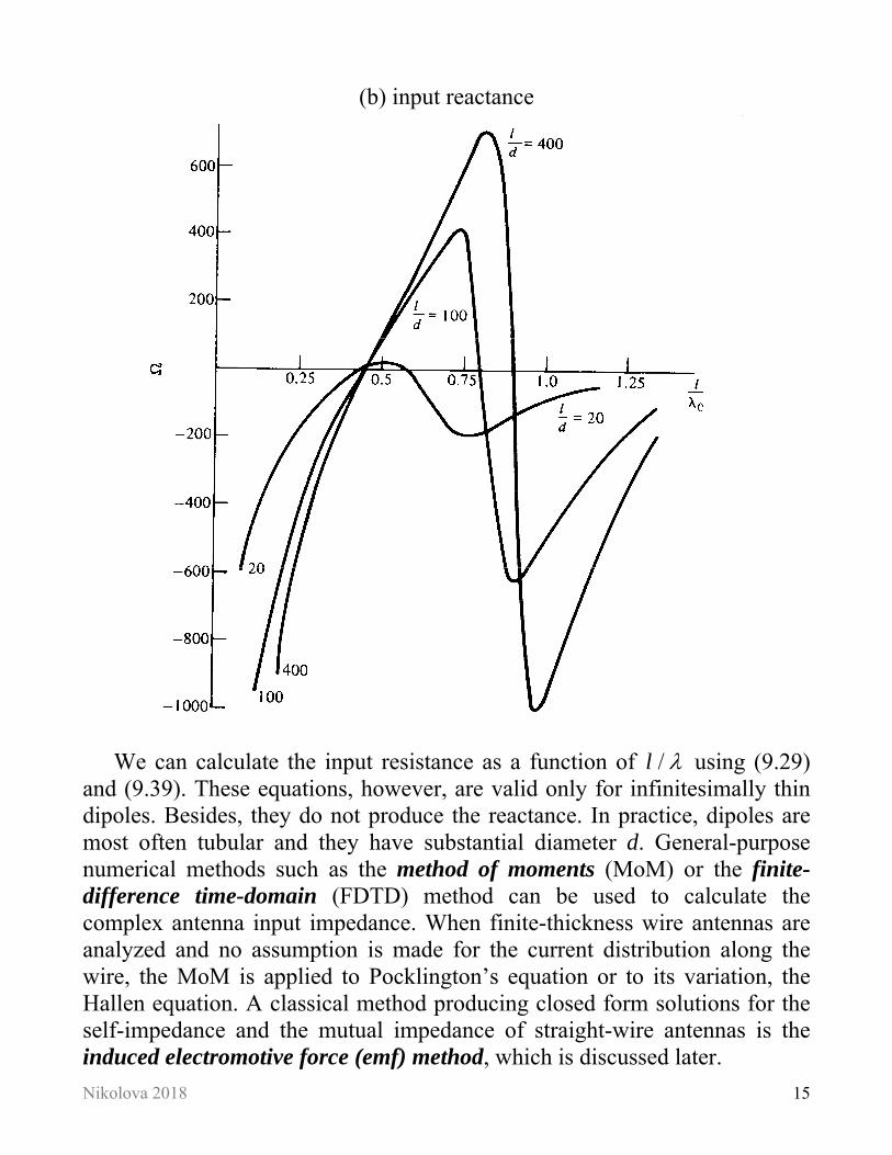
(b) input reactance

We can calculate the input resistance as a function of /l using (9.29) and (9.39). These equations, however, are valid only for infinitesimally thin dipoles. Besides, they do not produce the reactance. In practice, dipoles are most often tubular and they have substantial diameter d. General-purpose numerical methods such as the method of moments (MoM) or the finite-difference time-domain (FDTD) method can be used to calculate the complex antenna input impedance. When finite-thickness wire antennas are analyzed and no assumption is made for the current distribution along the wire, the MoM is applied to Pocklington’s equation or to its variation, the Hallen equation. A classical method producing closed form solutions for the self-impedance and the mutual impedance of straight-wire antennas is the induced electromotive force (emf) method, which is discussed later.

Nikolova 2018 16

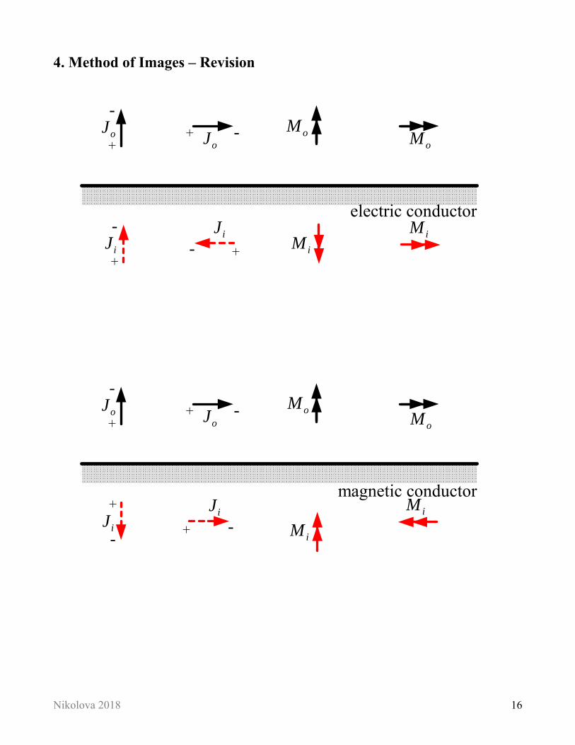
4. Method of Images – Revision

magnetic conductor+

-iJ

+

-oJ + -

oJ oMoM

+ -iJ

iMiM

electric conductor

oM

+

-iJ

+

-oJ

+-iJ

+ -oJ oM

iMiM

Nikolova 2018 17

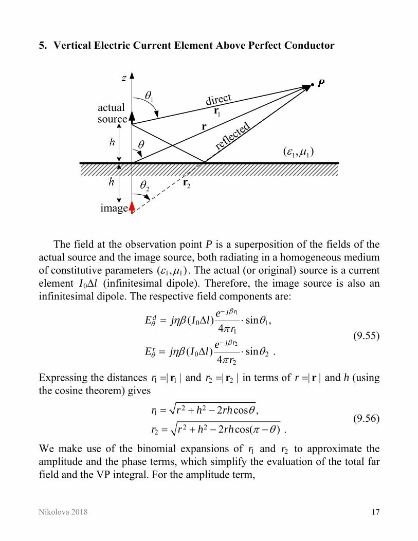
5. Vertical Electric Current Element Above Perfect Conductor

1

2

1r

2r

1 1( , )

r

direct

reflec

ted

image

actualsource

The field at the observation point P is a superposition of the fields of the actual source and the image source, both radiating in a homogeneous medium of constitutive parameters 1 1( , ) . The actual (or original) source is a current element 0I l (infinitesimal dipole). Therefore, the image source is also an infinitesimal dipole. The respective field components are:

1

2

0 11

0 22

( ) sin ,4

( ) sin .4

j rd

j rr

eE j I l

r

eE j I l

r

(9.55)

Expressing the distances 1 1| |r r and 2 2| |r r in terms of | |r r and h (using the cosine theorem) gives

2 21

2 22

2 cos ,

2 cos( ) .

r r h rh

r r h rh

(9.56)

We make use of the binomial expansions of 1r and 2r to approximate the amplitude and the phase terms, which simplify the evaluation of the total far field and the VP integral. For the amplitude term,

Nikolova 2018 18

1 2

1 1 1r r r . (9.57)

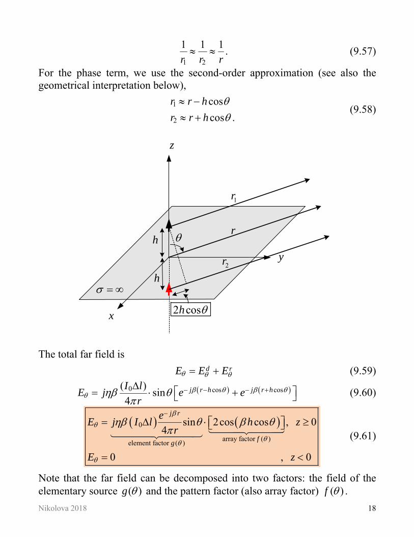
For the phase term, we use the second-order approximation (see also the geometrical interpretation below),

1

2

cos

cos .

r r h

r r h

(9.58)

x

y

z

h

h

2 cosh

1r

2r

r

The total far field is d rE E E (9.59)

0 cos cos( )sin

4j r h j r hI l

E j e er

(9.60)

0

array factor ( )element factor ( )

sin 2cos cos , 04

0 , 0

j r

fg

eE j I l h z

r

E z

(9.61)

Note that the far field can be decomposed into two factors: the field of the elementary source ( )g and the pattern factor (also array factor) ( )f .

Nikolova 2018 19

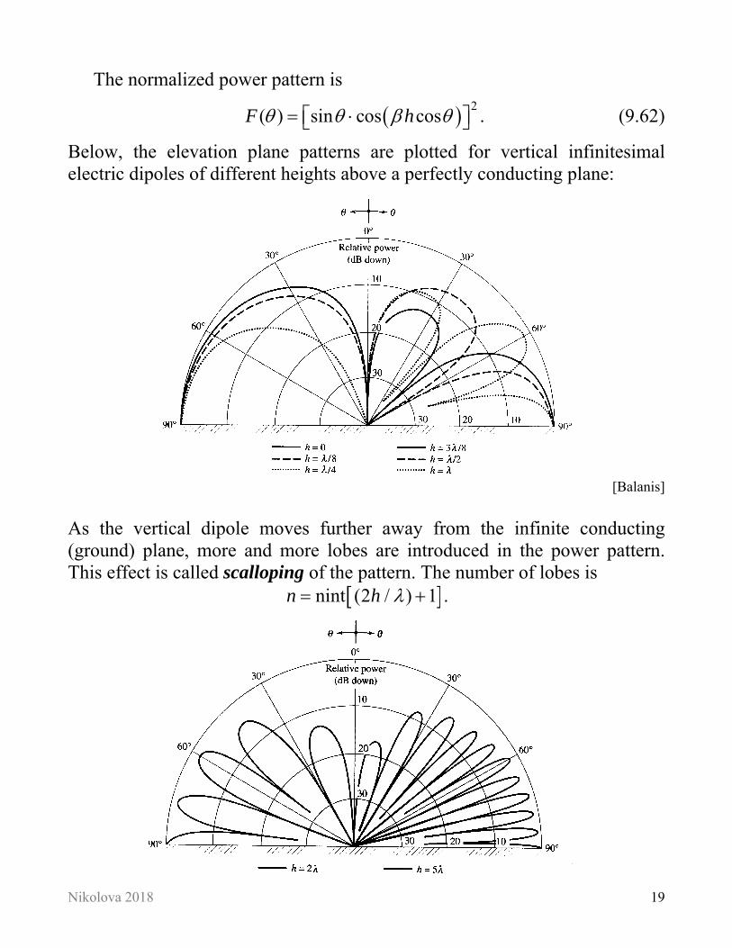
The normalized power pattern is

2( ) sin cos cosF h . (9.62)

Below, the elevation plane patterns are plotted for vertical infinitesimal electric dipoles of different heights above a perfectly conducting plane:

[Balanis]

As the vertical dipole moves further away from the infinite conducting (ground) plane, more and more lobes are introduced in the power pattern. This effect is called scalloping of the pattern. The number of lobes is

nint (2 / ) 1n h .

Nikolova 2018 20

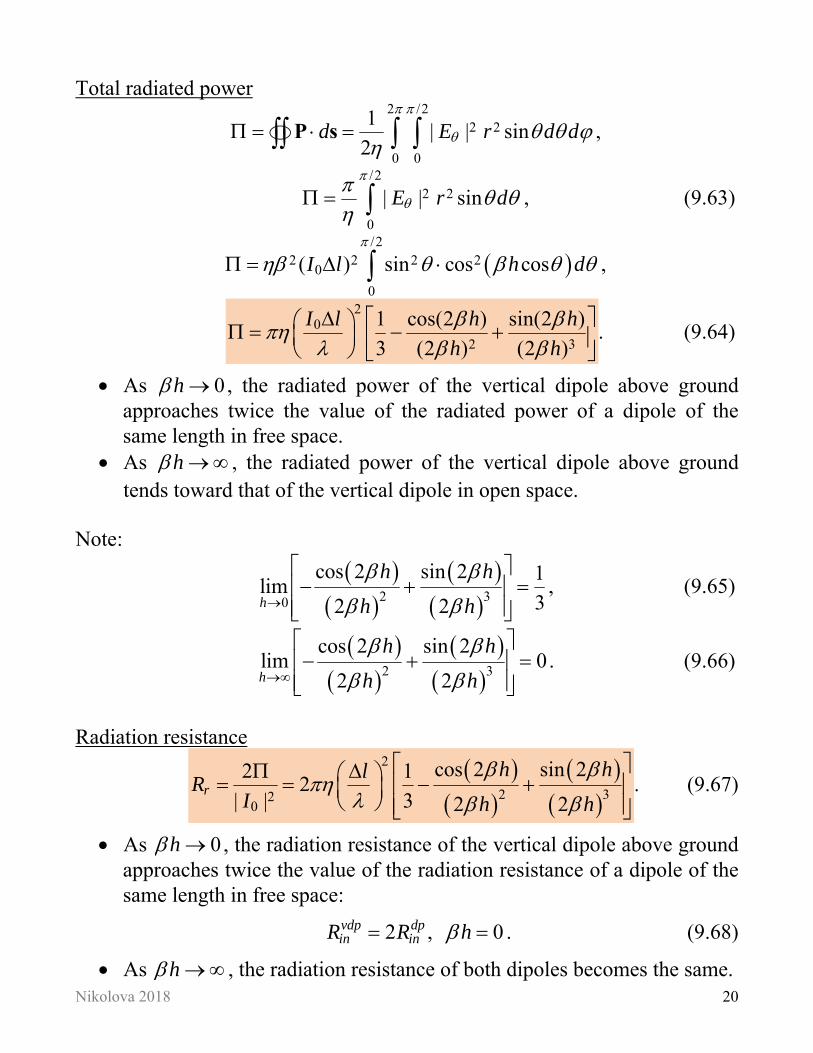
Total radiated power

2 /2

2 2

0 0

1| | sin

2d E r d d

P s ,

/2

2 2

0

| | sinE r d

, (9.63)

/2

2 2 2 20

0

( ) sin cos cosI l h d

,

2

0

2 3

1 cos(2 ) sin(2 )

3 (2 ) (2 )

I l h h

h h

. (9.64)

As 0h , the radiated power of the vertical dipole above ground approaches twice the value of the radiated power of a dipole of the same length in free space.

As h , the radiated power of the vertical dipole above ground tends toward that of the vertical dipole in open space.

Note:

2 30

cos 2 sin 2 1lim

32 2h

h h

h h

, (9.65)

2 3

cos 2 sin 2lim 0

2 2h

h h

h h

. (9.66)

Radiation resistance

2

2 320

cos 2 sin 22 12

| | 3 2 2r

h hlR

I h h

. (9.67)

As 0h , the radiation resistance of the vertical dipole above ground approaches twice the value of the radiation resistance of a dipole of the same length in free space:

2 , 0vdp dpin inR R h . (9.68)

As h , the radiation resistance of both dipoles becomes the same.

Nikolova 2018 21

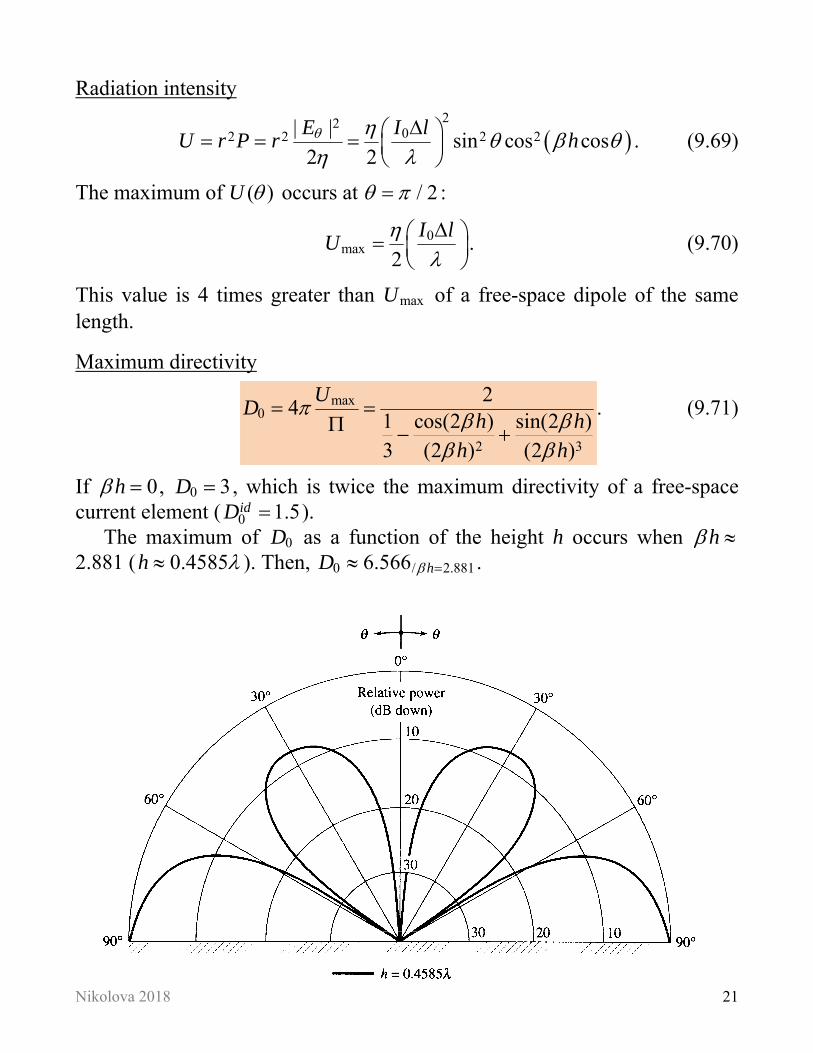
Radiation intensity

22

02 2 2 2| |sin cos cos

2 2

E I lU r P r h

. (9.69)

The maximum of ( )U occurs at / 2 :

0max

2

I lU

. (9.70)

This value is 4 times greater than maxU of a free-space dipole of the same length.

Maximum directivity

max0

2 3

24

1 cos(2 ) sin(2 )3 (2 ) (2 )

UD

h hh h

. (9.71)

If 0h , 0 3D , which is twice the maximum directivity of a free-space current element ( 0 1.5idD ).

The maximum of 0D as a function of the height h occurs when h 2.881 ( 0.4585h ). Then, 0 / 2.8816.566 hD .

Nikolova 2018 22

6. Monopoles

A monopole is a dipole that has been reduced by one-half and is fed against a ground plane. It is normally / 4 long (a quarter-wavelength monopole), but it might by shorter if there are space restrictions. Then, the monopole is a small monopole the counterpart of which is the small dipole (see Section 1). Its current has linear distribution with its maximum at the feed point and its null at the end.

The vertical monopole is a common antenna for AM broadcasting (f = 500 to 1500 kHz, = 200 to 600 m), because it is the shortest most efficient antenna at these frequencies as well as because vertically polarized waves suffer less attenuation at close-to-ground propagation. Vertical monopoles are widely used as base-station antennas in mobile communications, too.

Monopoles at base stations and radio-broadcast stations are supported by towers and guy wires. The guy wires must be separated into short enough ( / 8 ) pieces insulated from each other to suppress parasitic currents.

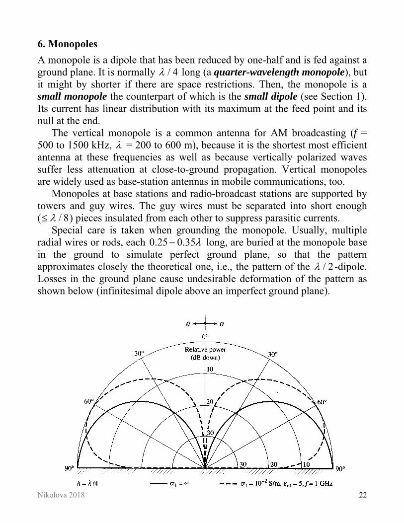
Special care is taken when grounding the monopole. Usually, multiple radial wires or rods, each 0.25 0.35 long, are buried at the monopole base in the ground to simulate perfect ground plane, so that the pattern approximates closely the theoretical one, i.e., the pattern of the / 2 -dipole. Losses in the ground plane cause undesirable deformation of the pattern as shown below (infinitesimal dipole above an imperfect ground plane).

Nikolova 2018 23

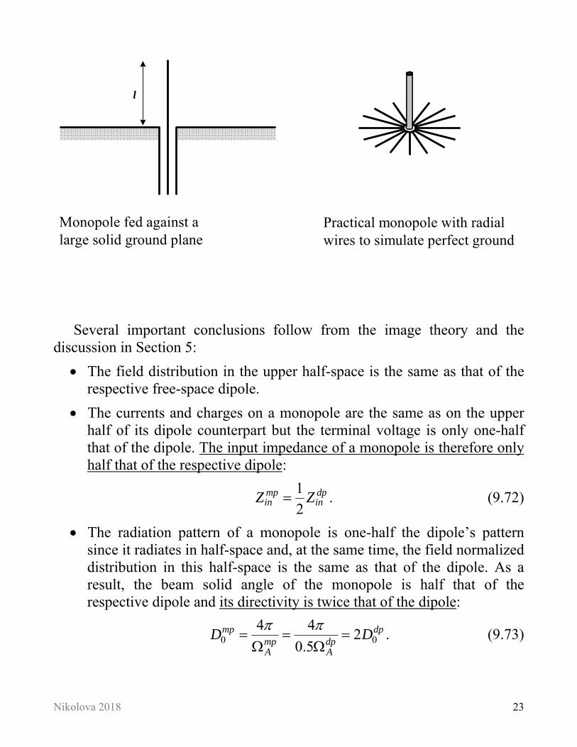
Monopole fed against alarge solid ground plane

Practical monopole with radialwires to simulate perfect ground

l

Several important conclusions follow from the image theory and the discussion in Section 5:

The field distribution in the upper half-space is the same as that of the respective free-space dipole.

The currents and charges on a monopole are the same as on the upper half of its dipole counterpart but the terminal voltage is only one-half that of the dipole. The input impedance of a monopole is therefore only half that of the respective dipole:

1

2mp dpin inZ Z . (9.72)

The radiation pattern of a monopole is one-half the dipole’s pattern since it radiates in half-space and, at the same time, the field normalized distribution in this half-space is the same as that of the dipole. As a result, the beam solid angle of the monopole is half that of the respective dipole and its directivity is twice that of the dipole:

0 04 4

20.5

mp dpmp dpA A

D D

. (9.73)

Nikolova 2018 24

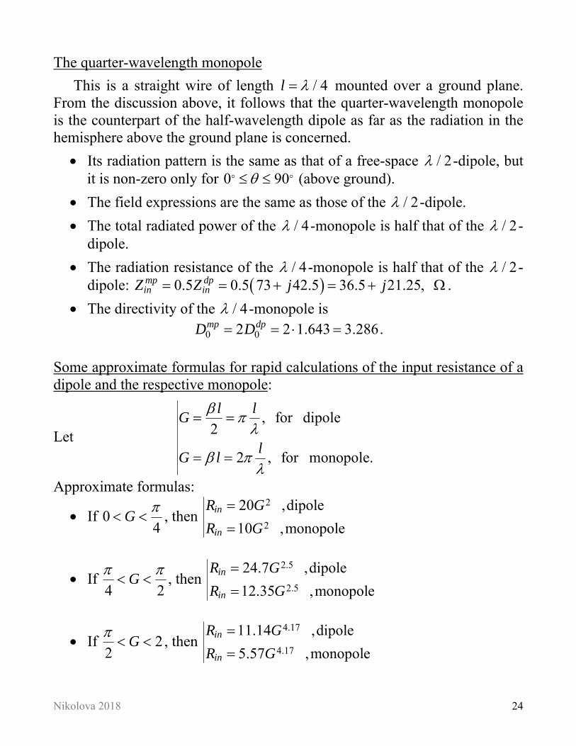
The quarter-wavelength monopole

This is a straight wire of length / 4l mounted over a ground plane. From the discussion above, it follows that the quarter-wavelength monopole is the counterpart of the half-wavelength dipole as far as the radiation in the hemisphere above the ground plane is concerned.

Its radiation pattern is the same as that of a free-space / 2 -dipole, but it is non-zero only for 0 90 (above ground).

The field expressions are the same as those of the / 2 -dipole.

The total radiated power of the / 4 -monopole is half that of the / 2 -dipole.

The radiation resistance of the / 4 -monopole is half that of the / 2 -dipole: 0.5 0.5 73 42.5 36.5 21.25,mp dp

in inZ Z j j .

The directivity of the / 4 -monopole is

0 02 2 1.643 3.286mp dpD D . Some approximate formulas for rapid calculations of the input resistance of a dipole and the respective monopole:

Let , for dipole

2

2 , for monopole.

l lG

lG l

Approximate formulas:

If 04

G

, then 2

2

20 ,dipole

10 ,monopolein

in

R G

R G

If 4 2

G , then

2.5

2.5

24.7 ,dipole

12.35 ,monopolein

in

R G

R G

If 22

G , then

4.17

4.17

11.14 ,dipole

5.57 ,monopolein

in

R G

R G

Nikolova 2018 25

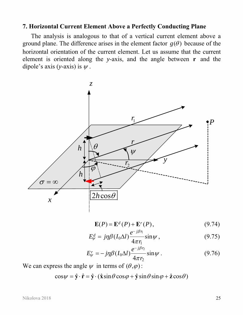
7. Horizontal Current Element Above a Perfectly Conducting Plane

The analysis is analogous to that of a vertical current element above a ground plane. The difference arises in the element factor ( )g because of the horizontal orientation of the current element. Let us assume that the current element is oriented along the y-axis, and the angle between r and the dipole’s axis (y-axis) is .

x

y

z

h

h

2 cosh

1r

2r

r

P

( ) ( ) ( )d rP P P E E E , (9.74)

1

01

( ) sin4

j rd e

E j I lr

, (9.75)

2

02

( ) sin4

j rr e

E j I lr

. (9.76)

We can express the angle in terms of ( , ) :

ˆˆ ˆ ˆ ˆ ˆcos ( sin cos sin sin cos ) y r y x y z

Nikolova 2018 26

2 2

cos sin sin

sin 1 sin sin .

(9.77)

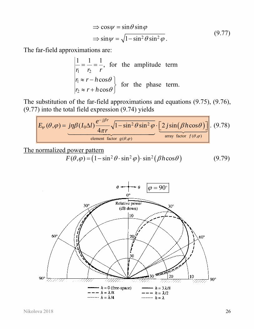
The far-field approximations are:

1 2

1

2

1 1 1, for the amplitude term

cosfor the phase term.

cos

r r r

r r h

r r h

The substitution of the far-field approximations and equations (9.75), (9.76), (9.77) into the total field expression (9.74) yields

2 20

array factor ( , )element factor ( , )

( , ) ( ) 1 sin sin 2 sin cos4

j r

fg

eE j I l j h

r

. (9.78)

The normalized power pattern 2 2 2( , ) 1 sin sin sin cosF h (9.79)

90

Nikolova 2018 27

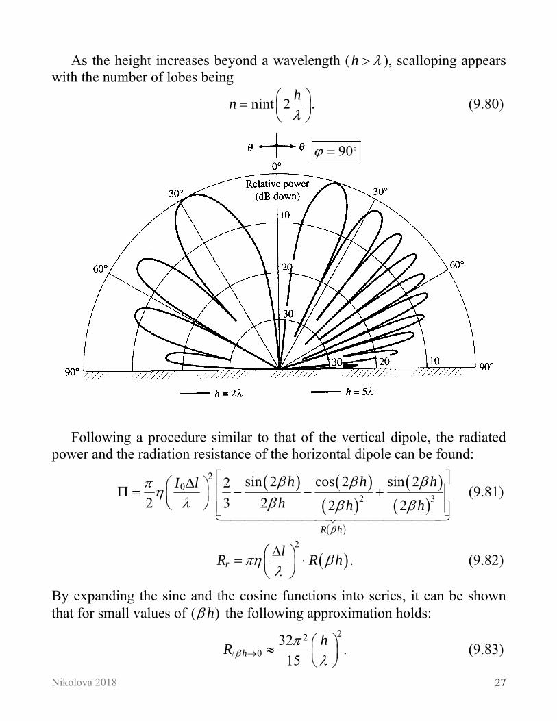
As the height increases beyond a wavelength (h ), scalloping appears with the number of lobes being

nint 2h

n

. (9.80)

Following a procedure similar to that of the vertical dipole, the radiated

power and the radiation resistance of the horizontal dipole can be found:

20

2 3

sin 2 cos 2 sin 22

2 3 2 2 2

R h

h h hI l

h h h

(9.81)

2

rl

R R h

. (9.82)

By expanding the sine and the cosine functions into series, it can be shown that for small values of ( )h the following approximation holds:

22

/ 032

15h

hR

. (9.83)

90

Nikolova 2018 28

It is also obvious that if 0h , then 0rR and 0 . This is to be expected because the dipole is short-circuited by the ground plane. Radiation intensity

22

02 2 2 2| | 1 sin sin sin cos2 2

r I lU h

E (9.84)

The maximum value of (9.84) depends on whether ( )h is less than / 2 or greater:

If 2

h

4h

2

0 2max / 0

sin2

I lU h

. (9.85)

If 2

h

4h

20

max/ arccos , 0

22

h

I lU

. (9.86)

Maximum directivity

If 4

h

, then maxU is obtained from (9.85) and the directivity is

2

max0

4sin ( )4

( )

U hD

R h

. (9.87)

If 4

h

, then maxU is obtained from (9.86) and the directivity is

max0

44

( )

UD

R h

. (9.88)

For very small h , the approximation 2

0sin

7.5h

Dh

is often used.