Lecture 5: Galaxy formation in CDM cosmologies

Inputs and assumptions:

• Gravitational instability, as in Lecture 4

• Dark matter and baryons are well-mixed,with F = Ωb/ΩDM ≈ 0.1 (“true” valuemore like F ≈ 0.2)

• Baryons dissipate (primarily through ra-diation)

• Angular momentum generate through tidaltorques (we’ll come back to this later)

• Dissipation is halted by angular momen-tum and/or star formation

• Spectrum of fluctuations coming from earlyUniverse (through, say, inflation)

1

Initial density fluctuation spectrum

We’ll represent the spectrum of initial fluctu-

ations as a power spectrum in Fourier space

and assume that the fluctuations are a Gaus-

sian random process with random phase. Since

the fluctuations are Gaussian, we can write

the distribution of the amplitudes of the per-

turbations of a given mass M as

p(δ) =1√

2πσ2(M)exp

[− δ2

2σ2(M)

],

where σ2(M) = 〈δ2〉 = 〈(δρ/ρ)2〉 is the mean-

squared fluctuation.

The real space fluctuations are

δ(r) =δρ(r)

ρ,

and therefore the Fourier transform gives us

the Fourier modes of the spectrum,

δk(k) =∫ +∞−∞

δ(r)eik·rdr

where the wavelength λ = 2π/k.

2

Let’s assume that the spectrum is a power-

law in k:

|δ2k | ∝ kn, (1)

where n is the power-law index of the fluctua-

tion spectrum. We can then show (Peebles,

LSS) that the rms density fluctuation in a

sphere of radius r is

〈δ2(r)〉 ∝ r−(3+n).

(This just comes from integrating the fluctu-

ation spectrum over a top-hat window func-

tion.) Then the rms density fluctuation in a

sphere of mass M enclosed by radius r is

〈δ2(r)〉 ∝ M−(3+n)/3 (2)

This is another of seeing how the density

fluctuation spectrum varies with scale. Note

that if n = 0 then 〈δ2(r)〉 ∝ M−1, which is

what should be the case for a random distri-

bution of matter.

3

Press-Schechter Theory

We want to know the number density of lumps

that have collapsed into bound objects at any

given time. First, we need to know what

overdensity corresponds to bound objects. We

can use our formulae from the last lecture to

compute the mean overdensity of a collapsing

object at maximum expansion with respect

to a universe (with Ω = 1 and Λ = 0) of

the same age, which has 〈ρ(t)〉 = (6πGt2)−1

when Ω = 1:

δ =3

20(6πt/tmax)

2/3.

The collapse of shell to r = 0 occurs at

t ≈ 2tmax, so the overdensity at this point

is, using our scaling formulae from last lec-

ture,

δc = (2tmax/t)2/3δi =3

20(12π)2/3 = 1.686.

4

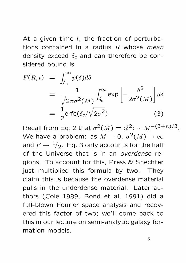
At a given time t, the fraction of perturba-

tions contained in a radius R whose mean

density exceed δc and can therefore be con-

sidered bound is

F (R, t) =∫ ∞δc

p(δ)dδ

=1√

2πσ2(M)

∫ ∞δc

exp

[− δ2

2σ2(M)

]dδ

=1

2erfc(δc/

√2σ2) (3)

Recall from Eq. 2 that σ2(M) = 〈δ2〉 ∼ M−(3+n)/3.

We have a problem: as M → 0, σ2(M) → ∞and F → 1/2. Eq. 3 only accounts for the half

of the Universe that is in an overdense re-

gions. To account for this, Press & Shechter

just multiplied this formula by two. They

claim this is because the overdense material

pulls in the underdense material. Later au-

thors (Cole 1989, Bond et al. 1991) did a

full-blown Fourier space analysis and recov-

ered this factor of two; we’ll come back to

this in our lecture on semi-analytic galaxy for-

mation models.5

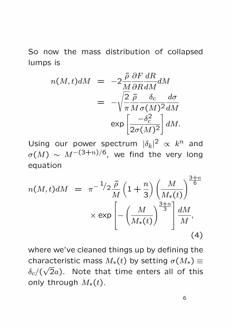
So now the mass distribution of collapsed

lumps is

n(M, t)dM = −2ρ

M

∂F

∂R

dR

dMdM

= −√

2

π

ρ

M

δc

σ(M)2dσ

dM

exp

[ −δ2c2σ(M)2

]dM.

Using our power spectrum |δk|2 ∝ kn and

σ(M) ∼ M−(3+n)/6, we find the very long

equation

n(M, t)dM = π−1/2

ρ

M

(1 +

n

3

) (M

M∗(t)

)3+n6

× exp

−

(M

M∗(t)

)3+n3

dM

M,

(4)

where we’ve cleaned things up by defining the

characteristic mass M∗(t) by setting σ(M∗) ≡δc/(

√2a). Note that time enters all of this

only through M∗(t).

6

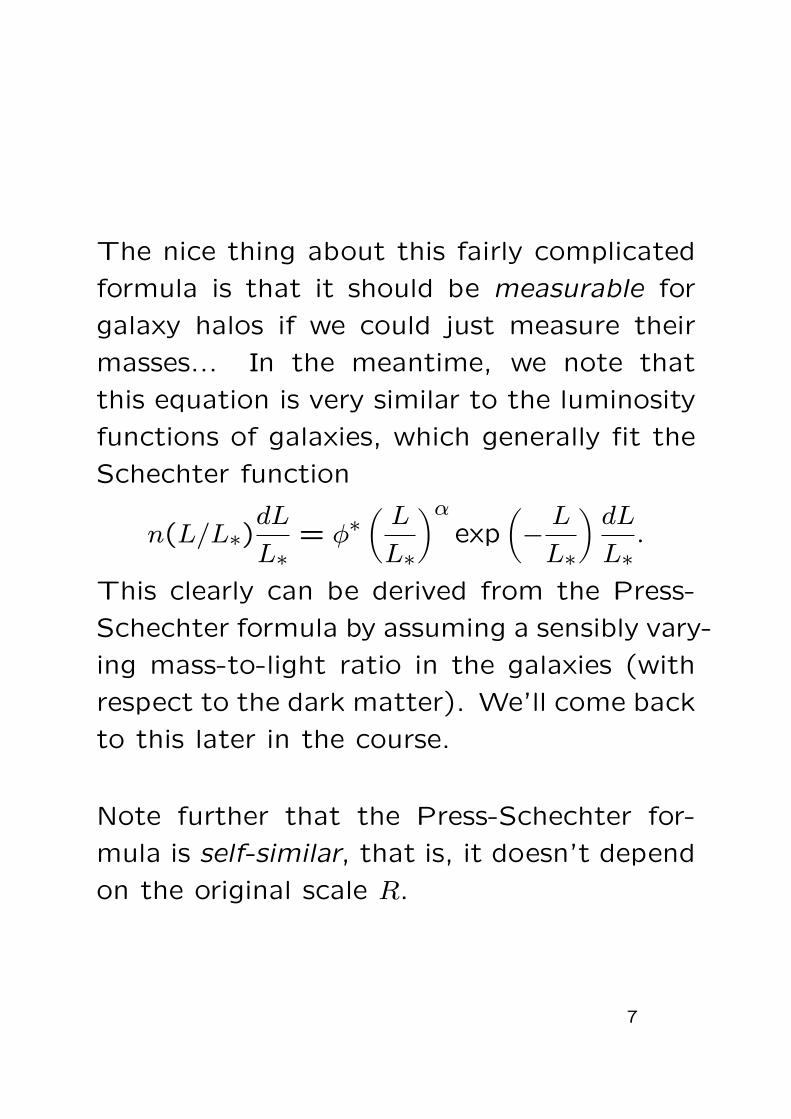
The nice thing about this fairly complicated

formula is that it should be measurable for

galaxy halos if we could just measure their

masses... In the meantime, we note that

this equation is very similar to the luminosity

functions of galaxies, which generally fit the

Schechter function

n(L/L∗)dL

L∗= φ∗

(L

L∗

)α

exp(− L

L∗

)dL

L∗.

This clearly can be derived from the Press-

Schechter formula by assuming a sensibly vary-

ing mass-to-light ratio in the galaxies (with

respect to the dark matter). We’ll come back

to this later in the course.

Note further that the Press-Schechter for-

mula is self-similar, that is, it doesn’t depend

on the original scale R.

7

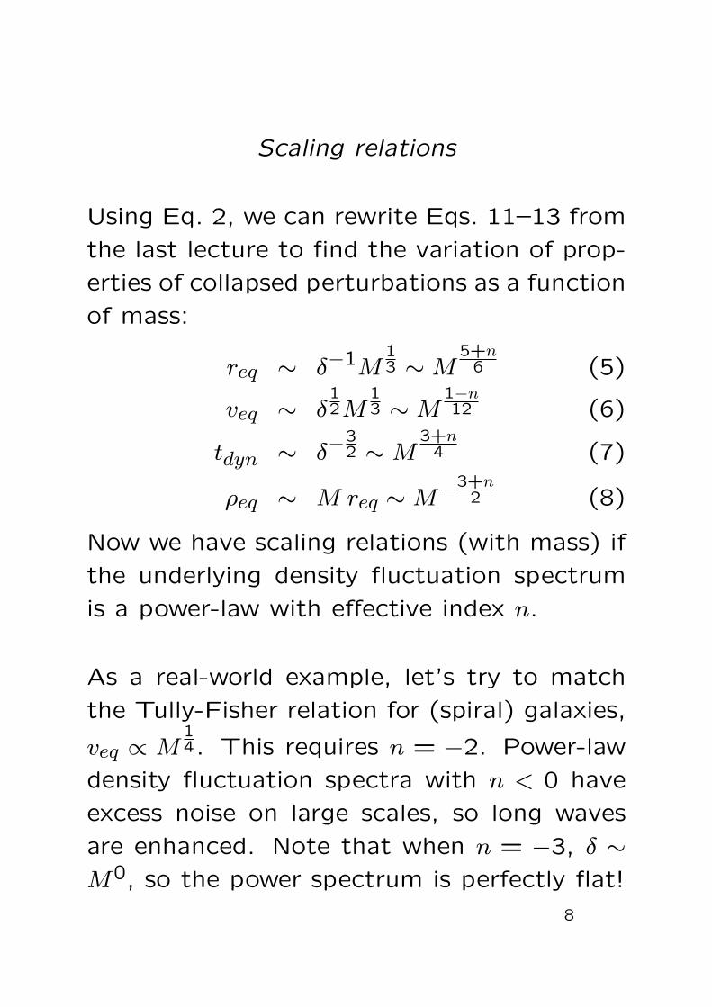
Scaling relations

Using Eq. 2, we can rewrite Eqs. 11–13 from

the last lecture to find the variation of prop-

erties of collapsed perturbations as a function

of mass:

req ∼ δ−1M13 ∼ M

5+n6 (5)

veq ∼ δ12M

13 ∼ M

1−n12 (6)

tdyn ∼ δ−32 ∼ M

3+n4 (7)

ρeq ∼ M req ∼ M−3+n2 (8)

Now we have scaling relations (with mass) if

the underlying density fluctuation spectrum

is a power-law with effective index n.

As a real-world example, let’s try to match

the Tully-Fisher relation for (spiral) galaxies,

veq ∝ M14. This requires n = −2. Power-law

density fluctuation spectra with n < 0 have

excess noise on large scales, so long waves

are enhanced. Note that when n = −3, δ ∼M0, so the power spectrum is perfectly flat!

8

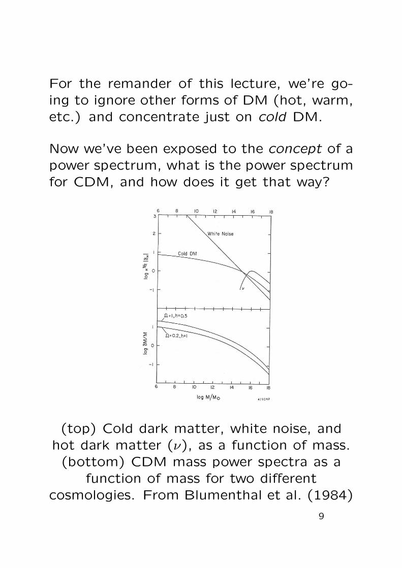
For the remander of this lecture, we’re go-ing to ignore other forms of DM (hot, warm,etc.) and concentrate just on cold DM.

Now we’ve been exposed to the concept of apower spectrum, what is the power spectrumfor CDM, and how does it get that way?

(top) Cold dark matter, white noise, andhot dark matter (ν), as a function of mass.(bottom) CDM mass power spectra as a

function of mass for two differentcosmologies. From Blumenthal et al. (1984)

9

At large masses—long wavelengths or small

k—the power spectrum is the initial power

spectrum (from, say, inflation), because these

masses are much bigger than the mass scale

when matter and radiation decouple (M ÀMdec ∼ 1016) and thus cross the horizon when

matter dominates. We typically choose n =

1 in this range (a Harrison–Peebles–Zel’dovich

spectrum), because we expect the Universe

to be homogeneous both at early times and

on the largest scales today. This also pre-

serves the constancy of fluctuation amplitude

with mass as the perturbations come through

the horizon. Note that we also typically as-

sume that

δDM = δb = δγ

initially, which represents the “adiabatic” mode

of the perturbations. There can be two other

modes, of course, but we generally ignore

them (ask Rien or Saleem).

10

At small masses (M ¿ Mdec), there is almost

no growth of fluctuations between the time

they cross the horizon with constant ampli-

tude and can’t grow because ρmatter < ργ.

They just accumulate and sit there with the

same amplitude until decoupling. (This can

be shown with about a page of algebra and a

nasty differential equation.) This is why the

CDM power spectrum is so flat at low masses

(M ∼< 1010 M¯). Moreover, radiation pres-

sure keeps baryon density fluctuations from

collapsing until after decouple because pho-

tons and baryons are locked together by elec-

tron scattering.

The most important lesson learned from

the CDM power spectrum is that δM/M de-

creases with increasing M , so small mass

fluctuations collapse first on average. Since

these small mass fluctuations are themselves

clustered within larger mass perturbations,

which collapse later, we have a hierarchy of

collapse in CDM cosmologies.

11

Can we compare our power spectra to real

systems in some way?

First, let’s define the “virial temperature” of

a gravitationally-bound system,

T =µv2

3k= 24.2 v2 K (9)

where µ is the mean molecular weight (roughly

10−24 g), k is Boltzmann’s constant, and v is

the three-dimensional virial velocity in km/s

(what we called veq in the last lecture). Then

for a total mass M , assuming M = 10Mb for

galaxies and M = Mvirial for groups and clus-

ters of galaxies, we find the following plot

using Eq. 5–8:

12

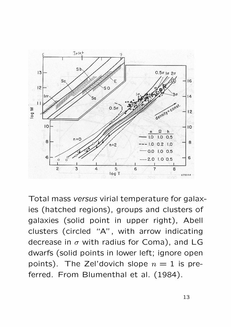
Total mass versus virial temperature for galax-

ies (hatched regions), groups and clusters of

galaxies (solid point in upper right), Abell

clusters (circled “A”, with arrow indicating

decrease in σ with radius for Coma), and LG

dwarfs (solid points in lower left; ignore open

points). The Zel’dovich slope n = 1 is pre-

ferred. From Blumenthal et al. (1984).

13

Different solid lines correspond to different

overdensities. Apparently, early-type galax-

ies come from 2–3σ fluctuations, spirals from

1–2σ fluctuations, and irregulars and most

dwarfs from ∼< 1σ peaks. Scaling relations

like Tully-Fisher (M ∼ v4 ∼ T2) evidently

arise from the slope of the density fluctua-

tion spectrum in the range of galaxy masses.

Note that the normalization of these curves is

actually set by the observed correlation func-

tion of galaxies, so agreement between the

predicted and observed amplitudes of the TF

and FJ relations is a major success of CDM.

14

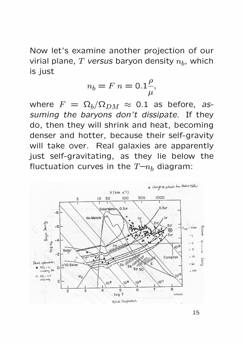
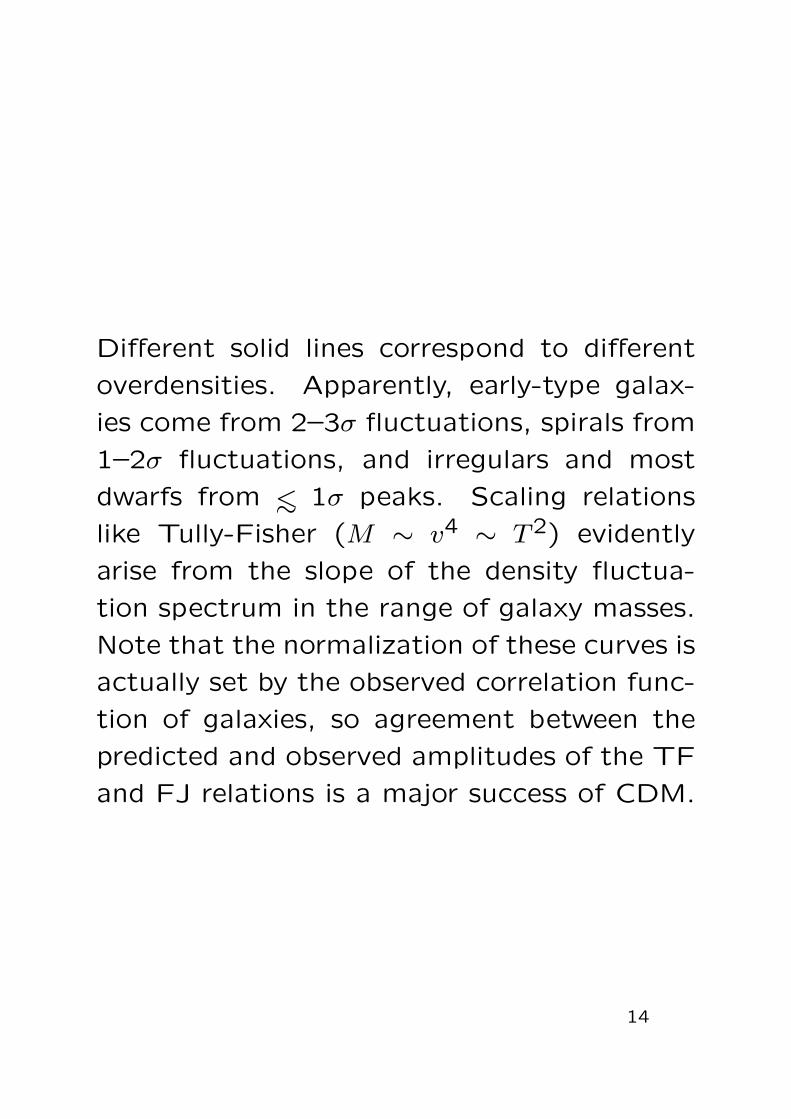
Now let’s examine another projection of ourvirial plane, T versus baryon density nb, whichis just

nb = F n = 0.1ρ

µ,

where F = Ωb/ΩDM ≈ 0.1 as before, as-suming the baryons don’t dissipate. If theydo, then they will shrink and heat, becomingdenser and hotter, because their self-gravitywill take over. Real galaxies are apparentlyjust self-gravitating, as they lie below thefluctuation curves in the T–nb diagram:

15

In this observed T–nb diagram (from Blumen-

thal et al. 1984), we see that groups and clus-

ters lie on the dissipationless curves, as ex-

pected (they’re dominated by dark matter),

but real galaxies, from dwarfs to irregulars to

spirals to ellipticals have suffered dissipation.

We expect cooling and therefore dissipation

when

tcool ∼< tdyn.

The cooling curves (which can be thought

of as the times at which tcool = tdyn) are

shown in the T–nb diagram for two differ-

ent metallicities. What physics are impor-

tant? When T < 104 K, H is neutral, and

cooling is dominated by permitted metal lines

(and maybe H2); when T ∼ 104–106, cool-

ing is very efficient through H recombination

and forbidden metal lines (e.g., H II regions);

when T > 106, cooling is dominated by ther-

mal bremsstrahlung in the X-ray plasma.

16

Note that the boundary between galaxies and

groups happens almost exactly at the cool-

ing curve boundary, and therefore this sim-

ple cooling model correctly predicts the exis-

tance of galaxies as opposed to larger struc-

tures as due to baryonic dissipation.

It is crucial to note here that the baryonic

densities are a factor of 1000 higher than the

virialization curves suggest, so the baryonic

component of galaxies fell in by about a fac-

tor of 10 in radius relative to the dark matter.

We will discuss the conservation and loss of

angular momentum during this collapse later

in the course.

17

Let’s quickly discuss biasing. In the bad old

days, when Ω0 = Ωm = 1, models of struc-

ture formation (like the “Gang of Four” mod-

els by Davis, Efstathiou, Frenk & White 1985)

tended to overproduce clustering of dark mat-

ter in the nonlinear region compared to galax-

ies. These authors and others—most no-

tably, Kaiser (1984), who invented the con-

cept of “biasing”—suggested that a “fudge

factor” b was required to match the models

to the observed density distribution. That is,

galaxies are a “biased” tracer of the underly-

ing mass distribution because the efficiency

of galaxy formation may depend in some non-

trivial way on that distribution.

18

Seen from another perspective, inflation mod-

els didn’t correctly predict the zeropoint of

the density fluctuation spectrum. Typically,

models are normalized so that(

δM

M

)

rms= 1

in a sphere of radius 800 km s−1 = 8h−1 Mpc.

In effect, this normalization assumes galaxies

trace matter on this scale. This normaliza-

tion can be adjusted using the bias parameter

b:(

δM

M

)DM

800 km s−1=

1

b

(δM

M

)gal

800 km s−1=

1

b

19

In CDM models, b is a free parameter. How-

ever, it has recently been measured by the

2dF Galaxy Redshift Survey (Verde et al.

2002) to have the value

b = 1.02± 0.11 (10)

on scales between 5 and 30h−1 Mpc, which

clearly means that optically-selected galaxies

are very good tracers of the mass in the lo-

cal Universe. It could be that other tracers

(like galaxies selected from IRAS in the near-

and mid-IR) are biased differently (Feldman

et al. 2001), but the data are generally con-

sistent these days with b = 1, and so biasing

is probably unimportant today and galaxies

can be used to trace the density fluctuation

spectrum. This is because we live in a low-

matter-density University and so clustering is

significantly reduced from the Ω0 = Ωm = 1

case.

20