Tension of the EG statistic and RSD data with Planck/ΛCDM and implications forweakening gravity.

F. Skara∗ and L. Perivolaropoulos†

Department of Physics, University of Ioannina, 45110 Ioannina, Greece(Dated: March 26, 2020)

The EG statistic is a powerful probe for detecting deviations from GR by combining weak lensing(WL), real-space clustering and redshift space distortion (RSD) measurements thus probing boththe lensing and the growth effective Newton constants (GL and Geff ). We construct an up todate compilation of EG statistic data including both redshift and scale dependence (EG(R, z)). Wecombine this EG data compilation with an up to date compilation of fσ8 data from RSD observationsto identify the current level of tension between the Planck/ΛCDM standard model based on generalrelativity and a general model independent redshift evolution parametrization of GL and Geff . Eachfσ8 datapoint considered has been published separately in the context of independent analyses ofdistinct galaxy samples. However, there are correlations among the datapoints considered due tooverlap of the analyzed galaxy samples. Due to these correlations the derived levels of tension ofthe best fit parameters with Planck/ΛCDM are somewhat overestimated but this is the price topay for maximizing the information encoded in the compilation considered. We find that the levelof tension increases from about 3.5σ for the fσ8 data compilation alone to about 6σ when the EG

data are also included in the analysis. The direction of the tension is the same as implied by thefσ8 RSD growth data alone (lower Ωm and/or weaker effective Newton constant at low redshifts forboth the lensing and the growth effective Newton constants (GL and Geff )). These results furtheramplify the hints for weakening modified gravity discussed in other recent analyses [1–4].

I. INTRODUCTION

The theory of general relativity (GR) and the standardΛ cold dark matter (ΛCDM) [5] cosmological model havebeen remarkably successful in explaining a wide array ofobservations [6] including the observed accelerating ex-pansion of the universe [7, 8]. Despite of its successesand simplicity, the validity of the cosmological standardmodel ΛCDM is currently under intense investigation.This is motivated by a range of profound theoretical andobservational difficulties of the model. The most impor-tant theoretical difficulties of the ΛCDM model are thefine tuning [9–11] and coincidence problems [12, 13]. Thefirst of these problems corresponds to the large discrep-ancy between observations and quantum field theoreticalpredictions on the value of the cosmological constant Λwhile the second is associated with the coincidence be-tween the observed vacuum energy density ΩΛ and thematter density Ωm which in the present epoch are of thesame order of magnitude despite of their very differentevolution during the cosmic history.

A well known observational difficulty corresponds tothe tension between the cosmic microwave background(CMB) measured value of the Hubble parameter H0

[14, 15] in the context of the ΛCDM model and the localmeasurements from supernovae [16, 17] and lensing timedelay indicators [18], with local measurements suggestinga higher value. Another observational puzzle for ΛCDMinvolves persisting indications from observational probes

∗ fskara@cc.uoi.gr† leandros@uoi.gr

measuring the growth of matter perturbations that theobserved growth is weaker than the growth predicted bythe standard Planck/ΛCDM parameter values [15]. Mod-ified gravity (MG) models constitute a prime theoreticalcandidate to explain this tension.

The combination of cosmological observational probesis a powerful tool for the identification of signatures ofMG [19–25]. Such observational probes may be dividedin two classes: geometric and dynamical (or structureformation) probes [26–29]. Geometric observations mea-sure cosmological distances using standard candles (e.g.Type Ia supernovae) and standard rulers (e.g. the hori-zon at the time of recombination probed through BaryonAcoustic Oscillations) and thus probe directly the cosmicmetric, independent of the underlying theory of gravity.Dynamical observations probe the growth rate of cosmo-logical perturbations and thus the gravitational laws andthe consistency of GR with data provided the backgroundgeometry is known.

Dynamical probes include cluster counts (CC) [29–32],weak lensing (WL) [25, 33–39] and redshift-space distor-tions (RSD) [1, 2, 40–42]. These probes are consistentwith each other pointing either to a lower value of thematter density parameter Ω0m in the context of GR orto weaker gravitational growth power than the growthindicated by GR in the context of a Planck18/ΛCDMbackground geometry at about 2 − 3σ level [1, 2, 41].Such weak growth may be quantified by the parameterσ8 which is the matter density rms fluctuations withinspheres of radius 8h−1Mpc and is determined by theamplitude of the primordial fluctuations power spectrumand by the growth rate of cosmological fluctuation.

Various possible mechanisms have been proposed to

arX

iv:1

911.

1060

9v3

[as

tro-

ph.C

O]

25

Mar

202

0

2

slow down growth at low redshifts and thus reduce theabove tension (see e.g. [4]). Such mechanisms may bedivided in two categories: non-gravitational and gravita-tional. The former includes the effects of interacting darkenergy models [43–46], dynamical dark energy models[47, 48], running vacuum models [49, 50] and the effects ofmassive neutrinos [51]. The latter includes the effects ofMG theories with a reduced (compared to GR) evolvingeffective Newton’s constant Geff at low redshifts [1, 2].

The effects of MG [52–61] models are indistinguish-able from GR at the geometric cosmological backgroundlevel [26, 62, 63]. Signatures of MG can only be obtainedby investigating the dynamics of cosmological perturba-tions [64, 65] using specific statistics obtained throughdynamical probe observables such as the two-point cor-relation of and power spectrum of the galaxy distribution,the RSD and WL. A useful bias free statistic is the fσ8

product of the rate of growth of matter density pertur-bations f times σ8 discussed in more detail in what fol-lows. An alternative observable statistic is the EG whichwas constructed to be independent of both the cluster-ing bias factor b and the parameter σ8 on linear scales.This statistic was proposed in 2007 [66] and thereafterhas been used several times to test MG theories [67, 68].The expectation value of EG is equal to the ratio of theLaplacian of the sum of the Bardeen potentials [69] Ψ(the Newtonian potential) and Φ (the spatial curvaturepotential) ∇2(Ψ + Φ) over the peculiar velocity diver-gence θ ≡ ∇ · ~υ

H(z) (where ~υ is the peculiar velocity and

H(z) is the Hubble parameter in terms of the redshift z).The EG statistic has been proposed as a model inde-

pendent test of any MG theory [70] and is constructedfrom three different probes of large scale structure (LSS):the galaxy-galaxy lensing (GGL), the galaxy clusteringand the galaxy velocity field which leads to galaxy red-shift distortions. Alternatively, EG may be constructedfrom galaxy-CMB lensing [71] instead of galaxy-galaxylensing as a more robust tracer of the lensing field athigher redshifts [72, 73].

The first probe, the GGL (a special type of WL), is theslight distortion of shapes of source galaxies in the back-ground of a lens galaxy, which arises from the gravita-tional deflection of light due to the gravitational potentialof the lens galaxy along the line of sight (see for example[74–77]). This WL probe is sensitive to ∇2(Ψ + Φ), sincerelativistic particles collect equal contributions from thetwo Bardeen potentials which appear in the scalar per-turbed Friedmann-Lemaıtre-Robertson-Walker (FLRW)metric in the Newtonian gauge [78–80]

ds2 = −(1 + 2Ψ)dt2 + a2(1− 2Φ)d~x2 (1.1)

where a is the scale factor that is related to the redshiftz through a = 1

1+z .The second probe, the galaxy clustering arises from

the gravitational attraction of matter and is sensitiveonly to the potential Ψ. Similarly, the third probe, thegalaxy velocity field, is quantified by measuring redshiftspace distortions (RSD) [81–84] (an illusory anisotropy

that distorts the distribution of galaxies in redshift spacegenerated by their peculiar motions falling towards over-dense regions). This important probe of LSS is sensitiveto the rate of growth of matter density perturbationsf which depends on the theory of gravity and providesmeasurements of fσ8 that depends on the potential Ψ.

In most MG theories the potentials Φ and Ψ obey gen-eralized Poisson equations like the GR Newtonian po-tential where the MG effects are encoded in generalizedspace-time dependent effective Newton constants. Thesegeneralized Newton constants for the potential Ψ and forthe lensing combination Ψ + Φ are usually described bytwo parameters: the effective Newton’s constant param-eter µ and the light deflection parameter Σ. In the mod-ified Poisson equations [85] the µ and Σ are connectedwith the potentials Ψ and Ψ + Φ respectively. In GRthe value of µ and Σ coincides with unity while in a MGmodel µ and Σ can be in general functions of both timeand scale [19, 86]. Using fσ8 and EG datasets constraintscan be imposed on the parameters µ and Σ [23, 87–92]).Such analyses have revealed various levels of tension ofthe best fit forms of µ and Σ with the GR predictionof unity showing hints that these parameters may be lessthan unity implying weaker growth of perturbations thanthat predicted in GR. The goal of the present analysis isto extend these studies and use an updated data compi-lation for both the fσ8 and EG statistics to identify thecurrent level of tension with GR implied by these datacompilations.

In particular, we address the following questions:

• What are efficient phenomenological redshift de-pendent parametrizations of the generalized nor-malized Newton constants µ(z) and Σ(z) that areconsistent with solar system and nucleosynthesisconstraints that indicate that GR is restored athigh z and at the present time in the solar system?

• What are the constraints imposed by the EG andfσ8 updated data compilations on the parametersof the above parametrizations and do these con-straints amplify the hints for weakening gravity atlow z implied by the fσ8 data alone as indicatedby previous studies?

The plan of this paper is the following: In the nextSection II we present a brief review of the theoreticalexpression for EG. We also present phenomenologicallymotivated parametrizations for µ and Σ and describehow we use them in order to probe possible deviationsfrom GR on cosmological scales. In Section III weuse compilations of fσ8 and EG data along with thetheoretical expressions for fσ8 and EG which involve µand Σ to derive constraints on these parameters and toidentify the tension level between the Planck/ΛCDMparameter values favoured by Planck 2018 [15] shown inTable I and the corresponding parameter values favoredby the two datasets. Finally in Section IV we conclude,summarize and discuss the implications and possible

3

TABLE I. Planck18/ΛCDM parameters values [15] based on TT,TE,EE+lowE+lensing likelihoods.

Parameter Planck18/ΛCDM

Ωbh2 0.02237± 0.00015

Ωch2 0.1200± 0.0012

nS 0.9649± 0.0042H0 [kms−1Mpc−1] 67.36± 0.54

Ω0m 0.3153± 0.0073w −1σ8 0.8111± 0.0060

extensions of our analysis.

II. THEORETICAL BACKGROUND

II.1. EG statistic

The EG statistic [66, 70] is designed as a probe of theratio of the Bardeen potentials of the perturbed FRWmetric (1.1) in such a way as to be independent of theeffects of galaxy bias at linear order. It is defined as theratio of the cross correlation power spectrum Pg∇2(Φ+Ψ)

between lensing maps (cosmic shear or CMB) and galaxypositions, over the the cross-correlation power spectrumPgθ between galaxies and velocity divergence field θ

EG ≡Pg∇2(Φ+Ψ)

Pgθ(2.1)

In Fourier space the EG statistic may also be expressedas [66]

EG(l,∆l) =Cκg(l,∆l)

3H20a−1∑α qα(l,∆l)Pαvg

(2.2)

where H0 is the Hubble parameter today, l is the mag-nitude of two-dimensional wavenumber of the on-skyFourier space, Cκg(l,∆l) is the galaxy-galaxy lensingcross correlation power spectrum in bins of ∆l, Pαvg isthe galaxy-velocity cross correlations power spectrum be-tween kα and kα+1 (where k three-dimensional wavenum-ber of the on-sky Fourier transform with k1 < k2 < ... <kα < ...) and qα(l,∆l) is the weighting function definedaccordingly.

The corresponding expectation value of EG, averagedover l is the the ratio of the Laplacian of the gravitationalscalar potentials Ψ and Φ which appear in the scalar per-turbed Friedmann-Lemaıtre-Robertson-Walker (FLRW)metric Eq. (1.1) over the peculiar velocity divergence [67]

〈EG〉 =

[∇2(Ψ + Φ)

3H20a−1θ

]k=l/χ,z

(2.3)

where χ is the comoving mean distance corresponding tothe mean redshift z.

In ΛCDM cosmology and assuming that the velocityfield is generated under linear perturbation theory, thepeculiar velocity divergence is connected to the growthrate f as θ = fδ [93] where δ ≡ δρ

ρ is the matter over-

density field, ρ is the matter density of the background,

f(a) ≡ d lnD(a)d ln a is the linear growth rate of structure and

D(a) ≡ δ(a)δ(a=1) the growth factor.

In the case of GR and in the absence of any anisotropicstress the Bardeen potentials are equal (Ψ = Φ) and thegravitational field equations reduce to Poisson equationsof the form

∇2Φ = ∇2Ψ = 4πGa2ρδ =3

2H2

0 Ω0ma−1δ (2.4)

where Ω0m = Ωm(z = 0) is the matter density parametertoday and the second equality is straightforwardly de-rived assuming non-relativistic matter species and using

the equations H20 =

8πGρc,03 , ρ = ρ0a

−3 and Ω0m = ρ0ρc,0

(with ρ0 the matter density today and ρc,0 the criticaldensity today).

Therefore within GR Eq.(2.4), the Eq.(2.3) reduce to

EG =Ω0m

f(z)(2.5)

where f is well approximated as f(z) ' Ωγm(z) with thegrowth index γ in a narrow range near 0.55, for a widevariety of dark-energy models in GR [94–102]. Note thatEG in GR is scale independent (Eq.(2.5)). This is notnecessarily the case in the context of MG theories wherethe growth rate f may be strongly scale dependent evenon subhorizon scales.

II.2. The effective Newton’s constant parameter µand the light deflection parameter Σ

The gravitational slip parameter η describes the pos-sible inequality [103, 104] of the two Bardeen potentialsthat may occur in MG theories. It is defined as

η(a, k) =Φ(a, k)

Ψ(a, k)(2.6)

4

Clearly an observation of η 6= 1 would indicate physicsbeyond GR. In this case the gravitational field equationsat linear level take the form of Poisson equations thatgeneralize Eqs. (2.4). At linear level, in MG models,using the perturbed metric (1.1) and the gravitationalfield equations the following phenomenological equationsemerge [42, 86, 105–110] for the scalar perturbation po-tentials

k2(Ψ + Φ) = −8πGNΣ(a, k)a2ρ∆ (2.7)

k2Ψ = −4πGNµ(a, k)a2ρ∆ (2.8)

where ρ is the matter density of the background, ∆ thecomoving matter density contrast defined as ∆ ≡ δ +3Ha(1 + w)υ/k which is gauge-invariant [106], w = p/ρis the equation-of-state parameter and υi = −∇iu is theirrotational component of the velocity field. Also µ and Σare the generalized growth and lensing effective Newtonconstants. They are in general functions of time and scaleencoding the possible modifications of General Relativitydefined as1

µ(a, k) ≡ Geff (a, k)

GN

Σ(a, k) ≡ GL(a, k)

GN

with GN is the Newton’s constant as measured by lo-cal experiments, Geff is the effective Newton’s constantwhich is related to the growth of matter perturbationand GL is related to the lensing of light (the propagationof relativistic particles, such as photons when they tra-verse equal regions of space and time along null geodesicsexperiencing gravitational lensing collecting equal contri-butions from two gravitational potentials Ψ and Φ). Us-ing the gravitational slip Eq.(2.6) and the ratios of the

Poisson equations (2.7), (2.8) defined above the two LSSfunctions µ and Σ are related via

Σ(a, k) =1

2µ(a, k) [1 + η(a, k)] (2.9)

In GR which predicts a constant homogeneous Geff =GN , we obtain µ = 1, η = 1 and Σ = 1.

Notice that Eqs. (2.7) and (2.8) indicate that a pos-sible observation of reduced gravitational growth of theBardeen potentials may be interpreted either as reducedstrength of gravitational interaction (reduced µ and/orΣ) or due to reduced matter density ρ (or Ω0m). In thecontext of a fixed value of matter density determined bygeometric probes of the cosmological background, the re-duced gravitational growth could be either interpretedas a tension within the ΛCDM parameter value for thematter density or as a hint for weakening gravity. Indeed,such hints of weaker than expected gravitational growthof the Bardeen potentials has been observed at low red-shifts by a wide range of dynamical probes including RSDobservations [1, 2, 41, 42], WL [25, 34, 36–39] and CCdata [29–32]. In most cases this weak growth has beeninterpreted as a tension for the parameters σ8 and Ω0m

which are found by dynamical probes to be smaller thanthe values indicated by geometric probes in the contextof ΛCDM .

The observables fσ8(a, k) and EG(a, k) can probe di-rectly the gravitational strength functions µ(a, k) andΣ(a, k). In particular fσ8 is easily expressed in termsof the amplitude σ8 and the matter overdensity δ usingthe matter overdensity evolution equation (see e.g. [80])

δ + 2Hδ − 4πGNµ(a, k)ρδ ' 0 (2.10)

where the dot denotes differentiation with respect to cos-mic time t. In terms of redshift Eq. (2.10) takes the form[1, 80]

δ′′(z) +

((H(z)2)′

2 H(z)2− 1

1 + z

)δ′(z)− 3

2

(1 + z) Ω0m µ(z, k)

H(z)2/H20

δ(z) = 0 (2.11)

where primes denote differentiation with respect to the redshift. While in terms of the scale factor we have [52, 101, 111]

δ′′(a) +

(3

a+H ′(a)

H(a)

)δ′(a)− 3

2

Ω0mµ(a, k)

a5H(a)2/H20

δ(a) = 0 (2.12)

here primes denote differentiation with respect to thescale factor. In Eqs. (2.11), (2.12) possible devia-tions from GR are expressed by allowing for a scale and

1 Note that, in the literature µ and Σ are also referred to as GM

and GL (e.g. in Refs. [1, 109]) or as Gmatter and Glight (e.g. inRefs. [42, 107]).

redshift-dependent µ = µ(z, k). In the present sectionand in section III.1 we ignore scale dependence due to thelack of good quality scale dependent fσ8 and EG data.However, in section III.2 we discuss the scale dependenceof EG data.

For a given parametrization of µ(a) and initial condi-tions deep in the matter era where GR is assumed to bevalid leading to δ ∼ a equations (2.11), (2.12) may be

5

easily solved numerically leading to a predicted form ofδ(a) for a given Ω0m and background expansion H(z). Inthe context of the present analysis we assume a ΛCDMbackgroung H(z)

H2(z) = H20

[Ω0m(1 + z)3 + (1− Ω0m)

](2.13)

Once the evolution of δ is known, the observable productfσ8(a) ≡ f(a) ·σ(a) can be obtained using the definitions

f(a) ≡ d ln δ(a)

d ln a(2.14)

σ(a) ≡ σ8δ(a)

δ(a = 1)(2.15)

where σ(a) is the redshift dependent rms fluctuationsof the linear density field within spheres of radius R =8h−1Mpc and σ8 is its value today. Thus, we have

f σ8(a, σ8,Ω0m, µ) =σ8

δ(a = 1)a δ′(a,Ω0m, µ) (2.16)

This theoretical prediction may now be used to comparewith the observed fσ8 data and obtain fits for the param-eters Ω0m, σ8 and µ(z) (assuming a specific parametriza-tion of µ(z)).

The lensing gravity parameter Σ(z) can be fit in thecontext of specific parametrizations using its connectionwith the EG(a) observable as [112–114]

EG(a,Ω0m, µ,Σ) =Ω0mΣ(a)

f(a,Ω0m, µ)(2.17)

This equation assumes that the redshift of the lens galax-ies can be approximated by a single value while EG cor-responds to average value along the line of sight [114].In the context of Eq. (2.17) and assuming a specificparametrization for µ and Σ, the theoretical predictionfor EG may be used to compare with the observed EGdatapoints and lead to constraints on Ω0m, µ,Σ. Theseconstraints may be considered either separately fromthose of the fσ8 data or jointly by combining the EG andfσ8 datasets. The allowed range of these parameters maythen be compared with the standard Planck/ΛCDM pa-rameter values µ = 1, Σ = 1, Ω0m = 0.315±0.0073, σ8 =0.811± 0.006 to identify the likelihood of Planck/ΛCDMin the context of the dynamical probe data EG and fσ8

. This plan is implemented in what follows in the con-text of specific parametrizations describing the possibleevolution of µ and Σ.

On scales much smaller than the Hubble scale for mostmodified gravity models the scale dependence of µ andΣ is weak. For example in scalar-tensor (ST) model (fork aH) µ is independent of the scale [115]. Thus, westart by considering scale independent parametrizationsfor µ and Σ which reduce to the GR value at early timesand at the present time as indicated by solar system (ig-noring possible screeing effects) and Big Bang Nucleosyn-thesis constraints (µ = 1 and µ′ = 0 for a = 1 and µ = 1for a 1) [116–118]. Such parametrizations are of theform [1, 2, 119]

µ = 1 + ga(1− a)n − ga(1− a)2n = 1 + ga(z

1 + z)n − ga(

z

1 + z)2n (2.18)

Σ = 1 + gb(1− a)m − gb(1− a)2m = 1 + gb(z

1 + z)m − gb(

z

1 + z)2m (2.19)

where ga and gb are parameters to be fit and n and mare integer parameters with n ≥ 2 and m ≥ 2 which weset equal to 2 in the present analysis.

III. OBSERVATIONAL CONSTRAINTS

III.1. Scale Independent Analysis

The fσ8(z) and EG(z) updated data compilations usedin our analysis are shown in Tables VI and VII of the Ap-pendix B along with the references where each datapointwas originally published. The datapoints are also shownin Figs. 1 and 2 along with curves corresponding to thePlanck/ΛCDM prediction and the best fit parameter val-

ues. As it can be seen the datapoints from the varioussurveys are consistent with each other at any given red-shift and at 1σ level. Clearly, in both cases the data ap-pear to favor lower values of fσ8 and EG than the valuescorresponding to the Planck/ΛCDM parameters. Thistrend combined with the indications for a Planck/ΛCDMbackground from geometric probes may be interpreted asa need for a new degree of freedom which in our approachis coming from MG. In addition, we see that there is notension between different fσ8 datapoints. Instead, thereis a combined trend of the datapoints to be in tensionwith the Planck/ΛCDM prediction. This tension disap-pears when we keep the same ΛCDM background butallow for a MG evolution of the effective Newton’s con-stant. In fact, this trend may be shown to be translated

6

GR-ΛCDM Planck18

Best Fit Ωm = 0.272, ga=-1.306, σ8=0.886 , n=2)

0.0 0.5 1.0 1.5 2.00.0

0.2

0.4

0.6

0.8

z

fσ8(z)

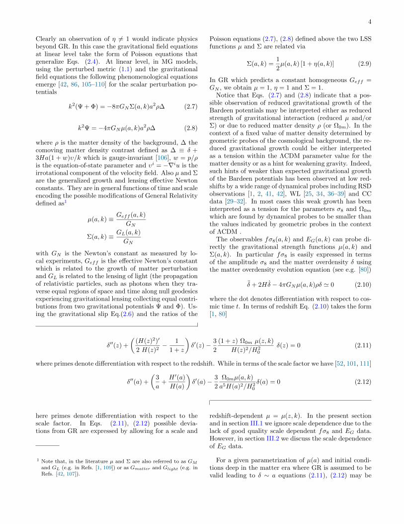
FIG. 1. The fσ8(z) data compilation from Table VI used inthe present analysis. The subset of the data with less corre-lation is indicated with dark red. The red curve shows thePlanck18/ΛCDM prediction (parameter values Ω0m = 0.315,ga = 0, σ8 = 0.811), the blue curve shows the best fitof the fσ8(z) in the context of parametrizations Eq.(2.18)with a ΛCDM background (parameter values Ω0m = 0.272,ga = −1.306, σ8 = 0.886) and the shaded regions correspondto 1σ confidence level around the best fit (see also Table II).

GR-ΛCDM Planck18

Best Fit (Ω0 m=0.313, ga=-0.129, gb=-2.308 , n=2, m=2)

0.0 0.2 0.4 0.6 0.8 1.00.0

0.1

0.2

0.3

0.4

0.5

0.6

0.7

z

EG(z)

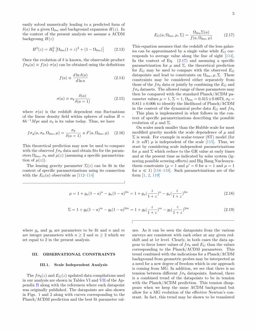
FIG. 2. The EG(z) data compilation from Table VII (scales3 < R < 150h−1Mpc) used in the present analysis. The sub-set of the data with less correlation is indicated with darkred. The red curve shows the theoretical prediction basedon the Planck18/ΛCDM parameter values (Ω0m = 0.315,σ8 = 0.811, µ = 1, Σ = 1), the blue curve shows the bestfit theoretical prediction based on the parametrizations (2.18)and (2.19) with parameter values (Ω0m = 0.313, ga = −0.129,gb = −2.308). Notice that the best fit is significantly belowthe Planck/ΛCDM theoretical prediction and implies weakergravity (µ < 1 and Σ < 1) at the 4.6σ level (see also TableII).

into a trend for lower values for the gravitational pa-rameters µ and Σ and is quantified through a detailedmaximum likelihood analysis.

Each fσ8(z) and EG(z) datapoint of the compilationsof Tables VI and VII has been published separately in thecontext of independent analyses of distinct galaxy sam-ples and lensing data. However, the correlations amongthe datapoints considered due to overlap of the analyzed

galaxy samples may lead to an amplification of the ex-isting trends indicated by the data and an amplificationof the existing tension of the best fit parameters withPlanck/ΛCDM . Despite of this fact we have chosen tokeep the relatively large number of distinct publisheddatapoints in order to maximize the information encodedin the compilations considered keeping in mind that thismay lead to an artificial amplification of the trends thatalready exist in the data.

An additional motivation for keeping the full set ofpublished datapoints is that it is not always clear whichone of the correlated points is more suitable to keep. Ig-noring one of the correlated points arbitrarily or simplybased on time of publication criteria could lead to loss ofuseful information or selection bias.

Keeping the full set of points does not significantlychange the results and the level of tension between thegrowth data best fit parameter values corresponding toMG and Planck/ΛCDM best fit in the context of GR. Inorder to demonstrate the validity of the above reasonswe have repeated our analysis for a subset of the fσ8

and EG data where we have removed most earlier datathat were subject to correlations with more recent dataas indicated with bold font in the index of the Tables VIand VII and as shown in Figs. 1 and 2 with dark red.The result was a data compilation of about half the fσ8and EG datapoints with significantly less correlation.The results of the statistical analysis of this dataset arepresented in Appendix A and indicate a minor reductionof the overall tension.

For the construction of the likelihood contours of themodel parameters in the context of the fσ8 and EGdatasets we construct χ2

fσ8and χ2

EGFor the construc-

tion of χ2fσ8

we use the vector [2]

V ifσ8(zi, p) ≡ fσobs8,i −

fσth8 (zi, p)

q(zi,Ω0m,Ωfid0m)

(3.1)

where fσobs8,i is the the value of the ith datapoint, withi = 1, ..., Nfσ8

(where Nfσ8= 66 corresponds to the total

number of datapoints of Table VI) and fσth8 (zi, p) is thetheoretical prediction, both at redshift zi. The parame-ter vector p corresponds to the parameters σ8,Ω0m, ga ofEq. (2.16) with the parametrization (2.18). The fiducialAlcock-Paczynsk correction factor q [1, 2, 41] is definedas

q(zi,Ω0m,Ωfid0m) =

H(zi)dA(zi)

Hfid(zi)dfidA (zi)

(3.2)

where H(z), dA(z) correspond to the Hubble parameterand the angular diameter distance of the true cosmologyand the superscript fid indicates the fiducial cosmologyused in each survey to convert angles and redshift to dis-tances for evaluating the correlation function. As shownin Table II, the effects of this correction factor are lessthan about 10% in the derived best fit parameter values.

7

Best fit

fσ8 data

Planck ΛCDM

0.1 0.2 0.3 0.4 0.5 0.60.6

0.7

0.8

0.9

1.0

1.1

1.2

Ω0m

σ 8 Best fit

fσ8 data

Planck ΛCDM

0.1 0.2 0.3 0.4 0.5 0.6-3

-2

-1

0

1

2

Ω0m

ga

Best fit

fσ8 data

Planck ΛCDM

-4 -2 0 2 40.4

0.6

0.8

1.0

1.2

1.4

ga

σ 8

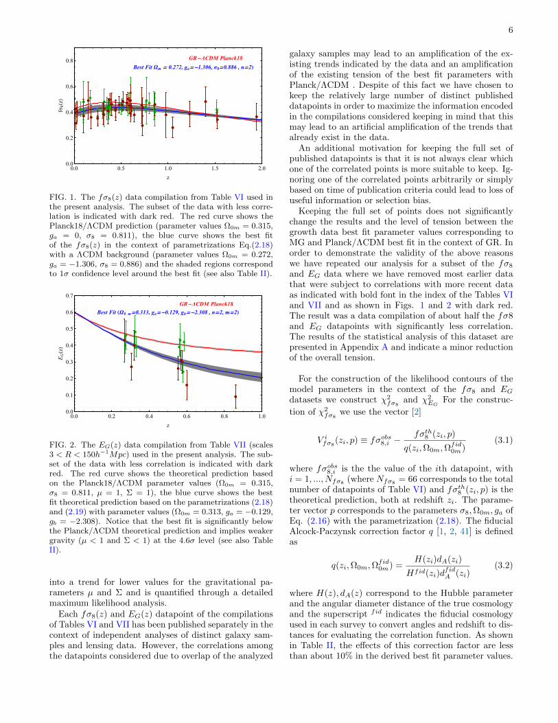
FIG. 3. The three 1σ - 7σ confidence contours in 2D projected parameter spaces of the parameter space (Ω0m, σ8, ga) in thecontext of parametrization Eq.(2.18) with n = 2 including the fiducial correction factor Eq. (3.2). The RSD data fσ8(z) fromTable VI of the Appendix B was used. The third parameter in each contour was fixed to the best fit value. The red and greendots describe the Planck18/ΛCDM best fit and the best-fit values from data.

Best fit

EG (z) data

Planck ΛCDM

0.0 0.1 0.2 0.3 0.4 0.5-6

-4

-2

0

2

Ω0m

ga

Best fit

EG (z) data

Planck ΛCDM

-4 -2 0 2 4-8

-6

-4

-2

0

2

4

ga

gb

Best fit

EG (z) data

Planck ΛCDM

0.0 0.2 0.4 0.6 0.8-8

-6

-4

-2

0

2

4

6

Ω0m

gb

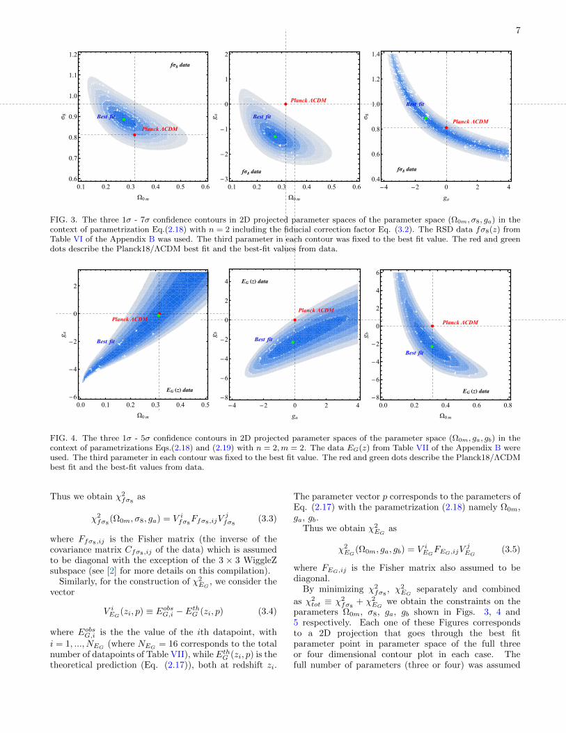
FIG. 4. The three 1σ - 5σ confidence contours in 2D projected parameter spaces of the parameter space (Ω0m, ga, gb) in thecontext of parametrizations Eqs.(2.18) and (2.19) with n = 2,m = 2. The data EG(z) from Table VII of the Appendix B wereused. The third parameter in each contour was fixed to the best fit value. The red and green dots describe the Planck18/ΛCDMbest fit and the best-fit values from data.

Thus we obtain χ2fσ8

as

χ2fσ8

(Ω0m, σ8, ga) = V ifσ8Ffσ8,ijV

jfσ8

(3.3)

where Ffσ8,ij is the Fisher matrix (the inverse of thecovariance matrix Cfσ8,ij of the data) which is assumedto be diagonal with the exception of the 3 × 3 WiggleZsubspace (see [2] for more details on this compilation).

Similarly, for the construction of χ2EG

, we consider thevector

V iEG(zi, p) ≡ EobsG,i − EthG (zi, p) (3.4)

where EobsG,i is the the value of the ith datapoint, with

i = 1, ..., NEG(where NEG

= 16 corresponds to the totalnumber of datapoints of Table VII), while EthG (zi, p) is thetheoretical prediction (Eq. (2.17)), both at redshift zi.

The parameter vector p corresponds to the parameters ofEq. (2.17) with the parametrization (2.18) namely Ω0m,ga, gb.

Thus we obtain χ2EG

as

χ2EG

(Ω0m, ga, gb) = V iEGFEG,ijV

jEG

(3.5)

where FEG,ij is the Fisher matrix also assumed to bediagonal.

By minimizing χ2fσ8

, χ2EG

separately and combined

as χ2tot ≡ χ2

fσ8+ χ2

EGwe obtain the constraints on the

parameters Ω0m, σ8, ga, gb shown in Figs. 3, 4 and5 respectively. Each one of these Figures correspondsto a 2D projection that goes through the best fitparameter point in parameter space of the full threeor four dimensional contour plot in each case. Thefull number of parameters (three or four) was assumed

8

Best fit

EG+ fσ8 data

Planck ΛCDM

0.1 0.2 0.3 0.4 0.50.7

0.8

0.9

1.0

1.1

Ω0m

σ 8

Best fit

EG+ fσ8 data

Planck ΛCDM

0.1 0.2 0.3 0.4 0.5-2.0

-1.5

-1.0

-0.5

0.0

0.5

Ω0m

ga

Best fit

EG+ fσ8 data

Planck ΛCDM

-3 -2 -1 0 1 20.6

0.7

0.8

0.9

1.0

1.1

1.2

ga

σ 8

Best fit

EG+ fσ8 data

Planck ΛCDM

-3 -2 -1 0 1 2-6

-5

-4

-3

-2

-1

0

1

ga

gb Best fit

EG+ fσ8 data

Planck ΛCDM

0.1 0.2 0.3 0.4 0.5-6

-4

-2

0

2

Ω0m

gb

Best fit

EG+ fσ8 data

Planck ΛCDM

-6 -4 -2 0 20.70

0.75

0.80

0.85

0.90

0.95

1.00

gb

σ 8

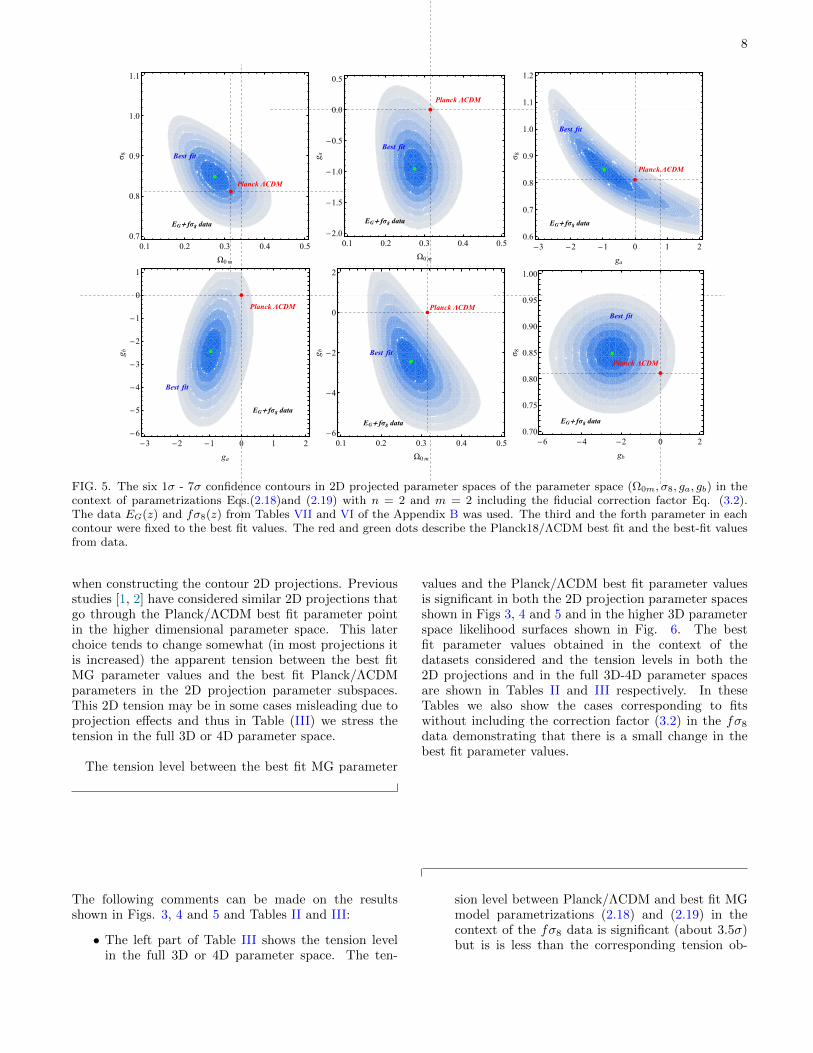
FIG. 5. The six 1σ - 7σ confidence contours in 2D projected parameter spaces of the parameter space (Ω0m, σ8, ga, gb) in thecontext of parametrizations Eqs.(2.18)and (2.19) with n = 2 and m = 2 including the fiducial correction factor Eq. (3.2).The data EG(z) and fσ8(z) from Tables VII and VI of the Appendix B was used. The third and the forth parameter in eachcontour were fixed to the best fit values. The red and green dots describe the Planck18/ΛCDM best fit and the best-fit valuesfrom data.

when constructing the contour 2D projections. Previousstudies [1, 2] have considered similar 2D projections thatgo through the Planck/ΛCDM best fit parameter pointin the higher dimensional parameter space. This laterchoice tends to change somewhat (in most projections itis increased) the apparent tension between the best fitMG parameter values and the best fit Planck/ΛCDMparameters in the 2D projection parameter subspaces.This 2D tension may be in some cases misleading due toprojection effects and thus in Table (III) we stress thetension in the full 3D or 4D parameter space.

The tension level between the best fit MG parameter

values and the Planck/ΛCDM best fit parameter valuesis significant in both the 2D projection parameter spacesshown in Figs 3, 4 and 5 and in the higher 3D parameterspace likelihood surfaces shown in Fig. 6. The bestfit parameter values obtained in the context of thedatasets considered and the tension levels in both the2D projections and in the full 3D-4D parameter spacesare shown in Tables II and III respectively. In theseTables we also show the cases corresponding to fitswithout including the correction factor (3.2) in the fσ8

data demonstrating that there is a small change in thebest fit parameter values.

The following comments can be made on the resultsshown in Figs. 3, 4 and 5 and Tables II and III:

• The left part of Table III shows the tension levelin the full 3D or 4D parameter space. The ten-

sion level between Planck/ΛCDM and best fit MGmodel parametrizations (2.18) and (2.19) in thecontext of the fσ8 data is significant (about 3.5σ)but is is less than the corresponding tension ob-

9

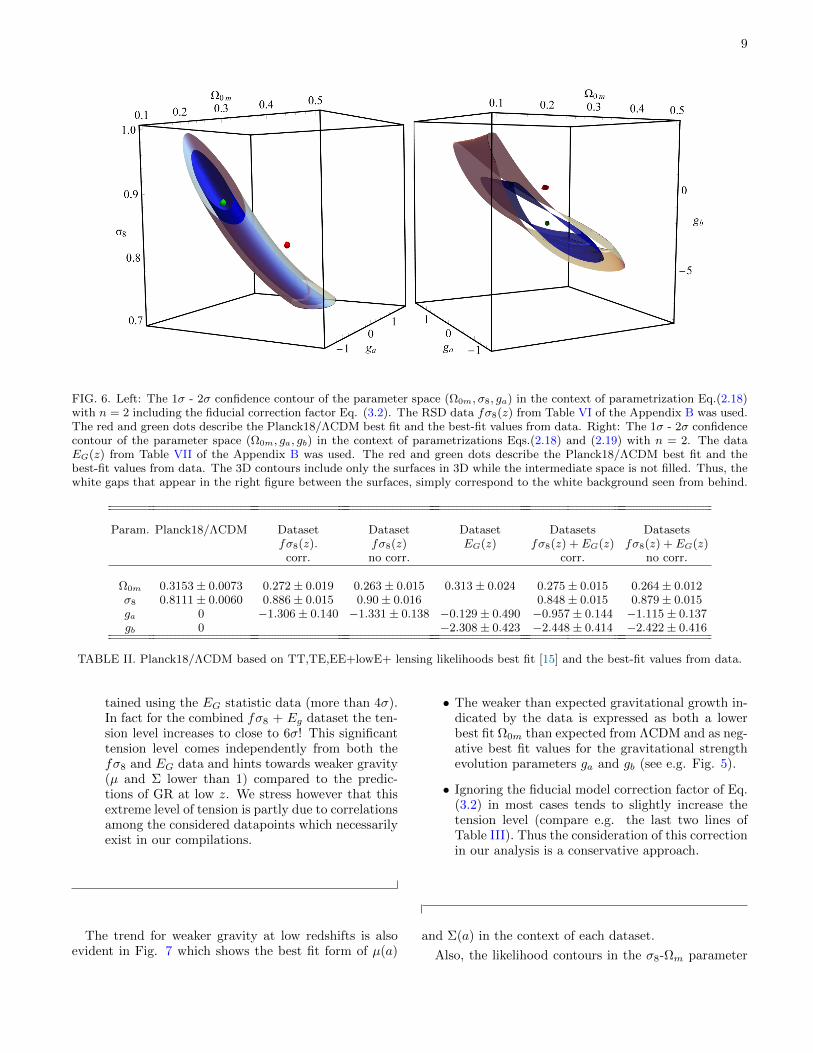
FIG. 6. Left: The 1σ - 2σ confidence contour of the parameter space (Ω0m, σ8, ga) in the context of parametrization Eq.(2.18)with n = 2 including the fiducial correction factor Eq. (3.2). The RSD data fσ8(z) from Table VI of the Appendix B was used.The red and green dots describe the Planck18/ΛCDM best fit and the best-fit values from data. Right: The 1σ - 2σ confidencecontour of the parameter space (Ω0m, ga, gb) in the context of parametrizations Eqs.(2.18) and (2.19) with n = 2. The dataEG(z) from Table VII of the Appendix B was used. The red and green dots describe the Planck18/ΛCDM best fit and thebest-fit values from data. The 3D contours include only the surfaces in 3D while the intermediate space is not filled. Thus, thewhite gaps that appear in the right figure between the surfaces, simply correspond to the white background seen from behind.

Param. Planck18/ΛCDM Dataset Dataset Dataset Datasets Datasetsfσ8(z). fσ8(z) EG(z) fσ8(z) + EG(z) fσ8(z) + EG(z)

corr. no corr. corr. no corr.

Ω0m 0.3153± 0.0073 0.272± 0.019 0.263± 0.015 0.313± 0.024 0.275± 0.015 0.264± 0.012σ8 0.8111± 0.0060 0.886± 0.015 0.90± 0.016 0.848± 0.015 0.879± 0.015ga 0 −1.306± 0.140 −1.331± 0.138 −0.129± 0.490 −0.957± 0.144 −1.115± 0.137gb 0 −2.308± 0.423 −2.448± 0.414 −2.422± 0.416

TABLE II. Planck18/ΛCDM based on TT,TE,EE+lowE+ lensing likelihoods best fit [15] and the best-fit values from data.

tained using the EG statistic data (more than 4σ).In fact for the combined fσ8 + Eg dataset the ten-sion level increases to close to 6σ! This significanttension level comes independently from both thefσ8 and EG data and hints towards weaker gravity(µ and Σ lower than 1) compared to the predic-tions of GR at low z. We stress however that thisextreme level of tension is partly due to correlationsamong the considered datapoints which necessarilyexist in our compilations.

• The weaker than expected gravitational growth in-dicated by the data is expressed as both a lowerbest fit Ω0m than expected from ΛCDM and as neg-ative best fit values for the gravitational strengthevolution parameters ga and gb (see e.g. Fig. 5).

• Ignoring the fiducial model correction factor of Eq.(3.2) in most cases tends to slightly increase thetension level (compare e.g. the last two lines ofTable III). Thus the consideration of this correctionin our analysis is a conservative approach.

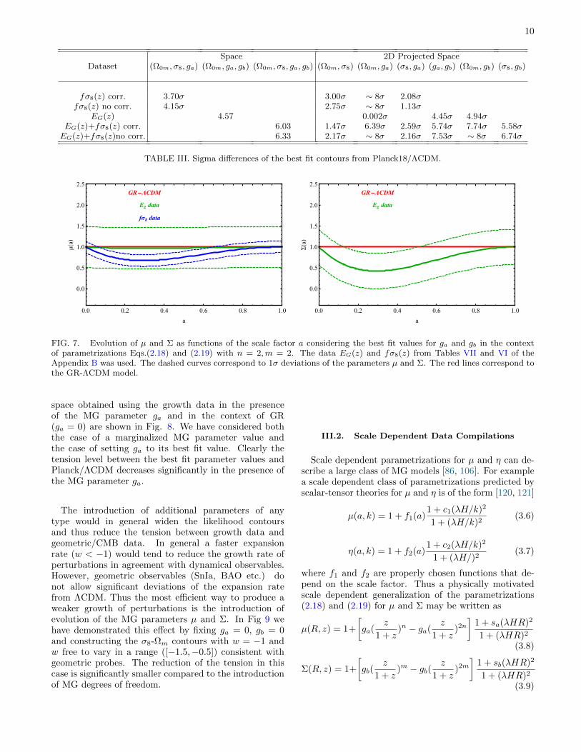
The trend for weaker gravity at low redshifts is alsoevident in Fig. 7 which shows the best fit form of µ(a)

and Σ(a) in the context of each dataset.

Also, the likelihood contours in the σ8-Ωm parameter

10

Space 2D Projected SpaceDataset (Ω0m, σ8, ga) (Ω0m, ga, gb) (Ω0m, σ8, ga, gb) (Ω0m, σ8) (Ω0m, ga) (σ8, ga) (ga, gb) (Ω0m, gb) (σ8, gb)

fσ8(z) corr. 3.70σ 3.00σ ∼ 8σ 2.08σfσ8(z) no corr. 4.15σ 2.75σ ∼ 8σ 1.13σ

EG(z) 4.57 0.002σ 4.45σ 4.94σEG(z)+fσ8(z) corr. 6.03 1.47σ 6.39σ 2.59σ 5.74σ 7.74σ 5.58σEG(z)+fσ8(z)no corr. 6.33 2.17σ ∼ 8σ 2.16σ 7.53σ ∼ 8σ 6.74σ

TABLE III. Sigma differences of the best fit contours from Planck18/ΛCDM.

GR-ΛCDM

fσ8 data

Eg data

0.0 0.2 0.4 0.6 0.8 1.0

0.0

0.5

1.0

1.5

2.0

2.5

a

μ(a)

GR-ΛCDM

Eg data

0.0 0.2 0.4 0.6 0.8 1.0

0.0

0.5

1.0

1.5

2.0

2.5

a

Σ(a)

FIG. 7. Evolution of µ and Σ as functions of the scale factor a considering the best fit values for ga and gb in the contextof parametrizations Eqs.(2.18) and (2.19) with n = 2,m = 2. The data EG(z) and fσ8(z) from Tables VII and VI of theAppendix B was used. The dashed curves correspond to 1σ deviations of the parameters µ and Σ. The red lines correspond tothe GR-ΛCDM model.

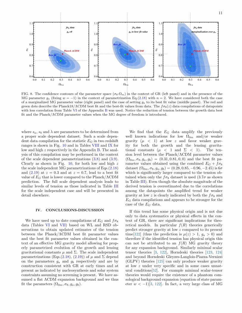
space obtained using the growth data in the presenceof the MG parameter ga and in the context of GR(ga = 0) are shown in Fig. 8. We have considered boththe case of a marginalized MG parameter value andthe case of setting ga to its best fit value. Clearly thetension level between the best fit parameter values andPlanck/ΛCDM decreases significantly in the presence ofthe MG parameter ga.

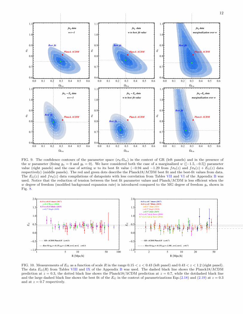
The introduction of additional parameters of anytype would in general widen the likelihood contoursand thus reduce the tension between growth data andgeometric/CMB data. In general a faster expansionrate (w < −1) would tend to reduce the growth rate ofperturbations in agreement with dynamical observables.However, geometric observables (SnIa, BAO etc.) donot allow significant deviations of the expansion ratefrom ΛCDM. Thus the most efficient way to produce aweaker growth of perturbations is the introduction ofevolution of the MG parameters µ and Σ. In Fig 9 wehave demonstrated this effect by fixing ga = 0, gb = 0and constructing the σ8-Ωm contours with w = −1 andw free to vary in a range ([−1.5,−0.5]) consistent withgeometric probes. The reduction of the tension in thiscase is significantly smaller compared to the introductionof MG degrees of freedom.

III.2. Scale Dependent Data Compilations

Scale dependent parametrizations for µ and η can de-scribe a large class of MG models [86, 106]. For examplea scale dependent class of parametrizations predicted byscalar-tensor theories for µ and η is of the form [120, 121]

µ(a, k) = 1 + f1(a)1 + c1(λH/k)2

1 + (λH/k)2(3.6)

η(a, k) = 1 + f2(a)1 + c2(λH/k)2

1 + (λH/)2(3.7)

where f1 and f2 are properly chosen functions that de-pend on the scale factor. Thus a physically motivatedscale dependent generalization of the parametrizations(2.18) and (2.19) for µ and Σ may be written as

µ(R, z) = 1+

[ga(

z

1 + z)n − ga(

z

1 + z)2n

]1 + sa(λHR)2

1 + (λHR)2

(3.8)

Σ(R, z) = 1+

[gb(

z

1 + z)m − gb(

z

1 + z)2m

]1 + sb(λHR)2

1 + (λHR)2

(3.9)

11

Best fit

fσ8 data

ga=0

Planck ΛCDM

0.0 0.1 0.2 0.3 0.4 0.5 0.60.6

0.7

0.8

0.9

1.0

1.1

Ω0m

σ 8

Best fit

fσ8 data

ga to best fit value

Planck ΛCDM

0.0 0.1 0.2 0.3 0.4 0.5 0.60.6

0.7

0.8

0.9

1.0

1.1

Ω0m

σ 8

Best fit

fσ8 data

marginalization over ga

Planck ΛCDM

0.0 0.1 0.2 0.3 0.4 0.5 0.60.6

0.7

0.8

0.9

1.0

1.1

Ω0m

σ 8

FIG. 8. The confidence contours of the parameter space (σ8-Ωm) in the context of GR (left panel) and in the presence of theMG parameter ga (fixing w = −1) in the context of parametrization Eq.(2.18) with n = 2. We have considered both the caseof a marginalized MG parameter value (right panel) and the case of setting ga to its best fit value (middle panel). The red andgreen dots describe the Planck18/ΛCDM best fit and the best-fit values from data. The fσ8(z) data compilations of datapointswith less correlation from Table VI of the Appendix B was used. Notice the reduction of tension between the growth data bestfit and the Planck/ΛCDM parameter values when the MG degree of freedom is introduced.

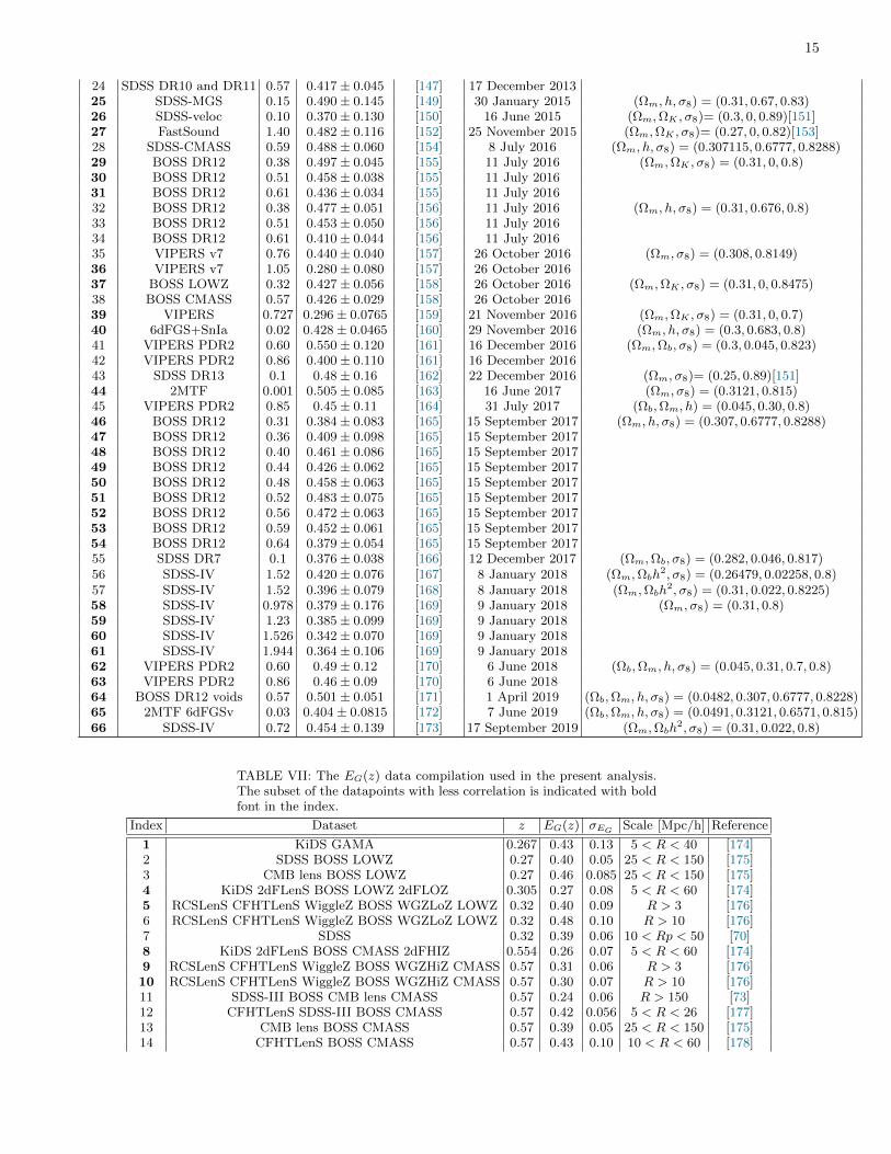
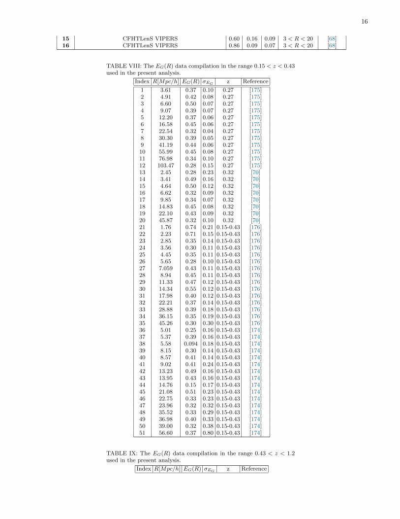
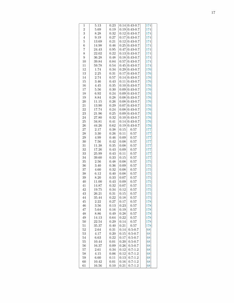
where sa, sb and λ are parameters to be determined froma proper scale dependent dataset. Such a scale depen-dent data compilation for the statistic EG in two redshiftranges is shown in Fig. 10 and in Tables VIII and IX forlow and high z respectively in the Appendix B. The anal-ysis of this compilation may be performed in the contextof the scale dependent parametrizations (3.8) and (3.9).Clearly as shown in Fig. 10, for both low and high zthe scale independent MG parametrizations of Eqs.(2.18)and (2.19) at z = 0.3 and at z = 0.7, lead to a best fitvalue of EG that is lower compared to the Planck/ΛCDMprediction. The full scale dependent analysis leads tosimilar levels of tension as those indicated in Table IIIfor the scale independent case and will be presented indetail elsewhere.

IV. CONCLUSIONS-DISCUSSION

We have used up to date compilations of EG and fσ8

data (Tables VI and VII) based on WL and RSD ob-servations to obtain updated estimates of the tensionbetween the Planck/ΛCDM best fit parameter valuesand the best fit parameter values obtained in the con-text of an effective MG gravity model allowing for prop-erly parametrized evolution of the growth and lensinggravitational constants µ and Σ. The scale independentparametrizations (Eqs.(2.18), (2.19)) of µ and Σ dependon the parameters ga and gb respectively and are byconstruction consistent with GR at early times and atpresent as indicated by nucleosynthesis and solar systemconstraints assuming no screening is present. We have as-sumed a flat ΛCDM expansion background and we thusfit the parameters (Ω0m, σ8, ga, gb).

We find that the EG data amplify the previouslywell known indications for low Ω0m and/or weakergravity (µ < 1) at low z and favor weaker grav-ity for both the growth and the lensing gravita-tional constants (µ < 1 and Σ < 1). The ten-sion level between the Planck/ΛCDM parameter values(Ω0m, σ8, ga, gb) = (0.31, 0.81, 0, 0) and the best fit pa-rameter values obtained using the combined EG + fσ8

dataset (Ω0m, σ8, ga, gb) = (0.28, 0.85,−0.96,−2.45) is 6σwhich is significantly larger compared to the tension ob-tained when only the fσ8 dataset is used (3.7σ as shownin Table III). Even though the absolute magnitude of thederived tension is overestimated due to the correlationsamong the datapoints the amplified trend for weakergravity at low z is clearly indicated by both the fσ8 andEG data compilations and appears to be stronger for thecase of the EG data.

If this trend has some physical origin and is not dueonly to data systematics or physical effects in the con-text of GR, there are significant implications for theo-retical models. In particular f(R) theories genericallypredict stronger gravity at low z compared to its presenttime[122] (thus the prediction is µ(z) > 1, ga > 0) andtherefore if the identified tension has physical origin thiscan not be attributed to an f(R) MG gravity theoryfor any expansion background. Similarly minimal scalartensor theories [3, 122], Horndeski theories [123, 124]and beyond Horndeski Gleyzes-Langlois-Piazza-Vernizzi(GLPV) theories [125] can only produce weaker gravityat low z under very specific and in some cases unnat-ural conditions[52]. For example minimal scalar-tensortheories would require the existence of a phantom com-sological background expansion (equation of state param-eter w < −1)[3, 122]. In fact, a very large class of MG

12

Best fit

fσ8 data

w=-1

Planck ΛCDM

0.0 0.1 0.2 0.3 0.4 0.5 0.60.6

0.7

0.8

0.9

1.0

1.1

Ω0m

σ 8

Best fit

fσ8 data

w to best fit value

Planck ΛCDM

0.0 0.1 0.2 0.3 0.4 0.5 0.60.6

0.7

0.8

0.9

1.0

1.1

Ω0m

σ 8

Best fit

fσ8 data

marginalization over w

Planck ΛCDM

0.0 0.1 0.2 0.3 0.4 0.5 0.60.6

0.7

0.8

0.9

1.0

1.1

Ω0m

σ 8

Best fit

fσ8 - Eg data

w=-1

Planck ΛCDM

0.0 0.1 0.2 0.3 0.4 0.5 0.60.6

0.7

0.8

0.9

1.0

1.1

Ω0m

σ 8

Best fit

fσ8 - Eg data

w to best fit value

Planck ΛCDM

0.0 0.1 0.2 0.3 0.4 0.5 0.60.6

0.7

0.8

0.9

1.0

1.1

Ω0m

σ 8

Best fit

fσ8-Eg data

marginalization over w

Planck ΛCDM

0.0 0.1 0.2 0.3 0.4 0.5 0.60.6

0.7

0.8

0.9

1.0

1.1

Ω0m

σ 8FIG. 9. The confidence contours of the parameter space (σ8-Ωm) in the context of GR (left panels) and in the presence ofthe w parameter (fixing ga = 0 and gb = 0). We have considered both the case of a marginalized w ([−1.5,−0.5]) parametervalue (right panels) and the case of setting w to its best fit value (−0.94 and −1.29 from fσ8(z) and fσ8(z) + EG(z) datarespectively) (middle panels). The red and green dots describe the Planck18/ΛCDM best fit and the best-fit values from data.The EG(z) and fσ8(z) data compilations of datapoints with less correlation from Tables VII and VI of the Appendix B wasused. Notice that the reduction of tension between the best fit parameter values and Planck/ΛCDM is less efficient when thew degree of freedom (modified background expansion rate) is introduced compared to the MG degree of freedom ga shown inFig. 8.

0.15<z<0.43 Amon (2017)

z=0.32 Reyes (2010)

0.15<z<0.43 Blake (2015)

z=0.27 Singh (2018)

– – – GR-ΛCDM Planck18 (z=0.3)

· - · Best Fit (ga=-0.129, gb=-2.308, n=2, m=2, z=0.3)

1 5 10 50 100-1.0

-0.5

0.0

0.5

1.0

1.5

2.0

R [Mpc/h]

EG

0.43<z<0.7 Amon (2017)

z=0.57 Alam (2016)

0.5<z<0.7 de la Torre (2016)

0.7<z<1.2 de la Torre (2016)

0.43<z<0.7 Blake (2015)

z=0.57 Jullo (2019)

z=0.57 Singh (2018)

· · · GR-ΛCDM Planck18 (z=0.7)

——— Best Fit (ga=-0.129, gb=-2.308 , n=2, m=2, z=0.7)

1 2 5 10 20 50-1.0

-0.5

0.0

0.5

1.0

1.5

2.0

R [Mpc/h]

EG

FIG. 10. Measurements of EG as a function of scale R in the range 0.15 < z < 0.43 (left panel) and 0.43 < z < 1.2 (right panel).The data EG(R) from Tables VIII and IX of the Appendix B was used. The dashed black line shows the Planck18/ΛCDMprediction at z = 0.3, the dotted black line shows the Planck18/ΛCDM prediction at z = 0.7, while the dotdashed black lineand the large dashed black line shows the best fit of the EG in the context of parametrizations Eqs.(2.18) and (2.19) at z = 0.3and at z = 0.7 respectively.

13

Param. Planck18/ΛCDM Dataset Dataset Dataset Datasets Datasetsfσ8(z). fσ8(z) EG(z) fσ8(z) + EG(z) fσ8(z) + EG(z)

corr. no corr. corr. no corr.

Ω0m 0.3153± 0.0073 0.289± 0.032 0.283± 0.028 0.285± 0.044 0.288± 0.026 0.282± 0.023σ8 0.8111± 0.0060 0.807± 0.024 0.819± 0.025 0.795± 0.024 0.810± 0.024ga 0 −0.767± 0.299 −0.826± 0.293 −0.621± 0.914 −0.627± 0.291 −0.723± 0.281gb 0 −3.510± 0.605 −3.562± 0.601 −3.563± 0.601

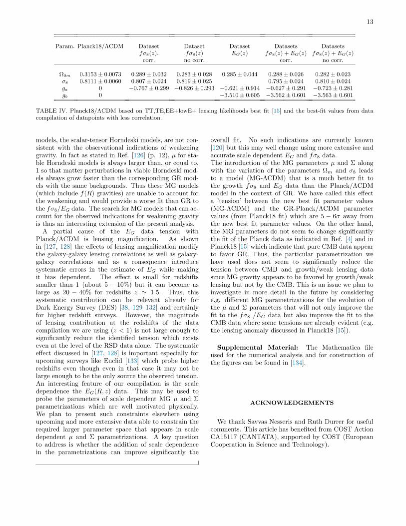
TABLE IV. Planck18/ΛCDM based on TT,TE,EE+lowE+ lensing likelihoods best fit [15] and the best-fit values from datacompilation of datapoints with less correlation.

models, the scalar-tensor Horndeski models, are not con-sistent with the observational indications of weakeninggravity. In fact as stated in Ref. [126] (p. 12), µ for sta-ble Horndeski models is always larger than, or equal to,1 so that matter perturbations in viable Horndeski mod-els always grow faster than the corresponding GR mod-els with the same backgrounds. Thus these MG models(which include f(R) gravities) are unable to account forthe weakening and would provide a worse fit than GR tothe fσ8/EG data. The search for MG models that can ac-count for the observed indications for weakening gravityis thus an interesting extension of the present analysis.

A partial cause of the EG data tension withPlanck/ΛCDM is lensing magnification. As shownin [127, 128] the effects of lensing magnification modifythe galaxy-galaxy lensing correlations as well as galaxy-galaxy correlations and as a consequence introducesystematic errors in the estimate of EG while makingit bias dependent. The effect is small for redshiftssmaller than 1 (about 5 − 10%) but it can become aslarge as 20 − 40% for redshifts z ' 1.5. Thus, thissystematic contribution can be relevant already forDark Energy Survey (DES) [38, 129–132] and certainlyfor higher redshift surveys. However, the magnitudeof lensing contribution at the redshifts of the datacompilation we are using (z < 1) is not large enough tosignificantly reduce the identified tension which existseven at the level of the RSD data alone. The systematiceffect discussed in [127, 128] is important especially forupcoming surveys like Euclid [133] which probe higherredshifts even though even in that case it may not belarge enough to be the only source the observed tension.An interesting feature of our compilation is the scaledependence the EG(R, z) data. This may be used toprobe the parameters of scale dependent MG µ and Σparametrizations which are well motivated physically.We plan to present such constraints elsewhere usingupcoming and more extensive data able to constrain therequired larger parameter space that appears in scaledependent µ and Σ parametrizations. A key questionto address is whether the addition of scale dependencein the parametrizations can improve significantly the

overall fit. No such indications are currently known[120] but this may well change using more extensive andaccurate scale dependent EG and fσ8 data.The introduction of the MG parameters µ and Σ alongwith the variation of the parameters Ωm and σ8 leadsto a model (MG-ΛCDM) that is a much better fit tothe growth fσ8 and EG data than the Planck/ΛCDMmodel in the context of GR. We have called this effecta ’tension’ between the new best fit parameter values(MG-ΛCDM) and the GR-Planck/ΛCDM parametervalues (from Planck18 fit) which are 5 − 6σ away fromthe new best fit parameter values. On the other hand,the MG parameters do not seem to change significantlythe fit of the Planck data as indicated in Ref. [4] and inPlanck18 [15] which indicate that pure CMB data appearto favor GR. Thus, the particular parametrization wehave used does not seem to significantly reduce thetension between CMB and growth/weak lensing datasince MG gravity appears to be favored by growth/weaklensing but not by the CMB. This is an issue we plan toinvestigate in more detail in the future by consideringe.g. different MG parametrizations for the evolution ofthe µ and Σ parameters that will not only improve thefit to the fσ8 /EG data but also improve the fit to theCMB data where some tensions are already evident (e.g.the lensing anomaly discussed in Planck18 [15]).

Supplemental Material: The Mathematica fileused for the numerical analysis and for construction ofthe figures can be found in [134].

ACKNOWLEDGEMENTS

We thank Savvas Nesseris and Ruth Durrer for usefulcomments. This article has benefited from COST ActionCA15117 (CANTATA), supported by COST (EuropeanCooperation in Science and Technology).

14

Space 2D Projected SpaceDataset (Ω0m, σ8, ga) (Ω0m, ga, gb) (Ω0m, σ8, ga, gb) (Ω0m, σ8) (Ω0m, ga) (σ8, ga) (ga, gb) (Ω0m, gb) (σ8, gb)

fσ8(z) corr. 2.39σ 0.22σ 2.19σ 1.79σfσ8(z) no corr. 2.55σ 0.19σ 2.19σ 1.48σ

EG(z) 5.06 0.01σ 4.04σ 6.28σEG(z)+fσ8(z) corr. 5.69 0.36σ 1.35σ 1.59σ 4.31σ 6.12σ 5.12σEG(z)+fσ8(z)no corr. 5.78 0.31σ 2.21σ 1.33σ 4.54σ 6.38σ 5.29σ

TABLE V. Sigma differences of the best fit contours from Planck18/ΛCDM. The EG(z) and fσ8(z) data compilations ofdatapoints with less correlation from Tables VII and VI of the Appendix B was used.

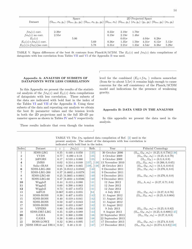
Appendix A: ANALYSIS OF SUBSETS OFDATAPOINTS WITH LESS CORRELATION

In this Appendix we present the results of the statisti-cal analysis of the fσ8(z) and EG(z) data compilationsof datapoints with less correlation. These subsets ofthe data are indicated with bold font in the index ofthe Tables VI and VII of the Appendix B. Using thesesubsets of the data and repeating our analysis we obtainthe best fit parameter values and the tension levelsin both the 2D projections and in the full 3D-4D pa-rameter spaces as shown in Tables IV and V respectively.

These results indicate that even though the tension

level for the combined (EG+fσ8 ) reduces somewhat(from 6σ to about 5.5σ) it remains high enough to causeconcerns for the self consistency of the Planck/ΛCDMmodel and indications for the presence of weakeninggravity.

Appendix B: DATA USED IN THE ANALYSIS

In this appendix we present the data used in theanalysis.

TABLE VI: The fσ8 updated data compilation of Ref. [2] used in thepresent analysis. The subset of the datapoints with less correlation isindicated with bold font in the index.

Index Dataset z fσ8(z) Refs. Year Fiducial Cosmology

1 SDSS-LRG 0.35 0.440± 0.050 [135] 30 October 2006 (Ωm,ΩK , σ8)= (0.25, 0, 0.756)[136]2 VVDS 0.77 0.490± 0.18 [135] 6 October 2009 (Ωm,ΩK , σ8) = (0.25, 0, 0.78)3 2dFGRS 0.17 0.510± 0.060 [135] 6 October 2009 (Ωm,ΩK) = (0.3, 0, 0.9)4 2MRS 0.02 0.314± 0.048 [137], [138] 13 November 2010 (Ωm,ΩK , σ8) = (0.266, 0, 0.65)5 SnIa+IRAS 0.02 0.398± 0.065 [139], [138] 20 October 2011 (Ωm,ΩK , σ8) = (0.3, 0, 0.814)6 SDSS-LRG-200 0.25 0.3512± 0.0583 [140] 9 December 2011 (Ωm,ΩK , σ8) = (0.276, 0, 0.8)7 SDSS-LRG-200 0.37 0.4602± 0.0378 [140] 9 December 20118 SDSS-LRG-60 0.25 0.3665± 0.0601 [140] 9 December 2011 (Ωm,ΩK , σ8) = (0.276, 0, 0.8)9 SDSS-LRG-60 0.37 0.4031± 0.0586 [140] 9 December 2011

10 WiggleZ 0.44 0.413± 0.080 [141] 12 June 2012 (Ωm, h, σ8) = (0.27, 0.71, 0.8)11 WiggleZ 0.60 0.390± 0.063 [141] 12 June 201212 WiggleZ 0.73 0.437± 0.072 [141] 12 June 201213 6dFGS 0.067 0.423± 0.055 [84] 4 July 2012 (Ωm,ΩK , σ8) = (0.27, 0, 0.76)14 SDSS-BOSS 0.30 0.407± 0.055 [142] 11 August 2012 (Ωm,ΩK , σ8) = (0.25, 0, 0.804)15 SDSS-BOSS 0.40 0.419± 0.041 [142] 11 August 201216 SDSS-BOSS 0.50 0.427± 0.043 [142] 11 August 201217 SDSS-BOSS 0.60 0.433± 0.067 [142] 11 August 201218 VIPERS 0.80 0.470± 0.080 [143] 9 July 2013 (Ωm,ΩK , σ8) = (0.25, 0, 0.82)19 SDSS-DR7-LRG 0.35 0.429± 0.089 [144] 8 August 2013 (Ωm,ΩK , σ8)= (0.25, 0, 0.809)[145]20 GAMA 0.18 0.360± 0.090 [146] 22 September 2013 (Ωm,ΩK , σ8) = (0.27, 0, 0.8)21 GAMA 0.38 0.440± 0.060 [146] 22 September 201322 BOSS-LOWZ 0.32 0.384± 0.095 [147] 17 December 2013 (Ωm,ΩK , σ8) = (0.274, 0, 0.8)23 SDSS DR10 and DR11 0.32 0.48± 0.10 [147] 17 December 2013 (Ωm,ΩK , σ8)= (0.274, 0, 0.8)[148]

15

24 SDSS DR10 and DR11 0.57 0.417± 0.045 [147] 17 December 201325 SDSS-MGS 0.15 0.490± 0.145 [149] 30 January 2015 (Ωm, h, σ8) = (0.31, 0.67, 0.83)26 SDSS-veloc 0.10 0.370± 0.130 [150] 16 June 2015 (Ωm,ΩK , σ8)= (0.3, 0, 0.89)[151]27 FastSound 1.40 0.482± 0.116 [152] 25 November 2015 (Ωm,ΩK , σ8)= (0.27, 0, 0.82)[153]28 SDSS-CMASS 0.59 0.488± 0.060 [154] 8 July 2016 (Ωm, h, σ8) = (0.307115, 0.6777, 0.8288)29 BOSS DR12 0.38 0.497± 0.045 [155] 11 July 2016 (Ωm,ΩK , σ8) = (0.31, 0, 0.8)30 BOSS DR12 0.51 0.458± 0.038 [155] 11 July 201631 BOSS DR12 0.61 0.436± 0.034 [155] 11 July 201632 BOSS DR12 0.38 0.477± 0.051 [156] 11 July 2016 (Ωm, h, σ8) = (0.31, 0.676, 0.8)33 BOSS DR12 0.51 0.453± 0.050 [156] 11 July 201634 BOSS DR12 0.61 0.410± 0.044 [156] 11 July 201635 VIPERS v7 0.76 0.440± 0.040 [157] 26 October 2016 (Ωm, σ8) = (0.308, 0.8149)36 VIPERS v7 1.05 0.280± 0.080 [157] 26 October 201637 BOSS LOWZ 0.32 0.427± 0.056 [158] 26 October 2016 (Ωm,ΩK , σ8) = (0.31, 0, 0.8475)38 BOSS CMASS 0.57 0.426± 0.029 [158] 26 October 201639 VIPERS 0.727 0.296± 0.0765 [159] 21 November 2016 (Ωm,ΩK , σ8) = (0.31, 0, 0.7)40 6dFGS+SnIa 0.02 0.428± 0.0465 [160] 29 November 2016 (Ωm, h, σ8) = (0.3, 0.683, 0.8)41 VIPERS PDR2 0.60 0.550± 0.120 [161] 16 December 2016 (Ωm,Ωb, σ8) = (0.3, 0.045, 0.823)42 VIPERS PDR2 0.86 0.400± 0.110 [161] 16 December 201643 SDSS DR13 0.1 0.48± 0.16 [162] 22 December 2016 (Ωm, σ8)= (0.25, 0.89)[151]44 2MTF 0.001 0.505± 0.085 [163] 16 June 2017 (Ωm, σ8) = (0.3121, 0.815)45 VIPERS PDR2 0.85 0.45± 0.11 [164] 31 July 2017 (Ωb,Ωm, h) = (0.045, 0.30, 0.8)46 BOSS DR12 0.31 0.384± 0.083 [165] 15 September 2017 (Ωm, h, σ8) = (0.307, 0.6777, 0.8288)47 BOSS DR12 0.36 0.409± 0.098 [165] 15 September 201748 BOSS DR12 0.40 0.461± 0.086 [165] 15 September 201749 BOSS DR12 0.44 0.426± 0.062 [165] 15 September 201750 BOSS DR12 0.48 0.458± 0.063 [165] 15 September 201751 BOSS DR12 0.52 0.483± 0.075 [165] 15 September 201752 BOSS DR12 0.56 0.472± 0.063 [165] 15 September 201753 BOSS DR12 0.59 0.452± 0.061 [165] 15 September 201754 BOSS DR12 0.64 0.379± 0.054 [165] 15 September 201755 SDSS DR7 0.1 0.376± 0.038 [166] 12 December 2017 (Ωm,Ωb, σ8) = (0.282, 0.046, 0.817)56 SDSS-IV 1.52 0.420± 0.076 [167] 8 January 2018 (Ωm,Ωbh

2, σ8) = (0.26479, 0.02258, 0.8)57 SDSS-IV 1.52 0.396± 0.079 [168] 8 January 2018 (Ωm,Ωbh

2, σ8) = (0.31, 0.022, 0.8225)58 SDSS-IV 0.978 0.379± 0.176 [169] 9 January 2018 (Ωm, σ8) = (0.31, 0.8)59 SDSS-IV 1.23 0.385± 0.099 [169] 9 January 201860 SDSS-IV 1.526 0.342± 0.070 [169] 9 January 201861 SDSS-IV 1.944 0.364± 0.106 [169] 9 January 201862 VIPERS PDR2 0.60 0.49± 0.12 [170] 6 June 2018 (Ωb,Ωm, h, σ8) = (0.045, 0.31, 0.7, 0.8)63 VIPERS PDR2 0.86 0.46± 0.09 [170] 6 June 201864 BOSS DR12 voids 0.57 0.501± 0.051 [171] 1 April 2019 (Ωb,Ωm, h, σ8) = (0.0482, 0.307, 0.6777, 0.8228)65 2MTF 6dFGSv 0.03 0.404± 0.0815 [172] 7 June 2019 (Ωb,Ωm, h, σ8) = (0.0491, 0.3121, 0.6571, 0.815)66 SDSS-IV 0.72 0.454± 0.139 [173] 17 September 2019 (Ωm,Ωbh

2, σ8) = (0.31, 0.022, 0.8)

TABLE VII: The EG(z) data compilation used in the present analysis.The subset of the datapoints with less correlation is indicated with boldfont in the index.

Index Dataset z EG(z) σEG Scale [Mpc/h] Reference

1 KiDS GAMA 0.267 0.43 0.13 5 < R < 40 [174]2 SDSS BOSS LOWZ 0.27 0.40 0.05 25 < R < 150 [175]3 CMB lens BOSS LOWZ 0.27 0.46 0.085 25 < R < 150 [175]4 KiDS 2dFLenS BOSS LOWZ 2dFLOZ 0.305 0.27 0.08 5 < R < 60 [174]5 RCSLenS CFHTLenS WiggleZ BOSS WGZLoZ LOWZ 0.32 0.40 0.09 R > 3 [176]6 RCSLenS CFHTLenS WiggleZ BOSS WGZLoZ LOWZ 0.32 0.48 0.10 R > 10 [176]7 SDSS 0.32 0.39 0.06 10 < Rp < 50 [70]8 KiDS 2dFLenS BOSS CMASS 2dFHIZ 0.554 0.26 0.07 5 < R < 60 [174]9 RCSLenS CFHTLenS WiggleZ BOSS WGZHiZ CMASS 0.57 0.31 0.06 R > 3 [176]10 RCSLenS CFHTLenS WiggleZ BOSS WGZHiZ CMASS 0.57 0.30 0.07 R > 10 [176]11 SDSS-III BOSS CMB lens CMASS 0.57 0.24 0.06 R > 150 [73]12 CFHTLenS SDSS-III BOSS CMASS 0.57 0.42 0.056 5 < R < 26 [177]13 CMB lens BOSS CMASS 0.57 0.39 0.05 25 < R < 150 [175]14 CFHTLenS BOSS CMASS 0.57 0.43 0.10 10 < R < 60 [178]

16

15 CFHTLenS VIPERS 0.60 0.16 0.09 3 < R < 20 [68]16 CFHTLenS VIPERS 0.86 0.09 0.07 3 < R < 20 [68]

TABLE VIII: The EG(R) data compilation in the range 0.15 < z < 0.43used in the present analysis.

Index R[Mpc/h] EG(R) σEG z Reference

1 3.61 0.37 0.10 0.27 [175]2 4.91 0.42 0.08 0.27 [175]3 6.60 0.50 0.07 0.27 [175]4 9.07 0.39 0.07 0.27 [175]5 12.20 0.37 0.06 0.27 [175]6 16.58 0.45 0.06 0.27 [175]7 22.54 0.32 0.04 0.27 [175]8 30.30 0.39 0.05 0.27 [175]9 41.19 0.44 0.06 0.27 [175]10 55.99 0.45 0.08 0.27 [175]11 76.98 0.34 0.10 0.27 [175]12 103.47 0.28 0.15 0.27 [175]13 2.45 0.28 0.23 0.32 [70]14 3.41 0.49 0.16 0.32 [70]15 4.64 0.50 0.12 0.32 [70]16 6.62 0.32 0.09 0.32 [70]17 9.85 0.34 0.07 0.32 [70]18 14.83 0.45 0.08 0.32 [70]19 22.10 0.43 0.09 0.32 [70]20 45.87 0.32 0.10 0.32 [70]21 1.76 0.74 0.21 0.15-0.43 [176]22 2.23 0.71 0.15 0.15-0.43 [176]23 2.85 0.35 0.14 0.15-0.43 [176]24 3.56 0.30 0.11 0.15-0.43 [176]25 4.45 0.35 0.11 0.15-0.43 [176]26 5.65 0.28 0.10 0.15-0.43 [176]27 7.059 0.43 0.11 0.15-0.43 [176]28 8.94 0.45 0.11 0.15-0.43 [176]29 11.33 0.47 0.12 0.15-0.43 [176]30 14.34 0.55 0.12 0.15-0.43 [176]31 17.98 0.40 0.12 0.15-0.43 [176]32 22.21 0.37 0.14 0.15-0.43 [176]33 28.88 0.39 0.18 0.15-0.43 [176]34 36.15 0.35 0.19 0.15-0.43 [176]35 45.26 0.30 0.30 0.15-0.43 [176]36 5.01 0.25 0.16 0.15-0.43 [174]37 5.37 0.39 0.16 0.15-0.43 [174]38 5.58 0.094 0.18 0.15-0.43 [174]39 8.15 0.30 0.14 0.15-0.43 [174]40 8.57 0.41 0.14 0.15-0.43 [174]41 9.02 0.41 0.24 0.15-0.43 [174]42 13.23 0.49 0.16 0.15-0.43 [174]43 13.95 0.43 0.16 0.15-0.43 [174]44 14.76 0.15 0.17 0.15-0.43 [174]45 21.08 0.51 0.23 0.15-0.43 [174]46 22.75 0.33 0.23 0.15-0.43 [174]47 23.96 0.32 0.32 0.15-0.43 [174]48 35.52 0.33 0.29 0.15-0.43 [174]49 36.98 0.40 0.33 0.15-0.43 [174]50 39.00 0.32 0.38 0.15-0.43 [174]51 56.60 0.37 0.80 0.15-0.43 [174]

TABLE IX: The EG(R) data compilation in the range 0.43 < z < 1.2used in the present analysis.

Index R[Mpc/h] EG(R) σEG z Reference

17

1 5.13 0.23 0.14 0.43-0.7 [174]2 5.69 0.19 0.19 0.43-0.7 [174]3 8.28 0.32 0.12 0.43-0.7 [174]4 9.19 0.27 0.17 0.43-0.7 [174]5 13.69 0.21 0.12 0.43-0.7 [174]6 14.98 0.46 0.25 0.43-0.7 [174]7 24.43 0.95 0.47 0.43-0.7 [174]8 22.02 0.22 0.13 0.43-0.7 [174]9 36.28 0.48 0.18 0.43-0.7 [174]10 39.84 0.84 0.57 0.43-0.7 [174]11 59.78 0.54 0.45 0.43-0.7 [174]12 1.74 0.34 0.29 0.43-0.7 [176]13 2.25 0.31 0.17 0.43-0.7 [176]14 2.74 0.57 0.14 0.43-0.7 [176]15 3.46 0.43 0.11 0.43-0.7 [176]16 4.45 0.35 0.10 0.43-0.7 [176]17 5.56 0.30 0.09 0.43-0.7 [176]18 6.92 0.24 0.09 0.43-0.7 [176]19 8.84 0.28 0.08 0.43-0.7 [176]20 11.15 0.26 0.08 0.43-0.7 [176]21 13.90 0.29 0.07 0.43-0.7 [176]22 17.74 0.24 0.08 0.43-0.7 [176]23 21.96 0.25 0.09 0.43-0.7 [176]24 27.80 0.32 0.10 0.43-0.7 [176]25 34.81 0.41 0.14 0.43-0.7 [176]26 44.26 0.62 0.19 0.43-0.7 [176]27 2.17 0.38 0.15 0.57 [177]28 3.30 0.26 0.11 0.57 [177]29 4.99 0.46 0.09 0.57 [177]30 7.56 0.42 0.08 0.57 [177]31 11.38 0.35 0.08 0.57 [177]32 17.26 0.43 0.09 0.57 [177]33 25.99 0.43 0.11 0.57 [177]34 39.60 0.33 0.15 0.57 [177]35 2.56 0.48 0.08 0.57 [175]36 3.40 0.36 0.09 0.57 [175]37 4.60 0.32 0.08 0.57 [175]38 6.12 0.40 0.08 0.57 [175]39 8.20 0.33 0.07 0.57 [175]40 11.00 0.43 0.09 0.57 [175]41 14.87 0.32 0.07 0.57 [175]42 19.75 0.34 0.12 0.57 [175]43 26.21 0.31 0.15 0.57 [175]44 35.44 0.22 0.18 0.57 [175]45 2.22 0.27 0.17 0.57 [178]46 3.56 0.13 0.23 0.57 [178]47 5.64 0.16 0.19 0.57 [178]48 8.86 0.49 0.28 0.57 [178]49 14.13 0.64 0.22 0.57 [178]50 22.54 0.29 0.14 0.57 [178]51 35.37 0.40 0.21 0.57 [178]52 2.64 0.31 0.14 0.5-0.7 [68]53 4.17 0.20 0.15 0.5-0.7 [68]54 6.63 0.22 0.17 0.5-0.7 [68]55 10.44 0.01 0.20 0.5-0.7 [68]56 16.37 0.09 0.26 0.5-0.7 [68]57 2.61 0.34 0.12 0.7-1.2 [68]58 4.15 0.06 0.12 0.7-1.2 [68]59 6.60 0.11 0.13 0.7-1.2 [68]60 10.42 0.01 0.16 0.7-1.2 [68]61 16.56 0.10 0.21 0.7-1.2 [68]

18

[1] Savvas Nesseris, George Pantazis, and LeandrosPerivolaropoulos, “Tension and constraints on modi-fied gravity parametrizations of Geff(z) from growthrate and Planck data,” Phys. Rev. D96, 023542 (2017),arXiv:1703.10538 [astro-ph.CO].

[2] Lavrentios Kazantzidis and Leandros Perivolaropoulos,“Evolution of the fσ8 tension with the Planck15/ΛCDMdetermination and implications for modified grav-ity theories,” Phys. Rev. D97, 103503 (2018),arXiv:1803.01337 [astro-ph.CO].

[3] Leandros Perivolaropoulos and Lavrentios Kazantzidis,“Hints of modified gravity in cosmos and in thelab?” Int. J. Mod. Phys. D28, 1942001 (2019),arXiv:1904.09462 [gr-qc].

[4] Lavrentios Kazantzidis and Leandros Perivolaropou-los, “Is gravity getting weaker at low z? Observa-tional evidence and theoretical implications,” (2019),arXiv:1907.03176 [astro-ph.CO].

[5] Sean M. Carroll, “The Cosmological constant,” LivingRev. Rel. 4, 1 (2001), arXiv:astro-ph/0004075 [astro-ph].

[6] Clifford M. Will, “The Confrontation between GeneralRelativity and Experiment,” Living Rev. Rel. 17, 4(2014), arXiv:1403.7377 [gr-qc].

[7] Adam G. Riess et al. (Supernova Search Team), “Ob-servational evidence from supernovae for an acceleratinguniverse and a cosmological constant,” Astron. J. 116,1009–1038 (1998), arXiv:astro-ph/9805201 [astro-ph].

[8] S. Perlmutter et al. (Supernova Cosmology Project),“Measurements of Ω and Λ from 42 high redshift super-novae,” Astrophys. J. 517, 565–586 (1999), arXiv:astro-ph/9812133 [astro-ph].

[9] Steven Weinberg, “The Cosmological Constant Prob-lem,” Rev. Mod. Phys. 61, 1–23 (1989).

[10] Jerome Martin, “Everything You Always Wanted ToKnow About The Cosmological Constant Problem (ButWere Afraid To Ask),” Comptes Rendus Physique 13,566–665 (2012), arXiv:1205.3365 [astro-ph.CO].

[11] C. P. Burgess, “The Cosmological Constant Problem:Why it’s hard to get Dark Energy from Micro-physics,”in Proceedings, 100th Les Houches Summer School:Post-Planck Cosmology: Les Houches, France, July 8- August 2, 2013 (2015) pp. 149–197, arXiv:1309.4133[hep-th].

[12] P. J. Steinhardt, “Cosmological Challenges for the 21stCentury,” in Critical Problems in Physics, edited byV. L. Fitch, D. R. Marlow, and M. A. E. Dementi(1997) p. 123.

[13] H. E. S. Velten, R. F. vom Marttens, and W. Zimdahl,“Aspects of the cosmological “coincidence problem”,”Eur. Phys. J. C74, 3160 (2014), arXiv:1410.2509 [astro-ph.CO].

[14] P. A. R. Ade et al. (Planck), “Planck 2015 results.XIII. Cosmological parameters,” Astron. Astrophys.594, A13 (2016), arXiv:1502.01589 [astro-ph.CO].

[15] N. Aghanim et al. (Planck), “Planck 2018 results. VI.Cosmological parameters,” (2018), arXiv:1807.06209[astro-ph.CO].

[16] Adam G. Riess et al., “A 2.4% Determination of the Lo-cal Value of the Hubble Constant,” Astrophys. J. 826,56 (2016), arXiv:1604.01424 [astro-ph.CO].

[17] Adam G. Riess et al., “Milky Way Cepheid Standardsfor Measuring Cosmic Distances and Application toGaia DR2: Implications for the Hubble Constant,” As-trophys. J. 861, 126 (2018), arXiv:1804.10655 [astro-ph.CO].

[18] S. Birrer et al., “H0LiCOW - IX. Cosmographic analysisof the doubly imaged quasar SDSS 1206+4332 and anew measurement of the Hubble constant,” Mon. Not.Roy. Astron. Soc. 484, 4726 (2019), arXiv:1809.01274[astro-ph.CO].

[19] Gong-Bo Zhao, Levon Pogosian, Alessandra Silvestri,and Joel Zylberberg, “Searching for modified growthpatterns with tomographic surveys,” Phys. Rev. D79,083513 (2009), arXiv:0809.3791 [astro-ph].

[20] Yan-Chuan Cai and Gary Bernstein, “Combining weaklensing tomography and spectroscopic redshift surveys,”Mon. Not. Roy. Astron. Soc. 422, 1045–1056 (2012),arXiv:1112.4478 [astro-ph.CO].

[21] Shahab Joudaki and Manoj Kaplinghat, “Dark En-ergy and Neutrino Masses from Future Measurementsof the Expansion History and Growth of Structure,”Phys. Rev. D86, 023526 (2012), arXiv:1106.0299 [astro-ph.CO].

[22] Ismael Tereno, Elisabetta Semboloni, and Tim Schrab-back, “COSMOS weak-lensing constraints on modi-fied gravity,” Astron. Astrophys. 530, A68 (2011),arXiv:1012.5854 [astro-ph.CO].

[23] Fergus Simpson et al., “CFHTLenS: Testing the Laws ofGravity with Tomographic Weak Lensing and RedshiftSpace Distortions,” Mon. Not. Roy. Astron. Soc. 429,2249 (2013), arXiv:1212.3339 [astro-ph.CO].

[24] Gongbo Zhao, David Bacon, Roy Maartens, Mario San-tos, and Alvise Raccanelli, “Model-independent con-straints on dark energy and modified gravity with theSKA,” Proceedings, Advancing Astrophysics with theSquare Kilometre Array (AASKA14): Giardini Naxos,Italy, June 9-13, 2014, PoS AASKA14, 165 (2015).

[25] Shahab Joudaki et al., “KiDS-450 + 2dFLenS: Cos-mological parameter constraints from weak gravita-tional lensing tomography and overlapping redshift-space galaxy clustering,” Mon. Not. Roy. Astron.Soc. 474, 4894–4924 (2018), arXiv:1707.06627 [astro-ph.CO].

[26] Edmund Bertschinger, “On the Growth of Perturba-tions as a Test of Dark Energy,” Astrophys. J. 648,797–806 (2006), arXiv:astro-ph/0604485 [astro-ph].

[27] S. Nesseris and Leandros Perivolaropoulos, “Cross-ing the Phantom Divide: Theoretical Implicationsand Observational Status,” JCAP 0701, 018 (2007),arXiv:astro-ph/0610092 [astro-ph].

[28] Spyros Basilakos, Savvas Nesseris, and LeandrosPerivolaropoulos, “Observational constraints on vi-able f(R) parametrizations with geometrical and dy-namical probes,” Phys. Rev. D87, 123529 (2013),arXiv:1302.6051 [astro-ph.CO].

[29] Eduardo J. Ruiz and Dragan Huterer, “Testing thedark energy consistency with geometry and growth,”Phys. Rev. D91, 063009 (2015), arXiv:1410.5832 [astro-ph.CO].

[30] Eduardo Rozo et al. (DSDD), “Cosmological Con-straints from the SDSS maxBCG Cluster Catalog,” As-

19

trophys. J. 708, 645–660 (2010), arXiv:0902.3702 [astro-ph.CO].

[31] David Rapetti, Steven W. Allen, Adam Mantz, andHarald Ebeling, “Constraints on modified gravity fromthe observed X-ray luminosity function of galaxy clus-ters,” Mon. Not. Roy. Astron. Soc. 400, 699 (2009),arXiv:0812.2259 [astro-ph].

[32] S. Bocquet et al. (SPT), “Mass Calibration and Cosmo-logical Analysis of the SPT-SZ Galaxy Cluster SampleUsing Velocity Dispersion σv and X-ray YX Measure-ments,” Astrophys. J. 799, 214 (2015), arXiv:1407.2942[astro-ph.CO].

[33] Fabian Schmidt, “Weak Lensing Probes of Mod-ified Gravity,” Phys. Rev. D78, 043002 (2008),arXiv:0805.4812 [astro-ph].

[34] H. Hildebrandt et al., “KiDS-450: Cosmological param-eter constraints from tomographic weak gravitationallensing,” Mon. Not. Roy. Astron. Soc. 465, 1454 (2017),arXiv:1606.05338 [astro-ph.CO].

[35] Catherine Heymans et al., “CFHTLenS: The Canada-France-Hawaii Telescope Lensing Survey,” Mon. Not.Roy. Astron. Soc. 427, 146 (2012), arXiv:1210.0032[astro-ph.CO].

[36] M. A. Troxel et al. (DES), “Dark Energy Survey Year 1results: Cosmological constraints from cosmic shear,”Phys. Rev. D98, 043528 (2018), arXiv:1708.01538[astro-ph.CO].

[37] F. Kohlinger et al., “KiDS-450: The tomographic weaklensing power spectrum and constraints on cosmologicalparameters,” Mon. Not. Roy. Astron. Soc. 471, 4412–4435 (2017), arXiv:1706.02892 [astro-ph.CO].

[38] T. M. C. Abbott et al. (DES), “Dark Energy Surveyyear 1 results: Cosmological constraints from galaxyclustering and weak lensing,” Phys. Rev. D98, 043526(2018), arXiv:1708.01530 [astro-ph.CO].

[39] T. M. C. Abbott et al. (DES), “Dark Energy SurveyYear 1 Results: Constraints on Extended Cosmolog-ical Models from Galaxy Clustering and Weak Lens-ing,” Phys. Rev. D99, 123505 (2019), arXiv:1810.02499[astro-ph.CO].

[40] Lado Samushia et al., “The Clustering of Galaxies in theSDSS-III DR9 Baryon Oscillation Spectroscopic Survey:Testing Deviations from Λ and General Relativity us-ing anisotropic clustering of galaxies,” Mon. Not. Roy.Astron. Soc. 429, 1514–1528 (2013), arXiv:1206.5309[astro-ph.CO].

[41] Edward Macaulay, Ingunn Kathrine Wehus, andHans Kristian Eriksen, “Lower Growth Rate from Re-cent Redshift Space Distortion Measurements than Ex-pected from Planck,” Phys. Rev. Lett. 111, 161301(2013), arXiv:1303.6583 [astro-ph.CO].

[42] Andrew Johnson, Chris Blake, Jason Dossett, JunKoda, David Parkinson, and Shahab Joudaki, “Search-ing for Modified Gravity: Scale and Redshift De-pendent Constraints from Galaxy Peculiar Velocities,”Mon. Not. Roy. Astron. Soc. 458, 2725–2744 (2016),arXiv:1504.06885 [astro-ph.CO].

[43] Suresh Kumar and Rafael C. Nunes, “Probing the in-teraction between dark matter and dark energy in thepresence of massive neutrinos,” Phys. Rev. D94, 123511(2016), arXiv:1608.02454 [astro-ph.CO].

[44] Alkistis Pourtsidou and Thomas Tram, “ReconcilingCMB and structure growth measurements with darkenergy interactions,” Phys. Rev. D94, 043518 (2016),

arXiv:1604.04222 [astro-ph.CO].[45] Bruno J. Barros, Luca Amendola, Tiago Barreiro, and

Nelson J. Nunes, “Coupled quintessence with a ΛCDMbackground: removing the σ8 tension,” JCAP 1901,007 (2019), arXiv:1802.09216 [astro-ph.CO].

[46] Stefano Camera, Matteo Martinelli, and DanieleBertacca, “Does quartessence ease cosmic tensions?”Phys. Dark Univ. 23, 100247 (2019), arXiv:1704.06277[astro-ph.CO].

[47] Weiqiang Yang, Supriya Pan, Eleonora Di Valentino,Emmanuel N. Saridakis, and Subenoy Chakraborty,“Observational constraints on one-parameter dynam-ical dark-energy parametrizations and the H0 ten-sion,” Phys. Rev. D99, 043543 (2019), arXiv:1810.05141[astro-ph.CO].

[48] Gaetano Lambiase, Subhendra Mohanty, AshishNarang, and Priyank Parashari, “Testing dark energymodels in the light of σ8 tension,” Eur. Phys. J. C79,141 (2019), arXiv:1804.07154 [astro-ph.CO].

[49] Adria Gomez-Valent and Joan Sola, “Relaxing the σ8-tension through running vacuum in the Universe,” EPL120, 39001 (2017), arXiv:1711.00692 [astro-ph.CO].

[50] Adria Gomez-Valent and Joan Sola, “Density pertur-bations for running vacuum: a successful approach tostructure formation and to the σ8-tension,” (2018),arXiv:1801.08501 [astro-ph.CO].

[51] Ana Diaz Rivero, V. Miranda, and Cora Dvorkin,“Observable Predictions for Massive-Neutrino Cosmolo-gies with Model-Independent Dark Energy,” Phys. Rev.D100, 063504 (2019), arXiv:1903.03125 [astro-ph.CO].

[52] Shinji Tsujikawa, “Matter density perturbations and ef-fective gravitational constant in modified gravity mod-els of dark energy,” Phys. Rev. D76, 023514 (2007),arXiv:0705.1032 [astro-ph].

[53] Wayne Hu and Ignacy Sawicki, “Models of f(R) Cos-mic Acceleration that Evade Solar-System Tests,” Phys.Rev. D76, 064004 (2007), arXiv:0705.1158 [astro-ph].

[54] R. Gannouji, B. Moraes, and D. Polarski, “The growthof matter perturbations in f(R) models,” JCAP 0902,034 (2009), arXiv:0809.3374 [astro-ph].

[55] Salvatore Capozziello and Mariafelicia De Laurentis,“Extended Theories of Gravity,” Phys. Rept. 509, 167–321 (2011), arXiv:1108.6266 [gr-qc].

[56] Timothy Clifton, Pedro G. Ferreira, Antonio Padilla,and Constantinos Skordis, “Modified Gravityand Cosmology,” Phys. Rept. 513, 1–189 (2012),arXiv:1106.2476 [astro-ph.CO].

[57] Shin’ichi Nojiri and Sergei D. Odintsov, “Unified cos-mic history in modified gravity: from F(R) theory toLorentz non-invariant models,” Phys. Rept. 505, 59–144 (2011), arXiv:1011.0544 [gr-qc].

[58] Lotfi Boubekeur, Elena Giusarma, Olga Mena, andHector Ramırez, “Current status of modified gravity,”Phys. Rev. D90, 103512 (2014), arXiv:1407.6837 [astro-ph.CO].

[59] Yi-Fu Cai, Chunlong Li, Emmanuel N. Saridakis,and Lingqin Xue, “f(T ) gravity after GW170817and GRB170817A,” Phys. Rev. D97, 103513 (2018),arXiv:1801.05827 [gr-qc].

[60] Judit Perez-Romero and Savvas Nesseris, “Cosmolog-ical constraints and comparison of viable f(R) mod-els,” Phys. Rev. D97, 023525 (2018), arXiv:1710.05634[astro-ph.CO].

[61] S. Nojiri, S. D. Odintsov, and V. K. Oikonomou,

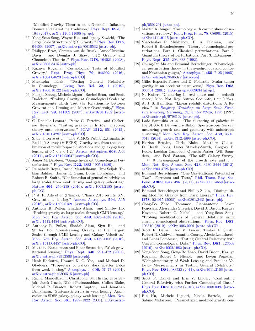
20

“Modified Gravity Theories on a Nutshell: Inflation,Bounce and Late-time Evolution,” Phys. Rept. 692, 1–104 (2017), arXiv:1705.11098 [gr-qc].

[62] Yong-Seon Song, Wayne Hu, and Ignacy Sawicki, “TheLarge Scale Structure of f(R) Gravity,” Phys. Rev. D75,044004 (2007), arXiv:astro-ph/0610532 [astro-ph].

[63] Philippe Brax, Carsten van de Bruck, Anne-ChristineDavis, and Douglas J. Shaw, “f(R) Gravity andChameleon Theories,” Phys. Rev. D78, 104021 (2008),arXiv:0806.3415 [astro-ph].

[64] Kazuya Koyama, “Cosmological Tests of ModifiedGravity,” Rept. Prog. Phys. 79, 046902 (2016),arXiv:1504.04623 [astro-ph.CO].

[65] Mustapha Ishak, “Testing General Relativityin Cosmology,” Living Rev. Rel. 22, 1 (2019),arXiv:1806.10122 [astro-ph.CO].

[66] Pengjie Zhang, Michele Liguori, Rachel Bean, and ScottDodelson, “Probing Gravity at Cosmological Scales byMeasurements which Test the Relationship betweenGravitational Lensing and Matter Overdensity,” Phys.Rev. Lett. 99, 141302 (2007), arXiv:0704.1932 [astro-ph].

[67] C. Danielle Leonard, Pedro G. Ferreira, and Cather-ine Heymans, “Testing gravity with EG: mappingtheory onto observations,” JCAP 1512, 051 (2015),arXiv:1510.04287 [astro-ph.CO].

[68] S. de la Torre et al., “The VIMOS Public ExtragalacticRedshift Survey (VIPERS). Gravity test from the com-bination of redshift-space distortions and galaxy-galaxylensing at 0.5 < z < 1.2,” Astron. Astrophys. 608, A44(2017), arXiv:1612.05647 [astro-ph.CO].

[69] James M. Bardeen, “Gauge Invariant Cosmological Per-turbations,” Phys. Rev. D22, 1882–1905 (1980).

[70] Reinabelle Reyes, Rachel Mandelbaum, Uros Seljak, To-bias Baldauf, James E. Gunn, Lucas Lombriser, andRobert E. Smith, “Confirmation of general relativity onlarge scales from weak lensing and galaxy velocities,”Nature 464, 256–258 (2010), arXiv:1003.2185 [astro-ph.CO].

[71] P. A. R. Ade et al. (Planck), “Planck 2015 results. XV.Gravitational lensing,” Astron. Astrophys. 594, A15(2016), arXiv:1502.01591 [astro-ph.CO].

[72] Anthony R. Pullen, Shadab Alam, and Shirley Ho,“Probing gravity at large scales through CMB lensing,”Mon. Not. Roy. Astron. Soc. 449, 4326–4335 (2015),arXiv:1412.4454 [astro-ph.CO].

[73] Anthony R. Pullen, Shadab Alam, Siyu He, andShirley Ho, “Constraining Gravity at the LargestScales through CMB Lensing and Galaxy Velocities,”Mon. Not. Roy. Astron. Soc. 460, 4098–4108 (2016),arXiv:1511.04457 [astro-ph.CO].

[74] Matthias Bartelmann and Peter Schneider, “Weak grav-itational lensing,” Phys. Rept. 340, 291–472 (2001),arXiv:astro-ph/9912508 [astro-ph].

[75] Henk Hoekstra, Howard K. C. Yee, and Michael D.Gladders, “Properties of galaxy dark matter halosfrom weak lensing,” Astrophys. J. 606, 67–77 (2004),arXiv:astro-ph/0306515 [astro-ph].

[76] Rachel Mandelbaum, Christopher M. Hirata, Uros Sel-jak, Jacek Guzik, Nikhil Padmanabhan, Cullen Blake,Michael R. Blanton, Robert Lupton, and JonathanBrinkmann, “Systematic errors in weak lensing: Appli-cation to SDSS galaxy-galaxy weak lensing,” Mon. Not.Roy. Astron. Soc. 361, 1287–1322 (2005), arXiv:astro-

ph/0501201 [astro-ph].[77] Martin Kilbinger, “Cosmology with cosmic shear obser-

vations: a review,” Rept. Prog. Phys. 78, 086901 (2015),arXiv:1411.0115 [astro-ph.CO].

[78] Viatcheslav F. Mukhanov, H. A. Feldman, andRobert H. Brandenberger, “Theory of cosmological per-turbations. Part 1. Classical perturbations. Part 2.Quantum theory of perturbations. Part 3. Extensions,”Phys. Rept. 215, 203–333 (1992).

[79] Chung-Pei Ma and Edmund Bertschinger, “Cosmologi-cal perturbation theory in the synchronous and confor-mal Newtonian gauges,” Astrophys. J. 455, 7–25 (1995),arXiv:astro-ph/9506072 [astro-ph].

[80] Gilles Esposito-Farese and D. Polarski, “Scalar tensorgravity in an accelerating universe,” Phys. Rev. D63,063504 (2001), arXiv:gr-qc/0009034 [gr-qc].

[81] N. Kaiser, “Clustering in real space and in redshiftspace,” Mon. Not. Roy. Astron. Soc. 227, 1–27 (1987).

[82] A. J. S. Hamilton, “Linear redshift distortions: A Re-view,” in Ringberg Workshop on Large Scale Struc-ture Ringberg, Germany, September 23-28, 1996 (1997)arXiv:astro-ph/9708102 [astro-ph].

[83] Lado Samushia et al., “The clustering of galaxies inthe SDSS-III Baryon Oscillation Spectroscopic Survey:measuring growth rate and geometry with anisotropicclustering,” Mon. Not. Roy. Astron. Soc. 439, 3504–3519 (2014), arXiv:1312.4899 [astro-ph.CO].

[84] Florian Beutler, Chris Blake, Matthew Colless,D. Heath Jones, Lister Staveley-Smith, Gregory B.Poole, Lachlan Campbell, Quentin Parker, Will Saun-ders, and Fred Watson, “The 6dF Galaxy Survey:z ≈ 0 measurement of the growth rate and σ8,”Mon. Not. Roy. Astron. Soc. 423, 3430–3444 (2012),arXiv:1204.4725 [astro-ph.CO].

[85] Edmund Bertschinger, “One Gravitational Potential orTwo? Forecasts and Tests,” Phil. Trans. Roy. Soc.Lond. A369, 4947–4961 (2011), arXiv:1111.4659 [astro-ph.CO].

[86] Edmund Bertschinger and Phillip Zukin, “Distinguish-ing Modified Gravity from Dark Energy,” Phys. Rev.D78, 024015 (2008), arXiv:0801.2431 [astro-ph].

[87] Gong-Bo Zhao, Tommaso Giannantonio, LevonPogosian, Alessandra Silvestri, David J. Bacon, KazuyaKoyama, Robert C. Nichol, and Yong-Seon Song,“Probing modifications of General Relativity usingcurrent cosmological observations,” Phys. Rev. D81,103510 (2010), arXiv:1003.0001 [astro-ph.CO].

[88] Scott F. Daniel, Eric V. Linder, Tristan L. Smith,Robert R. Caldwell, Asantha Cooray, Alexie Leauthaud,and Lucas Lombriser, “Testing General Relativity withCurrent Cosmological Data,” Phys. Rev. D81, 123508(2010), arXiv:1002.1962 [astro-ph.CO].

[89] Yong-Seon Song, Gong-Bo Zhao, David Bacon, KazuyaKoyama, Robert C. Nichol, and Levon Pogosian,“Complementarity of Weak Lensing and Peculiar Ve-locity Measurements in Testing General Relativity,”Phys. Rev. D84, 083523 (2011), arXiv:1011.2106 [astro-ph.CO].

[90] Scott F. Daniel and Eric V. Linder, “ConfrontingGeneral Relativity with Further Cosmological Data,”Phys. Rev. D82, 103523 (2010), arXiv:1008.0397 [astro-ph.CO].

[91] Bin Hu, Michele Liguori, Nicola Bartolo, andSabino Matarrese, “Parametrized modified gravity con-

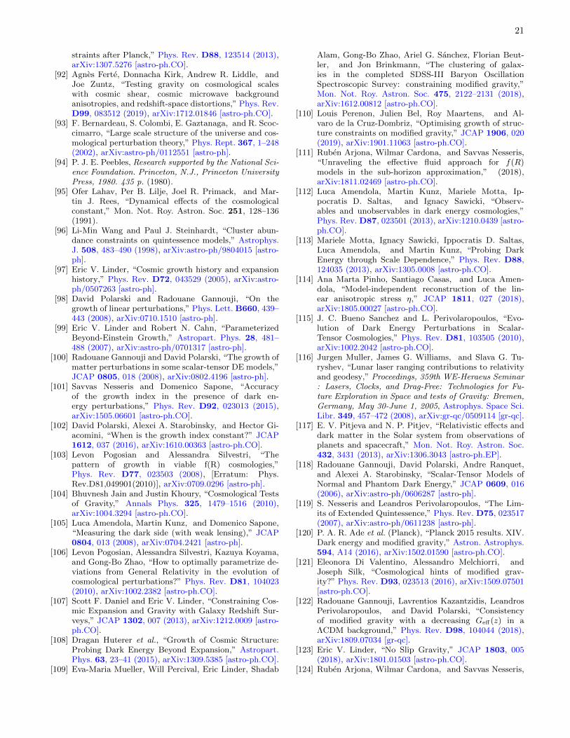
21

straints after Planck,” Phys. Rev. D88, 123514 (2013),arXiv:1307.5276 [astro-ph.CO].

[92] Agnes Ferte, Donnacha Kirk, Andrew R. Liddle, andJoe Zuntz, “Testing gravity on cosmological scaleswith cosmic shear, cosmic microwave backgroundanisotropies, and redshift-space distortions,” Phys. Rev.D99, 083512 (2019), arXiv:1712.01846 [astro-ph.CO].

[93] F. Bernardeau, S. Colombi, E. Gaztanaga, and R. Scoc-cimarro, “Large scale structure of the universe and cos-mological perturbation theory,” Phys. Rept. 367, 1–248(2002), arXiv:astro-ph/0112551 [astro-ph].

[94] P. J. E. Peebles, Research supported by the National Sci-ence Foundation. Princeton, N.J., Princeton UniversityPress, 1980. 435 p. (1980).

[95] Ofer Lahav, Per B. Lilje, Joel R. Primack, and Mar-tin J. Rees, “Dynamical effects of the cosmologicalconstant,” Mon. Not. Roy. Astron. Soc. 251, 128–136(1991).

[96] Li-Min Wang and Paul J. Steinhardt, “Cluster abun-dance constraints on quintessence models,” Astrophys.J. 508, 483–490 (1998), arXiv:astro-ph/9804015 [astro-ph].

[97] Eric V. Linder, “Cosmic growth history and expansionhistory,” Phys. Rev. D72, 043529 (2005), arXiv:astro-ph/0507263 [astro-ph].

[98] David Polarski and Radouane Gannouji, “On thegrowth of linear perturbations,” Phys. Lett. B660, 439–443 (2008), arXiv:0710.1510 [astro-ph].

[99] Eric V. Linder and Robert N. Cahn, “ParameterizedBeyond-Einstein Growth,” Astropart. Phys. 28, 481–488 (2007), arXiv:astro-ph/0701317 [astro-ph].

[100] Radouane Gannouji and David Polarski, “The growth ofmatter perturbations in some scalar-tensor DE models,”JCAP 0805, 018 (2008), arXiv:0802.4196 [astro-ph].

[101] Savvas Nesseris and Domenico Sapone, “Accuracyof the growth index in the presence of dark en-ergy perturbations,” Phys. Rev. D92, 023013 (2015),arXiv:1505.06601 [astro-ph.CO].

[102] David Polarski, Alexei A. Starobinsky, and Hector Gi-acomini, “When is the growth index constant?” JCAP1612, 037 (2016), arXiv:1610.00363 [astro-ph.CO].

[103] Levon Pogosian and Alessandra Silvestri, “Thepattern of growth in viable f(R) cosmologies,”Phys. Rev. D77, 023503 (2008), [Erratum: Phys.Rev.D81,049901(2010)], arXiv:0709.0296 [astro-ph].

[104] Bhuvnesh Jain and Justin Khoury, “Cosmological Testsof Gravity,” Annals Phys. 325, 1479–1516 (2010),arXiv:1004.3294 [astro-ph.CO].

[105] Luca Amendola, Martin Kunz, and Domenico Sapone,“Measuring the dark side (with weak lensing),” JCAP0804, 013 (2008), arXiv:0704.2421 [astro-ph].

[106] Levon Pogosian, Alessandra Silvestri, Kazuya Koyama,and Gong-Bo Zhao, “How to optimally parametrize de-viations from General Relativity in the evolution ofcosmological perturbations?” Phys. Rev. D81, 104023(2010), arXiv:1002.2382 [astro-ph.CO].

[107] Scott F. Daniel and Eric V. Linder, “Constraining Cos-mic Expansion and Gravity with Galaxy Redshift Sur-veys,” JCAP 1302, 007 (2013), arXiv:1212.0009 [astro-ph.CO].

[108] Dragan Huterer et al., “Growth of Cosmic Structure:Probing Dark Energy Beyond Expansion,” Astropart.Phys. 63, 23–41 (2015), arXiv:1309.5385 [astro-ph.CO].

[109] Eva-Maria Mueller, Will Percival, Eric Linder, Shadab

Alam, Gong-Bo Zhao, Ariel G. Sanchez, Florian Beut-ler, and Jon Brinkmann, “The clustering of galax-ies in the completed SDSS-III Baryon OscillationSpectroscopic Survey: constraining modified gravity,”Mon. Not. Roy. Astron. Soc. 475, 2122–2131 (2018),arXiv:1612.00812 [astro-ph.CO].

[110] Louis Perenon, Julien Bel, Roy Maartens, and Al-varo de la Cruz-Dombriz, “Optimising growth of struc-ture constraints on modified gravity,” JCAP 1906, 020(2019), arXiv:1901.11063 [astro-ph.CO].

[111] Ruben Arjona, Wilmar Cardona, and Savvas Nesseris,“Unraveling the effective fluid approach for f(R)models in the sub-horizon approximation,” (2018),arXiv:1811.02469 [astro-ph.CO].

[112] Luca Amendola, Martin Kunz, Mariele Motta, Ip-pocratis D. Saltas, and Ignacy Sawicki, “Observ-ables and unobservables in dark energy cosmologies,”Phys. Rev. D87, 023501 (2013), arXiv:1210.0439 [astro-ph.CO].

[113] Mariele Motta, Ignacy Sawicki, Ippocratis D. Saltas,Luca Amendola, and Martin Kunz, “Probing DarkEnergy through Scale Dependence,” Phys. Rev. D88,124035 (2013), arXiv:1305.0008 [astro-ph.CO].

[114] Ana Marta Pinho, Santiago Casas, and Luca Amen-dola, “Model-independent reconstruction of the lin-ear anisotropic stress η,” JCAP 1811, 027 (2018),arXiv:1805.00027 [astro-ph.CO].

[115] J. C. Bueno Sanchez and L. Perivolaropoulos, “Evo-lution of Dark Energy Perturbations in Scalar-Tensor Cosmologies,” Phys. Rev. D81, 103505 (2010),arXiv:1002.2042 [astro-ph.CO].

[116] Jurgen Muller, James G. Williams, and Slava G. Tu-ryshev, “Lunar laser ranging contributions to relativityand geodesy,” Proceedings, 359th WE-Heraeus Seminar: Lasers, Clocks, and Drag-Free: Technologies for Fu-ture Exploration in Space and tests of Gravity: Bremen,Germany, May 30-June 1, 2005, Astrophys. Space Sci.Libr. 349, 457–472 (2008), arXiv:gr-qc/0509114 [gr-qc].

[117] E. V. Pitjeva and N. P. Pitjev, “Relativistic effects anddark matter in the Solar system from observations ofplanets and spacecraft,” Mon. Not. Roy. Astron. Soc.432, 3431 (2013), arXiv:1306.3043 [astro-ph.EP].

[118] Radouane Gannouji, David Polarski, Andre Ranquet,and Alexei A. Starobinsky, “Scalar-Tensor Models ofNormal and Phantom Dark Energy,” JCAP 0609, 016(2006), arXiv:astro-ph/0606287 [astro-ph].

[119] S. Nesseris and Leandros Perivolaropoulos, “The Lim-its of Extended Quintessence,” Phys. Rev. D75, 023517(2007), arXiv:astro-ph/0611238 [astro-ph].

[120] P. A. R. Ade et al. (Planck), “Planck 2015 results. XIV.Dark energy and modified gravity,” Astron. Astrophys.594, A14 (2016), arXiv:1502.01590 [astro-ph.CO].

[121] Eleonora Di Valentino, Alessandro Melchiorri, andJoseph Silk, “Cosmological hints of modified grav-ity?” Phys. Rev. D93, 023513 (2016), arXiv:1509.07501[astro-ph.CO].

[122] Radouane Gannouji, Lavrentios Kazantzidis, LeandrosPerivolaropoulos, and David Polarski, “Consistencyof modified gravity with a decreasing Geff(z) in aΛCDM background,” Phys. Rev. D98, 104044 (2018),arXiv:1809.07034 [gr-qc].

[123] Eric V. Linder, “No Slip Gravity,” JCAP 1803, 005(2018), arXiv:1801.01503 [astro-ph.CO].

[124] Ruben Arjona, Wilmar Cardona, and Savvas Nesseris,

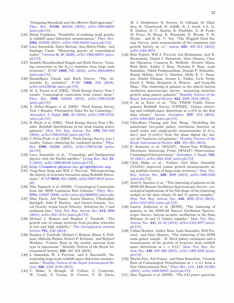
22

“Designing Horndeski and the effective fluid approach,”Phys. Rev. D100, 063526 (2019), arXiv:1904.06294[astro-ph.CO].

[125] Shinji Tsujikawa, “Possibility of realizing weak gravityin redshift space distortion measurements,” Phys. Rev.D92, 044029 (2015), arXiv:1505.02459 [astro-ph.CO].

[126] Luca Amendola, Dario Bettoni, Ana Marta Pinho, andSantiago Casas, “Measuring gravity at cosmologicalscales,” Universe 6, 20 (2020), arXiv:1902.06978 [astro-ph.CO].

[127] Azadeh Moradinezhad Dizgah and Ruth Durrer, “Lens-ing corrections to the Eg(z) statistics from large scalestructure,” JCAP 1609, 035 (2016), arXiv:1604.08914[astro-ph.CO].

[128] Basundhara Ghosh and Ruth Durrer, “The ob-servable Eg statistics,” JCAP 1906, 010 (2019),arXiv:1812.09546 [astro-ph.CO].

[129] M. A. Troxel et al. (DES), “Dark Energy Survey Year 1results: Cosmological constraints from cosmic shear,”Phys. Rev. D98, 043528 (2018), arXiv:1708.01538[astro-ph.CO].

[130] A. Drlica-Wagner et al. (DES), “Dark Energy SurveyYear 1 Results: Photometric Data Set for Cosmology,”Astrophys. J. Suppl. 235, 33 (2018), arXiv:1708.01531[astro-ph.CO].

[131] B. Hoyle et al. (DES), “Dark Energy Survey Year 1 Re-sults: Redshift distributions of the weak lensing sourcegalaxies,” Mon. Not. Roy. Astron. Soc. 478, 592–610(2018), arXiv:1708.01532 [astro-ph.CO].

[132] J. Elvin-Poole et al. (DES), “Dark Energy Survey year 1results: Galaxy clustering for combined probes,” Phys.Rev. D98, 042006 (2018), arXiv:1708.01536 [astro-ph.CO].

[133] Luca Amendola et al., “Cosmology and fundamentalphysics with the Euclid satellite,” Living Rev. Rel. 21,2 (2018), arXiv:1606.00180 [astro-ph.CO].

[134] http://leandros.physics.uoi.gr/egfs8plots.zip.[135] Yong-Seon Song and Will J. Percival, “Reconstructing

the history of structure formation using Redshift Distor-tions,” JCAP 0910, 004 (2009), arXiv:0807.0810 [astro-ph].

[136] Max Tegmark et al. (SDSS), “Cosmological Constraintsfrom the SDSS Luminous Red Galaxies,” Phys. Rev.D74, 123507 (2006), arXiv:astro-ph/0608632 [astro-ph].

[137] Marc Davis, Adi Nusser, Karen Masters, ChristopherSpringob, John P. Huchra, and Gerard Lemson, “Lo-cal Gravity versus Local Velocity: Solutions for β andnonlinear bias,” Mon. Not. Roy. Astron. Soc. 413, 2906(2011), arXiv:1011.3114 [astro-ph.CO].

[138] Michael J. Hudson and Stephen J. Turnbull, “Thegrowth rate of cosmic structure from peculiar velocitiesat low and high redshifts,” The Astrophysical JournalLetters 751, L30 (2012).

[139] Stephen J. Turnbull, Michael J. Hudson, Hume A. Feld-man, Malcolm Hicken, Robert P. Kirshner, and RichardWatkins, “Cosmic flows in the nearby universe fromtype ia supernovae,” Monthly Notices of the Royal As-tronomical Society 420, 447–454 (2012).

[140] L. Samushia, W. J. Percival, and A. Raccanelli, “In-terpreting large-scale redshift-space distortion measure-ments,” Monthly Notices of the Royal Astronomical So-ciety 420, 2102–2119 (2012).

[141] C. Blake, S. Brough, M. Colless, C. Contreras,W. Couch, S. Croom, D. Croton, T. M. Davis,

M. J. Drinkwater, K. Forster, D. Gilbank, M. Glad-ders, K. Glazebrook, B. Jelliffe, R. J. Jurek, I.-h. Li,B. Madore, D. C. Martin, K. Pimbblet, G. B. Poole,M. Pracy, R. Sharp, E. Wisnioski, D. Woods, T. K.Wyder, and H. K. C. Yee, “The WiggleZ Dark En-ergy Survey: joint measurements of the expansion andgrowth history at z1,” mnras 425, 405–414 (2012),arXiv:1204.3674.

[142] Rita Tojeiro, Will J. Percival, Jon Brinkmann, Joel R.Brownstein, Daniel J. Eisenstein, Marc Manera, Clau-dia Maraston, Cameron K. McBride, Demitri Muna,Beth Reid, Ashley J. Ross, Nicholas P. Ross, LadoSamushia, Nikhil Padmanabhan, Donald P. Schneider,Ramin Skibba, Ariel G. Sanchez, Molly E. C. Swan-son, Daniel Thomas, Jeremy L. Tinker, Licia Verde,David A. Wake, Benjamin A. Weaver, and Gong-BoZhao, “The clustering of galaxies in the sdss-iii baryonoscillation spectroscopic survey: measuring structuregrowth using passive galaxies,” Monthly Notices of theRoyal Astronomical Society 424, 2339–2344 (2012).

[143] S. de la Torre et al., “The VIMOS Public Extra-galactic Redshift Survey (VIPERS). Galaxy cluster-ing and redshift-space distortions at z=0.8 in the firstdata release,” Astron. Astrophys. 557, A54 (2013),arXiv:1303.2622 [astro-ph.CO].

[144] Chia-Hsun Chuang and Yun Wang, “Modelling theanisotropic two-point galaxy correlation function onsmall scales and single-probe measurements of h(z),da(z) and f(z)σ8(z) from the sloan digital sky sur-vey dr7 luminous red galaxies,” Monthly Notices of theRoyal Astronomical Society 435, 255–262 (2013).

[145] E. Komatsu et al. (WMAP), “Seven-Year WilkinsonMicrowave Anisotropy Probe (WMAP) Observations:Cosmological Interpretation,” Astrophys. J. Suppl. 192,18 (2011), arXiv:1001.4538 [astro-ph.CO].

[146] Chris Blake et al., “Galaxy And Mass Assembly(GAMA): improved cosmic growth measurements us-ing multiple tracers of large-scale structure,” Mon. Not.Roy. Astron. Soc. 436, 3089 (2013), arXiv:1309.5556[astro-ph.CO].

[147] Ariel G. Sanchez et al., “The clustering of galaxies in theSDSS-III Baryon Oscillation Spectroscopic Survey: cos-mological implications of the full shape of the clusteringwedges in the data release 10 and 11 galaxy samples,”Mon. Not. Roy. Astron. Soc. 440, 2692–2713 (2014),arXiv:1312.4854 [astro-ph.CO].

[148] Lauren Anderson et al. (BOSS), “The clustering ofgalaxies in the SDSS-III Baryon Oscillation Spectro-scopic Survey: baryon acoustic oscillations in the DataReleases 10 and 11 Galaxy samples,” Mon. Not. Roy.Astron. Soc. 441, 24–62 (2014), arXiv:1312.4877 [astro-ph.CO].

[149] Cullan Howlett, Ashley Ross, Lado Samushia, Will Per-cival, and Marc Manera, “The clustering of the SDSSmain galaxy sample – II. Mock galaxy catalogues and ameasurement of the growth of structure from redshiftspace distortions at z = 0.15,” Mon. Not. Roy. As-tron. Soc. 449, 848–866 (2015), arXiv:1409.3238 [astro-ph.CO].

[150] Martin Feix, Adi Nusser, and Enzo Branchini, “GrowthRate of Cosmological Perturbations at z ≈ 0.1 from aNew Observational Test,” Phys. Rev. Lett. 115, 011301(2015), arXiv:1503.05945 [astro-ph.CO].

[151] Max Tegmark et al. (SDSS), “The 3-D power spectrum

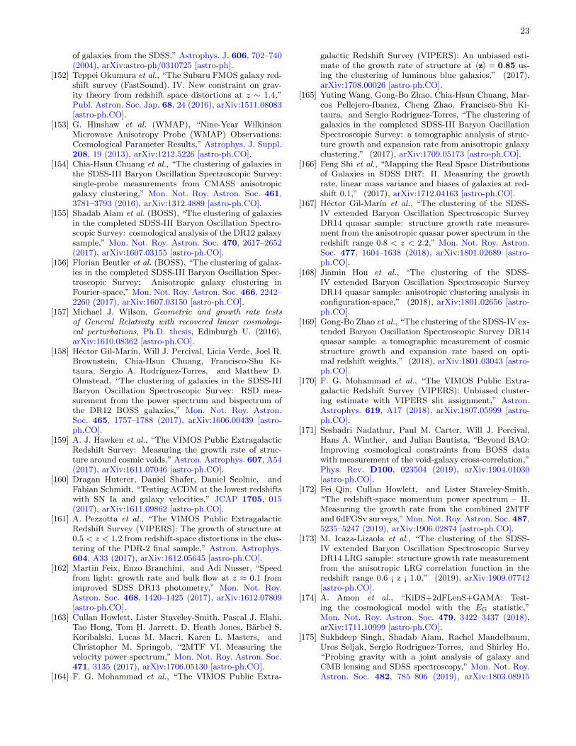
23

of galaxies from the SDSS,” Astrophys. J. 606, 702–740(2004), arXiv:astro-ph/0310725 [astro-ph].

[152] Teppei Okumura et al., “The Subaru FMOS galaxy red-shift survey (FastSound). IV. New constraint on grav-ity theory from redshift space distortions at z ∼ 1.4,”Publ. Astron. Soc. Jap. 68, 24 (2016), arXiv:1511.08083[astro-ph.CO].

[153] G. Hinshaw et al. (WMAP), “Nine-Year WilkinsonMicrowave Anisotropy Probe (WMAP) Observations:Cosmological Parameter Results,” Astrophys. J. Suppl.208, 19 (2013), arXiv:1212.5226 [astro-ph.CO].

[154] Chia-Hsun Chuang et al., “The clustering of galaxies inthe SDSS-III Baryon Oscillation Spectroscopic Survey:single-probe measurements from CMASS anisotropicgalaxy clustering,” Mon. Not. Roy. Astron. Soc. 461,3781–3793 (2016), arXiv:1312.4889 [astro-ph.CO].

[155] Shadab Alam et al. (BOSS), “The clustering of galaxiesin the completed SDSS-III Baryon Oscillation Spectro-scopic Survey: cosmological analysis of the DR12 galaxysample,” Mon. Not. Roy. Astron. Soc. 470, 2617–2652(2017), arXiv:1607.03155 [astro-ph.CO].

[156] Florian Beutler et al. (BOSS), “The clustering of galax-ies in the completed SDSS-III Baryon Oscillation Spec-troscopic Survey: Anisotropic galaxy clustering inFourier-space,” Mon. Not. Roy. Astron. Soc. 466, 2242–2260 (2017), arXiv:1607.03150 [astro-ph.CO].

[157] Michael J. Wilson, Geometric and growth rate testsof General Relativity with recovered linear cosmologi-cal perturbations, Ph.D. thesis, Edinburgh U. (2016),arXiv:1610.08362 [astro-ph.CO].

[158] Hector Gil-Marın, Will J. Percival, Licia Verde, Joel R.Brownstein, Chia-Hsun Chuang, Francisco-Shu Ki-taura, Sergio A. Rodrıguez-Torres, and Matthew D.Olmstead, “The clustering of galaxies in the SDSS-IIIBaryon Oscillation Spectroscopic Survey: RSD mea-surement from the power spectrum and bispectrum ofthe DR12 BOSS galaxies,” Mon. Not. Roy. Astron.Soc. 465, 1757–1788 (2017), arXiv:1606.00439 [astro-ph.CO].

[159] A. J. Hawken et al., “The VIMOS Public ExtragalacticRedshift Survey: Measuring the growth rate of struc-ture around cosmic voids,” Astron. Astrophys. 607, A54(2017), arXiv:1611.07046 [astro-ph.CO].

[160] Dragan Huterer, Daniel Shafer, Daniel Scolnic, andFabian Schmidt, “Testing ΛCDM at the lowest redshiftswith SN Ia and galaxy velocities,” JCAP 1705, 015(2017), arXiv:1611.09862 [astro-ph.CO].

[161] A. Pezzotta et al., “The VIMOS Public ExtragalacticRedshift Survey (VIPERS): The growth of structure at0.5 < z < 1.2 from redshift-space distortions in the clus-tering of the PDR-2 final sample,” Astron. Astrophys.604, A33 (2017), arXiv:1612.05645 [astro-ph.CO].

[162] Martin Feix, Enzo Branchini, and Adi Nusser, “Speedfrom light: growth rate and bulk flow at z ≈ 0.1 fromimproved SDSS DR13 photometry,” Mon. Not. Roy.Astron. Soc. 468, 1420–1425 (2017), arXiv:1612.07809[astro-ph.CO].

[163] Cullan Howlett, Lister Staveley-Smith, Pascal J. Elahi,Tao Hong, Tom H. Jarrett, D. Heath Jones, Barbel S.Koribalski, Lucas M. Macri, Karen L. Masters, andChristopher M. Springob, “2MTF VI. Measuring thevelocity power spectrum,” Mon. Not. Roy. Astron. Soc.471, 3135 (2017), arXiv:1706.05130 [astro-ph.CO].

[164] F. G. Mohammad et al., “The VIMOS Public Extra-

galactic Redshift Survey (VIPERS): An unbiased esti-mate of the growth rate of structure at 〈z〉 = 0.85 us-ing the clustering of luminous blue galaxies,” (2017),arXiv:1708.00026 [astro-ph.CO].

[165] Yuting Wang, Gong-Bo Zhao, Chia-Hsun Chuang, Mar-cos Pellejero-Ibanez, Cheng Zhao, Francisco-Shu Ki-taura, and Sergio Rodriguez-Torres, “The clustering ofgalaxies in the completed SDSS-III Baryon OscillationSpectroscopic Survey: a tomographic analysis of struc-ture growth and expansion rate from anisotropic galaxyclustering,” (2017), arXiv:1709.05173 [astro-ph.CO].

[166] Feng Shi et al., “Mapping the Real Space Distributionsof Galaxies in SDSS DR7: II. Measuring the growthrate, linear mass variance and biases of galaxies at red-shift 0.1,” (2017), arXiv:1712.04163 [astro-ph.CO].

[167] Hector Gil-Marın et al., “The clustering of the SDSS-IV extended Baryon Oscillation Spectroscopic SurveyDR14 quasar sample: structure growth rate measure-ment from the anisotropic quasar power spectrum in theredshift range 0.8 < z < 2.2,” Mon. Not. Roy. Astron.Soc. 477, 1604–1638 (2018), arXiv:1801.02689 [astro-ph.CO].

[168] Jiamin Hou et al., “The clustering of the SDSS-IV extended Baryon Oscillation Spectroscopic SurveyDR14 quasar sample: anisotropic clustering analysis inconfiguration-space,” (2018), arXiv:1801.02656 [astro-ph.CO].

[169] Gong-Bo Zhao et al., “The clustering of the SDSS-IV ex-tended Baryon Oscillation Spectroscopic Survey DR14quasar sample: a tomographic measurement of cosmicstructure growth and expansion rate based on opti-mal redshift weights,” (2018), arXiv:1801.03043 [astro-ph.CO].

[170] F. G. Mohammad et al., “The VIMOS Public Extra-galactic Redshift Survey (VIPERS): Unbiased cluster-ing estimate with VIPERS slit assignment,” Astron.Astrophys. 619, A17 (2018), arXiv:1807.05999 [astro-ph.CO].

[171] Seshadri Nadathur, Paul M. Carter, Will J. Percival,Hans A. Winther, and Julian Bautista, “Beyond BAO:Improving cosmological constraints from BOSS datawith measurement of the void-galaxy cross-correlation,”Phys. Rev. D100, 023504 (2019), arXiv:1904.01030[astro-ph.CO].

[172] Fei Qin, Cullan Howlett, and Lister Staveley-Smith,“The redshift-space momentum power spectrum – II.Measuring the growth rate from the combined 2MTFand 6dFGSv surveys,” Mon. Not. Roy. Astron. Soc. 487,5235–5247 (2019), arXiv:1906.02874 [astro-ph.CO].

[173] M. Icaza-Lizaola et al., “The clustering of the SDSS-IV extended Baryon Oscillation Spectroscopic SurveyDR14 LRG sample: structure growth rate measurementfrom the anisotropic LRG correlation function in theredshift range 0.6 ¡ z ¡ 1.0,” (2019), arXiv:1909.07742[astro-ph.CO].

[174] A. Amon et al., “KiDS+2dFLenS+GAMA: Test-ing the cosmological model with the EG statistic,”Mon. Not. Roy. Astron. Soc. 479, 3422–3437 (2018),arXiv:1711.10999 [astro-ph.CO].

[175] Sukhdeep Singh, Shadab Alam, Rachel Mandelbaum,Uros Seljak, Sergio Rodriguez-Torres, and Shirley Ho,“Probing gravity with a joint analysis of galaxy andCMB lensing and SDSS spectroscopy,” Mon. Not. Roy.Astron. Soc. 482, 785–806 (2019), arXiv:1803.08915

24

[astro-ph.CO].[176] Chris Blake et al., “RCSLenS: Testing gravitational

physics through the cross-correlation of weak lensingand large-scale structure,” Mon. Not. Roy. Astron.Soc. 456, 2806–2828 (2016), arXiv:1507.03086 [astro-ph.CO].

[177] Shadab Alam, Hironao Miyatake, Surhud More, ShirleyHo, and Rachel Mandelbaum, “Testing gravity on large

scales by combining weak lensing with galaxy clusteringusing CFHTLenS and BOSS CMASS,” Mon. Not. Roy.Astron. Soc. 465, 4853–4865 (2017), arXiv:1610.09410[astro-ph.CO].

[178] E. Jullo et al., “Testing gravity with galaxy-galaxy lens-ing and redshift-space distortions using CFHT-Stripe82, CFHTLenS and BOSS CMASS datasets,” Astron.Astrophys. 627, A137 (2019), arXiv:1903.07160 [astro-ph.CO].