Lecture Stat 461-561Wald, Rao and Likelihood Ratio Tests

AD

February 2008

AD () February 2008 1 / 30

Introduction

Wald test

Rao test

Likelihood ratio test

AD () February 2008 2 / 30

Introduction

We want to test H0 : θ = θ0 against H1 : θ 6= θ0 using thelog-likelihood function.

We denote l (θ) the loglikelihood and bθn the consistent root of thelikelihood equation.

Intuitively, the farther bθn is from θ0, the stronger the evidence againstthe null hypothesis.

How far is �far enough�?

AD () February 2008 3 / 30

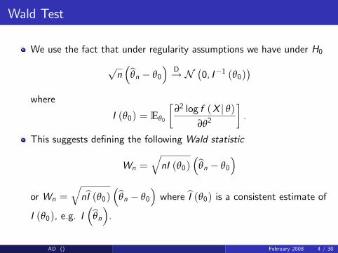
Wald Test

We use the fact that under regularity assumptions we have under H0

pn�bθn � θ0

�D! N

�0, I�1 (θ0)

�where

I (θ0) = Eθ0

�∂2 log f (X j θ)

∂θ2

�.

This suggests de�ning the following Wald statistic

Wn =qnI (θ0)

�bθn � θ0�

or Wn =qnbI (θ0) �bθn � θ0

�where bI (θ0) is a consistent estimate of

I (θ0), e.g. I�bθn�.

AD () February 2008 4 / 30

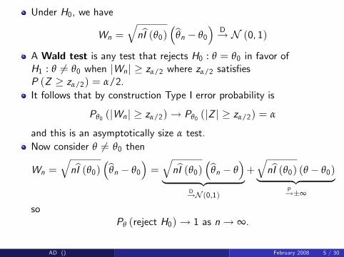
Under H0, we have

Wn =qnbI (θ0) �bθn � θ0

�D! N (0, 1)

A Wald test is any test that rejects H0 : θ = θ0 in favor ofH1 : θ 6= θ0 when jWn j � zα/2 where zα/2 satis�esP (Z � zα/2) = α/2.It follows that by construction Type I error probability is

Pθ0 (jWn j � zα/2)! Pθ0 (jZ j � zα/2) = α

and this is an asymptotically size α test.Now consider θ 6= θ0 then

Wn =qnbI (θ0) �bθn � θ0

�=qnbI (θ0) �bθn � θ

�| {z }

D!N (0,1)

+qnbI (θ0) (θ � θ0)| {z }

P!�∞

soPθ (reject H0)! 1 as n! ∞.

AD () February 2008 5 / 30

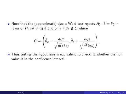
Note that the (approximate) size α Wald test rejects H0 : θ = θ0 infavor of H1 : θ 6= θ0 if and only if θ0 /2 C where

C =

0@bθn � zα/2qnbI (θ0) ,bθn +

zα/2qnbI (θ0)

1A .Thus testing the hypothesis is equivalent to checking whether the nullvalue is in the con�dence interval.

AD () February 2008 6 / 30

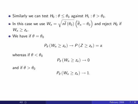
Similarly we can test H0 : θ � θ0 against H1 : θ > θ0.

In this case we use Wn =qnbI (θ0) �bθn � θ0

�and reject H0 if

Wn � zα.

We have if θ = θ0

Pθ (Wn � zα)! P (Z � zα) = α

whereas if θ < θ0Pθ (Wn � zα)! 0

and if θ > θ0Pθ (Wn � zα)! 1.

AD () February 2008 7 / 30

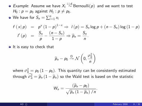
Example: Assume we have Xii.i.d.� Bernoulli(p) and we want to test

H0 : p = p0 against H1 : p 6= p0.We have for Sn = ∑n

i=1 xi

f (x j p) = px (1� p)1�x ) l (p) = Sn log p + (n� Sn) log (1� p)

l 0 (p) =Snp� (n� Sn)

1� p ) bpn = Snn.

It is easy to check that

bpn � p0 D! N�0,

σ20n

�where σ20 = p0 (1� p0). This quantity can be consistently estimatedthrough cσ2n = bpn (1� bpn) so the Wald test is based on the statistic

Wn =(bpn � p0)pbpn (1� bpn) /n

.

AD () February 2008 8 / 30

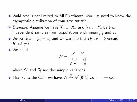
Wald test is not limited to MLE estimate, you just need to know theasymptotic distribution of your test satistic.

Example: Assume we have X1, ...,Xm and Y1, ...,Yn be twoindependent samples from populations with mean µ1 and v .

We write δ = µ1 � µ2 and we want to test H0 : δ = 0 versusH1 : δ 6= 0.We build

W =X � YqS 21m +

S 22m

where S21 and S22 are the sample variances.

Thanks to the CLT, we have WD! N (0, 1) as m, n! ∞.

AD () February 2008 9 / 30

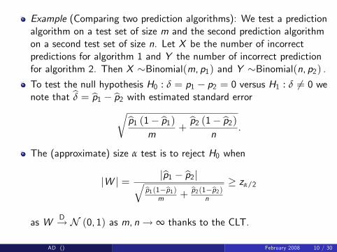
Example (Comparing two prediction algorithms): We test a predictionalgorithm on a test set of size m and the second prediction algorithmon a second test set of size n. Let X be the number of incorrectpredictions for algorithm 1 and Y the number of incorrect predictionfor algorithm 2. Then X �Binomial(m, p1) and Y �Binomial(n, p2) .To test the null hypothesis H0 : δ = p1 � p2 = 0 versus H1 : δ 6= 0 wenote that bδ = bp1 � bp2 with estimated standard errorrbp1 (1� bp1)

m+bp2 (1� bp2)

n.

The (approximate) size α test is to reject H0 when

jW j = jbp1 � bp2jq bp1(1�bp1)m + bp2(1�bp2)

n

� zα/2

as WD! N (0, 1) as m, n! ∞ thanks to the CLT.

AD () February 2008 10 / 30

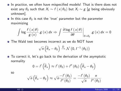
In practice, we often have mispeci�ed models! That is there does notexist any θ0 such that Xi � f (x j θ0) but Xi � g [g being obviouslyunknown].In this case θ0 is not the �true�parameter but the parametermaximizingZ

logf (x j θ)g (x)

.g (x) dx )Z

∂ log f (x j θ)∂θ

����θ=θ0

.g (x) dx = 0

The Wald test becomes incorrect as we do NOT havepn�bθn � θ0

�D! N

�0, I�1 (θ0)

�To correct it, let�s go back to the derivation of the asymptoticnormality

0 = l 0�bθn� � l 0 (θ0) + l 00 (θ0) �bθn � θ0

�so

pn�bθn � θ0

��pn�l 0 (θ0)l 00 (θ0)

=�l 0 (θ0)p

nn

l 00 (θ0)

AD () February 2008 11 / 30

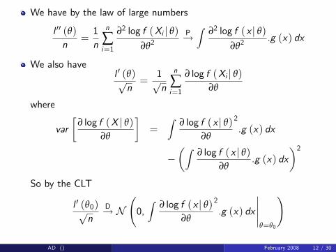
We have by the law of large numbers

l 00 (θ)n

=1n

n

∑i=1

∂2 log f (Xi j θ)∂θ2

P!Z

∂2 log f (x j θ)∂θ2

.g (x) dx

We also havel 0 (θ)pn=

1pn

n

∑i=1

∂ log f (Xi j θ)∂θ

where

var�

∂ log f (X j θ)∂θ

�=

Z∂ log f (x j θ)

∂θ

2

.g (x) dx

��Z

∂ log f (x j θ)∂θ

.g (x) dx�2

So by the CLT

l 0 (θ0)pn

D! N 0,Z

∂ log f (x j θ)∂θ

2

.g (x) dx

�����θ=θ0

!

AD () February 2008 12 / 30

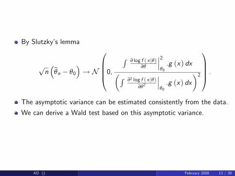
By Slutzky�s lemma

pn�bθn � θ0

�! N

0BBB@0,R ∂ log f ( x jθ)

∂θ

���2θ0.g (x) dx�R ∂2 log f ( x jθ)

∂θ2

���θ0.g (x) dx

�21CCCA .

The asymptotic variance can be estimated consistently from the data.

We can derive a Wald test based on this asymptotic variance.

AD () February 2008 13 / 30

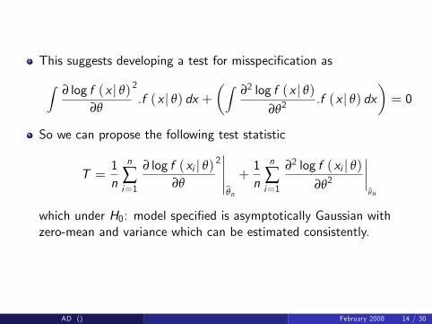
This suggests developing a test for misspeci�cation as

Z∂ log f (x j θ)

∂θ

2

.f (x j θ) dx +�Z

∂2 log f (x j θ)∂θ2

.f (x j θ) dx�= 0

So we can propose the following test statistic

T =1n

n

∑i=1

∂ log f (xi j θ)∂θ

2�����bθn +

1n

n

∑i=1

∂2 log f (xi j θ)∂θ2

����bθnwhich under H0: model speci�ed is asymptotically Gaussian withzero-mean and variance which can be estimated consistently.

AD () February 2008 14 / 30

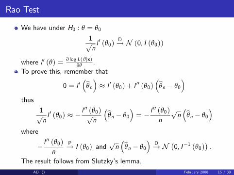
Rao Test

We have under H0 : θ = θ0

1pnl 0 (θ0)

D! N (0, I (θ0))

where l 0 (θ) = ∂ log L( θjx)∂θ .

To prove this, remember that

0 = l 0�bθn� � l 0 (θ0) + l 00 (θ0) �bθn � θ0

�thus

1pnl 0 (θ0) � �

l 00 (θ0)pn

�bθn � θ0�= � l

00 (θ0)

n

pn�bθn � θ0

�where

� l00 (θ0)

nP! I (θ0) and

pn�bθn � θ0

�D! N

�0, I�1 (θ0)

�.

The result follows from Slutzky�s lemma.AD () February 2008 15 / 30

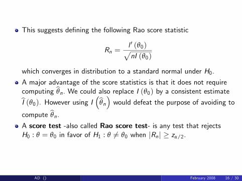
This suggests de�ning the following Rao score statistic

Rn =l 0 (θ0)pnI (θ0)

which converges in distribution to a standard normal under H0.

A major advantage of the score statistics is that it does not requirecomputing bθn. We could also replace I (θ0) by a consistent estimatebI (θ0). However using I �bθn� would defeat the purpose of avoiding tocompute bθn.A score test -also called Rao score test- is any test that rejectsH0 : θ = θ0 in favor of H1 : θ 6= θ0 when jRn j � zα/2.

AD () February 2008 16 / 30

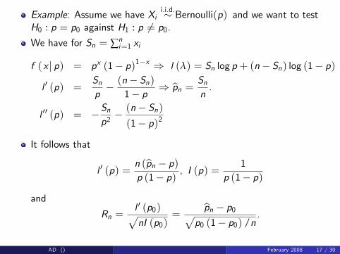
Example: Assume we have Xii.i.d.� Bernoulli(p) and we want to test

H0 : p = p0 against H1 : p 6= p0.We have for Sn = ∑n

i=1 xi

f (x j p) = px (1� p)1�x ) l (λ) = Sn log p + (n� Sn) log (1� p)

l 0 (p) =Snp� (n� Sn)

1� p ) bpn = Snn.

l 00 (p) = �Snp2� (n� Sn)(1� p)2

It follows that

l 0 (p) =n (bpn � p)p (1� p) , I (p) =

1p (1� p)

and

Rn =l 0 (p0)pnI (p0)

=bpn � p0p

p0 (1� p0) /n.

AD () February 2008 17 / 30

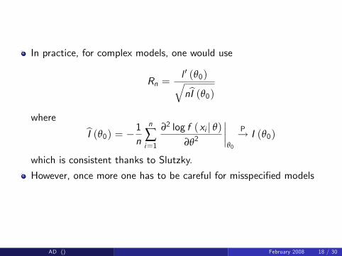
In practice, for complex models, one would use

Rn =l 0 (θ0)qnbI (θ0)

where bI (θ0) = �1n n

∑i=1

∂2 log f (xi j θ)∂θ2

����θ0

P! I (θ0)

which is consistent thanks to Slutzky.

However, once more one has to be careful for misspeci�ed models

AD () February 2008 18 / 30

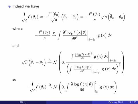
Indeed we have

1pnl 0 (θ0) � �

l 00 (θ0)pn

�bθn � θ0�= � l

00 (θ0)

n

pn�bθn � θ0

�where

� l00 (θ0)

nP!Z

∂2 log f (x j θ)∂θ2

����θ=θ0

.g (x) dx

and

pn�bθn � θ0

�D! N

0BBB@0,R ∂ log f ( x jθ)

∂θ

2.g (x) dx

����θ=θ0�R ∂2 log f ( x jθ)

∂θ2

���θ=θ0

.g (x) dx�21CCCA

so1pnl 0 (θ0)

D! N 0,Z

∂ log f (x j θ)∂θ

����2θ0

.g (x) dx

!

AD () February 2008 19 / 30

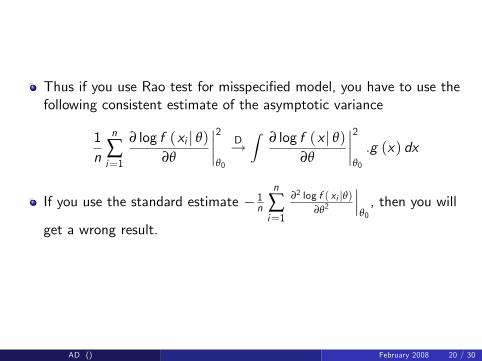
Thus if you use Rao test for misspeci�ed model, you have to use thefollowing consistent estimate of the asymptotic variance

1n

n

∑i=1

∂ log f (xi j θ)∂θ

����2θ0

D!Z

∂ log f (x j θ)∂θ

����2θ0

.g (x) dx

If you use the standard estimate � 1n

n

∑i=1

∂2 log f ( xi jθ)∂θ2

���θ0, then you will

get a wrong result.

AD () February 2008 20 / 30

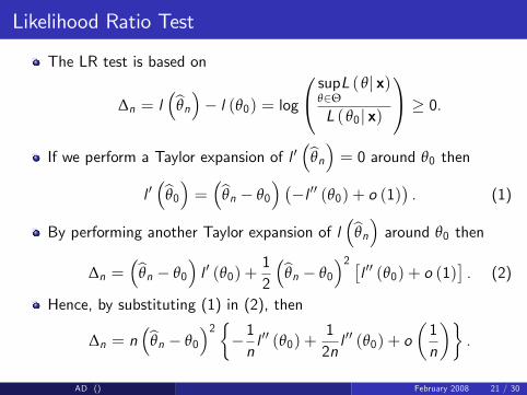
Likelihood Ratio Test

The LR test is based on

∆n = l�bθn�� l (θ0) = log

0@ supθ2ΘL ( θj x)

L ( θ0j x)

1A � 0.

If we perform a Taylor expansion of l 0�bθn� = 0 around θ0 then

l 0�bθ0� = �bθn � θ0

� ��l 00 (θ0) + o (1)

�. (1)

By performing another Taylor expansion of l�bθn� around θ0 then

∆n =�bθn � θ0

�l 0 (θ0) +

12

�bθn � θ0�2 �

l 00 (θ0) + o (1)�. (2)

Hence, by substituting (1) in (2), then

∆n = n�bθn � θ0

�2 ��1nl 00 (θ0) +

12nl 00 (θ0) + o

�1n

��.

AD () February 2008 21 / 30

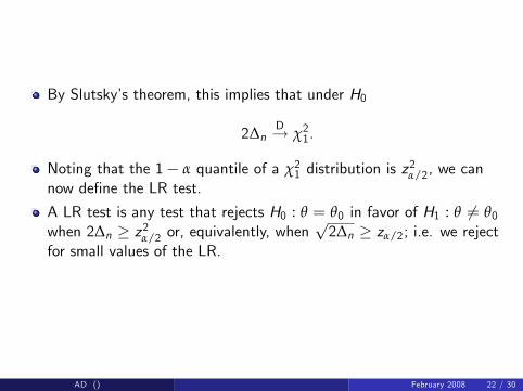
By Slutsky�s theorem, this implies that under H0

2∆nD! χ21.

Noting that the 1� α quantile of a χ21 distribution is z2α/2, we can

now de�ne the LR test.

A LR test is any test that rejects H0 : θ = θ0 in favor of H1 : θ 6= θ0when 2∆n � z2α/2 or, equivalently, when

p2∆n � zα/2; i.e. we reject

for small values of the LR.

AD () February 2008 22 / 30

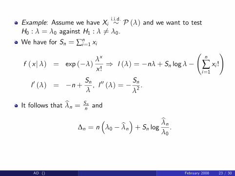
Example: Assume we have Xii.i.d.� P (λ) and we want to test

H0 : λ = λ0 against H1 : λ 6= λ0.

We have for Sn = ∑ni=1 xi

f (x j λ) = exp (�λ)λx

x !) l (λ) = �nλ+ Sn log λ�

n

∑i=1xi !

!

l 0 (λ) = �n+ Snλ, l 00 (λ) = �Sn

λ2.

It follows that bλn = Snn and

∆n = n�

λ0 � bλn�+ Sn log bλnλ0.

AD () February 2008 23 / 30

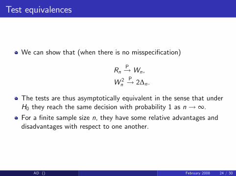
Test equivalences

We can show that (when there is no misspeci�cation)

RnP! Wn,

W 2n

P! 2∆n.

The tests are thus asymptotically equivalent in the sense that underH0 they reach the same decision with probability 1 as n! ∞.For a �nite sample size n, they have some relative advantages anddisadvantages with respect to one another.

AD () February 2008 24 / 30

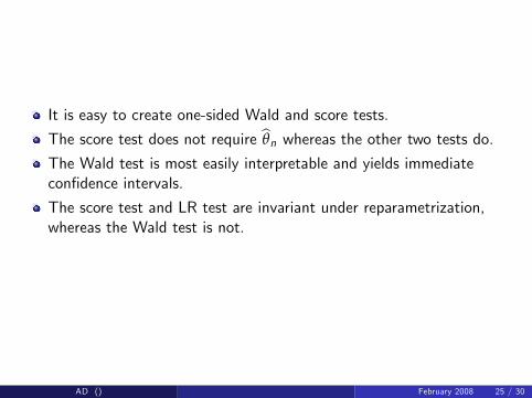
It is easy to create one-sided Wald and score tests.

The score test does not require bθn whereas the other two tests do.The Wald test is most easily interpretable and yields immediatecon�dence intervals.

The score test and LR test are invariant under reparametrization,whereas the Wald test is not.

AD () February 2008 25 / 30

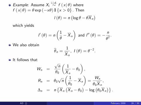
Example: Assume Xii.i.d.� f (x j θ) where

f (x j θ) = θ exp (�xθ) I fx > 0g . Thenl (θ) = n

�log θ � θX n

�which yields

l 0 (θ) = n�1θ� X n

�and l 00 (θ) = � n

θ2.

We also obtain bθn = 1

X n, I (θ) = θ�2.

It follows that

Wn =

pn

θ0

�1

X n� θ0

�,

Rn = θ0pn�1θ0� X n

�=

Wn

θ0X n,

∆n = n�X n�X n � θ0

�� log

�θ0X n

�.

AD () February 2008 26 / 30

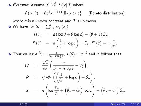
Example: Assume Xii.i.d.� f (x j θ) where

f (x j θ) = θcθx�(θ+1)I fx > cg (Pareto distribution)

where c is a known constant and θ is unknown.We have for Sn = ∑n

i=1 log (xi )

l (θ) = n (log θ + θ log c)� (θ + 1) Sn,

l 0 (θ) = n�1θ+ log c

�� Sn, l 00 (θ) = �

n

θ2.

Thus we have bθn = nSn�n log c , I (θ) = θ�2 and it follows that

Wn =

pn

θ0

�n

Sn � n log c� θ0

�,

Rn =pnθ0

��1θ0+ log c

�� Sn

�,

∆n = n

logbθnθ0+�bθn � θ0

�log c

!��bθn � θ0

�Sn.

AD () February 2008 27 / 30

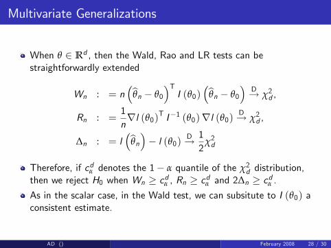
Multivariate Generalizations

When θ 2 Rd , then the Wald, Rao and LR tests can bestraightforwardly extended

Wn : = n�bθn � θ0

�TI (θ0)

�bθn � θ0�

D! χ2d ,

Rn : =1nrl (θ0)T I�1 (θ0)rl (θ0) D! χ2d ,

∆n : = l�bθn�� l (θ0) D! 1

2χ2d

Therefore, if cdα denotes the 1� α quantile of the χ2d distribution,then we reject H0 when Wn � cdα , Rn � cdα and 2∆n � cdα .As in the scalar case, in the Wald test, we can subsitute to I (θ0) aconsistent estimate.

AD () February 2008 28 / 30

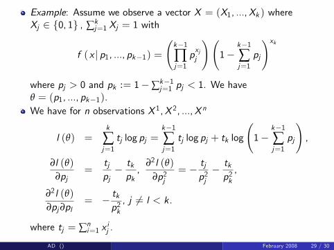
Example: Assume we observe a vector X = (X1, ...,Xk ) whereXj 2 f0, 1g , ∑k

j=1 Xj = 1 with

f (x j p1, ..., pk�1) = k�1∏j=1

pxjj

! 1�

k�1∑j=1

pj

!xkwhere pj > 0 and pk := 1�∑k�1

j=1 pj < 1. We haveθ = (p1, ..., pk�1).We have for n observations X 1,X 2, ...,X n

l (θ) =k

∑j=1tj log pj =

k�1∑j=1

tj log pj + tk log

1�

k�1∑j=1

pj

!,

∂l (θ)∂pj

=tjpj� tkpk,

∂2l (θ)∂p2j

= � tjp2j� tkp2k,

∂2l (θ)∂pj∂pl

= � tkp2k, j 6= l < k.

where tj = ∑ni=1 x

ij .

AD () February 2008 29 / 30

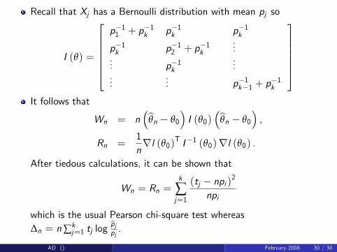
Recall that Xj has a Bernoulli distribution with mean pj so

I (θ) =

2666664p�11 + p�1k p�1k p�1kp�1k p�12 + p�1k

...... p�1k

......

... p�1k�1 + p�1k

3777775It follows that

Wn = n�bθn � θ0

�I (θ0)

�bθn � θ0�,

Rn =1nrl (θ0)T I�1 (θ0)rl (θ0) .

After tiedous calculations, it can be shown that

Wn = Rn =k

∑j=1

(tj � npi )2

npi

which is the usual Pearson chi-square test whereas∆n = n∑k

j=1 tj logbpjpj.

AD () February 2008 30 / 30