Extremal and Kcsc resolutions - Vanderbilt Universitykahlergeometry/Arezzo_Talk.pdf · for...
36
Extremal and Kcsc resolutions Vanderbilt University, Nashville TN May 21, 2015
Transcript of Extremal and Kcsc resolutions - Vanderbilt Universitykahlergeometry/Arezzo_Talk.pdf · for...
Extremal and Kcsc resolutions
Vanderbilt University, Nashville TN
May 21, 2015
Background The linear problem Results
Joint work with R. Lena and L. Mazzieri. Basic problem:
Given a compact orbifold (M, g , ω) of complex dimension m with anextremal metric g , isolated quotient singularities and orbifold groupsΓj / U(m), whose local singularities Cm/Γj admits a scalar flat ALE
Kahler resolutions(XΓj , hj , ηj
), is there an extremal resolution
(M, g , ω
)which replaces a neighbourhood of each singular point pj with (a largepiece of) the resolution XΓj ?
If g is Kahler constant scalar curvature (Kcsc from now on), when is thesolution of the above problem Kcsc as well?
Background The linear problem Results
Remark
If we have the models(XΓj , hj , ηj
), i = 1, . . . , S we can construct the
manifold
M := M tx1,ε XΓ1 tx2,ε · · · txS ,ε XΓS
where the operation txj ,ε is performed removing a small ball of radius rεaround xj on M and a removing a large ball or radius Rε on XΓj settingRε = rε
ε.
This can be interpreted as a “jump of complex structure” at ε = 0 (infact a jump of the manifold itself!) but then the complex structure of Mdoes not depend on ε for ε 6= 0.
One could ask a similar question with more delicate models, where thecomplex structure is only asymptotic to the one of M (e.g. “smoothings”a la Spotti-Biquard-Rollin and/or Jeff and Ha-Jo’s talks).

Background The linear problem Results
Foundational/Inspirational results in the smooth case:
Since we think of our problem as so closely related to the deformation problemfor extremal/Kcsc moving the Kahler class and keeping J fixed, let’s go back tothe smooth case to get some feeling:
LeBrun-Simanca:
Theorem
The extremal cone is open in the Kahler cone.
Calabi:
Theorem
Let g be extremal. Then g has constant scalar curvature if and only ifFut(·, g) = 0.
Rem:
F (X , g) =
∫M
X (hg )dVolg ,S(g) − 1
Vol
∫M
S(g)dVolg = ∆ghg
and X is a holomorphic vector field.
Background The linear problem Results
Futaki invariant:
First observation: if there are no holomorphic vector fields, the deformationproblem is unobstructed also in Kcsc case.In general, the solution to the extremal problem plus the knowledge of theFutaki invariant in the deformed classes gives the solution also to the Kcscproblem. In the case we are blowing up points, the expansion in ε of the Futakiinvariant has been computed by Stoppa, Odaka, Della Vedova-Zuddas andSzekelyhidi up to second order. For resolution of singularities we do not know.On top of this it is important to see the obstruction inside the PDE as for theKE problem in a non-definite first Chern class manifold.
Background The linear problem Results
The linearized equation
For a smooth real function f ∈ C∞(M) such that ω + i∂∂f > 0, we set
ωf = ω + i∂∂f ,
Since we want to understand the behavior of the scalar curvature underdeformations of this type, it is convenient to consider the following differentialoperator
Sω(·) : C∞(M) −→ C∞(M) , f 7−→ Sω(f ) := sω+i∂∂f ,
Sω(f ) = sω −1
2Lωf +
1
2Nω(f ) ,
where the linearized scalar curvature operator Lω is given by
Lωf = ∆2ωf + 4 〈 ρω | i∂∂f 〉 .

Background The linear problem Results
The subspace of ker(L) given by the elements with zero mean is in one toone correspondence with the space of holomorphic vector fields whichvanish somewhere in M.
From now on we set
ker (Lω) = spanR {1, ϕ1, . . . , ϕd} .
Background The linear problem Results
The subspace of ker(L) given by the elements with zero mean is in one toone correspondence with the space of holomorphic vector fields whichvanish somewhere in M.
From now on we set
ker (Lω) = spanR {1, ϕ1, . . . , ϕd} .
Background The linear problem Results
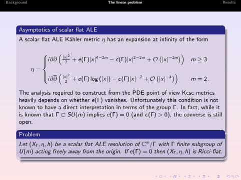
Asymptotics of scalar flat ALE
A scalar flat ALE Kahler metric η has an expansion at infinity of the form
η =
i∂∂
(|x|2
2+ e(Γ)|x |4−2m − c(Γ)|x |2−2m +O
(|x |−2m
))m ≥ 3
i∂∂(|x|2
2+ e(Γ) log (|x |)− c(Γ)|x |−2 +O
(|x |−4
))m = 2 .
The analysis required to construct from the PDE point of view Kcsc metricsheavily depends on whether e(Γ) vanishes. Unfortunately this condition is notknown to have a direct interpretation in terms of the group Γ. In fact, while itis known that Γ ⊂ SU(m) implies e(Γ) = 0 (and c(Γ) > 0), the converse is stillopen.
Problem
Let (XΓ, η, h) be a scalar flat ALE resolution of Cm/Γ with Γ finite subgroup ofU(m) acting freely away from the origin. If e(Γ) = 0 then (XΓ, η, h) is Ricci-flat.
Background The linear problem Results
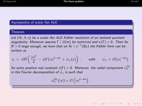
Asymptotics of scalar flat ALE
Theorem
Let (XΓ, h, η) be a scalar flat ALE Kahler resolution of an isolated quotientsingularitiy. Moreover assume Γ / U(m) be nontrivial and e (Γ) = 0. Then forR > 0 large enough, we have that on XΓ \ π−1(BR) the Kahler form can bewritten as
η = i∂∂
(|x |2
2− c(Γ) |x |2−2m + ψη (x)
), with ψη = O(|x |−2m) ,
for some positive real constant c(Γ) > 0. Moreover, the radial component ψ(0)η
in the Fourier decomposition of ψη is such that
ψ(0)η (|x |) = O
(|x |2−4m
).
Background The linear problem Results
no holom. vector fields
A-Pacard:
Theorem
If there are no holomorphic vector fields, the Kcsc problem has always positivesolution.
When holomorphic vector fields exist, then the solution depends strongly on thegroups Γj and the position of the singular points.
Background The linear problem Results
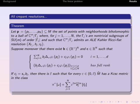
All crepant resolutions...
Theorem
Let p = {p1, . . . , pN} ⊆ M the set of points with neighborhoods biholomorphicto a ball of Cm/Γj where, for j = 1, . . . ,N, the Γj ’s are nontrivial subgroups ofSU(m) of order |Γj | and such that Cm/Γj admits an ALE Kahler Ricci-flatresolution
(XΓj , hj , ηj
).
Suppose moreover that there exist b ∈ (R+)N and c ∈ RN such that∑N
j=1 bj∆ωϕi (pj) + cjϕi (pj) = 0 i = 1, . . . , d
(bj∆ωϕi (pj) + cjϕi (pj))1≤i≤d1≤j≤N
has full rank
If cj = sωbj , then there is ε such that for every ε ∈ (0, ε) M has a Kcsc metricin the class
π∗ [ω] +N∑j=1
ε2mb2mj [ηj ]
Background The linear problem Results
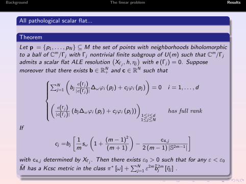
All pathological scalar flat...
Theorem
Let p = {p1, . . . , pN} ⊆ M the set of points with neighborhoods biholomorphicto a ball of Cm/Γj with Γj nontrivial finite subgroup of U(m) such that Cm/Γj
admits a scalar flat ALE resolution(XΓj , h, ηj
)with e (Γj) = 0. Suppose
moreover that there exists b ∈ RN+ and c ∈ RN such that
∑Nj=1
(bj
c(Γj)|c(Γj)|
∆ωϕi (pj) + cjϕi (pj)
)= 0 i = 1, . . . , d
(c(Γj)|c(Γj)|
(bj∆ωϕi (pj) + cjϕi (pj))
)1≤i≤d1≤j≤N
has full rank
If
cj =bj
[1
msω
(1 +
(m − 1)2
(m + 1)
)− c4,j
2 (m − 1) |S2m−1|
]with c4,j determined by XΓj . Then there exists ε0 > 0 such that for any ε < ε0
M has a Kcsc metric in the class π∗ [ω] +∑N
j=1 ε2mb2m
j [ηj ] .
Background The linear problem Results
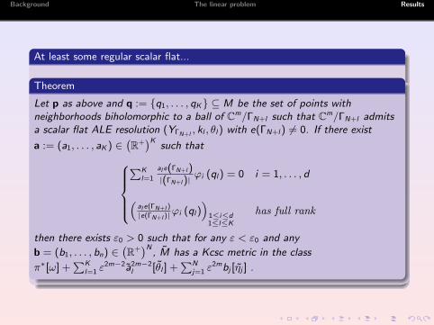
At least some regular scalar flat...
Theorem
Let p as above and q := {q1, . . . , qK} ⊆ M be the set of points withneighborhoods biholomorphic to a ball of Cm/ΓN+l such that Cm/ΓN+l admitsa scalar flat ALE resolution (YΓN+l , kl , θl) with e(ΓN+l) 6= 0. If there exist
a := (a1, . . . , aK ) ∈(R+)K
such that∑K
l=1
al e(ΓN+l)|(ΓN+l)|
ϕi (ql) = 0 i = 1, . . . , d
(al e(ΓN+l )
|e(ΓN+l )|ϕi (ql)
)1≤i≤d1≤l≤K
has full rank
then there exists ε0 > 0 such that for any ε < ε0 and any
b = (b1, . . . , bn) ∈(R+)N
, M has a Kcsc metric in the class
π∗[ω] +∑K
l=1 ε2m−2a2m−2
l [θl ] +∑N
j=1 ε2mbj [ηj ] .
Background The linear problem Results
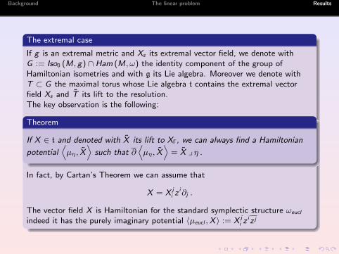
The extremal case
If g is an extremal metric and Xs its extremal vector field, we denote withG := Iso0 (M, g) ∩ Ham (M, ω) the identity component of the group ofHamiltonian isometries and with g its Lie algebra. Moreover we denote withT ⊂ G the maximal torus whose Lie algebra t contains the extremal vectorfield Xs and T its lift to the resolution.The key observation is the following:
Theorem
If X ∈ t and denoted with X its lift to XΓ, we can always find a Hamiltonian
potential⟨µη, X
⟩such that ∂
⟨µη, X
⟩= X y η .
In fact, by Cartan’s Theorem we can assume that
X = X ji z i∂j .
The vector field X is Hamiltonian for the standard symplectic structure ωeucl
indeed it has the purely imaginary potential 〈µeucl ,X 〉 := X ji z iz j

Background The linear problem Results
proof continued...
Denoting with π : XΓ −→ Cm/Γ the canonical surjection we consider ξ the(0, 1)-form on XΓ defined as
ξ := X y [η − π∗ωeucl ]
clearly ξ ∈ L2 (XΓ, h) and moreover ∂ξ = 0. From Joyce we deduce that thefirst L2-cohomology group H1
L2 (XΓ,C) is isomorphic to the first De Rhamcohomology group H1 (XΓ,C) and by simply-connectedness of resolutions wehave that H1 (XΓ,C) = {0}. Moreover by L2-cohomology theory, we find that
ξ = ∂f
with f complex function in L2 (XΓ, h). Using the mapping properties of theLaplace operator It is possible to obtain more informations on f . We have,
indeed, that ξ ∈ C 1,α1−2m
(XΓ, (T ∗XΓ)(1,0)
)by construction and hence a simple
computation yields ∂∗ξ ∈ C 0,α
−2m (XΓ,C).
Background The linear problem Results
proof continued...
Now∆ηf = 2∂
∗ξ
and using the surjectivity of the Laplace operator
∆η : C 2,αδ (XΓ,C) −→ C 0,α
δ−2 (XΓ,C) δ ∈ (3− 2m, 2− 2m)
and the fact that ∆η has no bounded kernel we conclude thatf ∈ C 2,α
δ (XΓ,C) ∩ C∞loc (XΓ) with δ ∈ (3− 2m, 2− 2m). Now we have, byconstruction, that
∂ [π∗ 〈µeucl ,Ξ〉+ f ] = Ξ y η
and henceLη [π∗ 〈µeucl ,Ξ〉+ f ] = 0 .
Since the metric h is scalar flat, Lη is a real operator and consequently boththe real and the imaginary part of π∗ 〈µeucl ,Ξ〉+ f are in the kernel of Lη. Thereal part of π∗ 〈µeucl ,Ξ〉+ f coincides with the real part of f since π∗ 〈µeucl ,Ξ〉is purely imaginary, hence f is bounded and by the wighted analysis on themodel it has to vanish identically.
Background The linear problem Results
The extremal gluing
Theorem
Let (M, g , ω) be a compact extremal orbifold with T -invariant metric g andsingular points {x1, . . . , xS}. Then there exists ε such that for every ε ∈ (0, ε)the resolution
M := M tx1,ε XΓ1 tx2,ε · · · txS ,ε XΓS
has a T -invariant extremal Kahler metric.
Background The linear problem Results
Examples
Example
Consider(P1 × P1, π∗1ωFS + π∗2ωFS
)and let Z2 act in the following way
([x0 : x1], [y0 : y1]) −→ ([x0 : −x1], [y0 : −y1])
It’s immediate to check that this action is in SU(2) with four fixed points
p1 = ([1 : 0], [1 : 0])
p2 = ([1 : 0], [0 : 1])
p3 = ([0 : 1], [1 : 0])
p4 = ([0 : 1], [0 : 1])
The quotient space X2 := P1 × P1/Z2 is a Kahler-Einstein, Fano orbifold andthanks to the embedding into P4
([x0 : x1], [y0 : y1]) 7→ [x20 y 2
0 : x20 y 2
1 : x21 y 2
0 : x21 y 2
1 : x0x1y0y1]
it is isomorphic to the intersection of singular quadrics{z0z3 − z2
4 = 0}∩{
z1z2 − z24 = 0
}
Background The linear problem Results
Examples
Example
Hence it is a limit of Kahler-Einstein surfaces, namely the intersection of twosmooth quadrics. Since it is Kahler-Einstein, so we have to verify that thematrix
Θ (1, sω1) =( sω
2ϕj (pi )
)1≤i≤21≤j≤4
.
has full rank and there exist a positive element in ker Θ (1, sω1). It isimmediate to see that we have
H0(
X2,T(1,0)X2
)= H0
(P1/Z2,T
(1,0)(P1/Z2
))⊕H0
(P1/Z2,T
(1,0)(P1/Z2
)).
MoreoverH0(P1/Z2,T
(1,0)(P1/Z2
))is generated by holomorphic vector fields on P1 that vanish on points[0 : 1], [1 : 0] so
dimC H0(P1/Z2,T
(1,0)(P1/Z2
))= 1
and an explicit generator is the vector field
V = z1∂1 .
Background The linear problem Results
Examples
Example
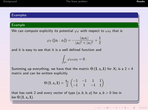
We can compute explicitly its potential ϕV with respect to ωFS that is
ϕV ([z0 : z1]) = − |z0z1||z0|2 + |z1|2
+1
2
and it is easy to see that it is a well defined function and∫P1
ϕVωFS = 0 .
Summing up everything, we have that the matrix Θ (1, sω1) for X2 is a 2× 4matrix and can be written explicitly
Θ (1, sω1) =sω2
(−1 −1 1 1−1 1 −1 1
)that has rank 2 and every vector of type (a, b, b, a) for a, b > 0 lies inker Θ (1, sω1).
Background The linear problem Results
Examples
Example
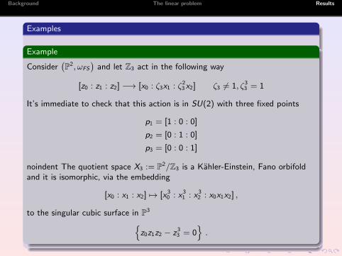
Consider(P2, ωFS
)and let Z3 act in the following way
[z0 : z1 : z2] −→ [x0 : ζ3x1 : ζ23 x2] ζ3 6= 1, ζ3
3 = 1
It’s immediate to check that this action is in SU(2) with three fixed points
p1 = [1 : 0 : 0]
p2 = [0 : 1 : 0]
p3 = [0 : 0 : 1]
noindent The quotient space X3 := P2/Z3 is a Kahler-Einstein, Fano orbifoldand it is isomorphic, via the embedding
[x0 : x1 : x2] 7→ [x30 : x3
1 : x32 : x0x1x2] ,
to the singular cubic surface in P3{z0z1z2 − z3
3 = 0}.
Background The linear problem Results
Examples
Example
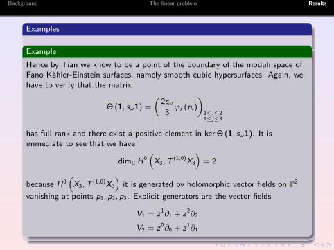
Hence by Tian we know to be a point of the boundary of the moduli space ofFano Kahler-Einstein surfaces, namely smooth cubic hypersurfaces. Again, wehave to verify that the matrix
Θ (1, sω1) =
(2sω
3ϕj (pi )
)1≤i≤21≤j≤3
.
has full rank and there exist a positive element in ker Θ (1, sω1). It isimmediate to see that we have
dimC H0(
X3,T(1,0)X3
)= 2
because H0(
X3,T(1,0)X3
)it is generated by holomorphic vector fields on P2
vanishing at points p1, p2, p3. Explicit generators are the vector fields
V1 = z1∂1 + z2∂2
V2 = z0∂0 + z1∂1
Background The linear problem Results
Examples
Example
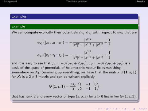
We can compute explicitly their potentials φV1 , φV2 with respect to ωFS that are
φV1 ([z0 : z1 : z2]) = − |z0|2
|z0|2 + |z1|2 + |z2|2 +1
3
φV2 ([z0 : z1 : z2]) = − |z2|2
|z0|2 + |z1|2 + |z2|2 +1
3
and it is easy to see that ϕ1 = −3 (φV1 + 2φV2 ) , ϕ2 = −3 (2φV1 + φV2 ) is abasis of the space of potentials of holomorphic vector fields vanishingsomewhere on X3. Summing up everything, we have that the matrix Θ (1, sω1)for X3 is a 2× 3 matrix and can be written explicitly
Θ (1, sω1) =2sω
3
(1 −1 00 −1 1
)that has rank 2 and every vector of type (a, a, a) for a > 0 lies in ker Θ (1, sω1).
Background The linear problem Results
Examples
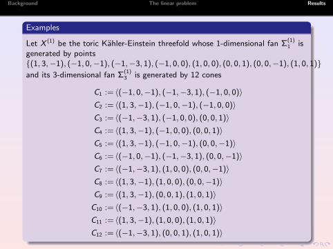
Let X (1) be the toric Kahler-Einstein threefold whose 1-dimensional fan Σ(1)1 is
generated by points{(1, 3,−1), (−1, 0,−1), (−1,−3, 1), (−1, 0, 0), (1, 0, 0), (0, 0, 1), (0, 0,−1), (1, 0, 1)}and its 3-dimensional fan Σ
(1)3 is generated by 12 cones
C1 := 〈(−1, 0,−1), (−1,−3, 1), (−1, 0, 0)〉C2 := 〈(1, 3,−1), (−1, 0,−1), (−1, 0, 0)〉C3 := 〈(−1,−3, 1), (−1, 0, 0), (0, 0, 1)〉C4 := 〈(1, 3,−1), (−1, 0, 0), (0, 0, 1)〉C5 := 〈(1, 3,−1), (−1, 0,−1), (0, 0,−1)〉C6 := 〈(−1, 0,−1), (−1,−3, 1), (0, 0,−1)〉C7 := 〈(−1,−3, 1), (1, 0, 0), (0, 0,−1)〉C8 := 〈(1, 3,−1), (1, 0, 0), (0, 0,−1)〉C9 := 〈(1, 3,−1), (0, 0, 1), (1, 0, 1)〉
C10 := 〈(−1,−3, 1), (1, 0, 0), (1, 0, 1)〉C11 := 〈(1, 3,−1), (1, 0, 0), (1, 0, 1)〉C12 := 〈(−1,−3, 1), (0, 0, 1), (1, 0, 1)〉
Background The linear problem Results
Examples
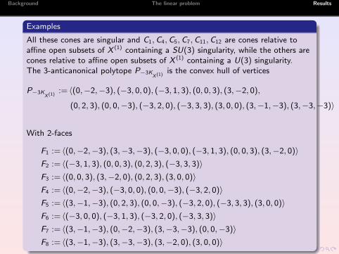
All these cones are singular and C1,C4,C5,C7,C11,C12 are cones relative toaffine open subsets of X (1) containing a SU(3) singularity, while the others arecones relative to affine open subsets of X (1) containing a U(3) singularity.The 3-anticanonical polytope P−3K
X (1)is the convex hull of vertices
P−3KX (1)
:= 〈(0,−2,−3), (−3, 0, 0), (−3, 1, 3), (0, 0, 3), (3,−2, 0),
(0, 2, 3), (0, 0,−3), (−3, 2, 0), (−3, 3, 3), (3, 0, 0), (3,−1,−3), (3,−3,−3)〉
With 2-faces
F1 := 〈(0,−2,−3), (3,−3,−3), (−3, 0, 0), (−3, 1, 3), (0, 0, 3), (3,−2, 0)〉F2 := 〈(−3, 1, 3), (0, 0, 3), (0, 2, 3), (−3, 3, 3)〉F3 := 〈(0, 0, 3), (3,−2, 0), (0, 2, 3), (3, 0, 0)〉F4 := 〈(0,−2,−3), (−3, 0, 0), (0, 0,−3), (−3, 2, 0)〉F5 := 〈(3,−1,−3), (0, 2, 3), (0, 0,−3), (−3, 2, 0), (−3, 3, 3), (3, 0, 0)〉F6 := 〈(−3, 0, 0), (−3, 1, 3), (−3, 2, 0), (−3, 3, 3)〉F7 := 〈(3,−1,−3), (0,−2,−3), (3,−3,−3), (0, 0,−3)〉F8 := 〈(3,−1,−3), (3,−3,−3), (3,−2, 0), (3, 0, 0)〉
Background The linear problem Results
Examples
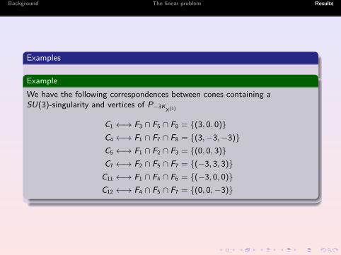
Example
We have the following correspondences between cones containing aSU(3)-singularity and vertices of P−3K
X (1)
C1 ←→ F3 ∩ F5 ∩ F8 = {(3, 0, 0)}C4 ←→ F1 ∩ F7 ∩ F8 = {(3,−3,−3)}C5 ←→ F1 ∩ F2 ∩ F3 = {(0, 0, 3)}C7 ←→ F2 ∩ F5 ∩ F7 = {(−3, 3, 3)}
C11 ←→ F1 ∩ F4 ∩ F6 = {(−3, 0, 0)}C12 ←→ F4 ∩ F5 ∩ F7 = {(0, 0,−3)}
Background The linear problem Results
Examples
Example
Since in complex dimension 3 every SU(3)-singularity admits a Kahler crepantresolution it is then immediate to see that all assumptions are satisfied (thebarycenter is in the origin).
Background The linear problem Results
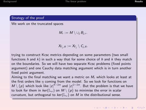
Strategy of the proof
We work on the truncated spaces
Mr := M \ ∪j Bj,r .
XΓj ,R := XΓj \ Cj,R .
trying to construct Kcsc metrics depending on some parameters (two smallfunctions h and k) in such a way that for some choice of h and k they matchon the boundaries. So we will have two separate Kcsc problems (fixed pointsargument) and one Cauchy data matching argument which is in turn anotherfixed point argument.Aiming to the final matching we want a metric on Mr which looks at least atthe first orders like η coming from the model. So we look for functions onM \ {p} which look like |z |4−2m and |z |2−2m. But the problem is that we haveto look for them in ker(Lω) on M \ {p} to minimise the error in scalarcurvature, but orthogonal to ker(Lω) on M in the distributional sense.
Background The linear problem Results
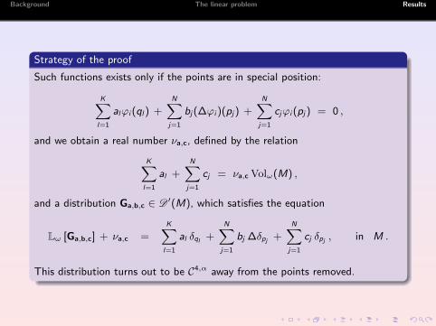
Strategy of the proof
Such functions exists only if the points are in special position:
K∑l=1
alϕi (ql) +N∑j=1
bj(∆ϕi )(pj) +N∑j=1
cjϕi (pj) = 0 ,
and we obtain a real number νa,c, defined by the relation
K∑l=1
al +N∑j=1
cj = νa,c Volω(M) ,
and a distribution Ga,b,c ∈ D ′(M), which satisfies the equation
Lω [Ga,b,c] + νa,c =K∑l=1
al δql +N∑j=1
bj ∆δpj +N∑j=1
cj δpj , in M .
This distribution turns out to be C4,α away from the points removed.
Background The linear problem Results
Strategy of the proof
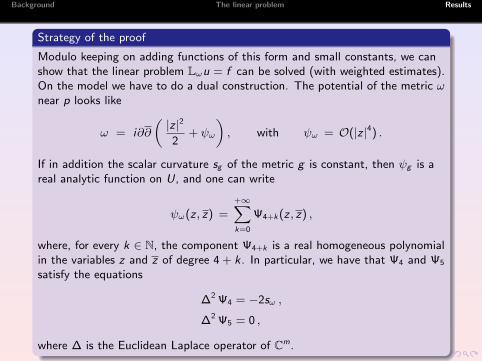
Modulo keeping on adding functions of this form and small constants, we canshow that the linear problem Lωu = f can be solved (with weighted estimates).On the model we have to do a dual construction. The potential of the metric ωnear p looks like
ω = i∂∂
(|z |2
2+ ψω
), with ψω = O(|z |4) .
If in addition the scalar curvature sg of the metric g is constant, then ψg is areal analytic function on U, and one can write
ψω(z , z) =+∞∑k=0
Ψ4+k(z , z) ,
where, for every k ∈ N, the component Ψ4+k is a real homogeneous polynomialin the variables z and z of degree 4 + k. In particular, we have that Ψ4 and Ψ5
satisfy the equations
∆2 Ψ4 = −2sω ,
∆2 Ψ5 = 0 ,
where ∆ is the Euclidean Laplace operator of Cm.

Background The linear problem Results
Strategy of the proof
We have to transplant Ψ4 and Ψ5 (with a cutoff) on XΓ and at the same timeψη on M.There are many new (solvable!) technical difficulties, but all this works andgive Kcsc metrics on the truncated spaces very close to each other.Yet the final fixed point argument (the matching on the two sides) work only ifcj = sωbj !.So we understand where each condition enters in the construction....
Background The linear problem Results
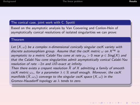
The conical case, joint work with C. Spotti
Based on the asymptotic analysis by Van Coevering and Conlon-Hein ofasymptotically conical resolutions of isolated singularities we can prove:
Theorem
Let (X , ω) be a complex n-dimensional conically singular cscK variety withdiscrete automorphism group. Assume that the cscK metric ω on X reg isasymptotic to a metric Calabi-Yau cone at rate µp > 0 near p ∈ Sing(X ) andthat the Calabi-Yau cone singularities admit asymptotically conical Calabi-Yauresolution of rate −2n and i∂∂-exact at infinity.Then there exists a crepant resolution X of X admitting a family of smoothcscK metric ωλ, for a parameter λ ∈ R small enough. Moreover, the cscKmanifolds (X , ωλ) converge to the singular cscK space (X , ω) in theGromov-Hausdorff topology as λ tends to zero.