Lecture 16 - mycourses.aalto.fi

ELEC-E4130Lecture 16: Rectangular Waveguides

Ch. 10

ELEC-E4130 / Taylor

Nov. 9, 2020

ELEC-E4130 / TaylorLecture 16

TE modes


Recall from last time

Hj

kωε

𝜕E𝜕y β

𝜕H𝜕x

Hj

kωε

𝜕E𝜕x β

𝜕H𝜕y

Ej

kωμ

𝜕H𝜕y β

𝜕E𝜕x

Ej

kωμ

𝜕H𝜕x β

𝜕E𝜕y

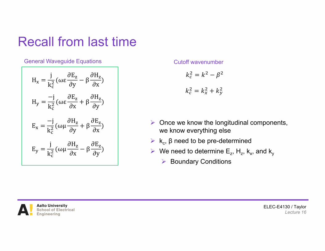
General Waveguide Equations

Once we know the longitudinal components, we know everything else

kc, β need to be pre-determined We need to determine Ez, Hz, kx, and ky

Boundary Conditions

𝑘 𝑘 𝛽

𝑘 𝑘 𝑘

Cutoff wavenumber


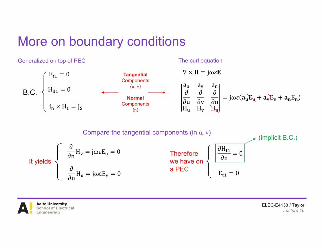
More on boundary conditionsGeneralized on top of PEC

E 0

i H J

H 0B.C.

∇ 𝐇 jωε𝐄

a a a∂∂u

∂∂v

∂∂n

H H Hjωε 𝐚𝐮E 𝐚𝐯E 𝐚𝐧E

The curl equation

TangentialComponents

(u, v)

NormalComponents

(n)

∂H∂n 0

∂∂n H jωεE 0

It yields∂∂n H jωεE 0

Thereforewe have ona PEC E 0

Compare the tangential components (in u, v)(implicit B.C.)


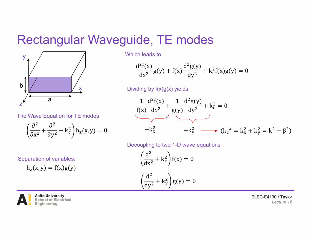
Rectangular Waveguide, TE modesy

x

z

b

a

𝜕𝜕x

𝜕𝜕y k h x, y 0

h x, y f x g yd

dy k g y 0

ddx k f x 0

k k k k β

Separation of variables:

The Wave Equation for TE modes

d f xdx g y f x

d g ydy k f x g y 0

Which leads to,

Dividing by f(x)g(x) yields,

1f x

d f xdx

1g y

d g ydy k 0

k k

Decoupling to two 1-D wave equations



x

z

b

a

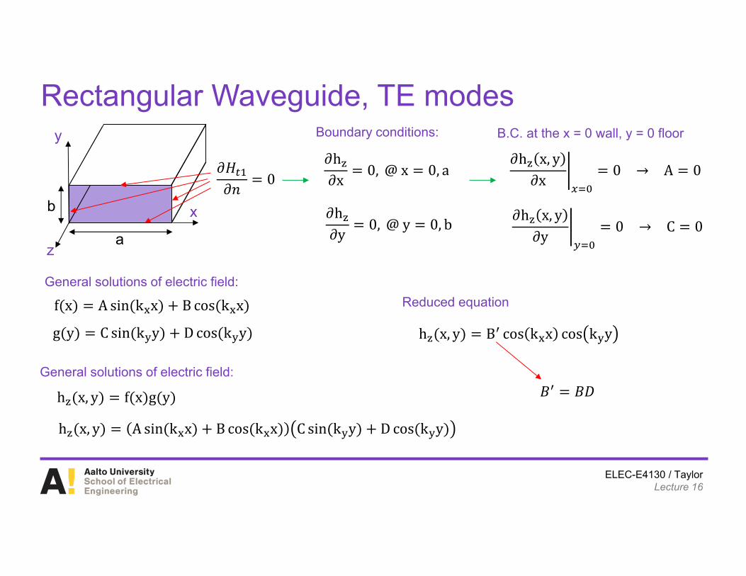
General solutions of electric field:

f x A sin k x B cos k x

g y C sin k y D cos k y

h x, y f x g y

General solutions of electric field:

h x, y A sin k x B cos k x C sin k y D cos k y

𝜕h𝜕x 0, @ x 0, a

Boundary conditions:

𝜕h𝜕y 0, @ y 0, b

𝜕𝐻𝜕𝑛 0

𝜕h x, y𝜕x 0 → A 0

B.C. at the x = 0 wall, y = 0 floor

𝜕h x, y𝜕y 0 → C 0

𝐵 𝐵𝐷

Reduced equation

h x, y B cos k x cos k y



x

z

b

a

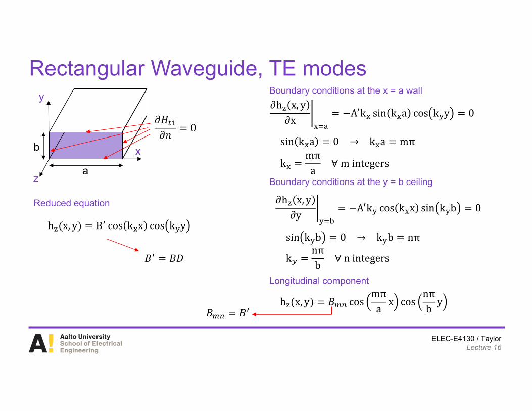
Boundary conditions at the x = a wall

Reduced equation

sin k a 0 → k a mπ

kmπ

a ∀ m integers

Boundary conditions at the y = b ceiling

Longitudinal component

h x, y 𝐵 cosmπ

a x cosnπb y

𝐵 𝐵

𝜕𝐻𝜕𝑛 0

𝐵 𝐵𝐷

h x, y B cos k x cos k y

𝜕h x, y𝜕x A k sin k a cos k y 0

sin k b 0 → k b nπ

knπb ∀ n integers

𝜕h x, y𝜕y A k cos k x sin k b 0



x

z

b

a

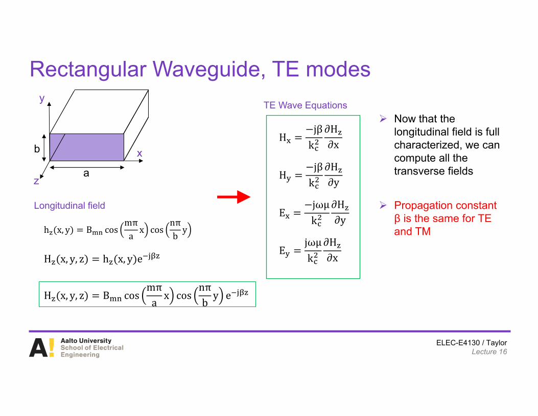
Longitudinal field

h x, y B cosmπ

a x cosnπb y

H x, y, z h x, y e

H x, y, z B cosmπ

a x cosnπb y e

Now that the longitudinal field is full characterized, we can compute all the transverse fields

Propagation constant β is the same for TE and TM

TE Wave Equations

Hjβ

k∂H∂x

Hjβ

k∂H∂y

Ejωμk

∂H∂y

Ejωμk

∂H∂x


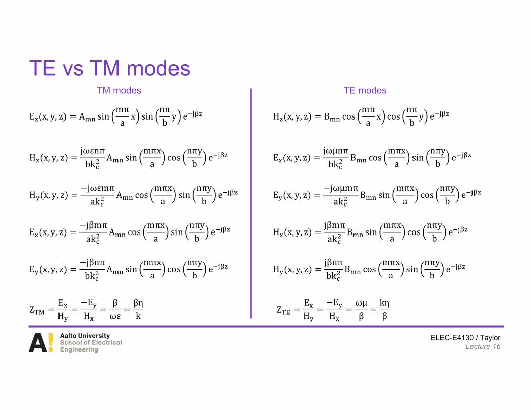
TE vs TM modes

E x, y, z A sinmπ

a x sinnπb y e

H x, y, zjωεnπ

bkA sin

mπxa cos

nπyb e

H x, y, zjωεmπak

A cosmπx

a sinnπy

b e

E x, y, zjβnπbk

A sinmπx

a cosnπy

b e

E x, y, zjβmπak

A cosmπx

a sinnπy

b e H x, y, zjβmπak

B sinmπx

a cosnπy

b e

H x, y, zjβnπbk

B cosmπx

a sinnπy

b e

E x, y, zjωμmπak

B sinmπx

a cosnπy

b e

E x, y, zjωμnπ

bkB cos

mπxa sin

nπyb e

H x, y, z B cosmπ

a x cosnπb y e

ZEH

EH

βωε

βηk Z

EH

EH

ωμβ

kηβ

TM modes TE modes


Cutoff Frequencies


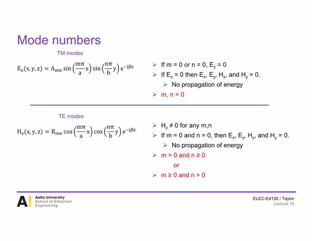
Mode numbers

E x, y, z A sinmπ

a x sinnπb y e

H x, y, z B cosmπ

a x cosnπb y e

TM modes

TE modes

If m = 0 or n = 0, Ez = 0 If Ez = 0 then Ex, Ey, Hx, and Hy = 0. No propagation of energy

m, n > 0

Hz ≠ 0 for any m,n If m = 0 and n = 0, then Ex, Ey, Hx, and Hy = 0. No propagation of energy

m > 0 and n ≥ 0or

m ≥ 0 and n > 0


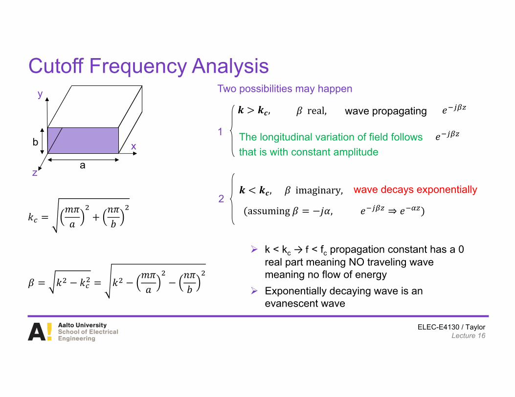
Cutoff Frequency Analysis

𝛽 𝑘 𝑘 𝑘𝑚𝜋𝑎

𝑛𝜋𝑏

𝑘𝑚𝜋𝑎

𝑛𝜋𝑏

Two possibilities may happeny

x

z

b

a

𝒌 𝒌𝒄, 𝛽 real, wave propagating 𝑒

The longitudinal variation of field followsthat is with constant amplitude

𝑒1

𝒌 𝒌𝒄, 𝛽 imaginary, wave decays exponentially

assuming 𝛽 𝑗𝛼, 𝑒 ⇒ 𝑒2

k < kc → f < fc propagation constant has a 0 real part meaning NO traveling wave meaning no flow of energy

Exponentially decaying wave is an evanescent wave


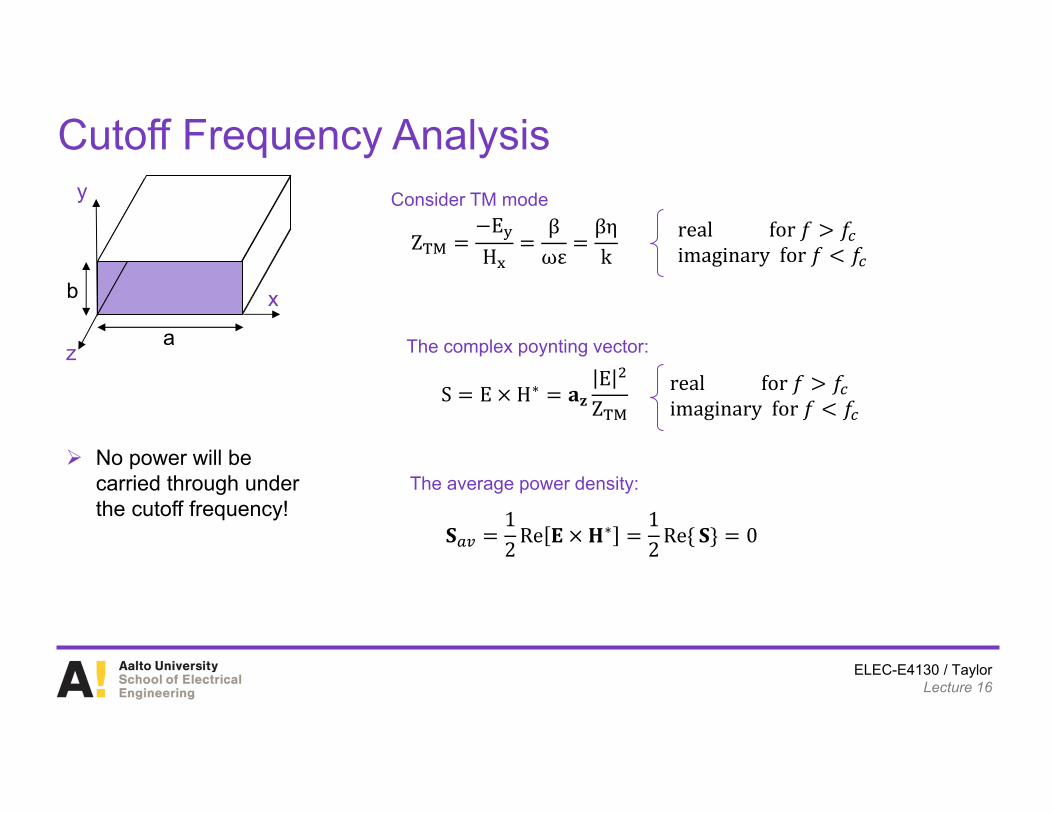
Cutoff Frequency Analysisy

x

z

b

a

Consider TM mode

ZE

Hβωε

βηk

real for 𝑓 𝑓imaginary for 𝑓 𝑓

The complex poynting vector:

𝐒12 Re 𝐄 𝐇∗ 1

2 Re 𝐒 0

The average power density:

S E H∗ 𝐚𝐳E

Zreal for 𝑓 𝑓imaginary for 𝑓 𝑓

No power will be carried through under the cutoff frequency!


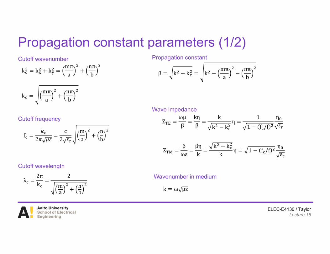
Propagation constant parameters (1/2)

kmπ

anπb

k ω με

f𝑘

2𝜋 𝜇𝜀c

2 εma

nb

β k k kmπ

anπb

k k kmπ

anπb

λ2πk

2

ma

nb

Cutoff wavenumber

Cutoff frequency

Cutoff wavelength

Propagation constant

Zωμβ

kηβ

k

k kη

11 f /f

ηε

Zβωε

βηk

k kk η 1 f /f

ηε

Wave impedance

Wavenumber in medium


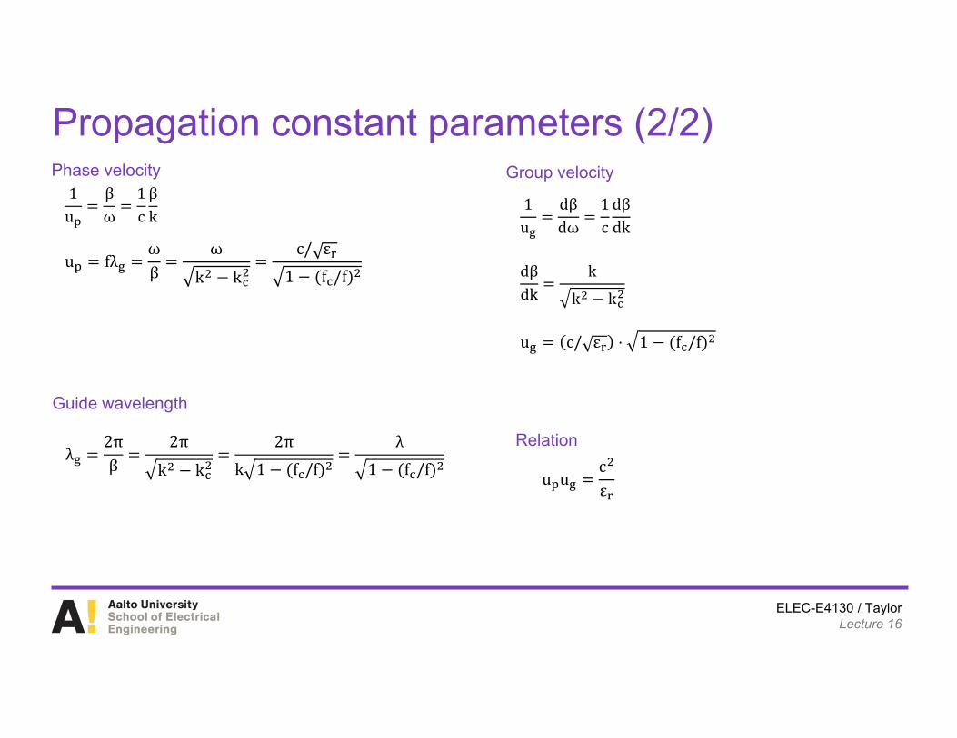
Propagation constant parameters (2/2)

Guide wavelength

λ2πβ

2π

k k

2πk 1 f /f

λ1 f /f

u fλωβ

ω

k k

c/ ε1 f /f

u c/ ε ⋅ 1 f /f

1u

dβdω

1c

dβdk

1u

βω

1cβk

dβdk

k

k k

Phase velocity Group velocity

u ucε

Relation


In class exercise: Cutoff Frequenciesy

x

z

b

a

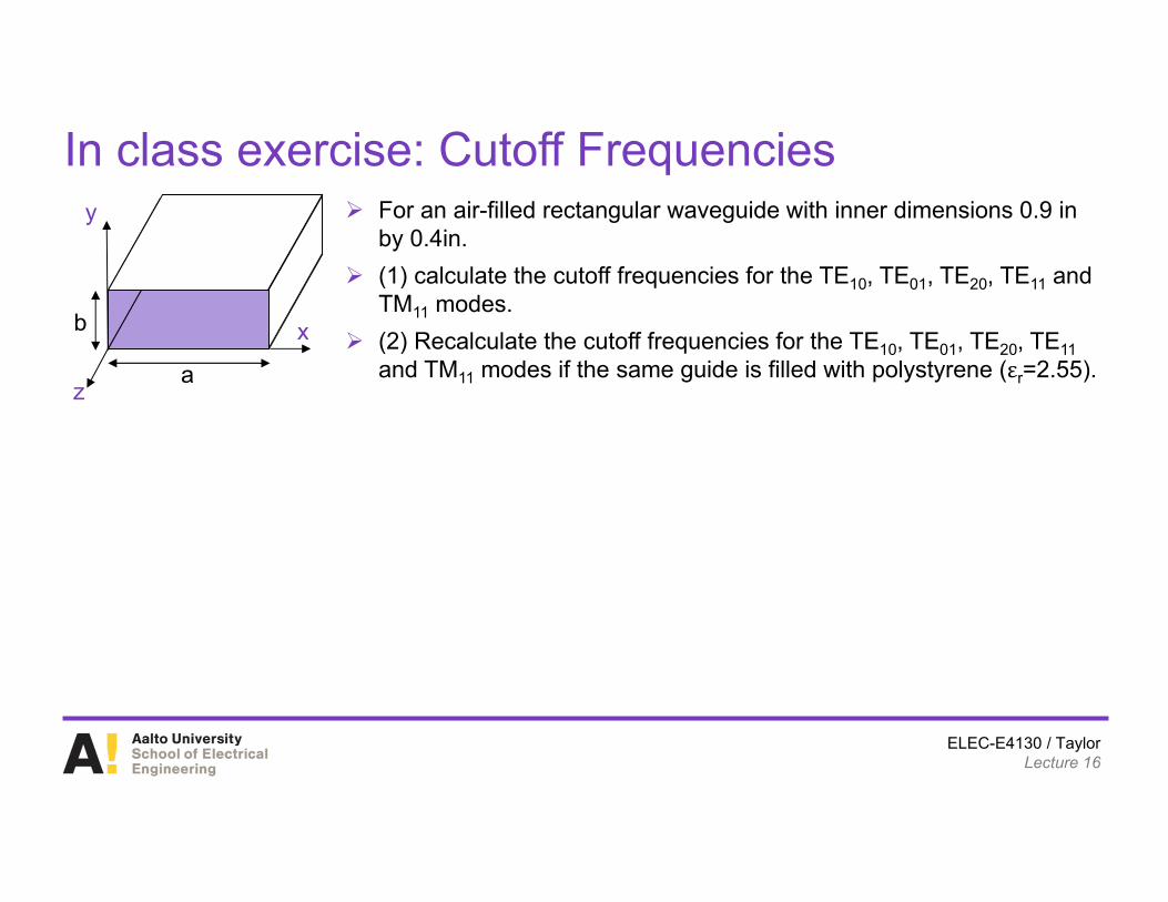
For an air-filled rectangular waveguide with inner dimensions 0.9 in by 0.4in.

(1) calculate the cutoff frequencies for the TE10, TE01, TE20, TE11 and TM11 modes.

(2) Recalculate the cutoff frequencies for the TE10, TE01, TE20, TE11and TM11 modes if the same guide is filled with polystyrene (εr=2.55).



x

z

b

a

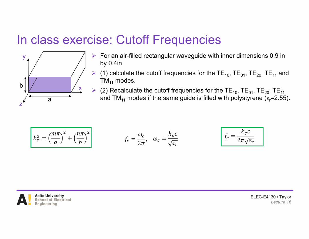
For an air-filled rectangular waveguide with inner dimensions 0.9 in by 0.4in.

(1) calculate the cutoff frequencies for the TE10, TE01, TE20, TE11 and TM11 modes.

(2) Recalculate the cutoff frequencies for the TE10, TE01, TE20, TE11and TM11 modes if the same guide is filled with polystyrene (εr=2.55).

𝜔𝑘 𝑐𝜀𝑓

𝜔2𝜋 , 𝑓

𝑘 𝑐2𝜋 𝜀𝑘

𝑚𝜋𝑎

𝑛𝜋𝑏


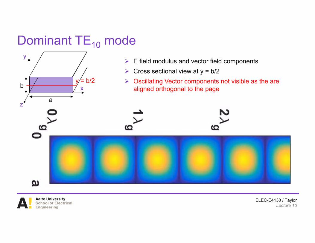
Dominant TE10 mode


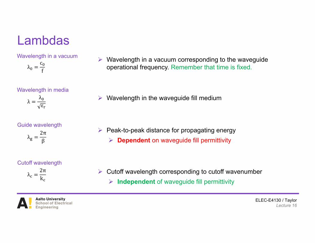
Lambdas

Guide wavelength

λ2πβ

Wavelength in a vacuum

λcf

Wavelength in media

λλε

λ2πk

Cutoff wavelength

Wavelength in a vacuum corresponding to the waveguide operational frequency. Remember that time is fixed.

Wavelength in the waveguide fill medium

Peak-to-peak distance for propagating energy Dependent on waveguide fill permittivity

Cutoff wavelength corresponding to cutoff wavenumber Independent of waveguide fill permittivity


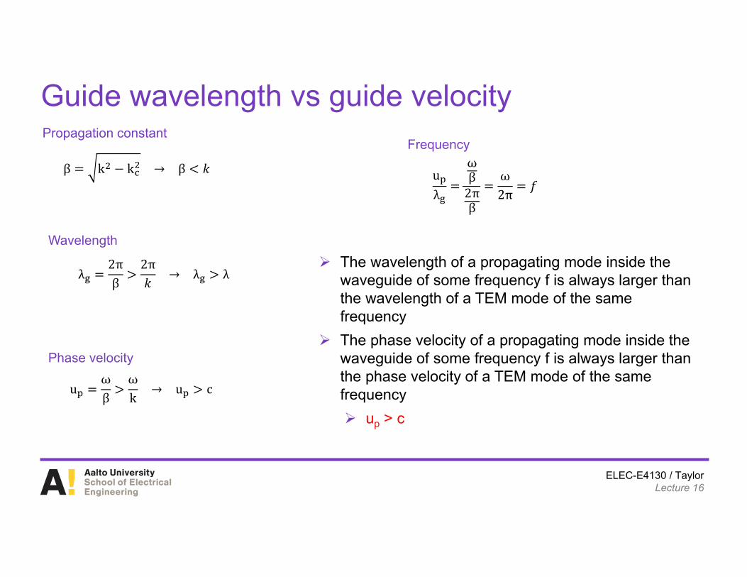
Guide wavelength vs guide velocityPropagation constant

The wavelength of a propagating mode inside the waveguide of some frequency f is always larger than the wavelength of a TEM mode of the same frequency

The phase velocity of a propagating mode inside the waveguide of some frequency f is always larger than the phase velocity of a TEM mode of the same frequency up > c

β k k → β 𝑘

λ2πβ

2π𝑘 → λ λ

Wavelength

uωβ

ωk → u c

Phase velocity

uλ

ωβ

2πβ

ω2π 𝑓

Frequency


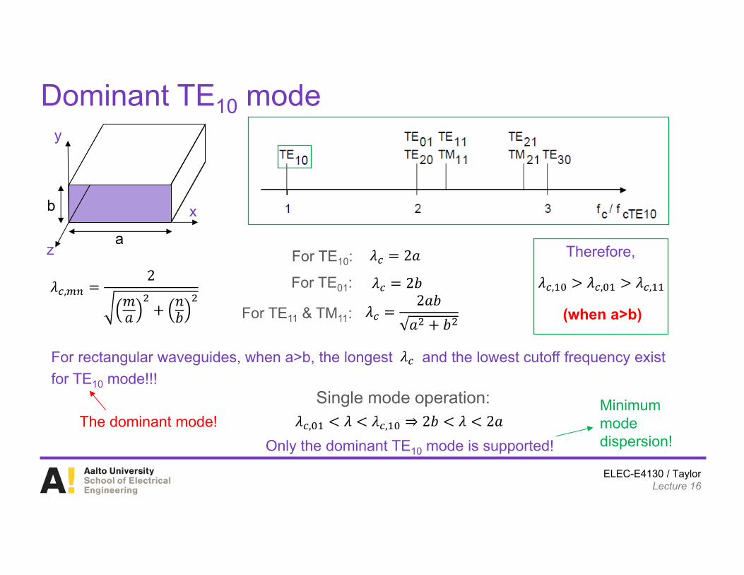
Dominant TE10 mode

𝜆 ,2

𝑚𝑎

𝑛𝑏

𝜆 2𝑏

𝜆 2𝑎For TE10:

For TE01:

For TE11 & TM11: 𝜆2𝑎𝑏𝑎 𝑏

For rectangular waveguides, when a>b, the longest and the lowest cutoff frequency exist for TE10 mode!!!

𝜆

The dominant mode!Single mode operation:

𝜆 , 𝜆 𝜆 , ⇒ 2𝑏 𝜆 2𝑎Only the dominant TE10 mode is supported!

Minimum mode dispersion!

Therefore,

𝜆 , 𝜆 , 𝜆 ,

(when a>b)

y

x

z

b

a


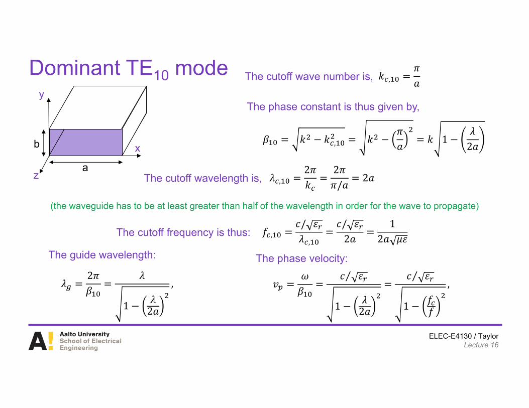
Dominant TE10 mode

𝛽 𝑘 𝑘 , 𝑘𝜋𝑎 𝑘 1

𝜆2𝑎

𝜆 ,2𝜋𝑘

2𝜋𝜋/𝑎 2𝑎

𝜆2𝜋𝛽

𝜆

1 𝜆2𝑎

, 𝑣𝜔𝛽

𝑐 𝜀⁄

1 𝜆2𝑎

𝑐 𝜀⁄

1 𝑓𝑓

,

The phase constant is thus given by,

The cutoff wavelength is,

𝑓 ,𝑐/ 𝜀𝜆 ,

𝑐/ 𝜀2𝑎

12𝑎 𝜇𝜀

The cutoff wave number is, 𝑘 ,𝜋𝑎

(the waveguide has to be at least greater than half of the wavelength in order for the wave to propagate)

The cutoff frequency is thus:

The guide wavelength: The phase velocity:

y

x

z

b

a


Dominant TE10 modey

x

z

b

a

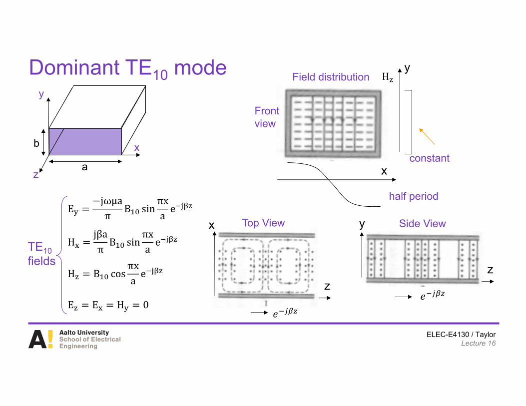
Field distribution Hy

x

half period

constant

Frontview

H B cosπxa e

E E H 0

Hjβaπ B sin

πxa e

Ejωμaπ B sin

πxa e

TE10fields

Top View

𝑒

z

x

𝑒

y

z

Side View


Dominant TE10 modey

x

z

b

a

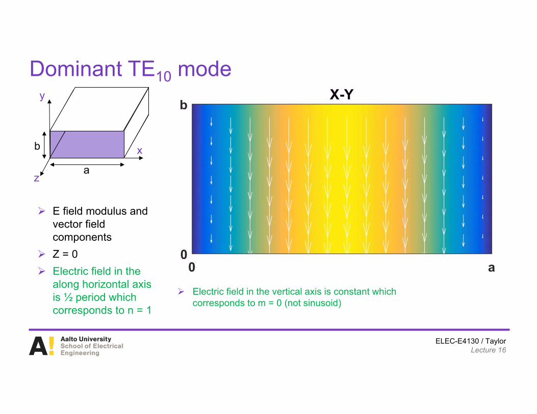
E field modulus and vector field components

Z = 0 Electric field in the

along horizontal axis is ½ period which corresponds to n = 1

Electric field in the vertical axis is constant which corresponds to m = 0 (not sinusoid)


Dominant TE10 modey

x

z

b

a

E field modulus and vector field components Cross sectional view at y = b/2 Oscillating Vector components not visible as the are

aligned orthogonal to the pagey = b/2


Dominant TE10 modey

x

z

b

a

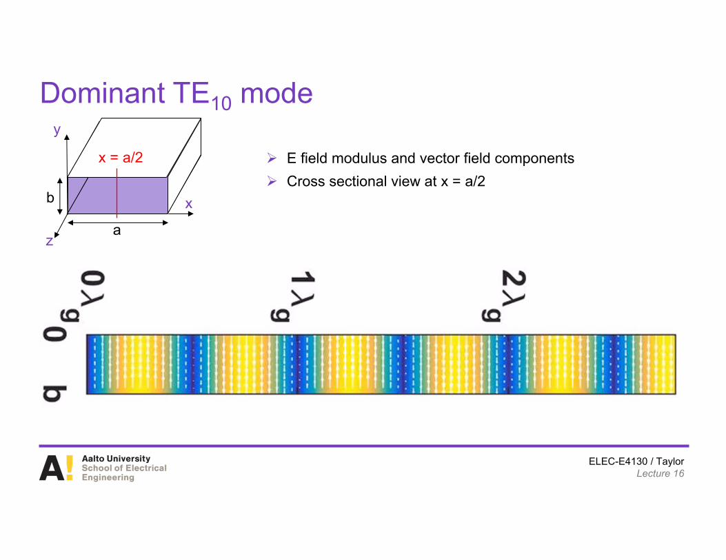
E field modulus and vector field components Cross sectional view at x = a/2

x = a/2



x

z

b

a

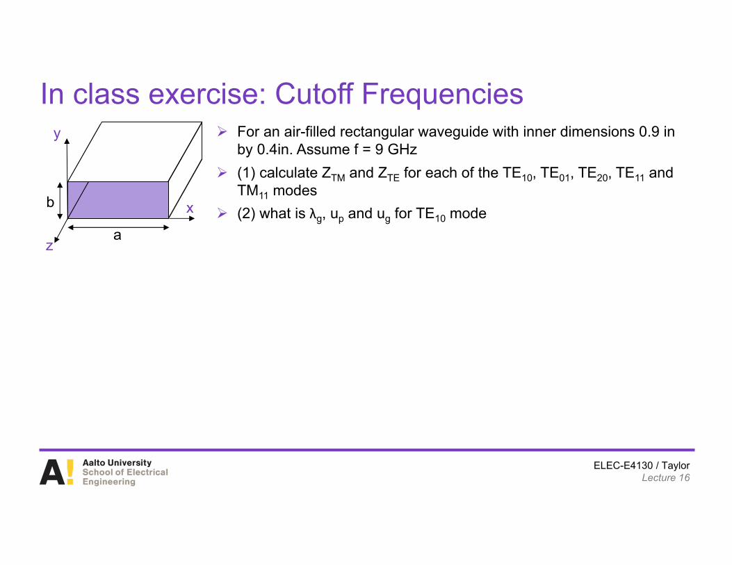
For an air-filled rectangular waveguide with inner dimensions 0.9 in by 0.4in. Assume f = 9 GHz

(1) calculate ZTM and ZTE for each of the TE10, TE01, TE20, TE11 and TM11 modes

(2) what is λg, up and ug for TE10 mode



x

z

b

a

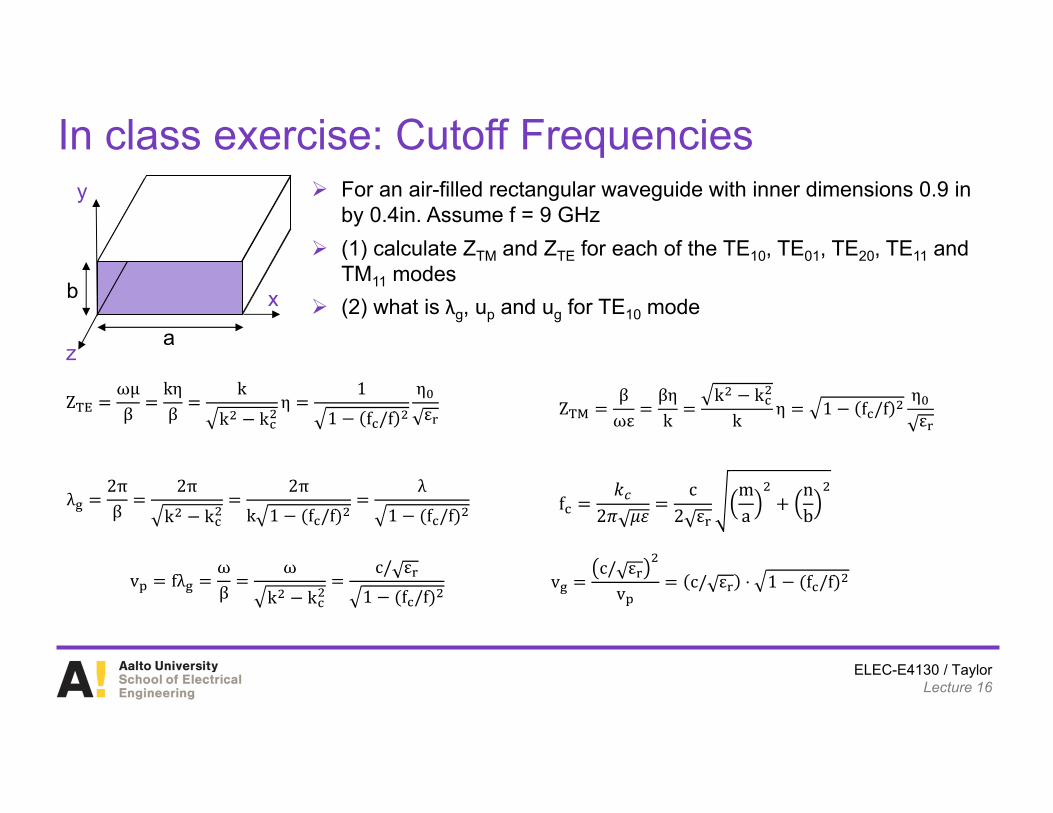
For an air-filled rectangular waveguide with inner dimensions 0.9 in by 0.4in. Assume f = 9 GHz

(1) calculate ZTM and ZTE for each of the TE10, TE01, TE20, TE11 and TM11 modes

(2) what is λg, up and ug for TE10 mode

Zωμβ

kηβ

k

k kη

11 f /f

ηε Z

βωε

βηk

k kk

η 1 f /fηε

λ2πβ

2π

k k

2πk 1 f /f

λ1 f /f

v fλωβ

ω

k k

c/ ε1 f /f

vc/ ε

vc/ ε ⋅ 1 f /f

f𝑘

2𝜋 𝜇𝜀c

2 εma

nb


Conclusions


Real WGy

x

z

b

a

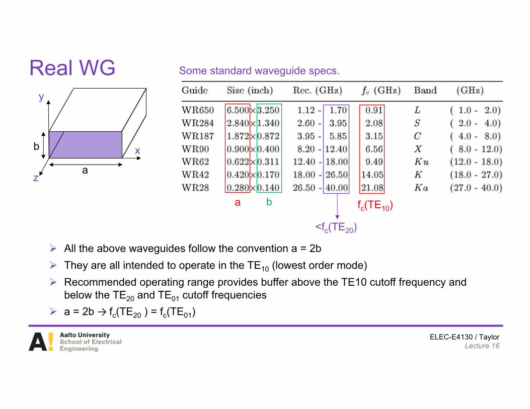
All the above waveguides follow the convention a = 2b They are all intended to operate in the TE10 (lowest order mode) Recommended operating range provides buffer above the TE10 cutoff frequency and

below the TE20 and TE01 cutoff frequencies a = 2b → fc(TE20 ) = fc(TE01)

Some standard waveguide specs.

a b fc(TE10)

<fc(TE20)


Propagationy

x

z

b

a

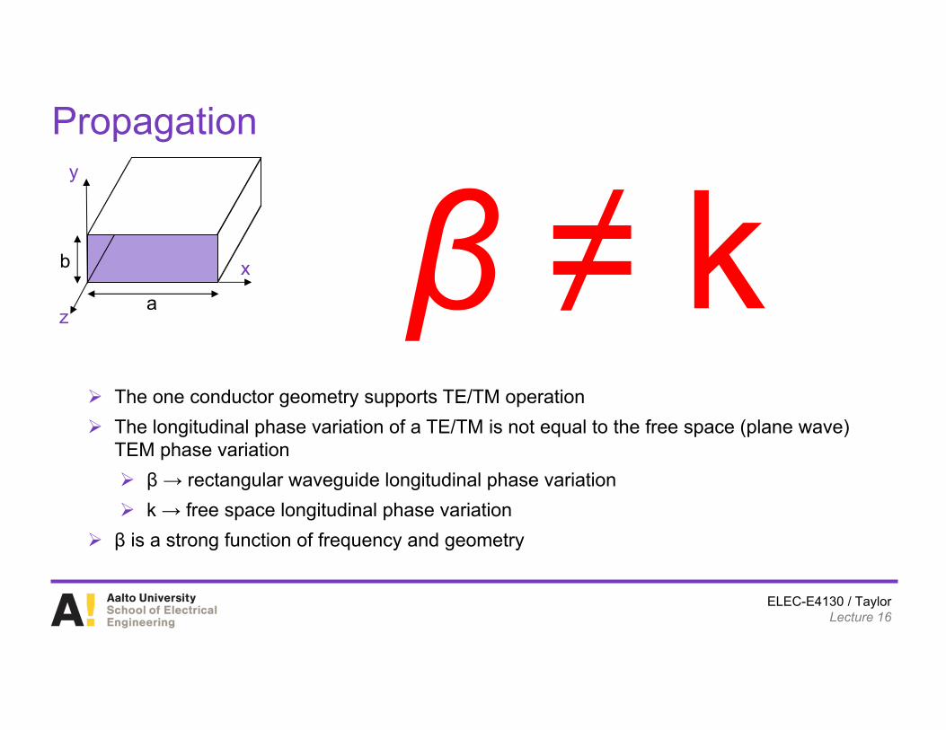
The one conductor geometry supports TE/TM operation The longitudinal phase variation of a TE/TM is not equal to the free space (plane wave)

TEM phase variation β → rectangular waveguide longitudinal phase variation k → free space longitudinal phase variation

β is a strong function of frequency and geometry


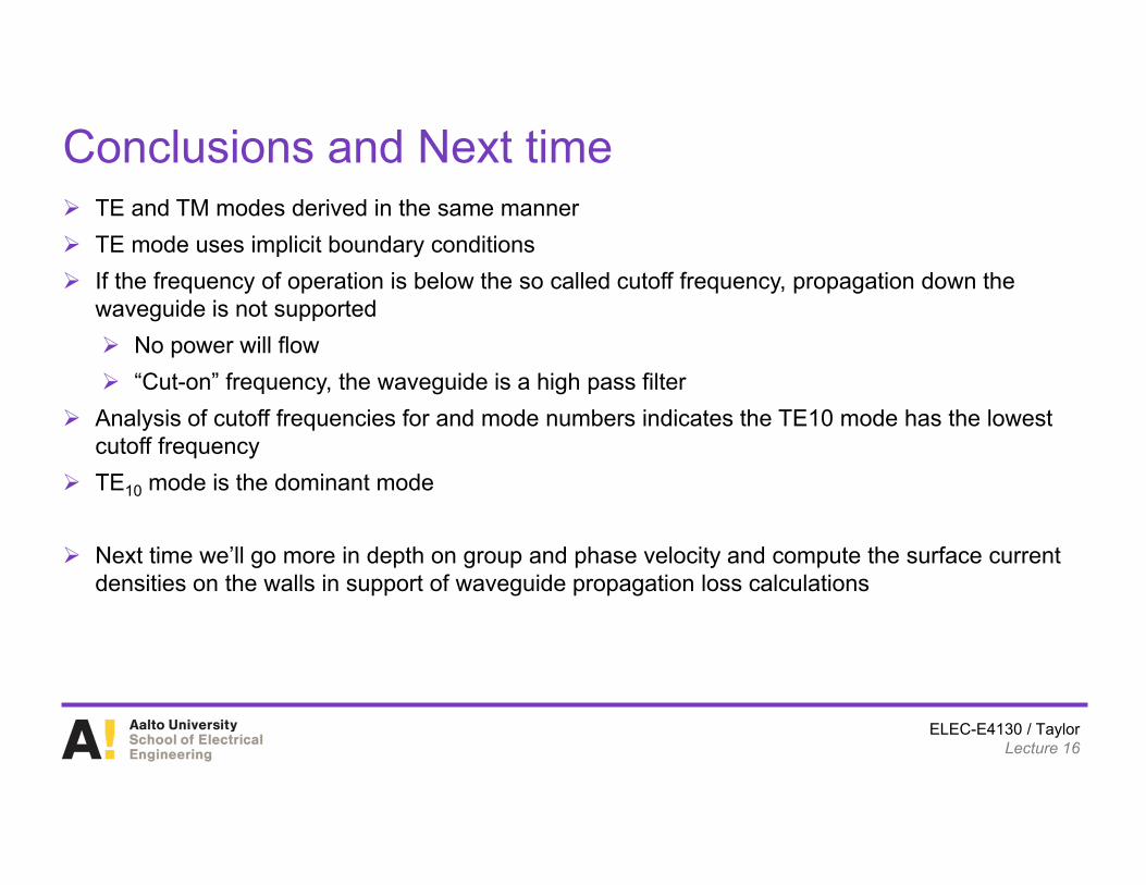
Conclusions and Next time TE and TM modes derived in the same manner TE mode uses implicit boundary conditions If the frequency of operation is below the so called cutoff frequency, propagation down the

waveguide is not supported No power will flow “Cut-on” frequency, the waveguide is a high pass filter

Analysis of cutoff frequencies for and mode numbers indicates the TE10 mode has the lowest cutoff frequency

TE10 mode is the dominant mode

Next time we’ll go more in depth on group and phase velocity and compute the surface current densities on the walls in support of waveguide propagation loss calculations

Lecture 16 - mycourses.aalto.fi

Documents

Transcript of Lecture 16 - mycourses.aalto.fi