EE16B - Fall’16 - Lecture 11A Notes11 Licensed under a Creative CommonsAttribution-NonCommercial-ShareAlike4.0 International License.Murat Arcak

8 November 2016

Interpolation with Basis Functions

Recall that in this method we assign to each xi a function φi(x) thatsatisfies:

φi(xi) = 1 and φi(xj) = 0 when j 6= i (1)

and interpolate between the data points (xi, yi) with the function:

y = ∑k

ykφk(x). (2)

When x = xi this expression yields y = yi as desired, becauseφk(xi) = 0 except when k = i.

We refer to φi(x) as “basis functions" since our interpolation is ob-tained from a linear combination of these functions. Basis functionsrestrict the behavior of the interpolation between the data points,thus avoiding the erratic results of polynomial interpolation.

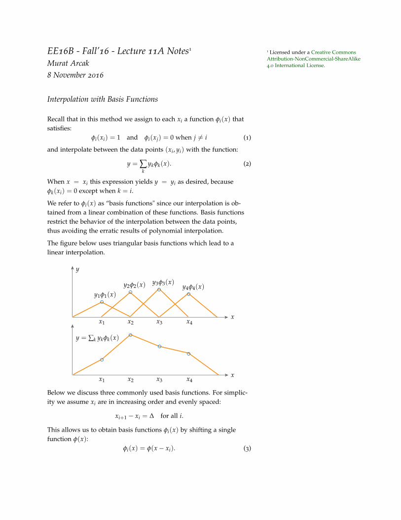
The figure below uses triangular basis functions which lead to alinear interpolation.

x

x

y

x1 x2 x3 x4

x1 x2 x3 x4

y1φ1(x)y2φ2(x) y3φ3(x)

y4φ4(x)

y = ∑k ykφk(x)

Below we discuss three commonly used basis functions. For simplic-ity we assume xi are in increasing order and evenly spaced:

xi+1 − xi = ∆ for all i.

This allows us to obtain basis functions φi(x) by shifting a singlefunction φ(x):

φi(x) = φ(x− xi). (3)

ee16b - fall’16 - lecture 11a notes 2

Note that (1) holds if we define φ(x) such that

φ(0) = 1 and φ(k∆) = 0 when k 6= 0. (4)

Linear Interpolation

x

∆−∆

1

When φ(x) is as depicted on the right, that is

φ(x) =

{1− |x|∆ |x| ≤ ∆0 otherwise,

and the basis functions are obtained from (3), then the interpolation(2) connects the data points with straight lines. (See figure above.)

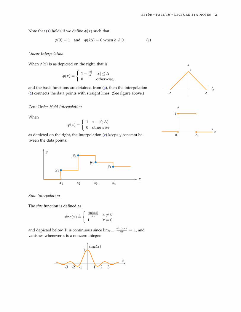
Zero Order Hold Interpolation

x

∆0

1When

φ(x) =

{1 x ∈ [0, ∆)0 otherwise

as depicted on the right, the interpolation (2) keeps y constant be-tween the data points:

x

y

x1 x2 x3 x4

y1

y2

y3y4

Sinc Interpolation

The sinc function is defined as

sinc(x) ,

{sin(πx)

πx x 6= 01 x = 0

and depicted below. It is continuous since limx→0sin(πx)

πx = 1, andvanishes whenever x is a nonzero integer.

-3 -2 -1 1 2 3

1

x

sinc(x)

ee16b - fall’16 - lecture 11a notes 3

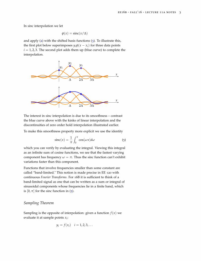
In sinc interpolation we let

φ(x) = sinc(x/∆)

and apply (2) with the shifted basis functions (3). To illustrate this,the first plot below superimposes yiφ(x − xi) for three data pointsi = 1, 2, 3. The second plot adds them up (blue curve) to complete theinterpolation.

∆ 2∆ 3∆

y1

y2 y3

x

∆ 2∆ 3∆

x

The interest in sinc interpolation is due to its smoothness – contrastthe blue curve above with the kinks of linear interpolation and thediscontinuities of zero order hold interpolation illustrated earlier.

To make this smoothness property more explicit we use the identity

sinc(x) =1π

∫ π

0cos(ωx)dω (5)

which you can verify by evaluating the integral. Viewing this integralas an infinite sum of cosine functions, we see that the fastest varyingcomponent has frequency ω = π. Thus the sinc function can’t exhibitvariations faster than this component.

Functions that involve frequencies smaller than some constant arecalled “band-limited." This notion is made precise in EE 120 withcontinuous Fourier Transforms. For 16B it is sufficient to think of aband-limited signal as one that can be written as a sum or integral ofsinusoidal components whose frequencies lie in a finite band, whichis [0, π] for the sinc function in (5).

Sampling Theorem

Sampling is the opposite of interpolation: given a function f (x) weevaluate it at sample points xi:

yi = f (xi) i = 1, 2, 3, . . .

ee16b - fall’16 - lecture 11a notes 4

Sampling is critical in digital signal processing where one uses sam-ples of an analog sound or image. For example, digital audio is oftenrecorded at 44.1 kHz which means that the analog audio is sampled44,100 times per second; these samples are then used to reconstructthe audio when playing it back. Similarly, in digital images each pixelcorresponds to a sample of an analog image.

An important problem in sampling is whether we can perfectly re-cover an analog signal from its samples. As we explain below, theanswer is yes when the analog signal is band-limited and the intervalbetween the samples is sufficiently short.

Suppose we sample the function f : R→ R at evenly spaced points

xi = ∆i, i = 1, 2, 3, . . .

and obtainyi = f (∆i) i = 1, 2, 3, . . .

Then sinc interpolation between these data points gives:

f̂ (x) = ∑i

yiφ(x− ∆i) (6)

whereφ(x) = sinc(x/∆),

which is band-limited by π/∆ from (5). This means that f̂ (x) in (6)contains frequencies ranging from 0 to π/∆.

Now if f (x) involves frequencies smaller than π/∆, then it is reason-able to expect that it can be recovered from (6) which varies as fast asf (x). In fact the shifted sinc functions φ(x − ∆i) form a basis for thespace of functions2 that are band-limited by π/∆ and the formula (6) 2 for technical reasons this space is also

restricted to square integrable functionsis simply the representation of f (x) with respect to this basis.

Claude Shannon (1916-2001)

Harry Nyquist (1889-1976)

Sampling Theorem: If f (x) is band-limited by frequency

ωmax <π

∆(7)

then the sinc interpolation (6) recovers f (x), that is f̂ (x) = f (x).

By defining the sampling frequency ωs = 2π/∆, we can restate thecondition (7) as:

ωmax <ωs

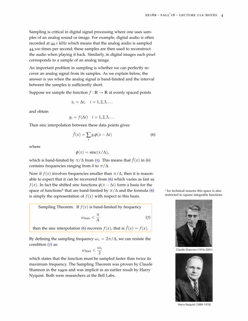
2which states that the function must be sampled faster than twice itsmaximum frequency. The Sampling Theorem was proven by ClaudeShannon in the 1940s and was implicit in an earlier result by HarryNyquist. Both were researchers at the Bell Labs.