CS774. Markov Random Field : Theory and Application

Lecture 16

Kyomin JungKAIST

Nov 03 2009

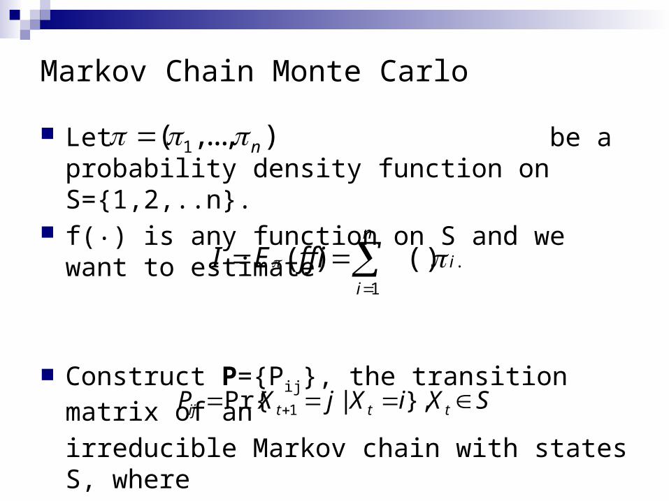
Markov Chain Monte Carlo

Let be a probability den-sity function on S={1,2,..n}.

f(‧) is any function on S and we want to es-timate

Construct P={Pij}, the transition matrix of an irreducible Markov chain with states S, where

and π is its unique stationary distribution.

1( ,..., )n

.

1

( ) ( )n

i

i

I E f f i

SXiXjXP tttij },|Pr{ 1

Markov Chain Monte Carlo

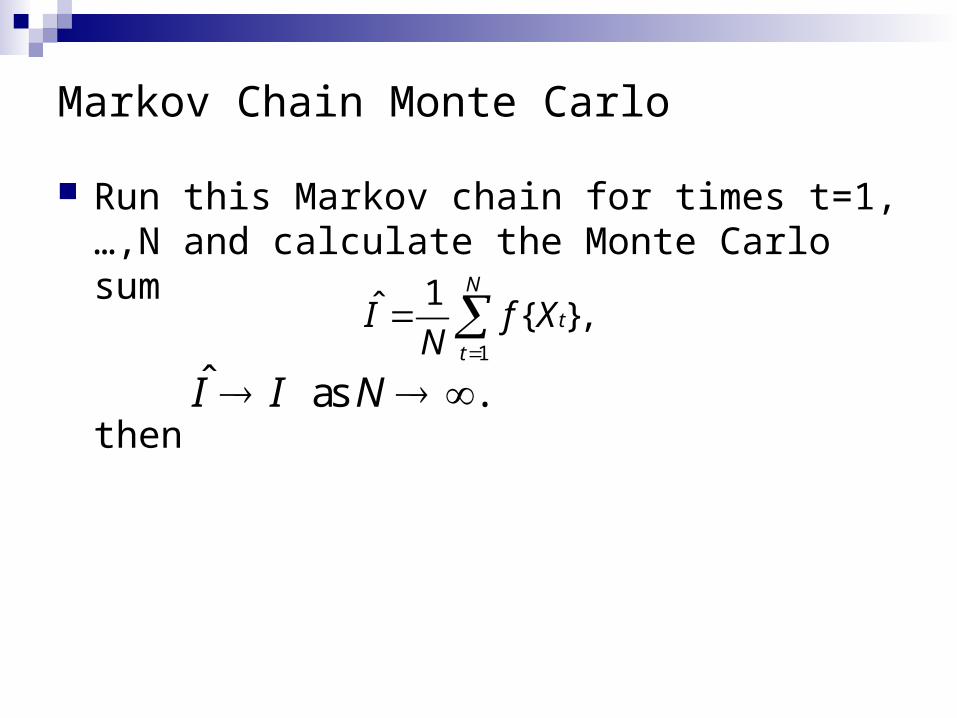
Run this Markov chain for times t=1,…,N and calculate the Monte Carlo sum

then

1

1ˆ { },N

t

t

I f XN

ˆ as .I I N

Metropolis-Hastings Algorithm

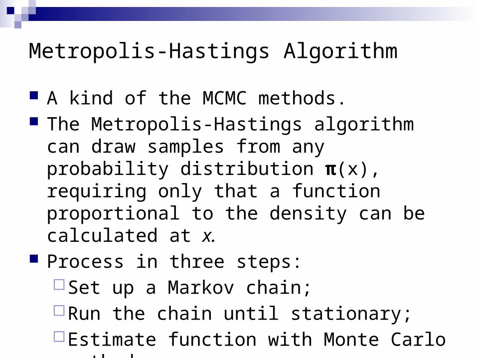
A kind of the MCMC methods. The Metropolis-Hastings algorithm can

draw samples from any probability distribu-tion π(x), requiring only that a function proportional to the density can be calcu-lated at x.

Process in three steps:Set up a Markov chain;Run the chain until stationary;Estimate function with Monte Carlo

methods.

Metropolis-Hastings Algorithm

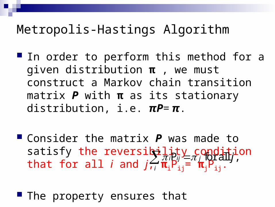
In order to perform this method for a given distribution π , we must construct a Markov chain transition matrix P with π as its sta-tionary distribution, i.e. πP= π.

Consider the matrix P was made to satisfy the reversibility condition that for all i and j, πiPij= πjPij.

The property ensures that

and hence π is the stationary distribution for P.

P for all ,i ij j

i

j

Metropolis-Hastings Algorithm

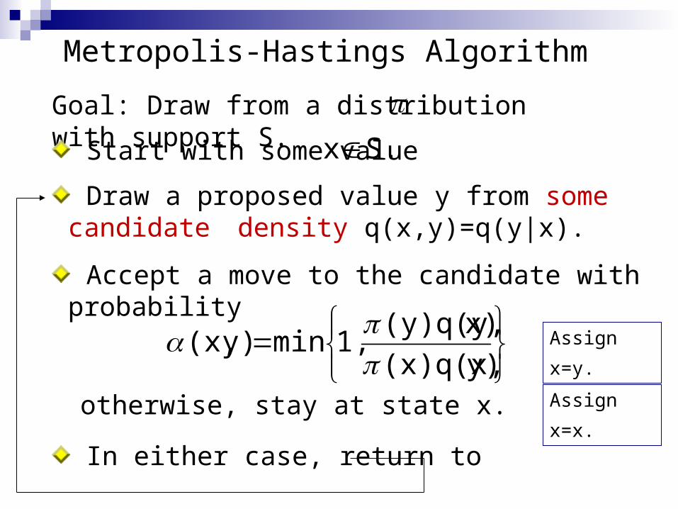
Goal: Draw from a distribution with support S. Start with some value

Draw a proposed value y from some candidate density q(x,y)=q(y|x).

Accept a move to the candidate with probability

otherwise, stay at state x.

Assign

x=y. Assign

x=x. In either case, return to

S.x

y)(x)q(x,

x)(y)q(y,1,min y)(x,

Metropolis-Hastings Algorithm

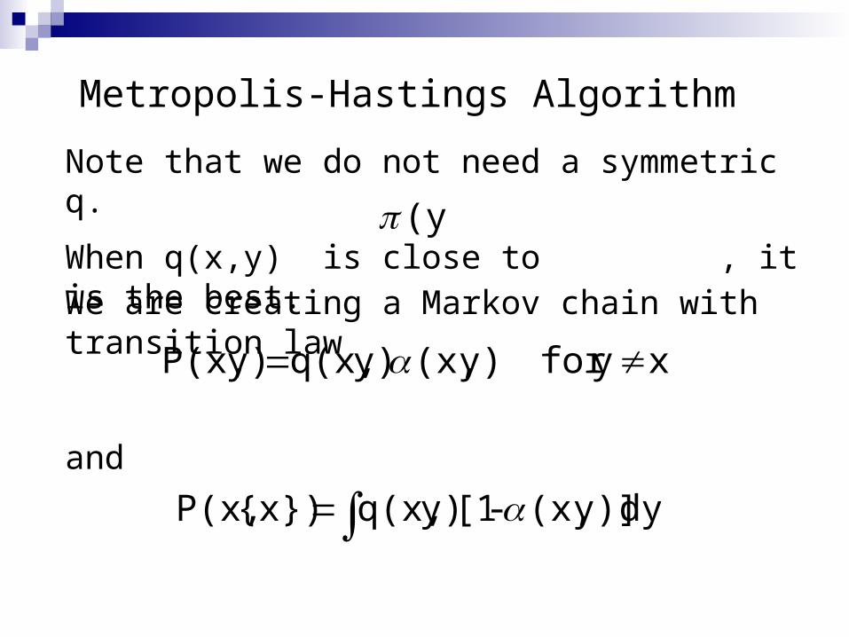
Note that we do not need a symmetric q.

When q(x,y) is close to , it is the best.

We are creating a Markov chain with transition law

and

xyfor y)(x, y)q(x, y)P(x,

dy y)](x,-[1 y)q(x, {x})P(x,

(y)

Metropolis-Hastings Algorithm

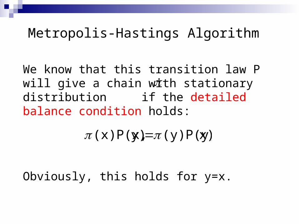
We know that this transition law P will give a chain with stationary distribution if the detailed balance condition holds:

Obviously, this holds for y=x.

x)(y)P(y,y)(x)P(x,

Metropolis-Hastings Algorithm

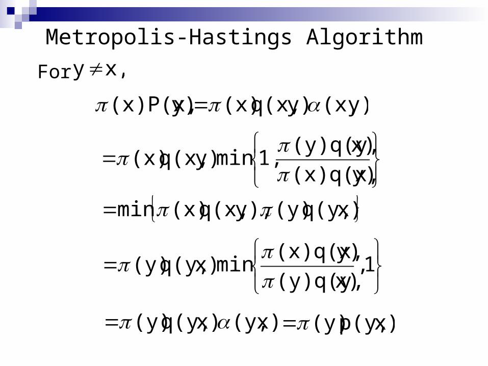
For x,y

y)(x, y)q(x, (x)y)(x)P(x,

x)q(y, (y) y),q(x, (x)min

y)(x)q(x,

x)(y)q(y,1,min y)q(x, (x)

1 ,x)(y)q(y,

y)(x)q(x,min x)q(y, (y)

x)(y, x)q(y, (y) x)p(y, (y)

Metropolis-Hastings Algorithm

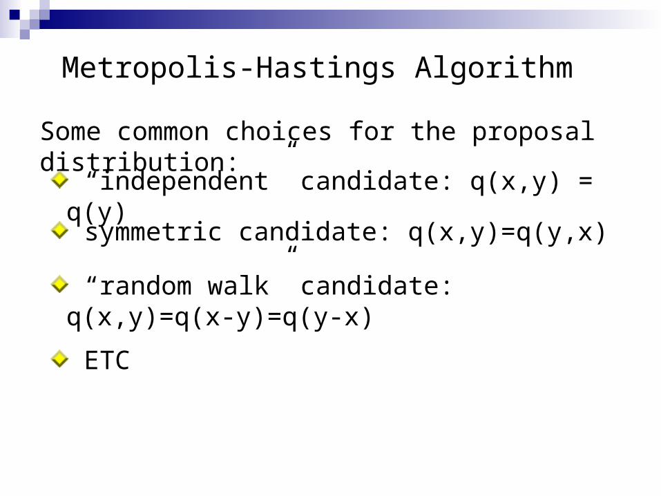
Some common choices for the proposal distribution:

“independent” candidate: q(x,y) = q(y)

symmetric candidate: q(x,y)=q(y,x)

“random walk” candidate: q(x,y)=q(x-y)=q(y-x)

ETC

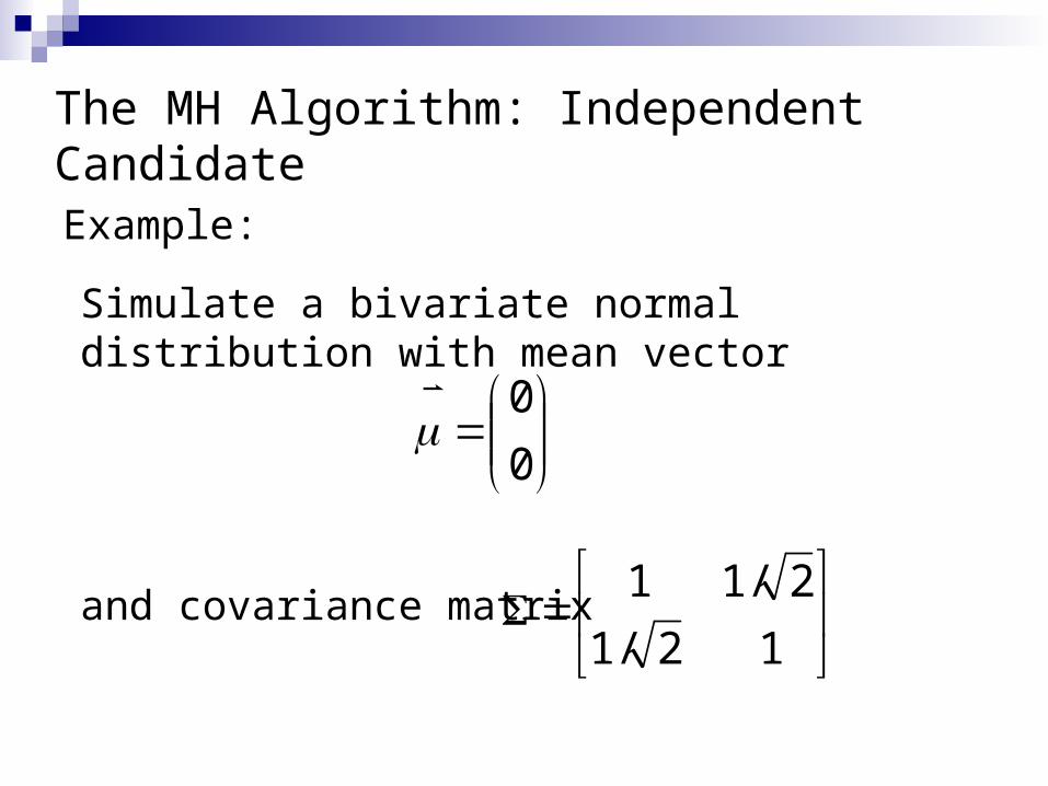
The MH Algorithm: Independent Candidate

Example:

Simulate a bivariate normal distribution with mean vector

and covariance matrix

121/

21/1

0

0

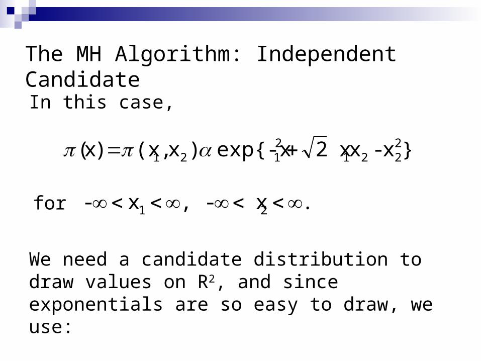
The MH Algorithm: Independent CandidateIn this case,

for

We need a candidate distribution to draw values on R2, and since exponentials are so easy to draw, we use:

}x-x x2exp{-x )x,(x)x( 2221

2121

. x - , x- 21

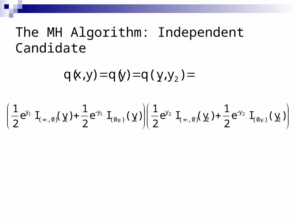
The MH Algorithm: Independent Candidate

)y,q(y )yq()y,xq( 21

)(yI e

2

1)(yI e

2

1)(yI e

2

1)(yI e

2

12)(0,

y-2,0)(-

y1)(0,

y-1,0)(-

y 2211

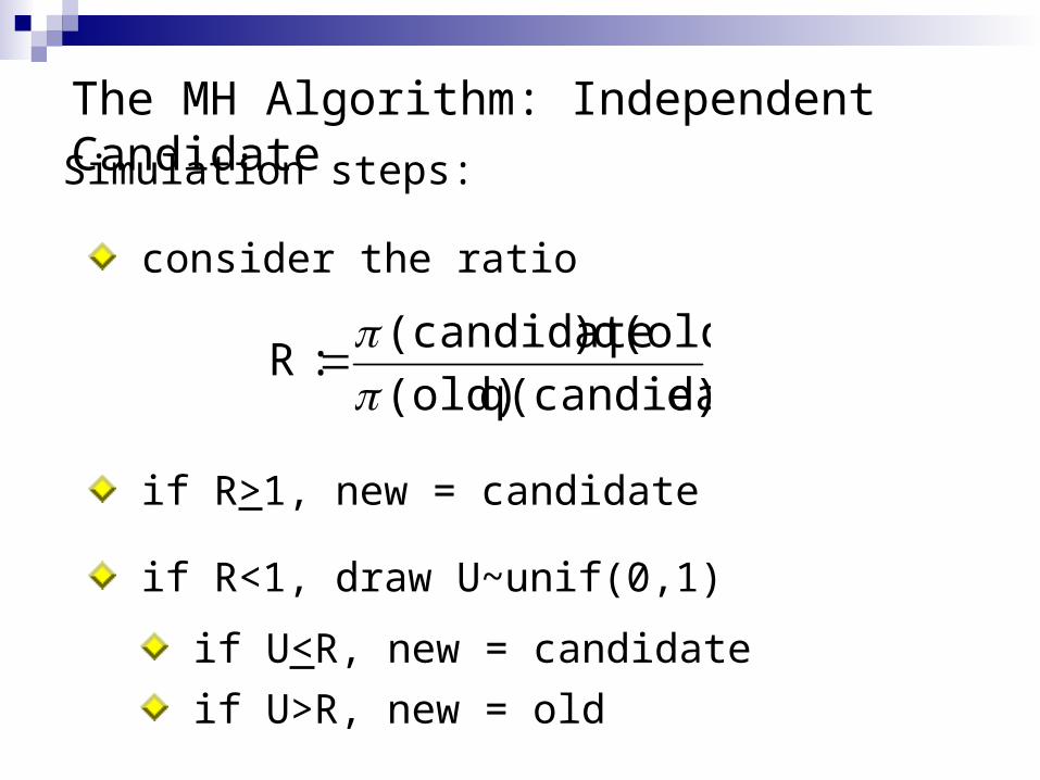
The MH Algorithm: Independent CandidateSimulation steps:

consider the ratio

if R>1, new = candidate

if R<1, draw U~unif(0,1)

if U<R, new = candidate

if U>R, new = old

e)q(candidat (old)

q(old) )(candidate:R

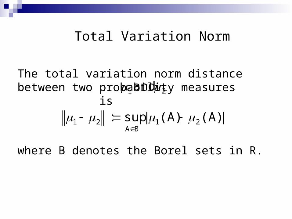
Total Variation Norm

The total variation norm distance between two probability measures is

where B denotes the Borel sets in R.

2 1 and

|(A)(A)| sup : 21A

21 B

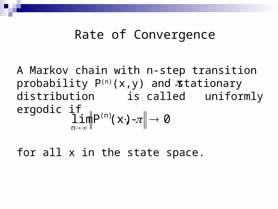
Rate of Convergence

A Markov chain with n-step transition probability P(n)(x,y) and stationary distribution is called uniformly ergodic if

for all x in the state space.

0-)(x,P lim (n)

n

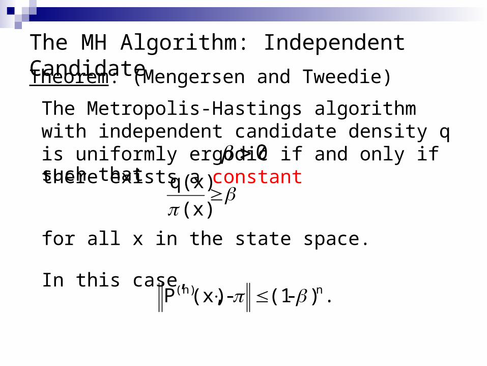
The MH Algorithm: Independent CandidateTheorem: (Mengersen and Tweedie)

The Metropolis-Hastings algorithm with independent candidate density q is uniformly ergodic if and only if there exists a constant such that

for all x in the state space.

In this case,

0

(x)

q(x)

.)-(1 -)(x,P n(n)

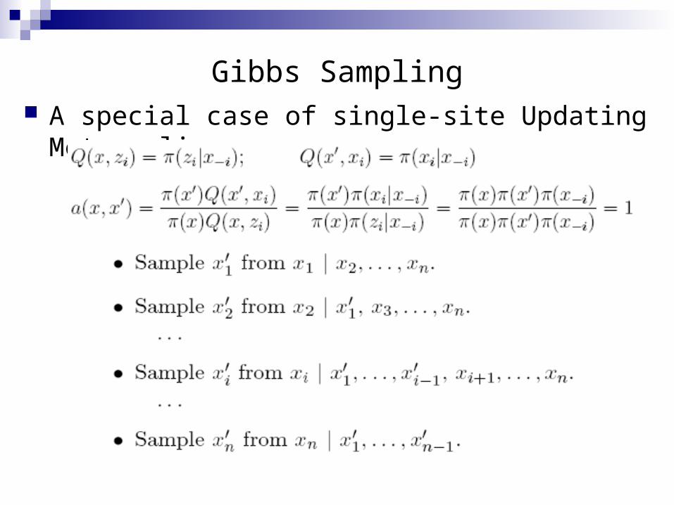
Gibbs Sampling A special case of single-site Updating Me-

tropolis

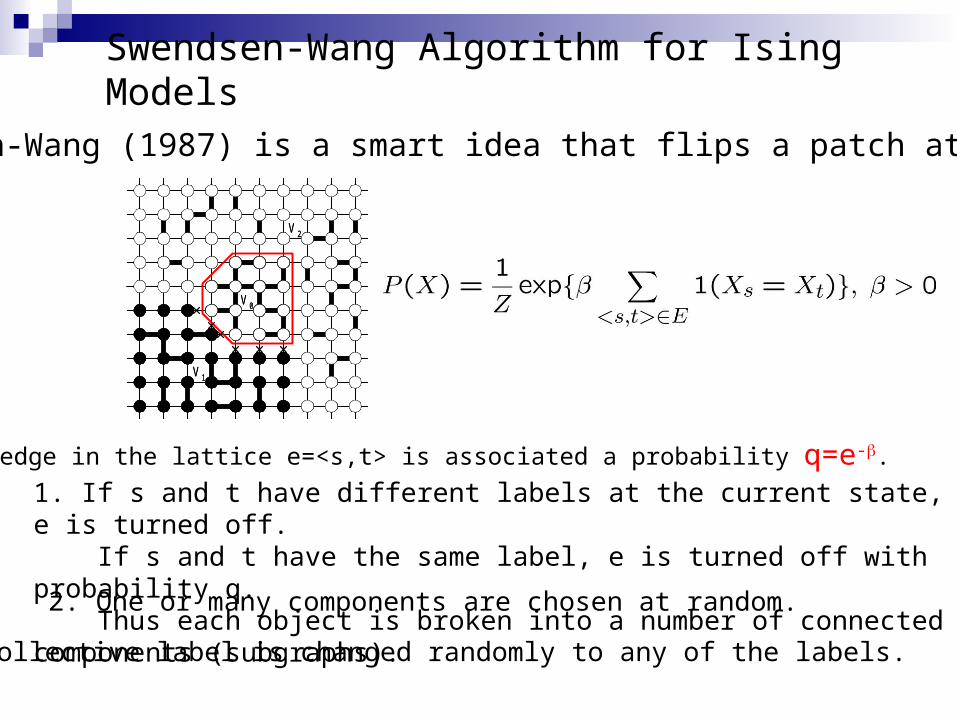
Swendsen-Wang Algorithm for Ising Models

Swedsen-Wang (1987) is a smart idea that flips a patch at a time.

Each edge in the lattice e=<s,t> is associated a probability q=e-b.

1. If s and t have different labels at the current state, e is turned off. If s and t have the same label, e is turned off with probability q. Thus each object is broken into a number of connected components (subgraphs). 2. One or many components are chosen at random.

V 0

V 2

V 1

3. The collective label is changed randomly to any of the labels.

V 0

V 2

V 1

Swendsen-Wang Algorithm

Pros: Computationally efficient in sampling the Ising

models Cons:

Limited to Ising models Not informed by data, slows down in the pres-

ence of an external field (data term)

Cf) Swendsen Wang Cuts Generalizes Swendsen-Wang to arbitrary posterior probabilities

Improves the clustering step by using the image data