Lecture 1 -Mathematical Preliminaries · Lecture 1 -Mathematical Preliminaries The Space Rn I Rn -...
39
Lecture 1 -Mathematical Preliminaries The Space R n I R n - the set of n-dimensional column vectors with real components endowed with the component-wise addition operator: x 1 x 2 . . . x n + y 1 y 2 . . . y n = x 1 + y 1 x 2 + y 2 . . . x n + y n , and the scalar-vector product λ x 1 x 2 . . . x n = λx 1 λx 2 . . . λx n , I e 1 , e 2 ,..., e n - standard/canonical basis. I e and 0 - all ones and all zeros column vectors. Amir Beck “Introduction to Nonlinear Optimization” Lecture Slides - Mathematical Preliminaries 1 / 24
Transcript of Lecture 1 -Mathematical Preliminaries · Lecture 1 -Mathematical Preliminaries The Space Rn I Rn -...
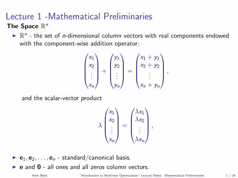
Lecture 1 -Mathematical PreliminariesThe Space Rn
I Rn - the set of n-dimensional column vectors with real components endowedwith the component-wise addition operator:
x1x2...xn
+
y1y2...yn
=
x1 + y1x2 + y2
...xn + yn
,
and the scalar-vector product
λ
x1x2...xn
=
λx1λx2
...λxn
,
I e1, e2, . . . , en - standard/canonical basis.
I e and 0 - all ones and all zeros column vectors.Amir Beck “Introduction to Nonlinear Optimization” Lecture Slides - Mathematical Preliminaries 1 / 24
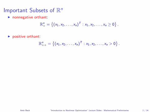
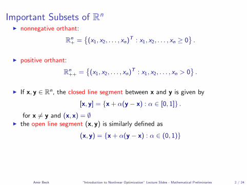
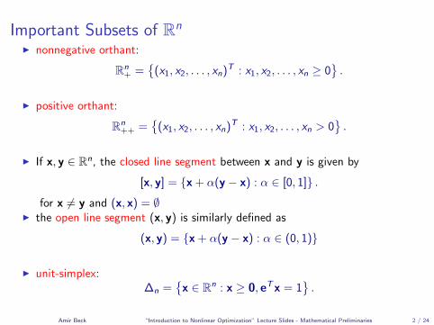
Important Subsets of Rn
I nonnegative orthant:
Rn+ =
{(x1, x2, . . . , xn)T : x1, x2, . . . , xn ≥ 0
}.
I positive orthant:
Rn++ =
{(x1, x2, . . . , xn)T : x1, x2, . . . , xn > 0
}.
I If x, y ∈ Rn, the closed line segment between x and y is given by
[x, y] = {x + α(y − x) : α ∈ [0, 1]} .
for x 6= y and (x, x) = ∅I the open line segment (x, y) is similarly defined as
(x, y) = {x + α(y − x) : α ∈ (0, 1)}
I unit-simplex:∆n =
{x ∈ Rn : x ≥ 0, eTx = 1
}.
Amir Beck “Introduction to Nonlinear Optimization” Lecture Slides - Mathematical Preliminaries 2 / 24
The Space Rm×n
I The set of all real valued matrices is denoted by Rm×n.
I In - n × n identity matrix.
I 0m×n - m × n zeros matrix.
Amir Beck “Introduction to Nonlinear Optimization” Lecture Slides - Mathematical Preliminaries 3 / 24
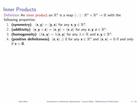
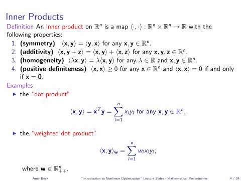
Inner ProductsDefinition An inner product on Rn is a map 〈·, ·〉 : Rn × Rn → R with thefollowing properties:
1. (symmetry) 〈x, y〉 = 〈y, x〉 for any x, y ∈ Rn.
2. (additivity) 〈x, y + z〉 = 〈x, y〉+ 〈x, z〉 for any x, y, z ∈ Rn.
3. (homogeneity) 〈λx, y〉 = λ〈x, y〉 for any λ ∈ R and x, y ∈ Rn.
4. (positive definiteness) 〈x, x〉 ≥ 0 for any x ∈ Rn and 〈x, x〉 = 0 if and onlyif x = 0.
ExamplesI the “dot product”
〈x, y〉 = xTy =n∑
i=1
xiyi for any x, y ∈ Rn.
I the “weighted dot product”
〈x, y〉w =n∑
i=1
wixiyi ,
where w ∈ Rn++.
Amir Beck “Introduction to Nonlinear Optimization” Lecture Slides - Mathematical Preliminaries 4 / 24
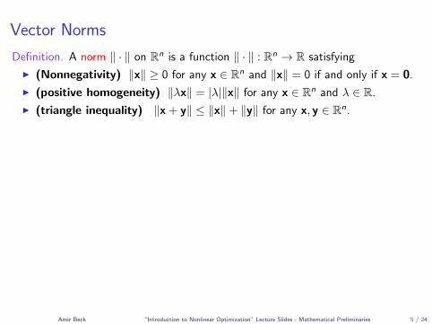
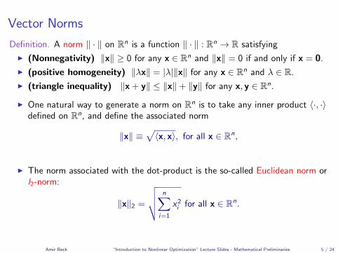
Vector Norms
Definition. A norm ‖ · ‖ on Rn is a function ‖ · ‖ : Rn → R satisfying
I (Nonnegativity) ‖x‖ ≥ 0 for any x ∈ Rn and ‖x‖ = 0 if and only if x = 0.
I (positive homogeneity) ‖λx‖ = |λ|‖x‖ for any x ∈ Rn and λ ∈ R.
I (triangle inequality) ‖x + y‖ ≤ ‖x‖+ ‖y‖ for any x, y ∈ Rn.
I One natural way to generate a norm on Rn is to take any inner product 〈·, ·〉defined on Rn, and define the associated norm
‖x‖ ≡√〈x, x〉, for all x ∈ Rn,
I The norm associated with the dot-product is the so-called Euclidean norm orl2-norm:
‖x‖2 =
√√√√ n∑i=1
x2i for all x ∈ Rn.
Amir Beck “Introduction to Nonlinear Optimization” Lecture Slides - Mathematical Preliminaries 5 / 24
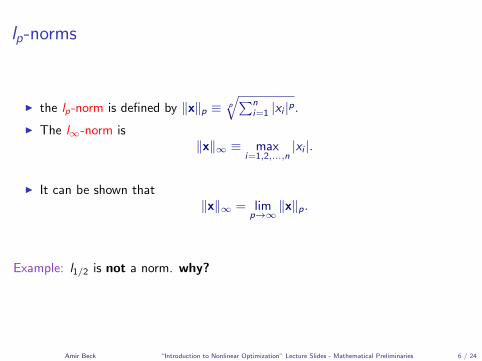
lp-norms
I the lp-norm is defined by ‖x‖p ≡ p
√∑ni=1 |xi |p.
I The l∞-norm is‖x‖∞ ≡ max
i=1,2,...,n|xi |.
I It can be shown that‖x‖∞ = lim
p→∞‖x‖p.
Example: l1/2 is not a norm. why?
Amir Beck “Introduction to Nonlinear Optimization” Lecture Slides - Mathematical Preliminaries 6 / 24
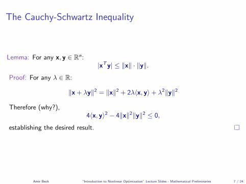
The Cauchy-Schwartz Inequality
Lemma: For any x, y ∈ Rn:|xTy| ≤ ‖x‖ · ‖y‖.
Proof: For any λ ∈ R:
‖x + λy‖2 = ‖x‖2 + 2λ〈x, y〉+ λ2‖y‖2
Therefore (why?),4〈x, y〉2 − 4‖x‖2‖y‖2 ≤ 0,
establishing the desired result.
Amir Beck “Introduction to Nonlinear Optimization” Lecture Slides - Mathematical Preliminaries 7 / 24
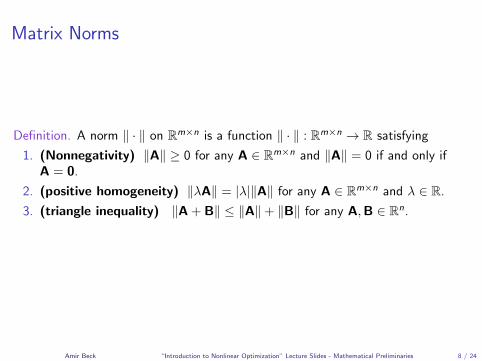
Matrix Norms
Definition. A norm ‖ · ‖ on Rm×n is a function ‖ · ‖ : Rm×n → R satisfying
1. (Nonnegativity) ‖A‖ ≥ 0 for any A ∈ Rm×n and ‖A‖ = 0 if and only ifA = 0.
2. (positive homogeneity) ‖λA‖ = |λ|‖A‖ for any A ∈ Rm×n and λ ∈ R.
3. (triangle inequality) ‖A + B‖ ≤ ‖A‖+ ‖B‖ for any A,B ∈ Rn.
Amir Beck “Introduction to Nonlinear Optimization” Lecture Slides - Mathematical Preliminaries 8 / 24
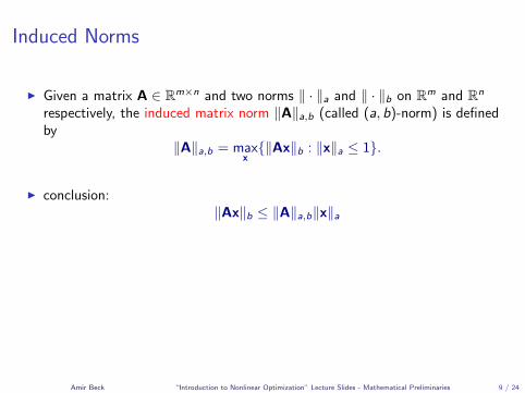
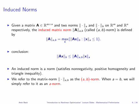
Induced Norms
I Given a matrix A ∈ Rm×n and two norms ‖ · ‖a and ‖ · ‖b on Rm and Rn
respectively, the induced matrix norm ‖A‖a,b (called (a, b)-norm) is definedby
‖A‖a,b = maxx{‖Ax‖b : ‖x‖a ≤ 1}.
I conclusion:‖Ax‖b ≤ ‖A‖a,b‖x‖a
I An induced norm is a norm (satisfies nonnegativity, positive homogeneity andtriangle inequality).
I We refer to the matrix-norm ‖ · ‖a,b as the (a, b)-norm. When a = b, we willsimply refer to it as an a-norm.
Amir Beck “Introduction to Nonlinear Optimization” Lecture Slides - Mathematical Preliminaries 9 / 24
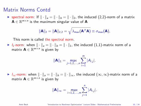
Matrix Norms ContdI spectral norm: If ‖ · ‖a = ‖ · ‖b = ‖ · ‖2, the induced (2,2)-norm of a matrix
A ∈ Rm×n is the maximum singular value of A
‖A‖2 = ‖A‖2,2 =√λmax(ATA) ≡ σmax(A),
This norm is called the spectral norm.
I l1-norm: when ‖ · ‖a = ‖ · ‖b = ‖ · ‖1, the induced (1,1)-matrix norm of amatrix A ∈ Rm×n is given by
‖A‖1 = maxj=1,2,...,n
m∑i=1
|Ai,j |.
I l∞-norm: when ‖ · ‖a = ‖ · ‖b = ‖ · ‖∞, the induced (∞,∞)-matrix norm of amatrix A ∈ Rm×n is given by
‖A‖∞ = maxi=1,2,...,m
n∑j=1
|Ai,j |.
Amir Beck “Introduction to Nonlinear Optimization” Lecture Slides - Mathematical Preliminaries 10 / 24
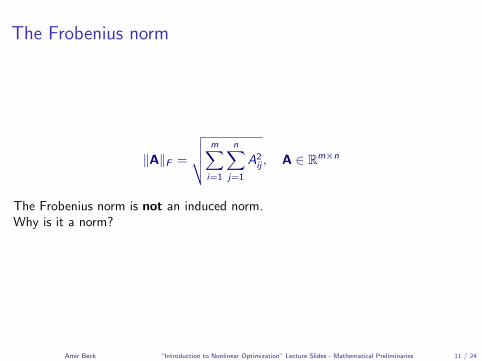
The Frobenius norm
‖A‖F =
√√√√ m∑i=1
n∑j=1
A2ij , A ∈ Rm×n
The Frobenius norm is not an induced norm.Why is it a norm?
Amir Beck “Introduction to Nonlinear Optimization” Lecture Slides - Mathematical Preliminaries 11 / 24
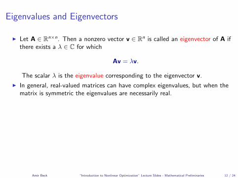
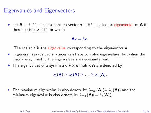
Eigenvalues and Eigenvectors
I Let A ∈ Rn×n. Then a nonzero vector v ∈ Rn is called an eigenvector of A ifthere exists a λ ∈ C for which
Av = λv.
The scalar λ is the eigenvalue corresponding to the eigenvector v.
I In general, real-valued matrices can have complex eigenvalues, but when thematrix is symmetric the eigenvalues are necessarily real.
I The eigenvalues of a symmetric n × n matrix A are denoted by
λ1(A) ≥ λ2(A) ≥ . . . ≥ λn(A).
I The maximum eigenvalue is also denote by λmax(A)(= λ1(A)) and theminimum eigenvalue is also denote by λmin(A)(= λn(A)).
Amir Beck “Introduction to Nonlinear Optimization” Lecture Slides - Mathematical Preliminaries 12 / 24
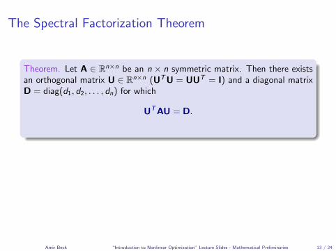
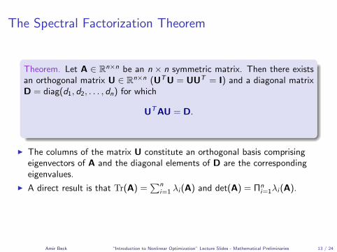
The Spectral Factorization Theorem
Theorem. Let A ∈ Rn×n be an n × n symmetric matrix. Then there existsan orthogonal matrix U ∈ Rn×n (UTU = UUT = I) and a diagonal matrixD = diag(d1, d2, . . . , dn) for which
UTAU = D.
I The columns of the matrix U constitute an orthogonal basis comprisingeigenvectors of A and the diagonal elements of D are the correspondingeigenvalues.
I A direct result is that Tr(A) =∑n
i=1 λi (A) and det(A) = Πni=1λi (A).
Amir Beck “Introduction to Nonlinear Optimization” Lecture Slides - Mathematical Preliminaries 13 / 24
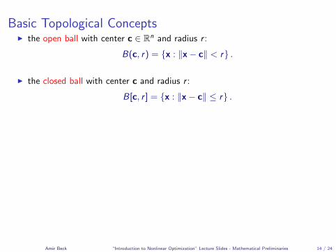
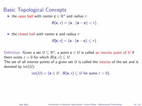
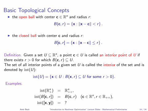
Basic Topological ConceptsI the open ball with center c ∈ Rn and radius r :
B(c, r) = {x : ‖x− c‖ < r} .
I the closed ball with center c and radius r :
B[c, r ] = {x : ‖x− c‖ ≤ r} .
Definition. Given a set U ⊆ Rn, a point c ∈ U is called an interior point of U ifthere exists r > 0 for which B(c, r) ⊆ U.The set of all interior points of a given set U is called the interior of the set and isdenoted by int(U):
int(U) = {x ∈ U : B(x, r) ⊆ U for some r > 0}.Examples.
int(Rn+) = Rn
++,
int(B[c, r ]) = B(c, r) (c ∈ Rn, r ∈ R++),
int([x, y]) = ?
Amir Beck “Introduction to Nonlinear Optimization” Lecture Slides - Mathematical Preliminaries 14 / 24
Basic Topological ConceptsI the open ball with center c ∈ Rn and radius r :
B(c, r) = {x : ‖x− c‖ < r} .
I the closed ball with center c and radius r :
B[c, r ] = {x : ‖x− c‖ ≤ r} .
Definition. Given a set U ⊆ Rn, a point c ∈ U is called an interior point of U ifthere exists r > 0 for which B(c, r) ⊆ U.The set of all interior points of a given set U is called the interior of the set and isdenoted by int(U):
int(U) = {x ∈ U : B(x, r) ⊆ U for some r > 0}.
Examples.
int(Rn+) = Rn
++,
int(B[c, r ]) = B(c, r) (c ∈ Rn, r ∈ R++),
int([x, y]) = ?
Amir Beck “Introduction to Nonlinear Optimization” Lecture Slides - Mathematical Preliminaries 14 / 24
Basic Topological ConceptsI the open ball with center c ∈ Rn and radius r :
B(c, r) = {x : ‖x− c‖ < r} .
I the closed ball with center c and radius r :
B[c, r ] = {x : ‖x− c‖ ≤ r} .
Definition. Given a set U ⊆ Rn, a point c ∈ U is called an interior point of U ifthere exists r > 0 for which B(c, r) ⊆ U.The set of all interior points of a given set U is called the interior of the set and isdenoted by int(U):
int(U) = {x ∈ U : B(x, r) ⊆ U for some r > 0}.Examples.
int(Rn+) = Rn
++,
int(B[c, r ]) = B(c, r) (c ∈ Rn, r ∈ R++),
int([x, y]) = ?
Amir Beck “Introduction to Nonlinear Optimization” Lecture Slides - Mathematical Preliminaries 14 / 24
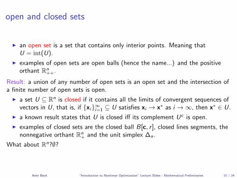
open and closed sets
I an open set is a set that contains only interior points. Meaning thatU = int(U).
I examples of open sets are open balls (hence the name...) and the positiveorthant Rn
++.
Result: a union of any number of open sets is an open set and the intersection ofa finite number of open sets is open.
I a set U ⊆ Rn is closed if it contains all the limits of convergent sequences ofvectors in U, that is, if {xi}∞i=1 ⊆ U satisfies xi → x∗ as i →∞, then x∗ ∈ U.
I a known result states that U is closed iff its complement Uc is open.
I examples of closed sets are the closed ball B[c, r ], closed lines segments, thenonnegative orthant Rn
+ and the unit simplex ∆n.
What about Rn?∅?
Amir Beck “Introduction to Nonlinear Optimization” Lecture Slides - Mathematical Preliminaries 15 / 24
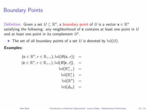
Boundary Points
Definition. Given a set U ⊆ Rn, a boundary point of U is a vector x ∈ Rn
satisfying the following: any neighborhood of x contains at least one point in Uand at least one point in its complement Uc .
I The set of all boundary points of a set U is denoted by bd(U).
Examples:
(c ∈ Rn, r ∈ R++),bd(B(c, r)) = ksjdhfsdkfjhsdfkjhsdfkjh
(c ∈ Rn, r ∈ R++),bd(B[c, r ]), =
bd(Rn++) =
bd(Rn+) =
bd(Rn) =
bd(∆n) =
Amir Beck “Introduction to Nonlinear Optimization” Lecture Slides - Mathematical Preliminaries 16 / 24
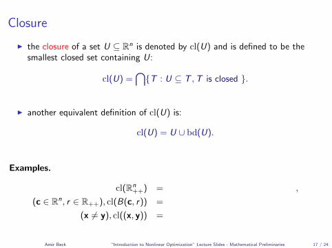
Closure
I the closure of a set U ⊆ Rn is denoted by cl(U) and is defined to be thesmallest closed set containing U:
cl(U) =⋂{T : U ⊆ T ,T is closed }.
I another equivalent definition of cl(U) is:
cl(U) = U ∪ bd(U).
Examples.
cl(Rn++) = ksjdhfksdfkjhsdfkjhdsfsdkfjhsdkf ,
(c ∈ Rn, r ∈ R++), cl(B(c, r)) =
(x 6= y), cl((x, y)) =
Amir Beck “Introduction to Nonlinear Optimization” Lecture Slides - Mathematical Preliminaries 17 / 24
Boundedness and Compactness
I A set U ⊆ Rn is called bounded if there exists M > 0 for which U ⊆ B(0,M).
I A set U ⊆ Rn is called compact if it is closed and bounded.
I Examples of compact sets: closed balls, unit simplex, closed line segments.
Amir Beck “Introduction to Nonlinear Optimization” Lecture Slides - Mathematical Preliminaries 18 / 24
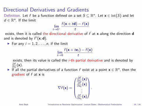
Directional Derivatives and GradientsDefinition. Let f be a function defined on a set S ⊆ Rn. Let x ∈ int(S) and letd ∈ Rn. If the limit
limt→0+
f (x + td)− f (x)
texists, then it is called the directional derivative of f at x along the direction d
and is denoted by f ′(x; d).I For any i = 1, 2, . . . , n, if the limit
limt→0
f (x + tei )− f (x)
t
exists, then its value is called the i-th partial derivative and is denoted by∂f∂xi
(x).I If all the partial derivatives of a function f exist at a point x ∈ Rn, then the
gradient of f at x is
∇f (x) =
∂f∂x1
(x)∂f∂x2
(x)...
∂f∂xn
(x)
.
Amir Beck “Introduction to Nonlinear Optimization” Lecture Slides - Mathematical Preliminaries 19 / 24
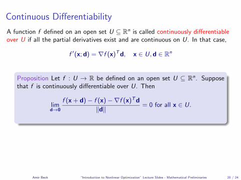
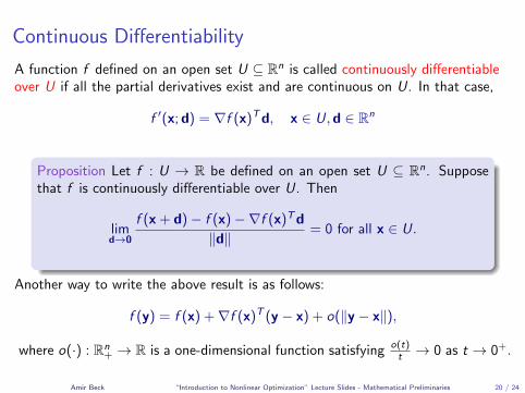
Continuous Differentiability
A function f defined on an open set U ⊆ Rn is called continuously differentiableover U if all the partial derivatives exist and are continuous on U. In that case,
f ′(x; d) = ∇f (x)Td, x ∈ U,d ∈ Rn
Proposition Let f : U → R be defined on an open set U ⊆ Rn. Supposethat f is continuously differentiable over U. Then
limd→0
f (x + d)− f (x)−∇f (x)Td
‖d‖= 0 for all x ∈ U.
Another way to write the above result is as follows:
f (y) = f (x) +∇f (x)T (y − x) + o(‖y − x‖),
where o(·) : Rn+ → R is a one-dimensional function satisfying o(t)
t → 0 as t → 0+.
Amir Beck “Introduction to Nonlinear Optimization” Lecture Slides - Mathematical Preliminaries 20 / 24
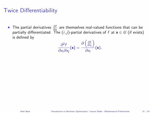
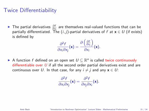
Twice Differentiability
I The partial derivatives ∂f∂xi
are themselves real-valued functions that can bepartially differentiated. The (i , j)-partial derivatives of f at x ∈ U (if exists)is defined by
∂2f
∂xi∂xj(x) =
∂(
∂f∂xj
)∂xi
(x).
I A function f defined on an open set U ⊆ Rn is called twice continuouslydifferentiable over U if all the second order partial derivatives exist and arecontinuous over U. In that case, for any i 6= j and any x ∈ U:
∂2f
∂xi∂xj(x) =
∂2f
∂xj∂xi(x).
Amir Beck “Introduction to Nonlinear Optimization” Lecture Slides - Mathematical Preliminaries 21 / 24
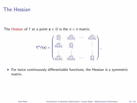
The Hessian
The Hessian of f at a point x ∈ U is the n × n matrix:
∇2f (x) =
∂2f∂x21
∂2f∂x1∂x2
· · · ∂2f∂x1∂xn
∂2f∂x2∂x1
∂2f∂x22
...
......
...∂2f
∂xn∂x1
∂2f∂xn∂x2
· · · ∂2f∂x2n
,
I For twice continuously differentiable functions, the Hessian is a symmetricmatrix.
Amir Beck “Introduction to Nonlinear Optimization” Lecture Slides - Mathematical Preliminaries 22 / 24
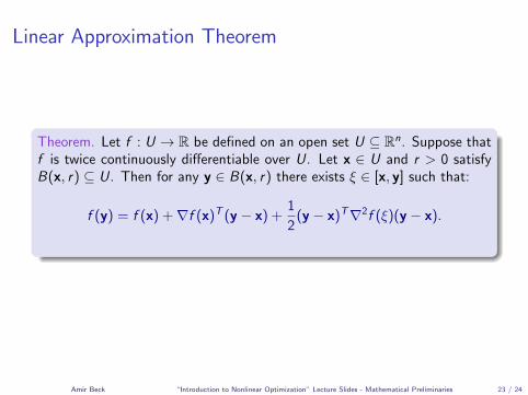
Linear Approximation Theorem
Theorem. Let f : U → R be defined on an open set U ⊆ Rn. Suppose thatf is twice continuously differentiable over U. Let x ∈ U and r > 0 satisfyB(x, r) ⊆ U. Then for any y ∈ B(x, r) there exists ξ ∈ [x, y] such that:
f (y) = f (x) +∇f (x)T (y − x) +1
2(y − x)T∇2f (ξ)(y − x).
Amir Beck “Introduction to Nonlinear Optimization” Lecture Slides - Mathematical Preliminaries 23 / 24
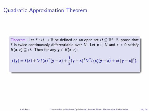
Quadratic Approximation Theorem
Theorem. Let f : U → R be defined on an open set U ⊆ Rn. Suppose thatf is twice continuously differentiable over U. Let x ∈ U and r > 0 satisfyB(x, r) ⊆ U. Then for any y ∈ B(x, r):
f (y) = f (x) +∇f (x)T (y − x) +1
2(y − x)T∇2f (x)(y − x) + o(‖y − x‖2).
Amir Beck “Introduction to Nonlinear Optimization” Lecture Slides - Mathematical Preliminaries 24 / 24