L R I

SEMI-PERSISTENT DATA STRUCTURES

CONCHON S / FILLIATRE J C

Unité Mixte de Recherche 8623 CNRS-Université Paris Sud – LRI

09/2007

Rapport de Recherche N° 1474

CNRS – Université de Paris Sud Centre d’Orsay

LABORATOIRE DE RECHERCHE EN INFORMATIQUE Bâtiment 490

91405 ORSAY Cedex (France)

Semi-Persistent Data Structures

Sylvain Conchon and Jean-Christophe FilliatreLRI, Univ Paris-Sud, CNRS, Orsay F-91405

INRIA Futurs, ProVal, Parc Orsay Universite, F-91893{conchon,filliatr}@lri.fr

September 21, 2007

Abstract

A data structure is said to be persistent when any update operation returnsa new structure without altering the old version. This paper introduces a newnotion of persistence, called semi-persistence, where only ancestors of the most re-cent version can be accessed or updated. Making a data structure semi-persistentmay improve its time and space complexity. This is of particular interest in back-tracking algorithms manipulating persistent data structures, where this propertyis usually satisfied. We propose a proof system to statically check the valid use ofsemi-persistent data structures. It requires a few annotations from the user andthen generates proof obligations that are automatically discharged by a dedicateddecision procedure. Additionally, we give some examples of semi-persistent datastructures (arrays, lists and hash tables).

1 Introduction

A data structure is said to be persistent when any update operation returns a newstructure without altering the old version. In purely applicative programming, datastructures are automatically persistent [15]. Yet this notion is more general and theexact meaning of persistent is observationally immutable. Driscoll et al. even proposedsystematic techniques to make imperative data structures persistent [7]. In particular,they distinguish partial persistence, where all versions can be accessed but only the newestcan be updated, from full persistence where any version can be accessed or updated. Inthis paper, we study another notion of persistence, which we call semi-persistence.

One of the main interests of a persistent data structure shows up when it is usedwithin a backtracking algorithm. Indeed, when we are back from a branch, there is noneed to undo the modifications performed on the data structure: we simply use the oldversion, which persisted, and start a new branch. One can immediately notice that fullpersistence is not needed in this case, since we are reusing ancestors of the current version,but never siblings (in the sense of another version obtained from a common ancestor).We shall call semi-persistent a data structure where only ancestors of the newest versioncan be updated. Note that this notion is different from partial persistence, since we needto update ancestors, and not only to access them.

1

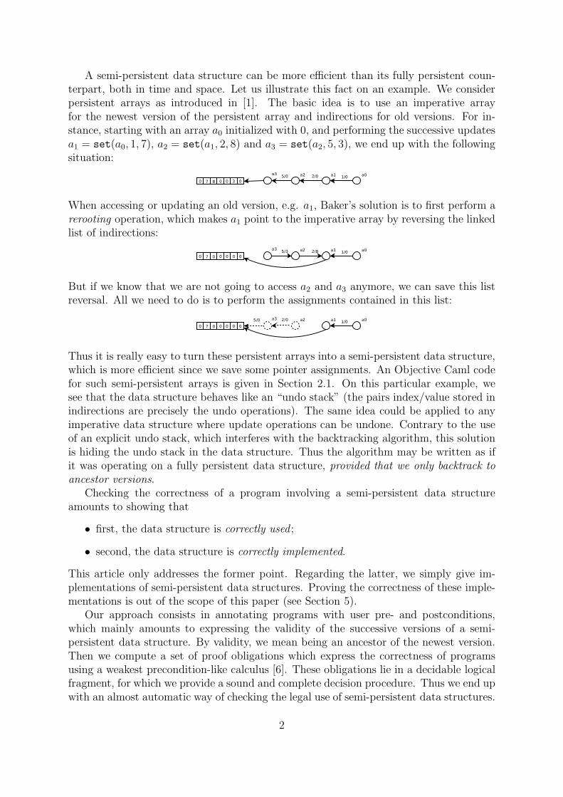
A semi-persistent data structure can be more efficient than its fully persistent coun-terpart, both in time and space. Let us illustrate this fact on an example. We considerpersistent arrays as introduced in [1]. The basic idea is to use an imperative arrayfor the newest version of the persistent array and indirections for old versions. For in-stance, starting with an array a0 initialized with 0, and performing the successive updatesa1 = set(a0, 1, 7), a2 = set(a1, 2, 8) and a3 = set(a2, 5, 3), we end up with the followingsituation:

When accessing or updating an old version, e.g. a1, Baker’s solution is to first perform arerooting operation, which makes a1 point to the imperative array by reversing the linkedlist of indirections:

But if we know that we are not going to access a2 and a3 anymore, we can save this listreversal. All we need to do is to perform the assignments contained in this list:

Thus it is really easy to turn these persistent arrays into a semi-persistent data structure,which is more efficient since we save some pointer assignments. An Objective Caml codefor such semi-persistent arrays is given in Section 2.1. On this particular example, wesee that the data structure behaves like an “undo stack” (the pairs index/value stored inindirections are precisely the undo operations). The same idea could be applied to anyimperative data structure where update operations can be undone. Contrary to the useof an explicit undo stack, which interferes with the backtracking algorithm, this solutionis hiding the undo stack in the data structure. Thus the algorithm may be written as ifit was operating on a fully persistent data structure, provided that we only backtrack toancestor versions.

Checking the correctness of a program involving a semi-persistent data structureamounts to showing that

• first, the data structure is correctly used ;

• second, the data structure is correctly implemented.

This article only addresses the former point. Regarding the latter, we simply give im-plementations of semi-persistent data structures. Proving the correctness of these imple-mentations is out of the scope of this paper (see Section 5).

Our approach consists in annotating programs with user pre- and postconditions,which mainly amounts to expressing the validity of the successive versions of a semi-persistent data structure. By validity, we mean being an ancestor of the newest version.Then we compute a set of proof obligations which express the correctness of programsusing a weakest precondition-like calculus [6]. These obligations lie in a decidable logicalfragment, for which we provide a sound and complete decision procedure. Thus we end upwith an almost automatic way of checking the legal use of semi-persistent data structures.

2

To make it more precise, let us consider two programs manipulating a semi-persistentdata structure. Each program is a function taking a version x0 of the data structure asargument, generating new versions using an update operation upd and finally accessingthe resulting version using an access operation acc :

fun f x0 ={valid(x0)}let x1 = upd x0 in

let x2 = upd x0 in

acc x2

fun g x0 ={valid(x0)}let x1 = upd x0 in

let x2 = upd x0 in

acc x1

Each function has a precondition requiring the validity of x0 (through a valid predicate).Then both functions successively build two new versions x1 and x2 as successors of x0.This can be illustrated by the following version trees, where arrows represent versionsuccessors and a dashed arrow stands for a version that has become invalid:

Finally, function f accesses x2, which is legal; and function g accesses x1, which is illegalsince x1 is not an ancestor of the newest version x2. If the xi were semi-persistent arrays,as described above, the contents of x1 would indeed be modified by the creation of x2.Thus x1 should not be accessed anymore.

As illustrated by this example, evaluation order matters as the creation of a newversion has side-effects on other versions. Thus semi-persistence is clearly related toimpure data structures. For this reason, our weakest precondition calculus relies on asmall effect inference which detects the mutation of the data structure.

Related work. To our knowledge, this notion of semi-persistence is new. However,there are several domains which are somehow connected to our work, either because theyare related to some kind of stack analysis, or because they are providing decision proce-dure for reachability issues. First, works on escape analysis [10, 4] address the problem ofstack-allocating values; we may think that semi-persistent versions that become invalidare precisely those which could be stack-allocated, but it is not the case as illustrated byexample g above. Second, works on stack analysis to ensure memory safety [13, 17, 18]provide methods to check the consistent use of push and pop operations. However, theseapproaches are not precise enough to distinguish between two sibling versions (of a givensemi-persistent data structure) which are both upper in the stack. Regarding the decid-ability of our proof obligations, our approach is similar to other works regarding reach-ability in linked data structures [14, 3, 16]. However, our logic is much simpler and weprovide a specific decision procedure. Finally, we can mention Knuth’s dancing links [11]as an example of a data structure specifically designed for backtracking algorithms; butit is still a traditional imperative solution where an explicit undo operation is performedin the main algorithm.

This paper is organized as follows. First, Section 2 gives examples of semi-persistentdata structures and shows the benefits of semi-persistence with some benchmarks. Then

3

our formalization of semi-persistence is presented in two steps: Section 3 introduces asmall programming language to manipulate semi-persistent data structures, and Section 4defines the proof system which checks the valid use of semi-persistent data structures.Section 5 concludes with possible extensions.

2 Examples of Semi-Persistent Data Structures

We present the implementation of semi-persistent arrays, lists and hash tables and bench-marks to show the benefits of semi-persistence. All these examples are written in Objec-tive Caml [12].

2.1 Arrays

First we implement semi-persistent arrays, as described in the introduction of this paper.The interface is similar to persistent arrays:

type α t

val create : int → α → α t

val get : α t → int → α

val set : α t → int → α → α t

Type α t is the polymorphic type of semi-persistent arrays containing values of type α.create n v creates a new array of size n with all cells initialized with v. get and set arethe usual access and update functions.

A semi-persistent array is a reference containing a value of type α data, which iseither an imperative array from Ocaml’s standard library or an indirection:

type α t = α data ref

and α data =

| Newest of α array

| Diff of int × α × α t

Newest a stands for the newest version of the structure, and Diff (i, v, a) stands for asemi-persistent array sharing the contents of a, except at index i where its value is v.

Creation of a new semi-persistent array is simply an allocation of a new referencecontaining a new imperative array:

let create n v = ref (Newest (Array.create n v))

To implement get and set, we first need to implement the rerooting operation de-scribed in the introduction, which backtracks to a given version. In this semi-persistentimplementation, it simply amounts to writing the values in Diff nodes into the imperativearray:

let rec reroot t = match !t with

| Newest →()

| Diff (i, v, t’) →

4

reroot t’;

let Newest a as n = !t’ in

a.(i) ← v;

t := n

A call reroot t ensures that t is now the newest version (and thus a direct access to theimperative array); hence we can safely match !t’ against the Newest constructor afterthe recursive call. Note that reroot could be written in CPS to avoid a possible stackoverflow.

Then both get and set start with a call to reroot and thus safely ignore the case ofan indirection:

let get t i =

reroot t;

let Newest a = !t in a.(i)

let set t i v =

reroot t;

let Newest a as n = !t in

let old = a.(i) in

a.(i) ← v;

let res = ref n in

t := Diff (i, old, res);

res

The only difference with the fully persistent implementation is in function reroot, wherethe sequence a.(i) ← v; t := n would be replaced by the more complex code:

let v’ = a.(i) in

a.(i) ← v;

t := n;

t’ := Diff (i, v’, t)

Thus we save, in the semi-persistent implementation, an array access, a constructorallocation and an assignment.

It is worth noticing that get performs a reroot operation only to improve furthercalls to get and set. This is definitely the good choice in a pure backtracking algorithm(i.e. where we only access the current version or backtrack to some previous version).But we could imagine a more complex algorithm where we need to access to previousversions without backtracking. For this purpose, we could also provide a non-destructiveaccess operation, nd get, which simply follows the Diff stack:

let rec nd_get t i = match !t with

| Newest a →a.(i)

| Diff (j, v, t’) →if i = j then v else nd_get t’ i

Our formalization of semi-persistence will handle both kinds of access operations.

5

2.2 Lists

As a second example, we consider an immutable data structure which we make semi-persistent. The simplest and most popular example is the list data structure. To makeit semi-persistent, the idea is to reuse cons cells between successive conses to the samelist. For instance, given a list l, the cons operation 1::l allocates a new memory blockto store 1 and a pointer to l. Then a successive operation 2::l could reuse the samememory block if the list is used in a semi-persistent way. Thus we simply need to replace1 by 2. To do this, we must maintain for each list the previous cons, if any.

To implement semi-persistent lists, we use the following type of double-linked lists:

type α t = { mutable head : α;

tail : α t;

mutable pc : α t }

Fields head and tail are the usual fields for linked lists, except that head is a mutablefield to allow further modification of its contents. The additional field pc keeps track ofa previous cons, if any.

Similarly to the constant null in C or Java programs, we would like to represent theempty list as a statically allocated constant value of type α t. Since there is no wayto build such a polymorphic value (we can not instantiate the head field), we turn theempty list into a function taking a dummy value as argument:

let nil v =

let rec null =

{ head = v; tail = null; pc = null }in null

This function allocates a single cons cell null where tail and pc fields are physicallyequal to null. Thus testing for the empty list is as simple as

let is_nil l = l.tail == l

Additionally, the empty list is used as the value for pc when there is no previous cons.The cons function checks the existence of a previously allocated block (testing pc for

being the empty list) and reuses it if any:

let cons x l =

if is_nil l.pc then begin

let n = { l with head=x; tail=l } in

if not (is_nil l) then l.pc ← n;

n

end else begin

let c = l.pc in

c.head ← x;

c

end

The test not (is nil l) prevents from reusing the successor of the empty list, since itis shared by all lists.

Implementing the tail operation is immediate:

6

let tail l = l.tail

Though tail does not modify l, it makes it invalid since a subsequent cons on the resultof tail l would modify the head of l in place. Contrary to operation get on arrays,it is not possible to implement a non-destructive version of tail. Yet it is possible toprovide other, non-destructive, access operations, such as a membership test function:

let rec mem x l =

not (is_nil l) && (l.head = x || mem x l.tail)

It is worth noticing that these semi-persistent lists are trading off allocation for deal-location. Indeed, the average use of these lists requires less allocation than ordinaryimmutable lists (the cons cells are slightly bigger but are reusable). But, on the contrary,such lists prevent deallocation since a pointer p to a 1-element list cons x nil makes allsubsequent conses alive as long as p is alive.

Such semi-persistent lists could even be used to improve the implementation of semi-persistent arrays from the previous section, since Diff cells could similarly be reused.

2.3 Hash Tables

Combining (semi-)persistent arrays with (semi-)persistent lists, one easily gets (semi-)persistent hash tables. Such a combination is nicely implemented as a module param-eterized with data structures for arrays and lists respectively. Introducing the followingsignatures for these parameters:

module type Array = sig

type α t

val create : int → α → α t

val get : α t → int → α

val set : α t → int → α → α t

end

module type List = sig

type α t

val nil : α → α t

val cons : α → α t → α t

val mem : α → α t → bool

end

the generic implementation of hash tables is as follows:

module MakeHT(PA : Array)(IL : List) = struct

type α t = { size : int; data : α IL.t PA.t }

let create n v =

{ size = n; data = PA.create n (IL.nil v) }

let add h x =

let i = x mod h.size in

7

{ h with data =

PA.set h.data i

(IL.cons x (PA.get h.data i)) }

let mem h x =

let i = x mod h.size in

IL.mem x (PA.get h.data i)

end

By instantiating arrays and lists implementations by semi-persistent arrays and lists fromSections 2.1 and 2.2 respectively, we automatically get semi-persistent hash tables. Notethat mem is a non-destructive operation only if PA.get is.

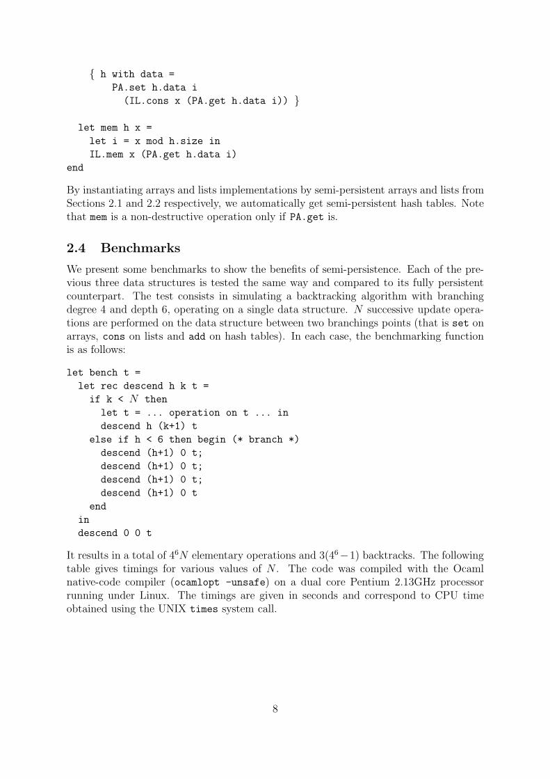
2.4 Benchmarks

We present some benchmarks to show the benefits of semi-persistence. Each of the pre-vious three data structures is tested the same way and compared to its fully persistentcounterpart. The test consists in simulating a backtracking algorithm with branchingdegree 4 and depth 6, operating on a single data structure. N successive update opera-tions are performed on the data structure between two branchings points (that is set onarrays, cons on lists and add on hash tables). In each case, the benchmarking functionis as follows:

let bench t =

let rec descend h k t =

if k < N then

let t = ... operation on t ... in

descend h (k+1) t

else if h < 6 then begin (* branch *)

descend (h+1) 0 t;

descend (h+1) 0 t;

descend (h+1) 0 t;

descend (h+1) 0 t

end

in

descend 0 0 t

It results in a total of 46N elementary operations and 3(46−1) backtracks. The followingtable gives timings for various values of N . The code was compiled with the Ocamlnative-code compiler (ocamlopt -unsafe) on a dual core Pentium 2.13GHz processorrunning under Linux. The timings are given in seconds and correspond to CPU timeobtained using the UNIX times system call.

8

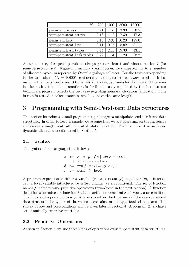
N 200 1000 5000 10000

persistent arrays 0.21 1.50 13.90 30.5semi-persistent arrays 0.18 1.10 7.59 17.3

persistent lists 0.18 2.38 50.20 195.0semi-persistent lists 0.11 0.76 8.02 31.1

persistent hash tables 0.24 2.15 19.30 43.1semi-persistent hash tables 0.22 1.51 11.20 28.2

As we can see, the speedup ratio is always greater than 1 and almost reaches 7 (forsemi-persistent lists). Regarding memory consumption, we compared the total numberof allocated bytes, as reported by Ocaml’s garbage collector. For the tests correspondingto the last column (N = 10000) semi-persistent data structures always used much lessmemory than persistent ones: 3 times less for arrays, 575 times less for lists and 1.5 timesless for hash tables. The dramatic ratio for lists is easily explained by the fact that ourbenchmark program reflects the best case regarding memory allocation (allocation in onebranch is reused in other branches, which all have the same length).

3 Programming with Semi-Persistent Data Structures

This section introduces a small programming language to manipulate semi-persistent datastructures. In order to keep it simple, we assume that we are operating on the successiveversions of a single, statically allocated, data structure. Multiple data structures anddynamic allocation are discussed in Section 5.

3.1 Syntax

The syntax of our language is as follows:

e ::= x | c | p | f e | let x = e in e

| if e then e else e

d ::= fun f (x : ι) = {φ} e {ψ}ι ::= semi | δ | bool

A program expression is either a variable (x), a constant (c), a pointer (p), a functioncall, a local variable introduced by a let binding, or a conditional. The set of functionnames f includes some primitive operations (introduced in the next section). A functiondefinition d introduces a function f with exactly one argument x of type ι, a preconditionφ, a body and a postcondition ψ. A type ι is either the type semi of the semi-persistentdata structure, the type δ of the values it contains, or the type bool of booleans. Thesyntax of pre- and postconditions will be given later in Section 4. A program ∆ is a finiteset of mutually recursive functions.

3.2 Primitive Operations

As seen in Section 2, we use three kinds of operations on semi-persistent data structures:

9

• update operations backtracking to a given version and creating a new successor,which becomes the newest version;

• destructive access operations backtracking to a given version, which becomes thenewest version, and then accessing it;

• non-destructive access operations accessing an ancestor of the newest version, with-out modifying the data structure.

Since update and destructive access operations both need to backtrack, it is convenientto design a language based on the following three primitives:

• backtrack: backtracks to a given version, making it the newest version;

• branch: builds a new successor of a given version, assuming it is the newest version;

• acc: accesses a given version, assuming it is a valid version.

Then update and destructive access operations can be rephrased in terms of the aboveprimitives:

upd e = branch (backtrack e)dacc e = acc (backtrack e)

3.3 Operational Semantics

We equip our language with a small step operational semantics, which is given in Figure 1.One step of reduction is written e1, S1 → e2, S2 where e1 and e2 are program expressionsand S1 and S2 are states. A value v is either a constant c or a pointer p. Pointers representversions of the semi-persistent data structure. A state S is a stack p1, . . . , pm of pointers,pm being the top of the stack. The semantics is straightforward, except for primitiveoperations. Primitive backtrack expects an argument pn designating a valid version ofthe data structure, that is an element of the stack. Then all pointers on top of pn arepopped from the stack and pn is the result of the operation. Primitive branch expectsan argument pn being the top of the stack and pushes a new value p, which is also theresult of the operation. Finally, primitive acc expects an argument pn designating a validversion, leaves the stack unchanged and returns some value for version pn, representedby A(pn). (We leave A uninterpreted since we are not interested in the values containedin the data structure.)

Note that reduction of backtrack pn or acc pn is blocked whenever pn is not anelement of S, which is precisely what we intend to prevent.

There is an obvious property of reduction which will be useful in Section 4.4:

Lemma 1 The first element of a state is preserved by reduction, that is if e, pS → e′, S ′

then S ′ = pS ′′.

10

E ::= [] | f E | let x = E in e | if E then e else e

v ::= c | pS ::= p · · ·p

if true then e1 else e2, S → e1, S

if false then e1 else e2, S → e2, S

let x = v in e, S → e{x← v}, Sf v, S → e{x← v}, S if fun f (x : ι) = {φ} e {ψ} ∈ ∆

backtrack pn, p1 · · · pnpn+1 · · ·pm → pn, p1 · · ·pn

branch pn, p1 · · · pn → p, p1 · · ·pnp p freshacc pn, p1 · · · pnpn+1 · · ·pm → A(pn), p1 · · · pnpn+1 · · · pm

E[e1], S1 → E[e2], S2 if e1, S1 → e2, S2 and E 6= []

Figure 1: Operational Semantics

3.4 Type System with Effect

We introduce a type system to characterize well-formed programs. Our language issimply typed and thus type-checking is immediate. Meanwhile, we infer the effect ǫof each expression, as an element of the boolean lattice ({⊥,⊤},∧,∨). This booleanindicates whether the expression modifies the semi-persistent data structure (⊥ meaningno modification and ⊤ a modification). Effects will be used in the next section to simplifyconstraint generation. Each function is given a type τ , as follows:

τ ::= (x : ι)→ǫ {φ} ι {ψ}

The argument is given a type and a name (x) since it is bound in both precondition φ

and postcondition ψ. Type τ also indicates the latent effect ǫ of the function, which isthe effect resulting from the function application.

A typing environment Γ is a set of type assignments for variables (x : ι), constants(c : ι) and functions (f : τ). It is assumed to contain at least type declarations for theprimitives, as follows:

backtrack : (x : semi)→⊤ {φbacktrack} semi {ψbacktrack}branch : (x : semi)→⊤ {φbranch} semi {ψbranch}

acc : (x : semi)→⊥ {φacc} δ {ψacc}

where pre- and postcondition are given later. As expected, both backtrack and branch

modify the semi-persistent data structure and thus have effect⊤, while the non-destructiveaccess acc has effect ⊥.

Given a typing environment Γ, the judgment Γ ⊢ e : ι, ǫ means “e is a well-formedexpression of type ι and effect ǫ” and the judgment Γ ⊢ d : τ means “d is a well-formedfunction definition of type τ”. Typing rules are given in Figure 2. They assume judgmentsΓ ⊢ φ pre and Γ ⊢ ψ post ι for the well-formedness of pre- and postconditions respectively,to be defined later in Section 4.1. Note that there is no typing rule for pointers, to preventtheir explicit use in programs.

11

Varx : ι ∈ Γ

Γ ⊢ x : ι,⊥Const

c : ι ∈ Γ

Γ ⊢ c : ι,⊥

Appf : (x : ι1)→

ǫ2 {φ} ι2 {ψ} ∈ Γ Γ ⊢ e : ι1, ǫ1

Γ ⊢ f e : ι2, ǫ1 ∨ ǫ2

IteΓ ⊢ e1 : bool, ǫ1 Γ ⊢ e2 : ι, ǫ2 Γ ⊢ e3 : ι, ǫ3

Γ ⊢ if e1 then e2 else e3 : ι, ǫ1 ∨ ǫ2 ∨ ǫ3

LetΓ ⊢ e1 : ι1, ǫ1 Γ, x : ι1 ⊢ e2 : ι2, ǫ2

Γ ⊢ let x = e1 in e2 : ι2, ǫ1 ∨ ǫ2

Funx : ι1 ⊢ φ pre x : ι1 ⊢ ψ post ι2 Γ, x : ι1 ⊢ e : ι2, ǫ

Γ ⊢ fun f (x : ι1) = {φ} e {ψ} : (x : ι1)→ǫ {φ} ι2 {ψ}

Figure 2: Typing Rules

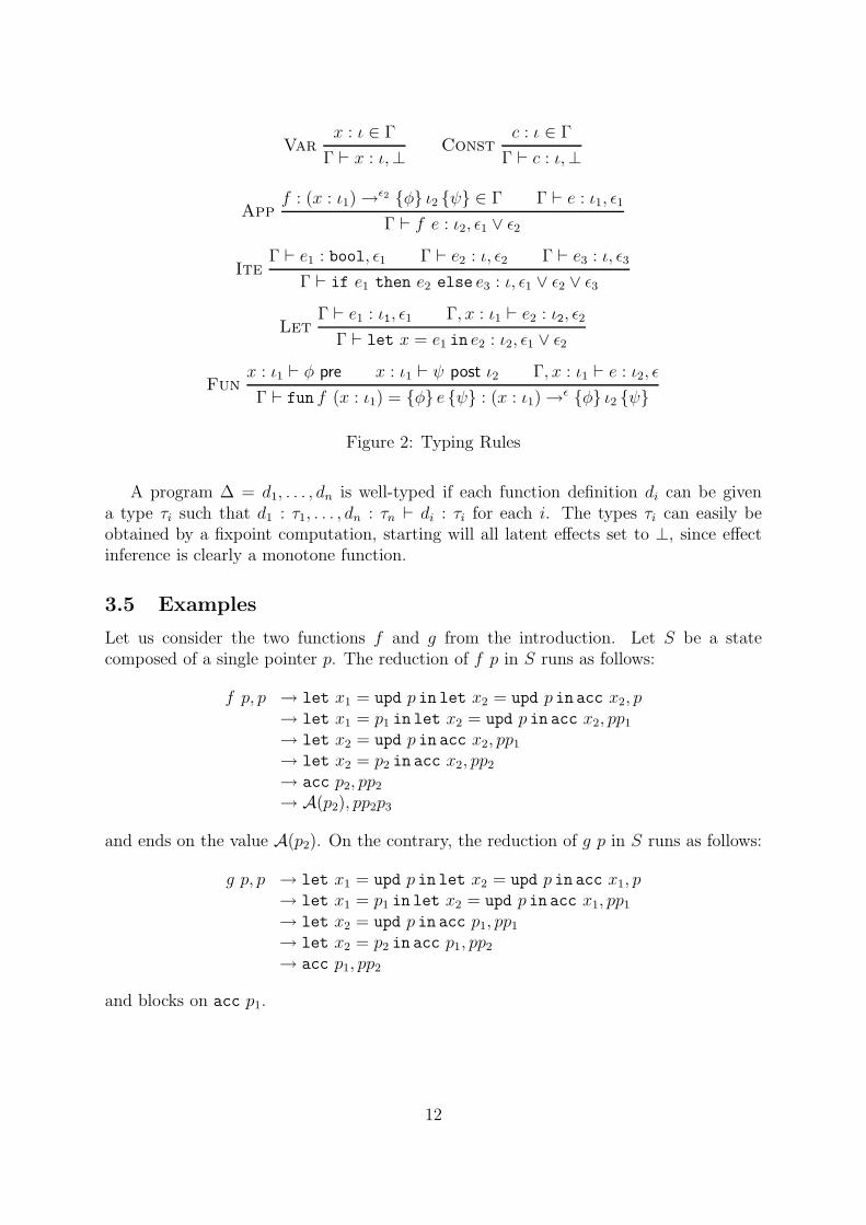
A program ∆ = d1, . . . , dn is well-typed if each function definition di can be givena type τi such that d1 : τ1, . . . , dn : τn ⊢ di : τi for each i. The types τi can easily beobtained by a fixpoint computation, starting will all latent effects set to ⊥, since effectinference is clearly a monotone function.

3.5 Examples

Let us consider the two functions f and g from the introduction. Let S be a statecomposed of a single pointer p. The reduction of f p in S runs as follows:

f p, p → let x1 = upd p in let x2 = upd p in acc x2, p

→ let x1 = p1 in let x2 = upd p in acc x2, pp1

→ let x2 = upd p in acc x2, pp1

→ let x2 = p2 in acc x2, pp2

→ acc p2, pp2

→ A(p2), pp2p3

and ends on the value A(p2). On the contrary, the reduction of g p in S runs as follows:

g p, p → let x1 = upd p in let x2 = upd p in acc x1, p

→ let x1 = p1 in let x2 = upd p in acc x1, pp1

→ let x2 = upd p in acc p1, pp1

→ let x2 = p2 in acc p1, pp2

→ acc p1, pp2

and blocks on acc p1.

12

4 Proof System

This section introduces a theory for semi-persistence and a proof system for this theory.First we define the syntax and semantics of logical annotations. Then we compute a setof constraints for each program expression, which is proved to express the correctness ofthe program with respect to semi-persistence. Finally we give a decision procedure tosolve the constraints.

4.1 Theory of Semi-Persistence

The syntax of annotations is as follows:

term t ::= x | p | prev(t)atom a ::= t = t | path(t, t)

postcondition ψ ::= a | ψ ∧ ψprecondition φ ::= a | φ ∧ φ | ψ ⇒ φ | ∀x. φ

Terms are built from variables, pointers and a single function symbol prev. Atoms arebuilt from equality and a single predicate symbol path. A postcondition ψ is restrictedto a conjunction of atoms. A precondition is a formula φ built from atoms, conjunctions,implications and universal quantifications. A negative formula (i.e. appearing on the leftside of an implication) is restricted to a conjunction of atoms. We introduce two differentsyntactic categories ψ and φ for formulae but one can notice that φ actually contains ψ.This syntactic restriction on formulae is justified later in Section 4.5 when introducingthe decision procedure. In the remainder of the paper, a “formula” refers to the syntacticcategory φ. Substitution a of term t for a variable x in a formula φ is written φ{x← t}.We denote by S(A) the set of all subterms of a set of atoms A.

The typing of terms and formulae is straightforward, assuming that prev has signaturesemi → semi. Function postconditions may refer to the function result, represented bythe variable ret . Formulae can only refer to variables of type semi (including variableret). We write Γ ⊢ φ to denote a well-formed formula φ in a typing environment Γ.

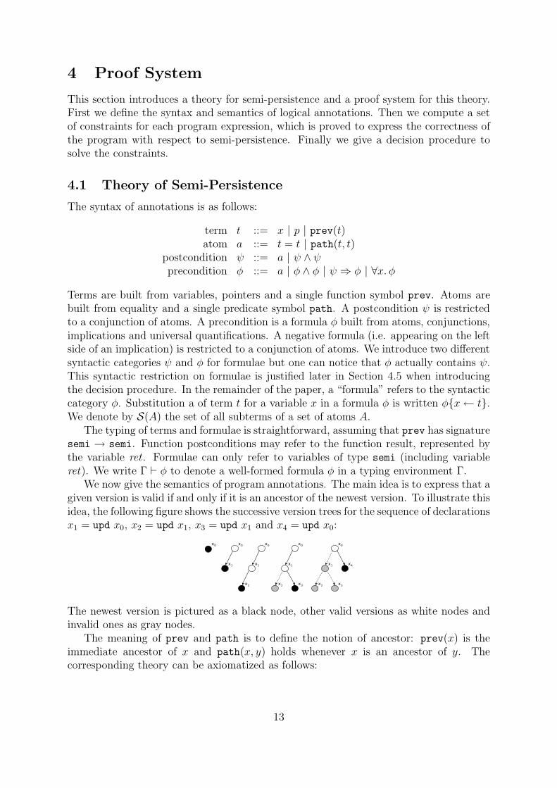
We now give the semantics of program annotations. The main idea is to express that agiven version is valid if and only if it is an ancestor of the newest version. To illustrate thisidea, the following figure shows the successive version trees for the sequence of declarationsx1 = upd x0, x2 = upd x1, x3 = upd x1 and x4 = upd x0:

The newest version is pictured as a black node, other valid versions as white nodes andinvalid ones as gray nodes.

The meaning of prev and path is to define the notion of ancestor: prev(x) is theimmediate ancestor of x and path(x, y) holds whenever x is an ancestor of y. Thecorresponding theory can be axiomatized as follows:

13

Definition 1 The theory T is defined as the combination of the theory of equality andthe following axioms:

(A1) ∀x. path(x, x)(A2) ∀xy. path(x, prev(y))⇒ path(x, y)(A3) ∀xyz. path(x, y) ∧ path(y, z)⇒ path(x, z)

We write |= φ if φ is valid in any model of T .

The three axioms (A1)–(A3) exactly define path as the reflexive transitive closure ofprev−1, since we consider validity in all models of T and therefore in those where path isthe smallest relation satisfying axioms (A1)–(A3). Note that prev is a total function andthat there is no notion of “root” in our logic. Thus a version always has an immediateancestor, which may or may not be valid.

To account for the modification of the newest version as program execution progresses,we introduce a “mutable” variable cur to represent the newest version. This variable doesnot appear in programs: its scope is limited to annotations. The only way to modify itscontents is to call the primitive operations backtrack and branch. We are now able togive the full type expressions for the three primitive operations:

backtrack :(x : semi)→⊤ {path(x, cur)} semi {ret = x ∧ cur = x}

branch :(x : semi)→⊤

{cur = x} semi {ret = cur ∧ prev(cur) = x}acc :

(x : semi)→⊥ {path(x, cur)} δ {true}

As expected, effect ⊤ for the first two reflects the modification of cur . The validityof function argument x is expressed as path(x, cur) in operations backtrack and acc.Note that acc has no postcondition (written true and which could stand for the tautologycur = cur) since we are not interested in the values contained in the data structure.

We are now able to define the judgements used in Section 3.4 for pre- and postcondi-tions. We write Γ ⊢ φ pre as syntactic sugar for Γ, cur : semi ⊢ φ. Similarly, Γ ⊢ ψ post ι

is syntactic sugar for Γ, cur : semi, ret : ι ⊢ ψ when return type ι is semi and forΓ, cur : semi ⊢ ψ otherwise. Note that since Γ only contains the function argumentx in typing rule Fun, the function precondition may only refer to x and cur , and itspostcondition to x, cur and ret .

In Section 4.5, we will need the following subterms property:

Lemma 2 If H is a set of atoms, t1 a subterm of H and H |= path(t1, t2) then t2 is asubterm of H.

4.2 Constraints

We now define the set of constraints associated to a given program. This is mostly aweakest precondition calculus, which is greatly simplified here since we have only onemutable variable (namely cur). For a program expression e and a formula φ we write

14

framef (φ) = φf{x← ret} ∧ ∀ret ′. ψf{ret ← ret ′, x← ret} ⇒ φ{ret ← ret ′}if f : (x : ι)→⊥ {φf} ι

′ {ψf}

framef (φ) = φf{x← ret} ∧ ∀ret ′cur ′. ψf{ret ← ret ′, x← ret , cur ← cur ′} ⇒φ{ret ← ret ′, cur ← cur ′}

if f : (x : ι)→⊤ {φf} ι′ {ψf}

C(v, φ) = φ{ret ← v}C(if e1 then e2 else e3, φ) = C(e1, C(e2, φ) ∧ C(e3, φ))

C(let x = e1 in e2, φ) = C(e1, C(e2, φ){x← ret})C(f e1, φ) = C(e1, framef (φ))

C(fun f (x : ι) = {φ} e {ψ}) = ∀x. ∀cur . φ⇒ C(e, ψ)

Figure 3: Constraint synthesis

this weakest precondition C(e, φ). This is formula expressing the conditions under whichφ will hold after the evaluation of e. Note that cur may appear in φ, denoting the resultof e, but does not appear in C(e, φ) anymore. For a function definition d we write C(d) theformula expressing its correctness, that is the fact that the function precondition impliesthe weakest precondition obtained from the function postcondition, for any functionargument and any initial value of cur . The definition for C(e, φ) is given in Figure 3.This is a standard weakest precondition calculus, except for the conditional rule. Indeed,one would expect a rule such as

C(if e1 then e2 else e3, φ) =C(e1, (ret = true⇒ C(e2, φ)) ∧ (ret = false⇒ C(e3, φ)))

but since φ cannot test the result of condition e1 (φ may only refer to variables of typesemi), the conjunction above simplifies to C(e2, φ) ∧ C(e3, φ).

The constraint synthesis for a function call, C(f e1, φ), is the only nontrivial case. Itrequires precondition φf to be valid and postcondition ψf to imply the expected propertyφ. Universal quantification is used to introduce f ’s results and side-effects. We use theeffect in f ’s type to distinguish two cases: either effect is ⊥ which means that cur is notmodified and thus we only quantify over f ’s result (hence we get for free the invarianceof cur); or effect is ⊤ and we quantify over an additional variable cur ′ which stands forthe new value of cur . To simplify this definition, we introduce a formula transformerframef (φ) which builds the appropriate postcondition for argument e1.

The formula established by an expression may be weakened, as stated by the followinglemma:

Lemma 3 If |= ∀ret . ∀cur . φ1 ⇒ φ2 and |= C(e, φ1) then |= C(e, φ2).

4.3 Examples

This section details the constraints obtained on several program examples.

15

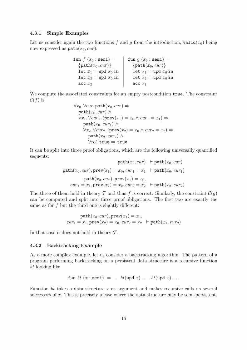
4.3.1 Simple Examples

Let us consider again the two functions f and g from the introduction, valid(x0) beingnow expressed as path(x0, cur):

fun f (x0 : semi) ={path(x0, cur)}let x1 = upd x0 in

let x2 = upd x0 in

acc x2

fun g (x0 : semi) ={path(x0, cur)}let x1 = upd x0 in

let x2 = upd x0 in

acc x1

We compute the associated constraints for an empty postcondition true. The constraintC(f) is

∀x0. ∀cur. path(x0, cur)⇒path(x0, cur) ∧∀x1. ∀cur 1. (prev(x1) = x0 ∧ cur 1 = x1)⇒path(x0, cur 1) ∧∀x2. ∀cur 2. (prev(x2) = x0 ∧ cur 2 = x2)⇒path(x2, cur 2) ∧∀ret . true⇒ true

It can be split into three proof obligations, which are the following universally quantifiedsequents:

path(x0, cur) ⊢ path(x0, cur)

path(x0, cur), prev(x1) = x0, cur 1 = x1 ⊢ path(x0, cur1)

path(x0, cur), prev(x1) = x0,

cur 1 = x1, prev(x2) = x0, cur 2 = x2 ⊢ path(x2, cur2)

The three of them hold in theory T and thus f is correct. Similarly, the constraint C(g)can be computed and split into three proof obligations. The first two are exactly thesame as for f but the third one is slightly different:

path(x0, cur), prev(x1) = x0,

cur 1 = x1, prev(x2) = x0, cur2 = x2 ⊢ path(x1, cur 2)

In that case it does not hold in theory T .

4.3.2 Backtracking Example

As a more complex example, let us consider a backtracking algorithm. The pattern of aprogram performing backtracking on a persistent data structure is a recursive functionbt looking like

fun bt (x : semi) = . . . bt(upd x) . . . bt(upd x) . . .

Function bt takes a data structure x as argument and makes recursive calls on severalsuccessors of x. This is precisely a case where the data structure may be semi-persistent,

16

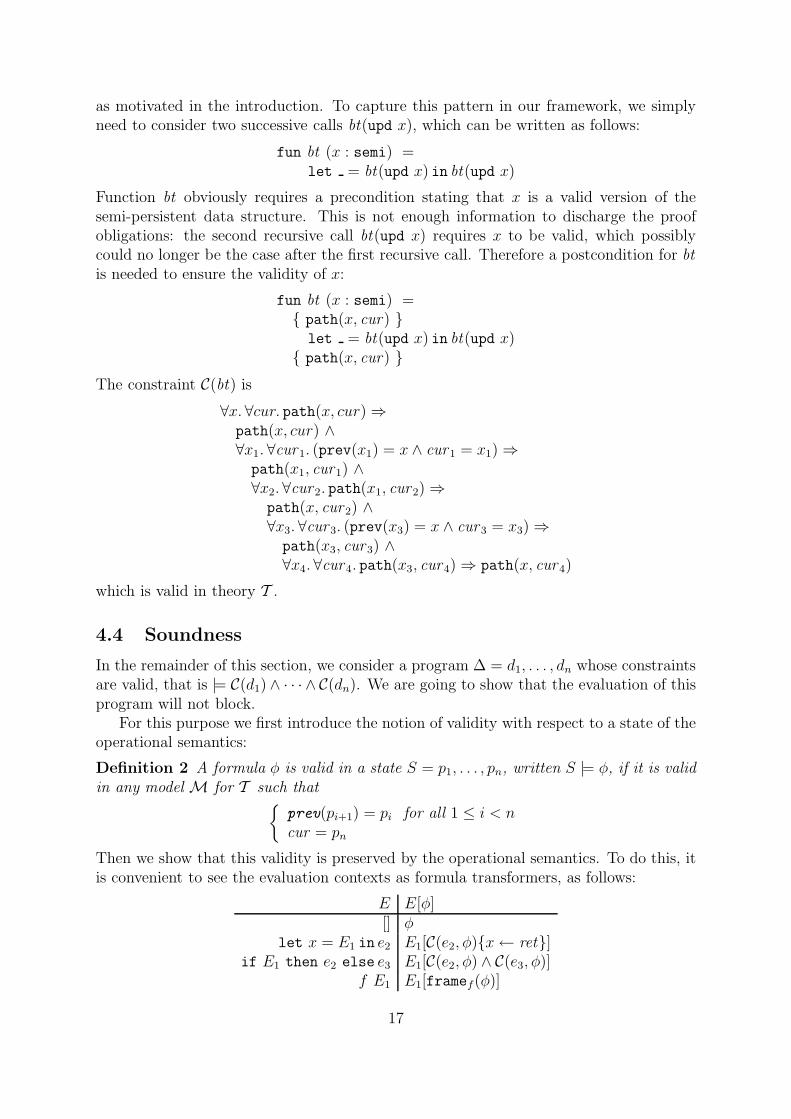
as motivated in the introduction. To capture this pattern in our framework, we simplyneed to consider two successive calls bt(upd x), which can be written as follows:

fun bt (x : semi) =let = bt(upd x) in bt(upd x)

Function bt obviously requires a precondition stating that x is a valid version of thesemi-persistent data structure. This is not enough information to discharge the proofobligations: the second recursive call bt(upd x) requires x to be valid, which possiblycould no longer be the case after the first recursive call. Therefore a postcondition for btis needed to ensure the validity of x:

fun bt (x : semi) ={ path(x, cur) }let = bt(upd x) in bt(upd x){ path(x, cur) }

The constraint C(bt) is

∀x. ∀cur. path(x, cur)⇒path(x, cur) ∧∀x1. ∀cur 1. (prev(x1) = x ∧ cur 1 = x1)⇒path(x1, cur1) ∧∀x2. ∀cur 2. path(x1, cur 2)⇒path(x, cur 2) ∧∀x3. ∀cur 3. (prev(x3) = x ∧ cur 3 = x3)⇒path(x3, cur 3) ∧∀x4. ∀cur 4. path(x3, cur 4)⇒ path(x, cur 4)

which is valid in theory T .

4.4 Soundness

In the remainder of this section, we consider a program ∆ = d1, . . . , dn whose constraintsare valid, that is |= C(d1) ∧ · · · ∧ C(dn). We are going to show that the evaluation of thisprogram will not block.

For this purpose we first introduce the notion of validity with respect to a state of theoperational semantics:

Definition 2 A formula φ is valid in a state S = p1, . . . , pn, written S |= φ, if it is validin any model M for T such that

{

prev(pi+1) = pi for all 1 ≤ i < n

cur = pn

Then we show that this validity is preserved by the operational semantics. To do this, itis convenient to see the evaluation contexts as formula transformers, as follows:

E E[φ][] φ

let x = E1 in e2 E1[C(e2, φ){x← ret}]if E1 then e2 else e3 E1[C(e2, φ) ∧ C(e3, φ)]

f E1 E1[framef(φ)]

17

There is a property of commutation between contexts for programs and contexts forformulae:

Lemma 4 S |= C(E[e], φ) if and only if S |= C(e, E[φ]).

Proof. Immediate by induction on E. �

We now want to prove preservation of validity, that is if S |= C(e, φ) and e, S → e′, S ′

then S ′ |= C(e′, φ). Obviously, this does not hold for any state S, program e and formulaφ. Indeed, if S ≡ p1p2, e ≡ upd p1 and φ ≡ prev(p2) = p1, then C(e, φ) is

path(p1, cur) ∧∀ret ′cur ′. (prev(ret ′) = p1 ∧ cur ′ = ret ′)⇒ prev(p2) = p1

which holds in S. But S ′ ≡ p1p for a fresh p, e′ ≡ p, and C(e′, φ) is prev(p2) = p1

which does not hold in S ′ (since p2 does not appear in S ′ anymore). Fortunately, weare not interested in the preservation of C(e, φ) for any formula φ, but only for formulaewhich arise from function postconditions. As pointed out in Section 4.1, a functionpostcondition may only refer to x, cur and ret only. Therefore we are only consideringformulae C(e, φ) where x is the only free variable (cur and ret do not appear in formulaeC(e, φ) anymore). This excludes the formula prev(p2) = p1 in the example above.

In the remainder of this section, we only consider program expressions and formulaewhich only refer to a single pointer p (representing the function argument). For technicalreasons, it is also convenient to restrict ourselves to states whose p is the first element.This is not a restriction, as stated by the following lemma:

Lemma 5 Let e be an expression and φ a formula which both refer to a single pointer p.Then, for any state S1pS2, S1pS2 |= C(e, φ) if and only if pS2 |= C(e, φ).

We are now able to prove preservation of validity:

Lemma 6 Let S be a state, φ be a formula and e a program expression. If S |= C(e, φ)and e, S → e′, S ′ then S ′ |= C(e′, φ).

Proof. The proof is done by induction on e:

• If e = if true then e1 else e2 then e′ = e1 and S ′ = S. We have C(e, φ) =C(true, C(e1, φ)∧C(e2, φ)) = C(e1, φ)∧C(e2, φ) since C(e1, φ)∧C(e2, φ) cannot referto a boolean result. Thus S ′ |= C(e′, φ). Similarly for if false.

• If e = let x = v in e1 then e′ = e1{x ← v} and S ′ = S. We have C(e, φ) =C(v, C(e1, φ){x ← ret}) = C(e1, φ){x ← v} = C(e1{x ← v}, φ), hence the resultholds.

• If e = f v and f is not a primitive then e′ = ef{x ← v} and S ′ = S. We haveC(e, φ) = C(v, framef(φ)) = framef (φ){ret ← v}. If f : (x : ι) →⊥ {φf} ι

′ {ψf}then this simplifies to φf{x ← v} ∧ ∀ret ′. ψf{x ← v, . . . } ⇒ φ{x ← v, . . .}. Sincef is correct, we have |= C(f) = ∀x. φf ⇒ C(ef , ψf). Thus S |= φf{x ← v} ⇒C(ef{x← v}, ψf{x← v}) and the result follows by Lemma 3. Similarly for f : (x :ι)→⊤ {φf} ι

′ {ψf}.

18

• If e = acc pn then S = S ′ = p1 · · · pnpn+1 · · · pm and e′ = A(pn). We have S |=C(acc pn, φ), that is S |= · · · ∧ ∀ret ′. true ⇒ φ{ret ← ret ′}. By instantiating ret ′

by A(pn) we have S |= φ{ret ← A(pn)} that is S |= C(A(pn), φ). Since S ′ = S theresult holds.

• If e = branch pn then S = p1 · · · pn, S ′ = Sp and e′ = p with p a fresh pointer.S |= C(branch pn, φ), that is S |= · · · ∧ ∀ret ′cur ′. (ret ′ = cur ′ ∧ prev(cur ′) = pn)⇒φ{ret ← ret ′, cur ← cur ′}. By instantiating both ret ′ and cur ′ by p, we haveS |= (p = p ∧ prev(p) = pn) ⇒ φ{ret ← p, cur ← p}. Since this formula does notcontain cur anymore, it is also valid in S ′ = Sp. Since prev(p) = pn in S ′ then theleft hand-side is valid and we have S ′ |= φ{ret ← p, cur ← p}. Since cur is p in S ′

we also have S ′ |= φ{ret ← p} which is C(p, φ).

• If e = backtrack pn then S = p1 · · · pnpn+1 · · ·pm, e′ = pn and S ′ = p1 · · · pn. Wehave S |= C(backtrack pn, φ), that is S |= · · ·∧∀ret ′cur ′. (ret ′ = pn∧ cur ′ = pn)⇒φ{ret ← ret ′, cur ← cur ′}. By instantiating both ret ′ and cur ′ by pn, we haveS |= φ{ret ← pn, cur ← pn}. Since this formula only refers to the first element ofS, which is also by Lemma 1 the first element of S ′, we have S ′ |= φ{ret ← pn, cur ←pn} and thus S ′ |= φ{ret ← pn} (since cur is pn in S ′), that is S ′ |= C(p, φ).

• If e = E[e1] and E[e1], S → E[e′1], S′ with e1, S → s′1, S

′, then S |= C(e1, E[φ]) byLemma 4. By induction hypothesis on e1 we have S ′ |= C(e′1, E[φ]). Then again byLemma 4 we have S ′ |= C(E[e′1], φ).

�

Finally, we prove the following progress property:

Theorem 1 Let S be a state, φ be a formula and e a program expression. If S |= C(e, φ)and e, S →∗ e′, S ′ 6→, then e′ is a value.

Proof. The proof is done by induction on the length of the evaluation →∗ and by caseanalysis on the last reduction:

• If e is irreducible then it is either a value v and the result holds, or it is an expressionE[f v] with f a primitive. By hypothesis, we have S |= C(E[f v], φ) and thusS |= C(f v, E[φ]) by Lemma 4. Since C(f v, E[φ]) = φf{x ← v} ∧ . . . , where φf

is f ’s precondition and x its formal argument. In each case, the validity of thisprecondition contradicts the irreducibility of e.

• If e, S → e1, S1 →∗ e′, S ′ 6→ then by Lemma 6 S1 |= C(e1, φ) and the result holds

by induction hypothesis on e1.

�

4.5 Decision Procedure

We now show that constraints are decidable and we give a decision procedure.First, we notice that any formula φ is equivalent to a conjunction of formulae of the

form∀x1. . . .∀xn. a1 ∧ · · · ∧ am ⇒ a

19

where the ai’s are atoms. This results from the syntactic restrictions on pre- and postcon-ditions, together with the weakest preconditions rules which are only using postconditionsin negative positions. Therefore we simply need to decide whether a given atom is theconsequence of other atoms.

We first recall the notion of congruence closure of a set H of hypotheses {a1, . . . , am}.

Definition 3 The congruence closure H⋆ of H is the smallest set of atoms such that

• if a ∈ H then a ∈ H⋆;

• if t ∈ S(H⋆) then t = t ∈ H⋆;

• if t1 = t2 ∈ H⋆ then t2 = t1 ∈ H

⋆;

• if t1 = t2 ∈ H⋆ and t2 = t3 ∈ H

⋆ then t1 = t3 ∈ H⋆;

• if t1 = t2 ∈ H⋆ and prev(t1), prev(t2) ∈ S(H⋆) then prev(t1) = prev(t2) ∈ H

⋆;

• if t1 = t2 ∈ H⋆, t3 = t4 ∈ H

⋆ and path(t1, t3) ∈ H⋆ then path(t2, t4) ∈ H

⋆.

Obviously S(H⋆) = S(H) since no new term is created. Thus H⋆ is finite and can becomputed as a fixpoint.

Algorithm 1 For any atom a such that S({a}) ⊆ S(H), the following algorithm, decide(H, a),decides whether H |= a.

1. First we compute the congruence closure H⋆.

2. If a is of the form t1 = t2, we return true if t1 = t2 ∈ H⋆ and false otherwise.

3. If a is of the form path(t1, t2), we build a directed graph G whose nodes are thesubterms of H⋆, as follows:

(a) for each pair of nodes t and prev(t) we add an edge from prev(t) to t;

(b) for each path(t1, t2) ∈ H⋆ we add an edge from t1 to t2;

(c) for each t1 = t2 ∈ H⋆ we add two edges between t1 and t2.

4. Finally we check whether there is a path from t1 to t2 in G.

Obviously this algorithm terminates since H⋆ is finite and thus so is G. We now showsoundness and completeness for this algorithm.

Theorem 2 decide(H, a) returns true if and only if H |= a.

Proof. (Soundness) Let M be a model of H and let us show that M is a model of a.Obviously,M is also a model of H⋆. If a is path(t1, t2) then the proof is by induction onthe length of the path. If the path has length 0, then t1 ≡ t2 and the result holds sinceM is a model of axiom (A1). Otherwise, we proceed by case analysis on the last step ofthe path since M is a model of the transitivity axiom (A3). If the last step is an edgefrom prev(t) to t then the result holds sinceM is a model of both (A1) and (A2). If thelast step is an edge corresponding to path(t3, t4) ∈ H

⋆ then the results holds since M is

20

a model of H⋆. If the last step is an edge corresponding to t3 = t4 ∈ H⋆, then M is a

model of path(t3, t4) by axiom (A1) and axioms of equality.(Completeness) Let us assume that H |= a. If a is t1 = t2 then t1 = t2 ∈ H⋆

by definition of the congruence closure, and thus the algorithm returns true. If a ispath(t1, t2) we proceed by induction on the proof of H |= a and by case analysis on thelast rule:

• (A1): There is an empty path from t1 to t2.

• (A2): We have H |= path(t1, prev(t2)). By Lemma 2, we have prev(t2) ∈ S(H)and thus we can apply the induction hypothesis. So there is a path from t1 toprev(t2) and thus a path from t1 to t2.

• (A3): We have H |= path(t1, t) and H |= path(t, t2). By Lemma 2, we havet ∈ S(H) and thus we can apply the induction hypothesis.

• Congruence: We have H |= u1 = t1, H |= u2 = t2 and H |= path(u1, u2). Thus wehave H |= path(u1, t1) and H |= path(u2, t2) (as above) and H |= path(u1, u2) byinduction hypothesis; the result follows.

�

Note: the restriction S({a}) ⊆ S(H) can be easily met by adding to H the equalitiest = t for any subterm t of a; it was only introduced to simplify the proof above.

4.6 Implementation

We have implemented the whole framework of semi-persistence. The implementationrelies on an existing proof obligations generator, Why [8]. This tool takes annotated first-order imperative programs as input and uses a traditional weakest precondition calculusto generate proof obligations. The language we use in this paper is actually a subsetof Why’s input language. We simply use the imperative aspect to make cur a mutablevariable. Then the resulting proof obligations are exactly the same as those obtained bythe constraint synthesis defined in Section 4.2.

The Why tool outputs proof obligations in the native syntax of various existingprovers. In particular, these formulas can be sent to Ergo [5], an automatic proverfor first-order logic which combines congruence closure with various built-in decision pro-cedures. We first simply axiomatized theory T using (A1)–(A3), which proved to bepowerful enough to verify all examples from this paper and several other benchmark pro-grams. Yet it is possibly incomplete (automatic theorem provers use heuristics to handlequantifiers in first-order logic). To achieve completeness, and to assess the results ofSection 4.5, we also implemented theory T as a new built-in decision procedure in Ergo.Again we verified all the benchmark programs.

5 Conclusion

We have introduced the notion of semi-persistent data structures, where update op-erations are restricted to ancestors of the most recent version. Semi-persistent data

21

structures may be more efficient than their fully persistent counterparts, and are of par-ticular interest in implementing backtracking algorithms. We have proposed an almostautomatic way of checking the legal use of semi-persistent data structures. It is basedon light user annotations in programs, from which proof obligations are extracted andautomatically discharged by a decision procedure.

There is a lot of remaining work to be done. First, the language introduced in Sec-tion 3, in which we check for legal use of semi-persistence, could be greatly enriched.Beside the missing features such as polymorphism or recursive datatypes, it would be ofparticular interest to consider the following extensions:

• simultaneous use of several semi-persistent data structures : One would probablyneed to express disjointness of version subtrees, and thus to enrich the logical frag-ment used in annotations with disjunctions and negations. We may lose decidabilityof the logic, though.

• dynamic creation of semi-persistent data structures: This would imply to express inthe logic the freshness of the allocated pointers and to maintain the newest versionsfor each data structures.

Note that these two features are already present in the data structures examples fromSection 2.

Another interesting direction would be to provide systematic techniques to make datastructures semi-persistent as previously done for persistence [7]. Clearly what we did forlists could be extended to tree-based data structures.

It would be even more interesting to formally verify semi-persistent data structureimplementations, that is to show that the contents of any ancestor of the version be-ing updated is preserved. Since such implementations are necessarily using imperativefeatures (otherwise they would be fully persistent), proving their correctness requiresverification techniques for imperative programs. This could be done for instance usingverification tools such as SPEC# [2] or Caduceus [9]. However, we would prefer verifyingOcaml code, as given in Section 2 for instance, but unfortunately there is currently notool to handle such code.

References

[1] Henry G. Baker. Shallow binding makes functional arrays fast. SIGPLAN Not.,26(8):145–147, 1991.

[2] Mike Barnett, K. Rustan M. Leino, and Wolfram Schulte. The Spec# programmingsystem: An overview. In CASSIS 2004, number 3362 in LNCS. Springer, 2004.

[3] Michael Benedikt, Thomas W. Reps, and Shmuel Sagiv. A decidable logic for de-scribing linked data structures. In European Symposium on Programming, pages2–19, 1999.

[4] Bruno Blanchet. Escape analysis: Correctness proof, implementation and experimen-tal results. In Symposium on Principles of Programming Languages, pages 25–37,1998.

22

[5] Sylvain Conchon and Evelyne Contejean. Ergo: A Decision Procedure for ProgramVerification. http://ergo.lri.fr/.

[6] Edsger W. Dijkstra. A discipline of programming. Series in Automatic Computation.Prentice Hall Int., 1976.

[7] J. R. Driscoll, N. Sarnak, D. D. Sleator, and R. E. Tarjan. Making Data StructuresPersistent. Journal of Computer and System Sciences, 38(1):86–124, 1989.

[8] J.-C. Filliatre. The Why verification tool. http://why.lri.fr/.

[9] J.-C. Filliatre and C. Marche. The Why/Krakatoa/Caduceus Platform for DeductiveProgram Verification (Tool presentation). In Proceedings of CAV’2007, 2007. Toappear.

[10] John Hannan. A type-based analysis for stack allocation in functional languages.In SAS ’95: Proceedings of the Second International Symposium on Static Analysis,pages 172–188, London, UK, 1995. Springer-Verlag.

[11] D. E. Knuth. Dancing links. In Bill Roscoe Jim Davies and Jim Woodcock, editors,Millennial Perspectives in Computer Science, pages 187–214. Palgrave, 2000.

[12] Xavier Leroy, Damien Doligez, Jacques Garrigue, Didier Remy, and Jerome Vouillon.The Objective Caml System, 2005. http://caml.inria.fr/.

[13] J. Gregory Morrisett, Karl Crary, Neal Glew, and David Walker. Stack-based typedassembly language. In Types in Compilation, pages 28–52, 1998.

[14] Greg Nelson. Verifying reachability invariants of linked structures. In POPL ’83:Proceedings of the 10th ACM SIGACT-SIGPLAN symposium on Principles of pro-gramming languages, pages 38–47, New York, NY, USA, 1983. ACM Press.

[15] Chris Okasaki. Purely Functional Data Structures. Cambridge University Press,1998.

[16] Silvio Ranise and Calogero Zarba. A theory of singly-linked lists and its extensibledecision procedure. In SEFM ’06: Proceedings of the Fourth IEEE InternationalConference on Software Engineering and Formal Methods, pages 206–215, Washing-ton, DC, USA, 2006. IEEE Computer Society.

[17] Frances Spalding and David Walker. Certifying compilation for a language withstack allocation. In LICS ’05: Proceedings of the 20th Annual IEEE Symposium onLogic in Computer Science (LICS’ 05), pages 407–416, Washington, DC, USA, 2005.IEEE Computer Society.

[18] Mads Tofte and Jean-Pierre Talpin. Implementation of the typed call-by-valuelambda-calculus using a stack of regions. In Symposium on Principles of Program-ming Languages, pages 188–201, 1994.

23