KNOTS, PERTURBATIVE SERIES AND QUANTUM MODULARITY
97
KNOTS, PERTURBATIVE SERIES AND QUANTUM MODULARITY STAVROS GAROUFALIDIS AND DON ZAGIER Abstract. We introduce an invariant of a hyperbolic knot which is a map α 7→ Φ α (h) from Q/Z to matrices with entries in Q[[h]] and with rows and columns indexed by the boundary parabolic SL 2 (C) representations of the fundamental group of the knot. These matrix invariants have a rich structure: (a) their (σ 0 ,σ 1 ) entry, where σ 0 is the trivial and σ 1 the geometric representation, is the power series expansion of the Kashaev invariant of the knot around the root of unity e 2πiα as an element of the Habiro ring, and the remaining entries belong to generalized Habiro rings of number fields; (b) the first column is given by the perturbative power series of Dimofte–Garoufalidis; (c) the columns of Φ are fundamental solutions of a linear q-difference equation; (d) the matrix defines an SL 2 (Z)-cocycle W γ in matrix-valued functions on Q that conjecturally extends to a smooth function on R and even to holomorphic functions on suitable complex cut planes, lifting the factorially divergent series Φ(h) to actual functions. The two invariants Φ and W γ are related by a refined quantum modularity conjecture which we illustrate in detail for the three simplest hyperbolic knots, the 4 1 ,5 2 and (-2, 3, 7) pretzel knots. This paper has two sequels, one giving a different realization of our invariant as a matrix of convergent q-series with integer coefficients and the other studying its Habiro-like arithmetic properties in more depth. Contents Part 0: Introduction and Overview 2 Part I: The main story 10 1. The original Quantum Modularity Conjecture 11 2. A collection of formal power series 13 2.1. The indexing set P K 13 2.2. Four constructions of the power series Φ (K,σ) α (h) 14 3. Interrelations among the power series Φ (σ) α (h) 17 3.1. The Generalized Quantum Modularity Conjecture 17 3.2. Lifting the QMC from constant terms to power series 19 3.3. Quadratic Relations 20 3.4. Asymptotics of the coefficients 22 4. Refining the Quantum Modularity Conjecture 25 4.1. Improving the Quantum Modularity Conjecture: optimal truncation 25 4.2. New elements of the Habiro ring 26 4.3. Smoothed optimal truncation 28 4.4. Strengthening the Generalized Quantum Modularity Conjecture 30 4.5. The Refined Quantum Modularity Conjecture 31 5. The matrix-valued cocycle associated to a knot 34 5.1. The Habiro-like matrix and the perturbative matrix 34 5.2. Smoothness 38 5.3. “Functions near Q” 41 5.4. Analyticity 45 1 arXiv:2111.06645v1 [math.GT] 12 Nov 2021
Transcript of KNOTS, PERTURBATIVE SERIES AND QUANTUM MODULARITY
KNOTS, PERTURBATIVE SERIES AND QUANTUM MODULARITY
STAVROS GAROUFALIDIS AND DON ZAGIER
Abstract. We introduce an invariant of a hyperbolic knot which is a map α 7→ Φα(h)from Q/Z to matrices with entries in Q[[h]] and with rows and columns indexed by theboundary parabolic SL2(C) representations of the fundamental group of the knot. Thesematrix invariants have a rich structure: (a) their (σ0, σ1) entry, where σ0 is the trivial andσ1 the geometric representation, is the power series expansion of the Kashaev invariant ofthe knot around the root of unity e2πiα as an element of the Habiro ring, and the remainingentries belong to generalized Habiro rings of number fields; (b) the first column is given bythe perturbative power series of Dimofte–Garoufalidis; (c) the columns of Φ are fundamentalsolutions of a linear q-difference equation; (d) the matrix defines an SL2(Z)-cocycle Wγ
in matrix-valued functions on Q that conjecturally extends to a smooth function on Rand even to holomorphic functions on suitable complex cut planes, lifting the factoriallydivergent series Φ(h) to actual functions. The two invariants Φ and Wγ are related by arefined quantum modularity conjecture which we illustrate in detail for the three simplesthyperbolic knots, the 41, 52 and (−2, 3, 7) pretzel knots. This paper has two sequels, onegiving a different realization of our invariant as a matrix of convergent q-series with integercoefficients and the other studying its Habiro-like arithmetic properties in more depth.
Contents
Part 0: Introduction and Overview 2
Part I: The main story 101. The original Quantum Modularity Conjecture 112. A collection of formal power series 13
2.1. The indexing set PK 13
2.2. Four constructions of the power series Φ(K,σ)α (h) 14
3. Interrelations among the power series Φ(σ)α (h) 17
3.1. The Generalized Quantum Modularity Conjecture 173.2. Lifting the QMC from constant terms to power series 193.3. Quadratic Relations 203.4. Asymptotics of the coefficients 22
4. Refining the Quantum Modularity Conjecture 254.1. Improving the Quantum Modularity Conjecture: optimal truncation 254.2. New elements of the Habiro ring 264.3. Smoothed optimal truncation 284.4. Strengthening the Generalized Quantum Modularity Conjecture 304.5. The Refined Quantum Modularity Conjecture 31
5. The matrix-valued cocycle associated to a knot 345.1. The Habiro-like matrix and the perturbative matrix 345.2. Smoothness 385.3. “Functions near Q” 415.4. Analyticity 45
1
arX
iv:2
111.
0664
5v1
[m
ath.
GT
] 1
2 N
ov 2
021
2 STAVROS GAROUFALIDIS AND DON ZAGIER
Part II. Complements 476. Half-symplectic matrices and their associated perturbative series 48
6.1. Half-symplectic matrices and the Bloch group 486.2. Ideal triangulations and the Neumann-Zagier equations 526.3. Nahm sums and the perturbative definition of the Φ-series 54
7. Two q-holonomic modules 577.1. Descendant Habiro-like functions 577.2. The J-matrix for the 52 knot 607.3. State-sums 617.4. The q-holonomic module of formal power series 64
8. Proof of the Modularity Conjecture for the 41 knot 658.1. The case of α = 0 658.2. The general case 67
9. Arithmetic aspects 709.1. Algebraic number theory aspects 709.2. Denominators and integrality properties 72
10. Numerical aspects 79
10.1. Computing the power series Φ(K,σ)α (h) 79
10.2. Optimal truncation and smoothed optimal truncation 82
Appendix: Numerical data for five sample knots 84The figure eight knot 84The sister of the figure eight knot 86The 52 knot 88The (−2, 3, 7) pretzel knot 91The 61 knot 93
References 94
Part 0: Introduction and Overview
In this paper and the companion paper [39], we will define and study three different typesof objects that can be associated to a hyperbolic knot:
• periodic functions on Q with values in Q with striking arithmetic properties and belongingto a generalization of the Habiro ring;
• divergent formal series in an infinitesimal variable h, or more precisely infinite collectionsof such power series, indexed by a rational number α (here “h” is meant to remind one ofPlanck’s constant and the perturbative expansions of quantum field theory); and
• q-series with integer coefficients, convergent in the unit disk and also thought of via q = e2πiτ
as holomorphic functions of a variable τ in the upper half-plane.
The first of these generalizes the Kashaev invariant of the knot, while the second and third
correspond roughly to the two partition functions Z(h) and Z(q) that are being studied inthe ongoing program of Gukov et al [46, 17] for general 3-manifolds. We will study thefirst two types of invariants in the present paper, and the functions of q or τ in [39]. In all
KNOTS, PERTURBATIVE SERIES AND QUANTUM MODULARITY 3
three cases we will actually define a whole matrix of functions of the type described above,and in all three cases one of the central questions will be the behavior of these functionsunder the action of the modular group on the rational numbers or on the upper half-plane.Another key aspect is that each of the three types of matrices constructed encodes the sameinformation as the other two and that all three can be interpreted as different realizations ofthe same abstract object, a square matrix of “functions-near-Q” that we believe is associatedto every hyperbolic knot, just as the different types of cohomology groups associated to aan algebraic variety over a number field, despite their very different properties, are seen asdifferent realizations of the same underlying “motive.”
The starting point for our entire investigation is the Kashaev invariant of a knot and the“quantum modularity” property for its Galois-equivariant extension that was conjecturedin [73]. We will review these topics in detail in Section 1, but remind the reader brieflyof the basic ingredients here. The Kashaev invariant of a hyperbolic knot K is an element〈K〉N of Z[e2πi/N ] for every N ∈ N whose absolute value is conjectured to grow exponentiallylike ecN , where c is 1/2π times the hyperbolic volume of the knot complement S3 r K.This invariant can be extended to a function J = J (K) (we will omit the knot from thenotation when it is fixed) from Q/Z to Q by Galois equivariance. (This means that we write〈K〉N as a polynomial in e2πi/N with rational coefficients and define J(a/N) for all a primeto N as the same polynomial evaluated at e−2πia/N .) The Quantum Modularity Conjecturegives a formula for the ratio of the values of J(X) and J(γX) as an asymptotic series in1/X as X tends to infinity through integers or through rational numbers with boundeddenominator, where γX = aX+b
cX+dwith γ =
(a bc d
)∈ SL2(Z). The quantitative version of
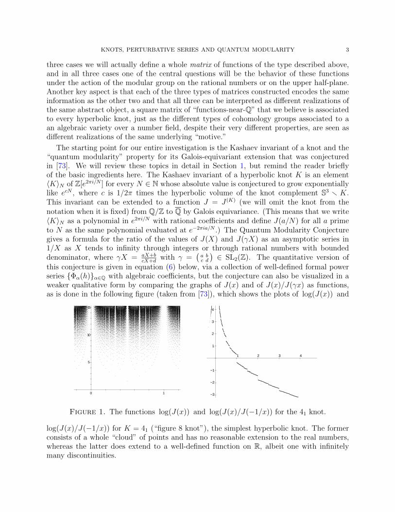
this conjecture is given in equation (6) below, via a collection of well-defined formal powerseries {Φα(h)}α∈Q with algebraic coefficients, but the conjecture can also be visualized in aweaker qualitative form by comparing the graphs of J(x) and of J(x)/J(γx) as functions,as is done in the following figure (taken from [73]), which shows the plots of log(J(x)) and
5
10
15
0 1 −3
−2
−1
1
2
3
4
1 2 3 4
Figure 1. The functions log(J(x)) and log(J(x)/J(−1/x)) for the 41 knot.
log(J(x)/J(−1/x)) for K = 41 (“figure 8 knot”), the simplest hyperbolic knot. The formerconsists of a whole “cloud” of points and has no reasonable extension to the real numbers,whereas the latter does extend to a well-defined function on R, albeit one with infinitelymany discontinuities.
4 STAVROS GAROUFALIDIS AND DON ZAGIER
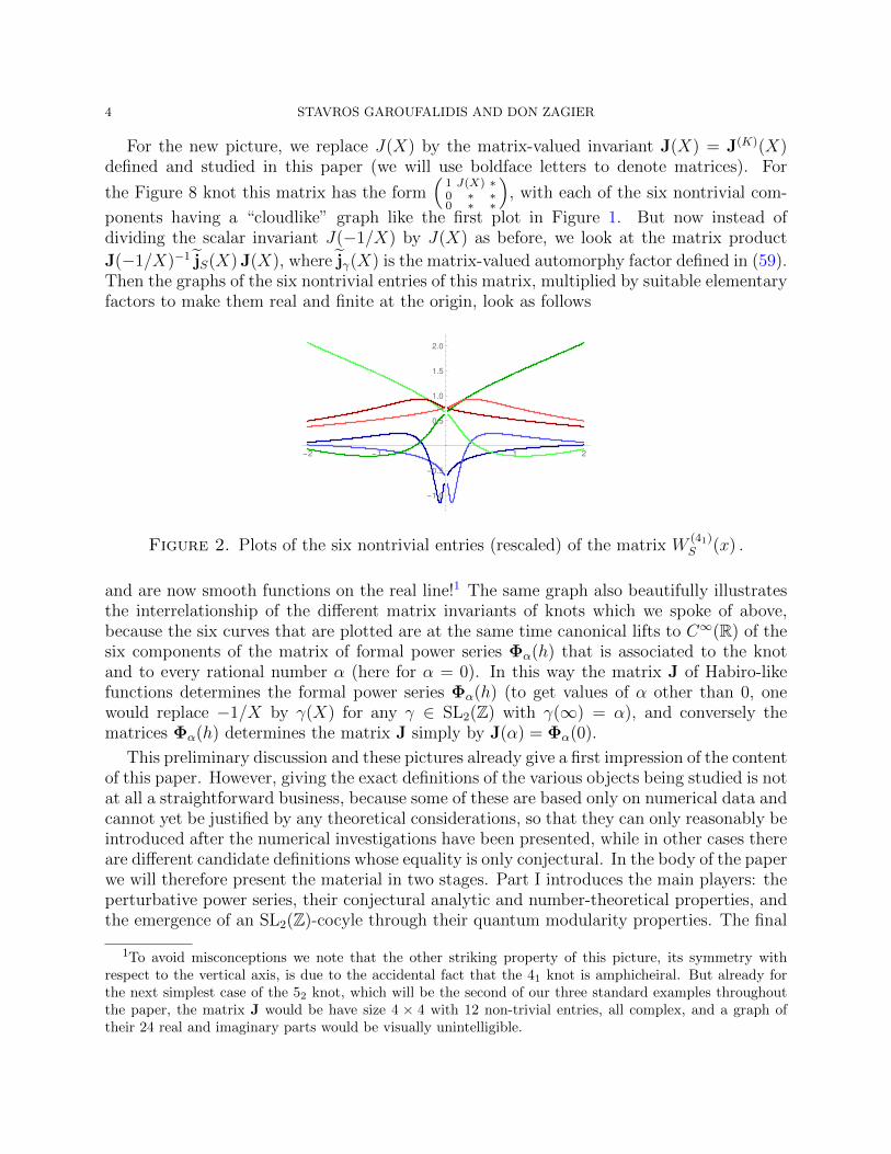
For the new picture, we replace J(X) by the matrix-valued invariant J(X) = J(K)(X)defined and studied in this paper (we will use boldface letters to denote matrices). For
the Figure 8 knot this matrix has the form(
1 J(X) ∗0 ∗ ∗0 ∗ ∗
), with each of the six nontrivial com-
ponents having a “cloudlike” graph like the first plot in Figure 1. But now instead ofdividing the scalar invariant J(−1/X) by J(X) as before, we look at the matrix product
J(−1/X)−1 jS(X) J(X), where jγ(X) is the matrix-valued automorphy factor defined in (59).Then the graphs of the six nontrivial entries of this matrix, multiplied by suitable elementaryfactors to make them real and finite at the origin, look as follows
-2 -1 1 2
-1.0
-0.5
0.5
1.0
1.5
2.0
Figure 2. Plots of the six nontrivial entries (rescaled) of the matrix W(41)S (x) .
and are now smooth functions on the real line!1 The same graph also beautifully illustratesthe interrelationship of the different matrix invariants of knots which we spoke of above,because the six curves that are plotted are at the same time canonical lifts to C∞(R) of thesix components of the matrix of formal power series Φα(h) that is associated to the knotand to every rational number α (here for α = 0). In this way the matrix J of Habiro-likefunctions determines the formal power series Φα(h) (to get values of α other than 0, onewould replace −1/X by γ(X) for any γ ∈ SL2(Z) with γ(∞) = α), and conversely thematrices Φα(h) determines the matrix J simply by J(α) = Φα(0).
This preliminary discussion and these pictures already give a first impression of the contentof this paper. However, giving the exact definitions of the various objects being studied is notat all a straightforward business, because some of these are based only on numerical data andcannot yet be justified by any theoretical considerations, so that they can only reasonably beintroduced after the numerical investigations have been presented, while in other cases thereare different candidate definitions whose equality is only conjectural. In the body of the paperwe will therefore present the material in two stages. Part I introduces the main players: theperturbative power series, their conjectural analytic and number-theoretical properties, andthe emergence of an SL2(Z)-cocyle through their quantum modularity properties. The final
1To avoid misconceptions we note that the other striking property of this picture, its symmetry withrespect to the vertical axis, is due to the accidental fact that the 41 knot is amphicheiral. But already forthe next simplest case of the 52 knot, which will be the second of our three standard examples throughoutthe paper, the matrix J would be have size 4 × 4 with 12 non-trivial entries, all complex, and a graph oftheir 24 real and imaginary parts would be visually unintelligible.
KNOTS, PERTURBATIVE SERIES AND QUANTUM MODULARITY 5
(conjectural) statements are given in Section 5, so that a reader who wants to see just theshort version of the story right away can skip directly to that section. Part II then containsmore detailed information about the definitions and properties of the objects appearing inPart I, including a discussion of the numerical methods used, some of which are quite subtle.The paper ends with an appendix containing tables of some of the functions studied for afew simple hyperbolic knots.
Since the paper contains so many different types of objects, with rather intricate inter-connections and taking shape only gradually in the course of the exposition, it seemed usefulto end this introduction by giving a detailed overview of the main ingredients. A further rea-son to include this rather long list here is that it contains a number of items (the unexpectedappearance of algebraic units, a description of the Bloch group and extended Bloch groupin terms of “half-symplectic matrices,” the notions of “asymptotic functions near Q” and of“holomorphic quantum modular forms,” a generalization of the Habiro ring to Habiro-likerings associated to number fields other than Q, or a procedure to “evaluate” divergent powerseries numerically) that are applicable or potentially applicable in domains quite separatefrom that of quantum knot invariants and that therefore may be of independent interest.
• Indexing set. Both the rows and the columns of the matrices associated to a knot Kare indexed by a finite set PK that can be described either in terms of boundary parabolicrepresentations of the fundamental group of the knot complement S3 rK or in terms of flatconnections, as explained in detail in Section 2,
• Level. As already mentioned, the matrices that we study also depend on a rationalnumber α. In all cases they are periodic in α, with the period N = NK however not alwaysbeing the same: it is 1 for the 41 and 52 knots, but 2 for the (−2, 3, 7)-pretzel knot. (Thesethree knots will serve as our standard illustrations throughout the paper.) Similarly, themodular invariance properties are not always under the full modular group SL2(Z), butsometimes under the subgroup Γ(N). We do not know what this “level” N is in general,although we have a guess (in terms of the quasi-periodicity of the degrees of the coloredJones polynomials), but its appearance in the numerical investigations was striking.
•Perturbatively and non-perturbatively defined power series. In the original versionof the Quantum Modularity Conjecture, the main statement was the existence of a collectionof formal power series Φα(h) describing the relationship between J(X) and J(γX) for large Xand fixed γ ∈ SL2(Z), with no prediction of what this power series was. However, in twopapers [13, 14] by Tudor Dimofte and the first author explicit candidates for these powerseries as perturbative series in h defined by Gaussian integration of a function explicitlygiven in terms of a triangulation of M3, rendering the original conjecture much more precise.These series will now form all but the top entry of the second column of our matrix. (Thefirst column being simply (1 0 . . . 0)t.) The top entry of the second column is defined in acompletely different, non-perturbative way in terms of the expansion near q = e2πiα of theKashaev invariant of K seen as an element of the Habiro ring. All of this will be explained indetail in Section 2, while the definitions of the other entries of the matrix Φa(h), which areagain given by perturbatively defined power series in all but the top row and (conjecturally)by elements of the Habiro ring for their top entries, will emerge via the Refined QuantumModularity Conjecture discussed in Sections 4.
6 STAVROS GAROUFALIDIS AND DON ZAGIER
• Arithmetic aspects. One of the main themes of this paper is that the topology of aknot involves a large amount of surprisingly complicated algebraic number theory. This isvalid both for the values of the Kashaev invariant itself and of its generalizations as givenby the matrxi J(x) at rational arguments x and more generally for the coefficients of the
entries Φ(σ,σ′)α (h) (α ∈ Q, σ, σ′ ∈ PK), which conjecturally belong to Q(h). Among the
most striking things that we found were the occurrence of certain algebraic units, whichled to the paper [9] with Frank Calegari associating units (modulo nth powers) in the nthcyclotomic extension of an arbitrary number field to elements in the Bloch group of thisfield, congruence properties of Ohtsuki type (which will be touched on only briefly here butwill become a main theme in the planned paper with Peter Scholze on the construction ofHabiro rings associated to any number field), and universal bounds, independent of the knot,for the denominators of the coefficients of the perturbative power series occurring.
• Half-symplectic matrices and the extended Bloch group. The power series con-structed in [13] and [14] are given in terms of the so-called Neumann-Zagier data describingthe combinatorics of a triangulation of a knot complement. This data takes the form of anN × 2N integral matrix, where N is the number of simplices of the triangulation, togetherwith a solution (corresponding to the “shape parameters,” i.e., the cross-ratios of the verticesof the ideal tetrahedra) of a collection of algebraic equations defined by this matrix. The keyproperty here is that the defining matrix is the upper half of a 2N × 2N symplectic matrixover Z. This leads to a somewhat different description than the standard one of the Blochgroup and extended Bloch group. All of this is discussed in Section 6, together with thedefinition of the perturbative series and a different appearance of the same construction inthe context of Nahm sums.
• Unimodularity and inverse matrix. Experimentally we find that the matrices thatwe construct are always unimodular, and also that there are explicit formulas for theirinverses as linear (or, for the top row, quadratic) rather than higher-degree polynomials in theentries of the matrices themselves. Combined with the behavior under complex conjugation,this leads to a kind of generalized unitarity property for our matrices (of course, againonly conjecturally, but we will not keep repeating this since most of the properties we arediscussing are only conjectural, though based on such extensive data that they are veryunlikely not to hold). All of this will be discussed in Section 5. The formula for the inversesof our matrices (apart from the top row) can be interpreted as giving quadratic relationsfor our power series, a special case of which appears in a recent paper of Gang, Kim andYoon [20] and which will be described in Subsection 3.3. These quadratic relations will takeon a life of their own in the companion paper [39] in terms of expressions for the “stateintegrals” defined by Kashaev and others as bilinear expressions in power series in q = e2πiτ
and q = e−2πi/τ .
• Extension property. As already stated, the rows and columns of our matrices are indexedby the set PK of flat connections. This set has a canonical element, the trivial connection,which we put at the beginning of the list, and the first row and column of each of our matricesthen has a completely different nature from the other entries. In particular, as we alreadysaw, the first column always consists of a 1 followed by 0s, so that the entire matrix is in(1 + r)× (1 + r) block triangular form, where 1 + r = |PK |. This means that these matrices
KNOTS, PERTURBATIVE SERIES AND QUANTUM MODULARITY 7
are describing structures which are r-dimensional extensions of 1-dimensional substructures.This can be seen clearly in the q-holonomy discussed below, where the recursions satisfiedby elements giving the top row contain a constant term 1 and those of the other rows arethe corresponding homogeneous recursions.
• q-holonomy. As already explained, the second column (the first column being trivial) ofour matrices of formal power series has a direct definition in terms of the triangulation ofthe knot complement and the corresponding Neumann-Zagier data. The other columns aredefined in a more complicated way that we still have not understood completely. Roughlyspeaking, each of the entries of the original column belongs to a “q-holonomic system,”meaning that it is part of a sequence of functions of q = e2πiα that satisfy linear recursionsover Q[q] and hence span a finite-dimensional space, and the other columns belong to, andin fact span, the same space. This applies not only to the matrices of formal power seriesin h, but also to the Habiro-like matrices J and to the matrices of q-series studied in [39],and will be discussed in detail in Section 7. The mysterious point here is that the columns ofour matrices, which are completely and uniquely defined by the various properties embodiedin the Refined Modularity Conjecture, give a canonical basis for these q-holonomic modules,but that even in those situations where we know what the module is or should be, we do nothave an a priori description of this basis.
• Refined quantum modularity. As stated at the beginning of this introduction, ourwhole story arises from the Quantum Modularity Conjecture (QMC) made in [73]. In itsoriginal form, the QMC says that for all γ =
(a bc d
)in SL2(Z) we have
J(γX) ≈ (cX + d)3/2 J(X) Φa/c
( 2πi
c(cX + d)
)(X →∞)
as X tends to infinity with a bounded denominator, where Φα(h) for α ∈ Q is a “completed”version of Φα(h) obtained by multiplying it by a suitable pure exponential in 1/h, and where“≈” denotes asymptotic equality to all orders in 1/X (or h). This statement already refinesthe Volume Conjecture of Kashaev [52] and its arithmetic properties and extension to allorders as described in [15]. In the Refined Quantum Modularity Conjecture (RQMC), whichwill be developed step by step in the course of Sections 3 and 4, it is extended in twodifferent ways. First of all, the above asymptotic statement will be generalized by replacingthe function J : Q→ Q by the other entries, initially of the first column and then by a kindof “bootstrapping” process (see below) of the whole matrix. More importantly, however, theright-hand side will be sharpened by the addition of lower-order terms which are completed
versions of other entries of the matrix Φα(X). Since the addition of an exponentially smallerexpression to a divergent power series does not make sense a priori, this requires a processof numerical evaluation by “optimal truncation” and then “smoothed optimal truncation”as listed in the bullet “Numerical aspects” below and discussed in detail in Sections 4.1and 10.2. The final result gives an asymptotic development to much higher precision of eachof the generalized Habiro-functions J(σ,σ′) evaluated at γX with X tending to infinity as a
linear combination of (r+1) of the power series Φα(h), with α = a/c and h = 2πi/c(cX+d).
8 STAVROS GAROUFALIDIS AND DON ZAGIER
This can then be written compactly in matrix form as
J(K)(γX) ≈ jγ(X) J(K)(X) Φ(K)a/c
( 2πi
c(cX + d)
)(= equation (57)), which is the final version of the RMC. Here the “automorphy factor”
jγ(X) is a diagonal matrix whose first entry is (cX + d)3/2 and whose other entries are pure
exponentials in X + d/c. Note that this property relates the matrices J and Φ, and allowsin particular to compute the second one from the first one.
• A matrix-valued cocycle. The matrix-valued form of RQMC as just stated leads im-mediately to the definition of an SL2(Z)-cocycle with coefficients in the space of matrix-valued functions on Q (or more precisely—and necessary in order to have an SL2(Z)-modulestructure—of almost-everywhere-defined functions on P1(Q)), defined by
Wγ(x) = J(γx)−1 jγ(x) J(x) ,
where this time the “automorphy factor” jg(x) is a slightly different diagonal matrix, againwith elementary entries, as defined explicitly in equations (59) and (24). The cocycle prop-erties of this automorphy factor imply that Wγ is a multiplicative cocycle, meaning thatWγγ′(X) is equal to Wγ(γ
′X) times Wγ′(X). Its remarkable properties are summarized inthe next two bullets.
• Analyticity and holomorphic quantum modular forms. The most important singlediscovery of this paper is that the cocycle Wγ(X), originally defined on rational numbersby the formula just given, extends to a smooth function on the real numbers. This fact,which might have been found purely experimentally by looking at the graphs of the com-ponents of Wγ(X), as illustrated by Figure 2 above, and which can also be checked purelyexperimentally, as explained in Section 5.4, was actually predicted in advance on the basis ofthe occurrence of the same cocycle γ 7→ Wγ with a completely different construction in thecompanion paper [39] to this one. Specifically, in that paper we construct a matrix Qhol(τ)of holomorphic functions of a complex variable τ ∈ C r R, whose entries are power serieswith integer coefficients in q = e2πiτ , and such that the coboundary Qhol(γτ)−1Qhol(τ) ex-tends holomorphically across both the half-lines (γ−1(∞),∞) and (−∞, γ−1(∞)), with therestrictions to these two half-lines coinciding with the function Wγ there. This extendabilityof Qhol(γτ)−1Qhol(τ) across subintervals of the real line means that Qhol is an example ofa “holomorphic quantum modular form,” a new type of object that turns out to occur inmany other contexts and that will be described briefly in Subsection 5.4 and in detail in thepapers [71] and [39].
• “Functions near Q.” Each component Φσ,σ′α (h) of the matrix Φα has a natural completion,
as explained in Section 2, defined as its product with a certain exponential in 1/h and (in thecase of the top row) a half-integral power of h, and it is these completions that appear in theoriginal Quantum Modularity Conjecture and its various extensions. It turns out that the“right way” to think of these collections of series is that they represent one single “asymptotic
function near Q” defined by Q(σ,σ′)(α − ~) = Φσ,σ′α (2πi~), where α varies over Q and ~ is
infinitesimal. This notion of asymptotic functions near Q (or simply “functions near Q” forshort), which will be defined and explained more carefully in Subsection 5.3, sheds light on
KNOTS, PERTURBATIVE SERIES AND QUANTUM MODULARITY 9
several properties of our knot invariants (and also turns out to occur also in other contexts).In particular, the cocycle Wγ, which was initially defined (almost everywhere) on Q by the
formula Wγ(x) = J(γx)−1jγ(X)J(x), is not a coboundary in the space of functions on Q, butis one in the larger space of functions near Q: Wγ(x) = Q(γx)−1 Q(x). The occurrence ofthe same cocycle with two different representations as a coboundary in appropriate matrix-valued SL2(Z)-modules provides the link between the two papers and the reason for outbelief that both the matrix Q of generalized Habiro functions and the matrix Qhol of q-seriesare realizations of the same underlying motive-like object.
• Numerical aspects. Everything in the paper is based on numerical computations, andthese have several non-obvious aspects, as discussed in Section 10. In particular, we explainthere how Kashaev invariants can be computed rapidly and how one can then use extrap-
olation techniques to evaluate many coefficients of the power series Φ(σ,σ′)a (h) numerically
and recognize them as real numbers. The calculations also have a “bootstrapping” aspect inwhich the successively discovered relations among the series as described by the final RefinedQuantum Modularity Conjecture permit one to evaluate these series to increasing levels ofprecision in a recursive way. Finally, in order to identify the correct series in the RQMC, itis crucial to be able to evaluate the divergent series in h occurring, not only up to order hN
for any fixed ingeger N , but up to exponentially small error terms, where the constant oc-curring in the exponential can also be successively improved in several steps. This is done bya process of “smoothed optimal truncation” which was originally a second appendix to thispaper, but has now been relegated to a separate publication [40] and is also briefly describedin Section 10.2.
We end with a few miscellaneous remarks on different aspects of the above constructions.
• Resurgence aspects. An important aspect of our paper are the matrices Φα(h) offactorially divergent series and their distinguished liftWγ(x) to a matrix of analytic functions.In this connection we find several properties that can be classified under the general headingof “resurgence.” On the one hand, we find experimentally that the coefficients of eachentry of Φα(h) are given asymptotically as integer linear combinations of certain divergentexpansions involving the coefficients themselves multiplied by gamma factors. The integralityof the so-called Stokes constants is a phenomenon observed in the current paper and furtherstudied in [26, 25]. A different connection of our results with the usual resurgence propertiesof the perturbative series Φα(h) is the method of smoothed optimal truncation mentionedjust above, which can be seen as an alternative approach to lifting these power series toactual functions than the standard method via Borel resummation and Pade approximation.Of course, the final emergence of a canonical lift coming from the analyticity properties ofthe cocycle Wγ(x) eventually makes both numerical procedures obsolete in our case, but thiscocycle could not be found without having them first.
• Equivalence of the various invariants. We observe that all of our invariants, assumingtheir conjectured properties, determine each other and in particular all are determined bythe colored Jones polynomials and perhaps even by the Kashaev invariant alone. The pointof the paper is therefore not that our new invariants can distinguish knots, but that they
10 STAVROS GAROUFALIDIS AND DON ZAGIER
reveal new properties and make connection with SL2(C)-representations of the fundamentalgroup, hyperbolic geometry and non-trivial number theory.
• Eighth roots of unity and the Dedekind eta function. A further minor surprise wasthe appearance of Dedekind sums at several places in the calculations, which we had notexpected. Notably, this occurred in the construction of state sums for the non-Habiro-likeelements of our matrix J (see Section 7.2) and in the ubiquitous but mysterious 8th root ofunity that enters all of our asymptotic formulas and that is related to the 8th root of unityoccurring in the modular transformation behavior of η3.
• 3 + 1 : a possible alternative interpretation. Finally, we mention a point that willnot be discussed in the paper at all, but may give a different way of looking at the theobjects studied here. Namely, the (σ, σ′) entry of the matrix J(X) that we have associated
Figure 3. The Witten cylinder
to a knot K, and hence also to its complement M = S3 rK, can be thought of as numbersassociated to the “Witten cylinder,” Equwhich is the 4-manifold M × R equipped with apair of boundary-parabolic SL2(C) connections σ and σ′ on its two ends, together with aninteger k, called the “level” in complex Chern-Simons theory [70, 69] and related to therational number X by k+ 2 = den(X). This suggests a possible interpretation of the entriesof J(X) as expectation values of some yet-to-be-defined (3+1)-dimensional theory on M×R.
We end this introduction with a disclaimer. In this paper we are trying only to presentinteresting new phenomena and are not striving for maximum generality. Not only are werestricting our attention to knot complements rather than arbitrary 3-manifolds, but we willusually assume that the knots being considered have whatever properties (e.g., that theirparabolic character varieties are 0-dimensional) are convenient for our exposition. In anycase most of the material presented is empirical, based on extensive experiments with afew very simple knots having all of these special properties, and we prefer not to speculateon what modifications might be needed in more general situations. Of course, we expectthat the whole story is quite general, and ongoing calculations by Campbell Wheeler indeedalready confirm that very similar types of statements will hold, for instance, for the Witten-Reshitikhin-Turaev invariant of certain closed hyperbolic 3-manifolds.
KNOTS, PERTURBATIVE SERIES AND QUANTUM MODULARITY 11
Part I: The main story
1. The original Quantum Modularity Conjecture
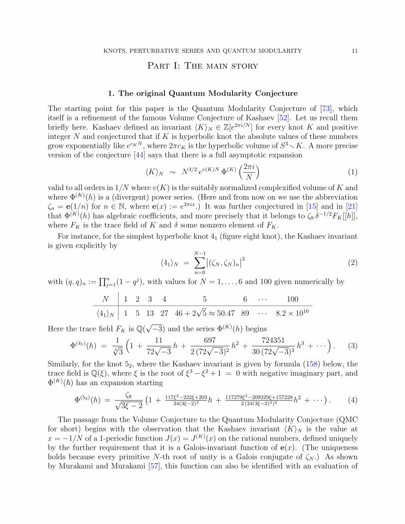
The starting point for this paper is the Quantum Modularity Conjecture of [73], whichitself is a refinement of the famous Volume Conjecture of Kashaev [52]. Let us recall thembriefly here. Kashaev defined an invariant 〈K〉N ∈ Z[e2πi/N ] for every knot K and positiveinteger N and conjectured that if K is hyperbolic knot the absolute values of these numbersgrow exponentially like ecKN , where 2πcK is the hyperbolic volume of S3rK. A more preciseversion of the conjecture [44] says that there is a full asymptotic expansion
〈K〉N ∼ N3/2 ev(K)N Φ(K)(2πi
N
)(1)
valid to all orders in 1/N where v(K) is the suitably normalized complexified volume ofK andwhere Φ(K)(h) is a (divergent) power series. (Here and from now on we use the abbreviationζn = e(1/n) for n ∈ N, where e(x) := e2πix.) It was further conjectured in [15] and in [21]that Φ(K)(h) has algebraic coefficients, and more precisely that it belongs to ζ8 δ
−1/2FK [[h]],where FK is the trace field of K and δ some nonzero element of FK .
For instance, for the simplest hyperbolic knot 41 (figure eight knot), the Kashaev invariantis given explicitly by
〈41〉N =N−1∑n=0
∣∣(ζN , ζN)n∣∣2 (2)
with (q, q)n :=∏n
j=1(1− qj), with values for N = 1, . . . , 6 and 100 given numerically by
N 1 2 3 4 5 6 · · · 100
〈41〉N 1 5 13 27 46 + 2√
5 ≈ 50.47 89 · · · 8.2× 10¹⁶
Here the trace field FK is Q(√−3) and the series Φ(K)(h) begins
Φ(41)(h) =14√
3
(1 +
11
72√−3
h +697
2 (72√−3)2
h2 +724351
30 (72√−3)3
h3 + · · ·). (3)
Similarly, for the knot 52, where the Kashaev invariant is given by formula (158) below, thetrace field is Q(ξ), where ξ is the root of ξ3− ξ2 + 1 = 0 with negative imaginary part, andΦ(K)(~) has an expansion starting
Φ(52)(h) =ζ8√
3ξ − 2
(1 + 117ξ2−222ξ+203
24(3ξ−2)3h + 117279ξ2−209229ξ+157228
2 (24(3ξ−2)3)2h2 + · · ·
). (4)
The passage from the Volume Conjecture to the Quantum Modularity Conjecture (QMCfor short) begins with the observation that the Kashaev invariant 〈K〉N is the value atx = −1/N of a 1-periodic function J(x) = J (K)(x) on the rational numbers, defined uniquelyby the further requirement that it is a Galois-invariant function of e(x). (The uniquenessholds because every primitive N -th root of unity is a Galois conjugate of ζN .) As shownby Murakami and Murakami [57], this function can also be identified with an evaluation of
12 STAVROS GAROUFALIDIS AND DON ZAGIER
the colored Jones polynomial J(K)N (q) [51, 65] by J(x) = JK,N(e(−x)) for any N ∈ Z with
Nx ∈ Z. In [73] it was found that (1) is just the special case(a bc d
)=(
0 −11 0
)of the more
general (and of course still conjectural) statement that
J (K)(aN + b
cN + d
)∼ (cN + d)3/2 ev(K)(N+d/c) Φ
(K)a/c
( 2πi
c(cN + d)
)(5)
to all orders in N as N → ∞ for any matrix(a bc d
)∈ SL2(Z) with c > 0, where Φ
(K)α (~) is
a power series with algebraic coefficients depending on α ∈ Q/Z, with Φ(K)0 = Φ(K). This
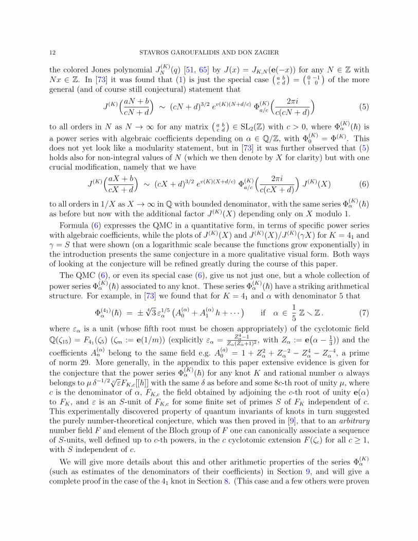
does not yet look like a modularity statement, but in [73] it was further observed that (5)holds also for non-integral values of N (which we then denote by X for clarity) but with onecrucial modification, namely that we have
J (K)(aX + b
cX + d
)∼ (cX + d)3/2 ev(K)(X+d/c) Φ
(K)a/c
( 2πi
c(cX + d)
)J (K)(X) (6)
to all orders in 1/X as X →∞ in Q with bounded denominator, with the same series Φ(K)α (~)
as before but now with the additional factor J (K)(X) depending only on X modulo 1.
Formula (6) expresses the QMC in a quantitative form, in terms of specific power serieswith algebraic coefficients, while the plots of J (K)(X) and J (K)(X)/J (K)(γX) for K = 41 andγ = S that were shown (on a logarithmic scale because the functions grow exponentially) inthe introduction presents the same conjecture in a more qualitative visual form. Both waysof looking at the conjecture will be refined greatly during the course of this paper.
The QMC (6), or even its special case (6), give us not just one, but a whole collection of
power series Φ(K)α (~) associated to any knot. These series Φ
(K)α (~) have a striking arithmetical
structure. For example, in [73] we found that for K = 41 and α with denominator 5 that
Φ(41)α (~) = ± 4
√3 ε1/5
α
(A
(α)0 + A
(α)1 h+ · · ·
)if α ∈ 1
5Z r Z . (7)
where εα is a unit (whose fifth root must be chosen appropriately) of the cyclotomic field
Q(ζ15) = F41(ζ5) (ζm := e(1/m)) (explicitly εα = Z4α−1
Zα(Zα+1)2, with Zα := e
(α − 1
3)) and the
coefficients A(α)n belong to the same field e.g. A
(a)0 = 1 + Z2
α + Z−2α − Z4
α − Z−4α , a prime
of norm 29. More generally, in the appendix to this paper extensive evidence is given for
the conjecture that the power series Φ(K)α (~) for any knot K and rational number α always
belongs to µ δ−1/2 c√εFK,c[[h]] with the same δ as before and some 8c-th root of unity µ, where
c is the denominator of α, FK,c the field obtained by adjoining the c-th root of unity e(α)to FK , and ε is an S-unit of FK,c for some finite set of primes S of FK independent of c.This experimentally discovered property of quantum invariants of knots in turn suggestedthe purely number-theoretical conjecture, which was then proved in [9], that to an arbitrarynumber field F and element of the Bloch group of F one can canonically associate a sequenceof S-units, well defined up to c-th powers, in the c cyclotomic extension F (ζc) for all c ≥ 1,with S independent of c.
We will give more details about this and other arithmetic properties of the series Φ(K)α
(such as estimates of the denominators of their coefficients) in Section 9, and will give acomplete proof in the case of the 41 knot in Section 8. (This case and a few others were proven
KNOTS, PERTURBATIVE SERIES AND QUANTUM MODULARITY 13
independently by Bettin and Drappeau [5].) We will also give detailed numerical evidencefor several other knots, for several values of α ∈ Q/Z, and to a relatively high degree in the
power series Φ(K)α (~), in the appendix to this paper. The calculations required to obtain these
values are not at all trivial, since one has to be able to calculate the Kashaev invariants for(many) arguments with large denominators and then use very precise extrapolation methodsto be able to find the coefficients to high enough accuracy to recognize them numerically asalgebraic numbers.
Presenting the numerical evidence for the QMC was the initial motivation for this paper,and this already led to interesting numerical observations, such as the appearance of thenear unit ε or the denominator estimates mentioned above. But in the course of doing thesecalculations we discovered that the QMC is only part of a much larger story involving a
whole collection of power series {Φ(K,σ)α (~)}α∈Q/Z, σ∈PK indexed by a certain finite set PK
(defined below) as well as by an index in Q/Z as before. In the rest of Part I we explainwhat these power series are, how they are related to each other, and how they lead to newinvariants and to a whole series of successive refinements of the original quantum modularityconjecture.
2. A collection of formal power series
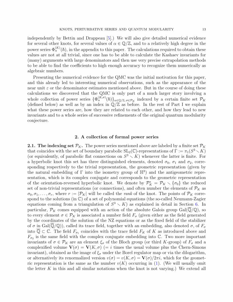
2.1. The indexing set PK. The power series mentioned above are labeled by a finite set PKthat coincides with the set of boundary parabolic SL2(C)-representations of Γ := π1(S3rK)(or equivalently, of parabolic flat connections on S3 rK) whenever the latter is finite. Fora hyperbolic knot this set has three distinguished elements, denoted σ0, σ1 and σ2, corre-sponding respectively to the trivial representation, the geometric representation (given bythe natural embedding of Γ into the isometry group of H3) and the antigeometric repre-sentation, which is its complex conjugate and corresponds to the geometric representationof the orientation-reversed hyperbolic knot. We denote by P∗K = PK r {σ0} the reducedset of non-trivial representations (or connections), and often number the elements of PK asσ0, σ1, . . . , σr, where r := |PK | will be called the rank of the knot. The points of PK corre-spond to the solutions (in C) of a set of polynomial equations (the so-called Neumann-Zagierequations coming from a triangulation of S3 r K) as explained in detail in Section 6. Inparticular, PK comes equipped with an action of the absolute Galois group Gal(Q/Q), soto every element σ ∈ PK is associated a number field Fσ (given either as the field generatedby the coordinates of the solution of the NZ equations or as the fixed field of the stabilizerof σ in Gal(Q/Q)), called its trace field, together with an embedding, also denoted σ, of Fσinto Q ⊂ C. The field Fσ1 coincides with the trace field FK of K as introduced above andFσ2 is the same field with the complex conjugate embedding into C. Two more importantinvariants of σ ∈ PK are an element ξσ of the Bloch group (or third K-group) of Fσ and acomplexified volume V(σ) = V(K, σ) (= i times the usual volume plus the Chern-Simonsinvariant), obtained as the image of ξσ under the Borel regulator map or via the dilogarithm,or alternatively its renormalized version v(σ) = v(K, σ) = V(σ)/2πi, which for the geomet-ric representation is the same as the number v(K) occurring in (1). (We will usually omitthe letter K in this and all similar notations when the knot is not varying.) We extend all
14 STAVROS GAROUFALIDIS AND DON ZAGIER
of these invariants to PK by setting Fσ0 = Q, V(s0) = 0, ξσ0 = 0. In Section 6 of Part II wewill give more details about the set PK and its invariants, and also say something about thesituation when the variety of parabolic representations contains positive-dimensional compo-nents. In Sections 5 and 6 we will also describe a large (matrix- rather than vector-valued)collection of power series associated to K.
Before explaining how to associate a formal power series to each σ ∈ PK and α ∈ Q/Z,we first would like to make the above definitions more tangible by describing PK explicitlyfor three simple examples, the knots 41 and 52 already used above and the (−2, 3, 7) pretzelknot (henceforth simply (−2, 3, 7)), which will be our basic examples throughout the paper.They have ranks 2, 3, and 6, respectively. For K = 41 the only elements of PK are the threeuniversal ones σ0, σ1 and σ2, the first with trace field Q and the other two both with tracefield Q(
√−3), but with the complex embedding
√−3 7→ −i
√3 in the second case. The
corresponding volumes are V(σ0) = 0, V(σ1) = iV , and V(σ2) = −iV , where V = 2.02 · · ·is the usual volume, and are all real because the knot 41 is amphicheiral. (In general the
mirror knot K of a knot has trace fields FK,σ = FK,σ and V(K, σ) = V (K, σ).) For K = 52
we again have only two essentially different fields Q and Q(ξ) with ξ3− ξ2 + 1 = 0 (the cubicfield with discriminant −23), the latter with three embeddings σ1, σ2, and σ3 correspondingto choosing the root ξ ∈ C with negative, positive, or zero imaginary part, respectively. Butfor the third knot K = (−2, 3, 7), PK consists of seven elements, the trivial representation σ0,the three representations σ1, σ2, σ3 corresponding to the trace field of K (which is the sameas that of 52, with its embeddings numbered the same way), and three further elements σ4,σ5 and σ6 corresponding to the field Q(η) with η3 + η2 − 2η − 1 = 0 (the abelian cubicfield with discriminant 49) together with the three embeddings into C given by sendingη to 2 cos(2π/7), 2 cos(4π/7) and 2 cos(6π/7), respectively. In general, to each knot Kwe associate the algebra AK = Q × A∗K defined as the product of the abstract fields Fσwith σ ranging over representatives of the Galois orbits of PK , so that PK (resp. P∗K) canbe identified with the set of all algebra maps from AK (resp. A∗K) to C; then for our threebasic examples we have
Ared41
= Q(√−3) , Ared
52= Q(ξ) , Ared
(−2,3,7) = Q(ξ)×Q(η) . (8)
2.2. Four constructions of the power series Φ(K,σ)α (h). We will now describe several
different approaches to obtaining the formal power series Φ(K,σ)α (h) associated to an element σ
of PK and a number α ∈ Q/Z.
If σ = σ1 is the geometric representation, then Φ(K,σ)α (h) is by definition just the power
series ΦKα (h) whose existence is asserted by the Quantum Modularity Conjecture, and for σ
in the Galois orbit of σ1 we simply apply Galois conjugation to this series (at the level of itsn-th power if α has denominator n), with some special consideration for the roots of unity
occurring. For example, for the knot K = 41 the series Φ(K,σ)α (h) for α = 0 and α = a/5
are the ones given by (3) and (7), respectively, for σ = σ1. We then get Φ(K,σ2)0 simply by
replacing√−3 by −
√−3 (or, in this case, replacing h by −h and multiplying by i) in (3),
and Φ(41,σ2)a/5 is obtained from (7) by performing the same operation on both εa/5 and the
coefficients A(a/5)n . Similarly, if K is the 52 knot then the value of Φ
(K,σ)α (h) at α = 0 is given
KNOTS, PERTURBATIVE SERIES AND QUANTUM MODULARITY 15
by (4) if σ = σ1, and the values for σ = σ2 or σ3 are obtained simply by replacing ξ by itsGalois conjugates. In general the coefficients of these power series lie in the product of acertain root of unity, the c-th root (where c is the denominator of α) of a unit in Fσ, and aconjugate of the same factor δ−1/2 as in the original QMC as described in Section 1. Moredetails about the arithmetic of these numbers will be given in Section 9.
The reader may have noticed that the QMC asserts the existence of the power series
Φ(K,σ)α (h) for σ = σ1 but gives no clue about how to define them (and especially how to define
those for σ not a Galois conjugate of σ1) given a hyperbolic knot K. A definition of the
power series Φ(K,σ)α (h) for all σ 6= σ0 was given by Tudor Dimofte and the first author in the
two papers [13] (for α = 0) and [14] (for general α). What is more, the definition of the seriesuses as input the gluing equation matrices of an ideal triangulation of the knot complement,along with a solution to the Neumann-Zagier equations. Roughly speaking, one associatesto an ideal triangulation of the knot complement a collection of polynomial equations (theNeumann-Zagier equations) whose solutions correspond to the elements of Pred
K , the solutionfor each σ ∈ Pred
K being a collection of algebraic numbers (the shape parameters) belonging tothe field Fσ. One then associates to each solution of these equations and for each α ∈ Q/Za certain integral that is evaluated perturbatively by the standard method of Gaussianintegration and Feynman diagrams (with a possible ambiguity of multiplication by a powerof e(α)). This process, whose details will be reviewed in Section 6, is completely effectiveand gives, for instance, the three power series
Φ((−2,3,7),σj)0 (h) =
ξj√6ξj − 4
(1 − 33ξ2j−123ξj+128
24(3ξj−2)3h− 104172ξ2j−183417ξj+130189
2 (24(3ξj−2)3)2h2 + · · ·
)(9)
for the elements σ1, σ2, and σ3 of P(−2,3,7), where ξ1, ξ2, ξ3 are the Galois conjugates of ξ asnumbered above, and the three totally different power series
Φ((−2,3,7),σj+3)0 (h) =
√ηj − 2
14
(1 −
43η2j − 21
168h−
3928η2j + 63ηj − 1491
2 · 1682h2 + · · ·
)(10)
for the elements σ4, σ5, and σ6, where ηj = 2 cos(2πj/7) are the Galois conjugates of η inthe ordering given above. The coefficients of the power series Φ(K,σ)(h) for all σ ∈ PK havesimilar arithmetic properties to the special case when σ is Galois conjugate to σ1.
As well as the “straight” power series Φ(K,σ)α (h), we will also need the completed functions
Φ(K,σ)α (h) = eV(σ)/c2h Φ(K,σ)
α (h)(c = den(α), σ 6= σ0
), (11)
which for the moment we think of as a purely formal expression (the exponential of a Laurentseries in h with a simple pole) but which will be given a more precise sense later (cf. Sec-tion 10.2). It is this combination that appear in all of our asymptotic formulas, e.g. the
right-hand side of (5) would become (cN + d)−3/2 Φ(K)a/c
(2πicN+d
)in this notation. We should
also mention here that in [14] the series Φ(K,σ)α (h) is defined only up to an 2n-th root of unity,
where n is the denominator of α. The generalized QMC that we will present in the nextsection eliminates this ambiguity (at least up to a net sign depending on σ but not on α).
An idea that will be crucial for this paper is that we have to associate power series
Φ(σ)α (h) ∈ Q[[h]] to the trivial representation σ = σ0 as well as to the non-trivial ones to
16 STAVROS GAROUFALIDIS AND DON ZAGIER
get a coherent total picture. Here there is no Neumann-Zagier data and we use instead acompletely different construction based on the Habiro ring. Recall that this ring is defined by
H := lim←− Z[q]/((q; q)n) , (12)
where (x; q)n =∏n−1
i=0 (1−qix) denotes the q-Pochhammer symbol or “shifted quantum facto-rial”. As mentioned in the introduction, Habiro showed in [47] that the Galois-equivariantlyextended Kashaev invariant J (K)(α) (α ∈ Q) is the evaluation at q = e(α) of a uniquelydefined element, which we will denote by J (K)(q), of this ring. We then define the power
seres Φ(K,σ)α (h) for σ = σ0 by
Φ(K,σ0)α (h) = J (K)
(e(α) e−h
)∈ Q[e(α)][[h]] (13)
For example, for K = 41 we have the explicit representation (equivalent to (2) for q = ζN)
J (41)(q) =∞∑n=0
(q−1; q−1)n (q; q)n =∞∑n=0
(−1)n q−n(n+1)/2 (q; q)2n (14)
of J (K)(q) as an element of the Habiro ring, and setting q = e−h ∈ Q[[h]] we find
Φ(41,σ0)0 (h) = 1 − h2 +
47
12h4 − 12361
360h6 +
10771487
20160h8 − · · · (15)
(which happens to be even because the knot 41 is amphicheiral), while the Kashaev invariantfor our second standard example 52 is given by formula (158) below and we find
Φ(52,σ0)0 (h) = 1 + h +
5
2h2 +
49
6h3 +
797
24h4 +
19921
120h5 + · · · . (16)
For the (−2, 3, 7) knot we have no convenient Habiro-like formula for the Kashaev invariant,but there is still a method (explained in Part II) to obtain its expansion to any order in hat any root of unity just from the values at roots of unity, the expansion at q = 1 beginning
Φ((−2,3,7),σ0)0 (h) = 1 − 12h + 129h2 − 7275
4h3 − 384983
8h4 + · · · . (17)
Note that the complexified volume vanishes for the trivial representation, so that (11) would
suggest that we should define the completion Φ(K,σ0)α (h) to be Φ
(K,σ0)α (h). But in fact, for
reasons that will appear clearly in Section 3, it turns out to be better to define Φ(K,σ0)α (h) in
this case by
Φ(K,σ0)α (h) =
( ch2πi
)3/2
Φ(K,σ0)α (h) . (18)
We have now described constructions of the power series Φ(K,σ)α (h) for every σ ∈ PK , but
based on very disparate ideas: if σ is the geometric representation or is Galois conjugateto it, we use the Quantum Modularity Conjecture and Galois covariance, for other repre-sentations σ different from the trivial one we use a perturbative approach (which is givenin [13] and [14] and conjectured there to agree with the first definition when σ = σ1), and
for the trivial representation we define Φ(K,σ)α (h) by a completely different formula based on
the Habiro ring. In fact, as already mentioned in the introduction, there is even a fourth
approach in which the series Φ(K,σ)α are obtained from the asymptotics as q tends radially
KNOTS, PERTURBATIVE SERIES AND QUANTUM MODULARITY 17
to e(α) of certain q-series with integral coefficients. (This connection will not be discussedfurther here but will be the main theme of [39].) It is then natural to ask why we considerthese different series as being similar at all and why we denote them in the same way. Inthe next two sections we will present a whole series of properties that justify this.
3. Interrelations among the power series Φ(σ)α (h)
In this section we describe four empirically found properties, of very different natures, thatlink and motivate the formal power series introduced above.
3.1. The Generalized Quantum Modularity Conjecture. The function J (K) from Q/Zto Q, which was originally defined as the Galois-equivariant extension of the Kashaev in-
variant 〈K〉N , has now re-appeared as the constant term Φ(K,σ0)α (0) of one of a collection of
formal power series Φ(K,σ)α (h) ∈ Q[[h]] indexed by the elements σ of a finite set PK associated
to the knot. This suggests that we should look also at the constant terms of the other seriesas well, i.e., that we should study the functions (generalized Kashaev invariants)
J (K,σ) : Q/Z → Q, J (K,σ)(α) := Φ(K,σ)α (0) (19)
for all σ ∈ PK . These functions turn out to have beautiful arithmetic properties generalizingin a non-obvious way the Habiro-ring property of the original functions J (K) = J (K,σ0).These will be the subject of the subsequent paper [35] and, apart from a few numericalexamples, will not be discussed further here. Instead, we will concentrate on the asymptoticproperties of the new functions (19). In particular, we can ask whether these functionssatisfy an analogue of the Quantum Modularity Conjecture for J (K). The answer turns outto be positive, but to involve a number of successive refinements arising from the numericaldata. We will present the simplest version here and the strongest versions, which requiresome preparation, in Sections 4 and 5.
We start once again with the simplest knot K = 41. Here the function J (K,σ0)(α) =J (K)(α) is the one given by (2) (with ζN replaced by e(α)) whereas the new functionsJ (K,σ1)(α) and J (K,σ2)(α) are given explicitly by
J (K,σ1)(α) =1
√c 4√
3
∑Zc = ζ6
c∏j=1
∣∣1 − qjZ∣∣2j/c (c = den(α), q = e(α)) (20)
and J (K,σ2)(α) = i J (K,σ1)(−α) = J (K,σ1)(α). The original QMC says that J (41)(aX+bcX+d
)is
asymptotically equal to (cX + d)3/2 Φ(41)a/c
(2πi
c(cX+d)
)J (41)(X) for any matrix
(a bc d
)∈ SL2(Z) as
X tends to infinity with bounded denominator, where the “completion” Φ is defined by (11).When we look at the corresponding asymptotics for the two new functions and for the twosimple matrices
(0 −11 0
)and
(1 02 1
)of SL2(Z), we see a similar behavior, but with two major
differences: the “automorphy factor” (cX + d)3/2 is no longer there, and there is a newexponential factor involving the complex volume. Explicitly, what we find experimentally is
J (41,σ1)(−1/X) ∼ ev(K)/(num(X)·den(X)) J (41,σ1)(X) Φ(41)0
(2πi
X
)(21)
18 STAVROS GAROUFALIDIS AND DON ZAGIER
(here “num” and “den” denote the numerator and denominator) and
J (41,σ1)(X/(2X + 1)) ∼ ev(K)/((X+ 12
)·den(X)2) J (41,σ1)(X) Φ(41)1/2
( 2πi
2(2X + 1)
)(22)
and similarly for Φ(σ2) but with v(K) replaced by v(K, σ2) = −v(K). The two equations (21)and (22) can be written uniformly in the form
J (41,σ1)(γX) ∼ ev(K)λγ(X) J (41,σ1)(X) Φ(41)a/c
( 2πi
c(cX + d)
)(23)
for γ =(a bc d
)∈ SL2(Z), where λγ(x) is defined for x = r/s ∈ Q with r and s coprime by
λγ(x) :=1
den(x)2(x− γ−1(∞))=
c
s(cr + ds)= ± c
den(x)den(γx). (24)
The experiments show that the same thing happens for other knots K and all represen-tations σ, i.e., we can formulate the Generalized Quantum Modularity Conjecture (GQMC)
(cX + d)−κ(σ) e−v(σ)λγ(X) J (K,σ)(γX) ∼ J (K,σ)(X) Φ(K)a/c
( 2πi
c(cX + d)
), (25)
as X →∞ with bounded denominator (as usual), and where γ =(a bc d
)∈ SL2(Z) with c > 0,
and where the weight κ(σ) of the representation σ ∈ PK is defined by
κ(σ) =
{3/2 if σ = σ0,
0 otherwise.(26)
Notice that (25) coincides with the original QMC when σ = σ0 because in this case the factore−v(σ)λγ(X) on the left-hand side of (25) is identically 1. We also see that the two different
definitions (11) and (18) of Φ(K,σ) for σ 6= σ0 and σ = σ0 can now be written in a uniformway as
Φ(K,σ)α (h) = |c~|κ(σ) ev(σ)/c2~ Φ(K,σ)
α (h) (c = den(α), ~ := h/2πi), (27)
which will also be convenient at many other points. Notice that the convention ~ = h/2πi isalmost, but not quite, the same as the one used in ordinary quantum mechanics, and also thatthe factor 2πi relating h and ~ is the same as that used in our two different normalizationsV(σ) and v(σ) = V(σ)/2πi of the volume, so that ev(σ)/c2~ = eV(σ)/c2h.
We end this subsection by proving a cocycle property of the arithmetic function λγ(X)that will be needed in Section 5.
Lemma 3.1. For all γ, γ′ ∈ PSL2(Z) and x ∈ Qr {γ′−1(∞), (γγ′)−1(∞)} we have:
λγγ′(x) = λγ(γ′x) + λγ′(x) . (28)
Proof. Let γ =(a bc d
), γ′ =
(a′ b′
c′ d′
)and γγ′ =
(a′′ b′′
c′′ d′′
). Then c′′d′ − c′d′′ = c, and hence
λγγ′(x)− λγ′(x) =c′′
s(c′′r + d′′s)+
c′
s(c′r + d′s)=
c
s(c′r + d′s)(c′′r + d′′s)= λγ(γ
′x)
as required. A more enlightening way to say this is that λγ(γ′(∞)) = C(γγ′, γ′) where
C(γ1, γ2) :=c(γ1γ
−12 )
c(γ1)c(γ2)= γ−1
2 (∞)− γ−11 (∞), which is a coboundary and hence a cocycle. �
KNOTS, PERTURBATIVE SERIES AND QUANTUM MODULARITY 19
3.2. Lifting the QMC from constant terms to power series. In the previous sub-section we generalized the original QMC by replacing the Kashaev invariant J (K) by thegeneralized Kashaev invariants J (K,σ) for any σ ∈ PK . This in turn will be further refinedin Section 4 by adding terms of exponentially lower order to the right-hand side of theasymptotic formula. Here we discuss instead a different refinement.
Our starting point, just as in subsection 3.1, is that the Kashaev invariant J (K)(α) is
equal to the constant term Φ(σ0)α (0) of the power series Φ
(σ0)α (h) as defined in Section 2, so
that the original QMC (6) can be rewritten as
Φ(σ0)γX (0) ∼ (cX + d)3/2 Φ
(σ0)X (0) Φa/c
( 2πi
c(cX + d)
)for X tending to infinity with fixed fractional part or with bounded denominator. (Here weagain omit the knot K from the superscripts when it is not varying to avoid cluttering upthe notations. Recall also that c > 0.) It is then natural to ask whether this asymptotic
formula can be lifted to a corresponding statement for the full series Φ(σ0)α (h) rather than
just its constant term. The answer is affirmative, but with a little twist:
Φ(σ0)γX (h∗) ∼ (cX + d)3/2 Φ
(σ0)X (h) Φa/c
( 2πi
c(cx+ d)
), (29)
where x = X − ~ with ~ as in (27) and h∗ = h(cx+d)(cX+d)
.
Let us explain what the asymptotic expansion (29) means in the simplest case of the
figure 8 knot. Recall that Φ(σ0)X (h) = J (e(X)e−h) where J (q) = J (41)(q) is the element of
the Habiro ring given by (14), related to J(X) = J (41)(X) by J(X) = J (e(X)). Since theHabiro ring is closed under the operator q d/dq, it contains the function J ′ defined by
J ′(q) := qd
dqJ (q) =
∞∑n=1
(q−1; q−1)n (q, q)n
n∑k=1
k1 + qk
1− qk. (30)
We then define the formal derivative J ′ : Q/Z→ 2πiQ by J ′(X) = 2πiJ ′(e(X)). Then thestatement of (29) in this case is
1
(cX + d)2
J ′(aX+bcX+d
)J(aX+bcX+d
) − J ′(X)
J(X)≈ − 2πi
(cX + d)2
Φ′a/c(
2πic(cX+d)
)Φa/c
(2πi
c(cX+d)
) , (31)
interpreted in the following sense. The left-hand side of (31) is 2πi times an algebraic numberbelonging to some fixed cyclotomic field for each fixed element γ =
(a bc d
)∈ SL2(Z) and bound
on the denominator of X, while the right-hand side is defined only as a divergent power seriesin (cX + d)−1. The claim is then that when we compute both sides of (31) for fixed γ andfor X tending to infinity with bounded denominator, using (30) to compute the terms J ′(X)and J ′(γX) as exact algebraic numbers, the the two expressions agree numerically to allorders in 1/X, and this is the statement that we verified numerically for several elemets γand sequences of large rational numbers X. Note that (31) is almost what we would get ifwe differentiated the original QMC formula (6) logarithmically (which of course we are notallowed to do since it is only an asymptotic statement valid for large rational numbers Xwith fixed denominator and hence is rigid), except that then we would have an extra term
20 STAVROS GAROUFALIDIS AND DON ZAGIER
32
ccX+d
which is in fact not present because Equation (29) contains (cX + d)3/2 rather than
(cx+ d)3/2.
All of this was for the trivial connection σ0. If we consider instead an arbitrary element σof PK , then what we find is the obvious combination of (25) (which was only for the constantterms Φ(0)) and (29) (which gave the “twist” needed to include h), namely
(cX + d)−κ(σ) e−v(σ)λγ(X) Φ(σ)γX(h∗) ∼ Φ
(σ)X (h) Φa/c
( 2πi
c(cx+ d)
), (32)
with x = X − ~ and h∗ = h/(cx+ d)(cX + d) as in (29).
Equation (32) differs in two notable ways from the original QMC (6): the appearanceof the “tweaking factor” e−v(σ)λγ(X) and the change of infinitesimal variable from h to h∗.In fact, the first is explained very simply by replacing the two power series Φ(σ) in (32)by their completions as defined in (27), because a short calculation shows that the numberλγ(X) defined in (24) is equal to the difference between 1/den(X)2~ and 1/den(γX)2~∗ with~∗ := ~∗/2πi = ~/(cx+ d)(cX + d), so that eq. (32) becomes simply
Φ(K,σ)γX (h∗) ∼ (cx+ d)−κ(σ) Φ
(K,σ)X (h) Φ
(K,σ1)a/c
( 2πi
c(cx+ d)
), (33)
where we have now again included the complete labels of the Φ series for clarity. In thisversion both the tweaking factor e−v(σ)λγ(X) and the automorphy factor (cX + d)3/2 havebeen absorbed into the completed power series, but then producing a new automorphyfactor (cx+d)−3/2. Finally, the “twisting” from h to h∗ is partly motivated by the calculationjust given and the simplifications in (33), but more conceptually by observing that x = X−~implies γx = γX − ~∗. Equation (33) will then take on an even more natural form in termsof the notion of “functions near Q” that will be introduced in Section 5.
3.3. Quadratic Relations. The next interconnection among the power series Φ(K,σ)α (h)
associated to a given knot K that we discover (experimentally, as always) from the examplesis that they satisfy an unexpected quadratic relation, namely∑
σ∈PredK
Φ(K,σ)α (h) Φ
(K,σ)−α (−h) = 0 . (34)
Notice that this relation is non-trivial even at the level of its constant term, where it says,for example, that the value of the generalized Kashaev invariant J (52,σ)(α) defined in the lastsubsection belongs to the kernel of the trace map from Q(ξ, ζα) to the trace field Q(ξ) of 52
for every rational number α. The special case of this when α = 0 was observed independentlyby Gang, Kim and Yoon [20].
The relation (34) is practically vacuous for the figure 8 knot, since in that case it follows
immediately from the identity Φ(41,σ2)α (h) = iΦ
(41,σ1)−α (−h) mentioned at the beginning of
Subsection 2.2. (Stated differently, if we multiply the series (3) by its value at −h, we obtainan element of
√−3Q[[h2]], so that the trace down to Q vanishes, and similarly for (7).) But
KNOTS, PERTURBATIVE SERIES AND QUANTUM MODULARITY 21
for the 52 knot the identity is non-trivial even at α = 0, where (4) gives
Φ52(h) Φ52(−h) =1
3ξ − 2+
102ξ2 − 183ξ + 135
(3ξ − 2)7h2− 143543ξ2 − 252029ξ + 190269
4(3ξ − 2)13h4 + · · ·
in which one can check that the three coefficients given, and in fact all coefficients up toorder h108, lie in the kernel of the trace map from Q(ξ) to Q. Notice, by the way, that theseries here has much simpler coefficients (specifically, much smaller denominators) than theindividual factors as given by (4). This is a special case of a more general phenomenon thatwill be discussed in [35]. When we look at (34) for this knot but other values of α, the same
thing happens: the m-th root of a unit in Q(ξ, ζm) that is a common factor of each Φ(52)α (h)
when α has denominator m cancels when we multiply the series at α and −α, and the seriesin Q(ξ, ζm)[[h]] that we find, although it is no longer even when α is different from 0 or 1/2,always has coefficients lying in the kernel of the trace map from Q(ξ, ζm) to Q(ζm).
The above illustrates the relation (34) for our second simplest knot 52. For our thirdstandard example K = (−2, 3, 7), this relation is even more surprising because now PK hastwo Galois orbits, as discussed in Section 2, and the quadratic relation relates them to oneanother. Specifically, if we consider separately the contributions from σi for 1 ≤ i ≤ 3 andfor 4 ≤ i ≤ 6, then equation (9) gives
3∑j=1
Φ(K,σj)(h) Φ(K,σj)(−h) = TrQ(ξ)/Q
(ξ2
2 (3ξ − 2)+
605ξ2 − 1217ξ + 878
24 (3ξ − 2)7h2 + · · ·
)=
1
2+ 0h2 − 13
26h4 +
2987
211 · 3h6 +
3517753
216 · 5h8 − 110362454561
219 · 33 · 5 · 7h10 − · · ·
and equation (10) gives
6∑j=4
Φ(K,σj)(h) Φ(K,σj)(−h) = TrQ(η)/Q
(η − 2
2 · 7+
18811η2 − 78046η + 67485
28 · 3 · 74h2 + · · ·
)= − 1
2+ 0h2 +
13
26h4 − 2987
211 · 3h6 − 3517753
216 · 5h8 +
110362454561
219 · 33 · 5 · 7h10 + · · · .
Each of these two series belongs to Q[[h2]]. Computing many more terms (we went upto O(h38) ), we find that their sum vanishes, confirming the quadratic relation in a verystriking way and at the same time showing a subtle interdependence between the two cubicnumber fields associated to this knot. We note, however, that these are only two of the threenumber fields making up the algebra A(−2,3,7) = Q×Q(ξ)×Q(η) as defined in (8). We have
not found any relation between the power series Φ(K,σ0)α (h) or Φ
(K,σ0)α (h)Φ
(K,σ0)−α (−h) and the
power series Φ(K,σ)α (h) for σ 6= σ0. This is reflected in the fact that the summation in (34) is
over PredK and not over all of PK .
We end this subsection by mentioning that, as well as the quadratic relation (34), thereare also bilinear expressions in the Φ(K,σ) that are not zero, but (experimentally, and insome cases provably) are convergent rather than factorially divergent power series. Thiswill be discussed briefly in Section 5.4 and in detail in the companion paper [39]. Herewe give only a numerical example. In Proposition 5.2 below we will give certain explicit
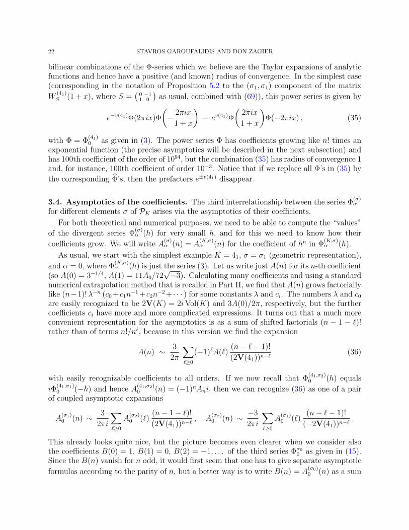
22 STAVROS GAROUFALIDIS AND DON ZAGIER
bilinear combinations of the Φ-series which we believe are the Taylor expansions of analyticfunctions and hence have a positive (and known) radius of convergence. In the simplest case(corresponding in the notation of Proposition 5.2 to the (σ1, σ1) component of the matrix
W(41)S (1 + x), where S =
(0 −11 0
)as usual, combined with (69)), this power series is given by
e−v(41)Φ(2πix)Φ
(− 2πix
1 + x
)− ev(41)Φ
(2πix
1 + x
)Φ(−2πix) , (35)
with Φ = Φ(41)0 as given in (3). The power series Φ has coefficients growing like n! times an
exponential function (the precise asymptotics will be described in the next subsection) andhas 100th coefficient of the order of 1094, but the combination (35) has radius of convergence 1and, for instance, 100th coefficient of order 10−3. Notice that if we replace all Φ’s in (35) by
the corresponding Φ’s, then the prefactors e±v(41) disappear.
3.4. Asymptotics of the coefficients. The third interrelationship between the series Φ(σ)α
for different elements σ of PK arises via the asymptotics of their coefficients.
For both theoretical and numerical purposes, we need to be able to compute the “values”
of the divergent series Φ(σ)α (h) for very small h, and for this we need to know how their
coefficients grow. We will write A(σ)α (n) = A
(K,σ)α (n) for the coefficient of hn in Φ
(K,σ)α (h).
As usual, we start with the simplest example K = 41, σ = σ1 (geometric representation),
and α = 0, where Φ(K,σ)α (h) is just the series (3). Let us write just A(n) for its n-th coefficient
(so A(0) = 3−1/4, A(1) = 11A0/72√−3). Calculating many coefficients and using a standard
numerical extrapolation method that is recalled in Part II, we find that A(n) grows factoriallylike (n−1)!λ−n (c0 +c1n
−1 +c2n−2 + · · · ) for some constants λ and ci. The numbers λ and c0
are easily recognized to be 2V(K) = 2iVol(K) and 3A(0)/2π, respectively, but the furthercoefficients ci have more and more complicated expressions. It turns out that a much moreconvenient representation for the asymptotics is as a sum of shifted factorials (n − 1 − `)!rather than of terms n!/n`, because in this version we find the expansion
A(n) ∼ 3
2π
∑`≥0
(−1)`A(`)(n− `− 1)!
(2V(41))n−`(36)
with easily recognizable coefficients to all orders. If we now recall that Φ(41,σ2)0 (h) equals
iΦ(41,σ1)0 (−h) and hence A
(41,σ2)0 (n) = (−1)nAni, then we can recognize (36) as one of a pair
of coupled asymptotic expansions
A(σ1)0 (n) ∼ 3
2πi
∑`≥0
A(σ2)0 (`)
(n− 1− `)!(2V(41))n−`
, A(σ2)0 (n) ∼ −3
2πi
∑`≥0
A(σ1)0 (`)
(n− `− 1)!
(−2V(41))n−`.
This already looks quite nice, but the picture becomes even clearer when we consider alsothe coefficients B(0) = 1, B(1) = 0, B(2) = −1, . . . of the third series Φσ0
0 as given in (15).Since the B(n) vanish for n odd, it would first seem that one has to give separate asymptotic
formulas according to the parity of n, but a better way is to write B(n) = A(σ0)0 (n) as a sum
KNOTS, PERTURBATIVE SERIES AND QUANTUM MODULARITY 23
of two asymptotic expansions labelled by the two other elements σ1 and σ2 of PK :
B(n) ∼√
2π∑`≥0
A(σ1)0 (`)
Γ(n− `+ 32)
(−V(41))n−`+3/2−√
2π∑`≥0
A(σ2)0 (`)
Γ(n− `+ 32)
V(41)n−`+3/2. (37)
Here we observe that the expressions 2V(41), −2V(41), −V(41) and V(41) occurring in thedenominators of the last two formulas can be written in a uniform way as V(σ1) −V(σ2),V(σ2)−V(σ1), V(σ0)−V(σ1) and V(σ0)−V(σ2), respectively. Exactly analogous asymptotic
statements turn out to hold for the coefficients of the series Φ(41,σ)α also for α 6= 0, with the
same coefficients, leading for this knot to the uniform conjectural statement
A(K,σ)α (n) ∼ (2π)κσ−1
∑σ′ 6=σ
MK(σ, σ′)∑`≥0
A(σ′)α (`)
Γ(n− `+ κσ)(V(σ)−V(σ′)
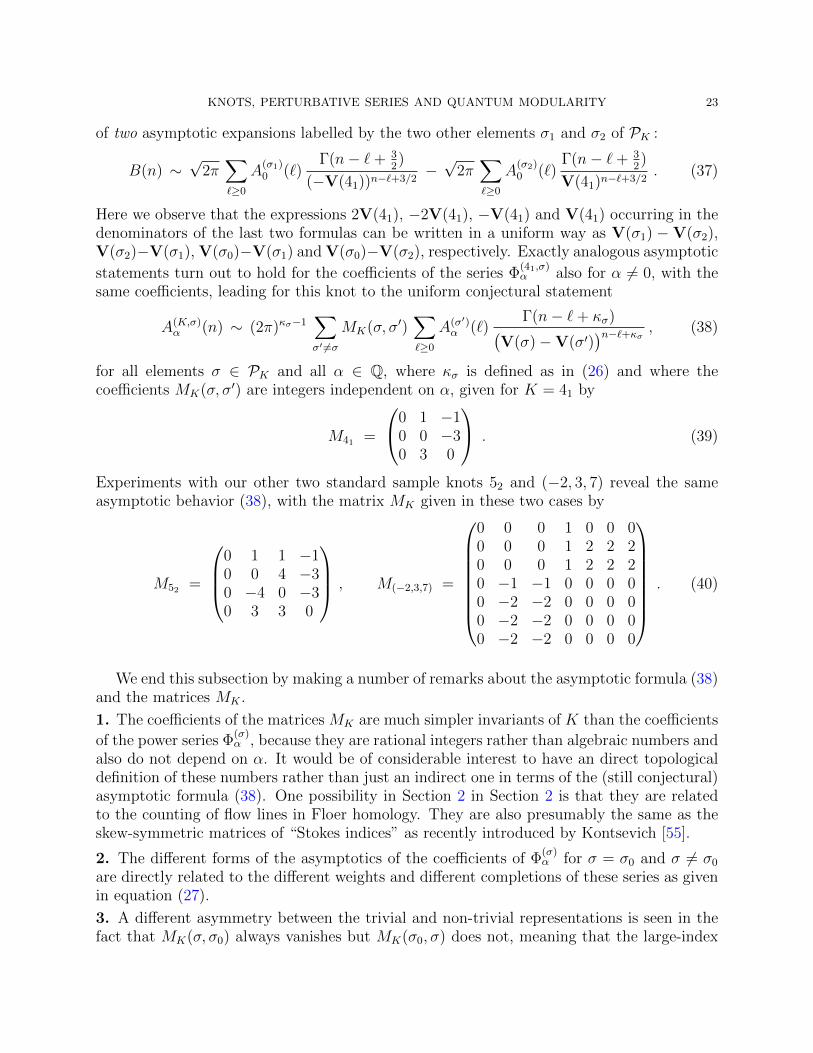
)n−`+κσ , (38)
for all elements σ ∈ PK and all α ∈ Q, where κσ is defined as in (26) and where thecoefficients MK(σ, σ′) are integers independent on α, given for K = 41 by
M41 =
0 1 −10 0 −30 3 0
. (39)
Experiments with our other two standard sample knots 52 and (−2, 3, 7) reveal the sameasymptotic behavior (38), with the matrix MK given in these two cases by
M52 =
0 1 1 −10 0 4 −30 −4 0 −30 3 3 0
, M(−2,3,7) =
0 0 0 1 0 0 00 0 0 1 2 2 20 0 0 1 2 2 20 −1 −1 0 0 0 00 −2 −2 0 0 0 00 −2 −2 0 0 0 00 −2 −2 0 0 0 0
. (40)
We end this subsection by making a number of remarks about the asymptotic formula (38)and the matrices MK .
1. The coefficients of the matrices MK are much simpler invariants of K than the coefficients
of the power series Φ(σ)α , because they are rational integers rather than algebraic numbers and
also do not depend on α. It would be of considerable interest to have an direct topologicaldefinition of these numbers rather than just an indirect one in terms of the (still conjectural)asymptotic formula (38). One possibility in Section 2 in Section 2 is that they are relatedto the counting of flow lines in Floer homology. They are also presumably the same as theskew-symmetric matrices of “Stokes indices” as recently introduced by Kontsevich [55].
2. The different forms of the asymptotics of the coefficients of Φ(σ)α for σ = σ0 and σ 6= σ0
are directly related to the different weights and different completions of these series as givenin equation (27).
3. A different asymmetry between the trivial and non-trivial representations is seen in thefact that MK(σ, σ0) always vanishes but MK(σ0, σ) does not, meaning that the large-index
24 STAVROS GAROUFALIDIS AND DON ZAGIER
coefficients of the Φ(σ0) series “see” the small-index coefficients of the Φσ series for σ 6= σ0
but not vice versa. It is interesting to note that similar “one-way phenomenon” regardingthe matrices appearing in recent work of Gukov et al [46, 45].
4. In all three examples given above, we further observe that apart from their first col-umn, which vanishes, and first row, which does not, the matrices MK are skew-symmetric,i.e., MK(σ, σ′) = −MK(σ′, σ) for σ, σ′ 6= σ0. This phenomenon, which we expect to hold forall knots, will be shown below to be a formal consequence of the quadratic relation (34).
5. We also observe that the lower 4× 4 block of the matrix M(−2,3,7) vanishes identically. Inview of the numbering of the indices, this means that MK(σ, σ′) vanishes whenever σ andσ′ are both real and distinct from σ0. This in fact holds for all knots and is a special caseof the more general identity MK(σ, σ′) = −MK(σ, σ′) for all σ, σ′ 6= σ0, which we can proveeasily (assuming that the expansion (38) is correct) simply by taking the complex conjugate
of (38) and noting that V(σ) and A(σ)α (n) are the complex conjugates of V(σ) and A
(σ)−α(n),
respectively (and, of course, that the coefficients of MK are real). The minus sign arises fromthe pure imaginary prefactor (2πi)−1 in (38).
6. A corollary of (38) is the growth estimate
A(σ)σ (n) = O
(nκσ−1n! ∆(σ)−n
), (41)
where
∆(σ) = ∆(K, σ) = minMK(σ,σ′) 6=0
∣∣V(σ)−V(σ′)∣∣ . (42)
This estimate will be important for the optimal truncation that is used in the next sectionand discussed in more detail in Section 10 and in [40].
7. We should also mention that there is still some sign ambiguity in the definition of thematrix MK . At the moment, even assuming the validity of the various conjectures presented
in the next two sections, we can only normalize the power series Φ(σ)σ (h) up to the ambiguity
of a sign εσ ∈ {±1} independent of α but depending on σ, and making this change wouldmultiply MK(σ, σ′) by εσεσ′ (which would not affect either of the properties mentioned in 3.and 4. above). Similarly, when σ = σ0 the formula defining MK(σ, σ′) has an inherentambiguity coming from the choice of sign of square-root of Vσ − Vσ′ = −Vσ′ in (38) (onlyin the first term; the choices for the other terms are then determined in the obvious way),so that each of the matrix entries MK(σ0, σ
′) is actually only well defined up to sign. Ofcourse, it is possible that there is some canonical way to normalize everything to eliminatethese ambiguities, but we do not yet know how to do this.
8. Actually, however, there is a problem with all of these statements that we have glossedover so far but that does need to be addressed. This is that the right-hand side of (38)does not really make sense as it stands, since the terms on the right-hand side are given bydivergent series and hence can be computed only up to some level of precision, but at thesame time have exponentially different orders of growth, so that it is not a priori clear whatit means to add them. In the case of 41 we did not see this problem, because there is onlyone term in (38). This point will be discussed briefly in Section 10.2 and in detail in [40].
KNOTS, PERTURBATIVE SERIES AND QUANTUM MODULARITY 25
4. Refining the Quantum Modularity Conjecture
In this section we will show how one can go beyond the original QMC as described in Section 1or its generalization as described in Subsection 3.1. We will present this via a series ofsuccessive refinements, each one found experimentally and building on its predecessors.
4.1. Improving the Quantum Modularity Conjecture: optimal truncation. The
QMC in its original form says that J (K)(−1/X) agrees with X3/2 J (K)(X) Φ(K)0 (2πi/X) to
all orders in 1/X as X tends to infinity with fixed denominator, with a similar statementwhen −1/X is replaced by aX+b
cX+dfor any
(a bc d
)∈ SL2(Z). A natural question is whether we
can do better than this and obtain an asymptotic estimate, or even a precise asymptoticformula, for the difference of these two expressions. At first sight this seems to makes no
sense, since Φ(K)0 (h) (or more generally Φ
(K)a/c (h)) is given in terms of a divergent power series
that a priori does not have a numerical value but rather gives only an approximation up to
any given order in h. But we can remedy this by replacing the series Φ(h) = Φ(K)0 (h) or
Φ(K)a/c (h) by its “optimal truncation” Φ(h)opt obtained by truncating the divergent infinite
series at the value of N (depending on h) where the terms of this series become smallest inabsolute value, a little like what is done in physics when for instance the magnetic momentof the electron is computed to high accuracy by truncating a divergent sum of Feynmanintegrals at a suitably small term. If Φ(h) =
∑Anh
n with An growing like n!/Bn for some
complex number B, then this “naive optimal truncation” is given by∑N
n=0 Anhn with N
chosen near to |B/h|. Then the first term neglected, and hence also the expected error, is ofthe order of magnitude of e−N , so we have a way to define Φ(h) up to an exponentially smallerror rather than only up to fixed powers of h. Of course, to get a completely well-definedfunction Φ(h)opt we would have to fix a prescription for choosing N , say as the floor or ceilingor nearest integer to |B/h| (and perhaps also dividing by 2 the last term retained), but sincethe terms with n ≈ |B/h| are all very small the specific choice is not important and we willdo better later anyway.
Using the description of the asymptotics of the coefficients of the series Φ(K,σ)α (h) given in
Section 3.4 above, we can compute their optimal truncations explicitly. Starting as usual withthe simplest example K = 41 and α = 0 (and also Φ = Φ(σ1) = Φ(41,σ1), the series occurringin the QMC), we have from (36) the estimate An = O(n!/(2V )n) with V = Vol(41) =2.02988 · · · , so the optimal truncation occurs for N near 2V/|h|. The expected error in Φ(h)for h = 2πi/X is therefore of the order of e−2v(41)X , with v(41) = V/2π = 0.32306 · · · , and
since the completed function Φ(h) = eV/hΦ(h) grows like ev(41)X , this means that not only the
relative but even the absolute expected error in Φ(h)opt is exponentially small in this case. Asa numerical example, we consider the value X = 100. The Kashaev invariant 〈41〉100, whichwe can compute to arbitrary precision from (14) with q = ζ100, has the approximate value
81985188380512462.9310054954341, while the corresponding value 1003/2 Φ(
2πi100
)opt(obtained
in this case by retaining the first 66 coefficients of the divergent series) has the numericalvalue 81985188380512461.9269943535808 with an expected error of the order of 10−12. We seeimmediately that these two numbers are not equal within the accuracy of the computation,so that the most obvious first guess for a more precise version of the QMC is not true. But
26 STAVROS GAROUFALIDIS AND DON ZAGIER
when we look at the difference of these two numbers we find the numerical value⟨41
⟩100− 1003/2 Φ
(2πi
100
)opt ≈ 1.00401114185 ,
which is very close to 1. Repeating the experiment for other large integral values of X, wefind that this difference has the asymptotic expansion 1− h2 + 47
12h4 + · · · (with h = 2πi/X
as before), which we recognize easily as the power series Φ(41,σ0)(h) as given in (15), and anumerical computation shows that indeed the optimal truncation of that series at h = 2πi
100has
precisely the same value 1.00401114185, to the same precision. Repeating the calculationswith other integral and non-integral values of X and also for J (41)(γX) for matrices γ ∈SL2(Z) other than
(0 −11 0
), we find the same behavior in all cases, leading to the conjectural
asymptotic formula
(cX + d)−3/2 J (41)(aX + b
cX + d
)?≈ J (41)(X) Φ(41,σ1)
( 2πi
c(cX + d)
)+ Φ(41,σ0)
( 2πi
c(cX + d)
)(43)
for any matrix γ =(a bc d
)∈ SL2(Z) and for X → ∞ with fixed (or bounded) denominator,
with the coefficient of the second series Φ(41,σ0) being 1 for all X and γ.
Here the natural question arises whether one can improve the precision of (43) even
further by adding to the right-hand side a third term involving Φ(41,σ2), the last of the threecompleted series for the 41 knot. But for the moment we can’t even make sense of this since
the intrinsic error in the optimal-truncation values of both Φ(41,σ1)(h) and Φ(41,σ0)(h) hasexponential decay of the order of e−v(K)X (for the first function because it grows like e+v(K)X
and has a relative error e−2v(K)X , as we have already seen, and for the second because itgrows only like a power of X but has a larger relative error e−v(K)X by virtue of (37)). This
is the same as the order of growth of the third function Φ(41,σ2)(h), so that dividing the
difference of the left- and right-hand sides of (43) by Φ(41,σ2)(h), with all Φ-series definedby optimal truncation, would give meaningless values. We will return to this problem inSubsection 4.3 below. Before doing that, however, we first look at two other knots for whicha new phenomenon appears that is not visible for 41 .
4.2. New elements of the Habiro ring. For the knot K = 52 the set PK has fourelements: the Habiro one, the geometric and antigeometric ones, and the one correspondingto the real embedding of the cubic field FK = Q(ξ). However, it has only three distinct realvolumes: the geometric volume =V(σ1) = Vol(K) (with the numerical value 2.82812 · · · ),the anti-geometric volume =V(σ2) = −Vol(K), and 0 for both σ = σ0 and σ = σ3, andconsequently only three distinct orders of growth (one exponentially large, one exponentially
small, and two of polynomial growth) of the corresponding Φ-functions Φ(K,σ)(h). (Forsimplicity we concentrate for the moment only on α = 0 and omit it from the notations.)This means that in the analogue of (43) there is only one term that is too small to be seennumerically when we replace the Φ-series by their optimal truncation, so that here one canhope to see three distinct terms on the right. To test this, we take the same values N = 100,h = 2πi/N as before. Then J (K)
(− 1N
)is of the order of magnitude of 1022 and the difference
N−3/2J (K)(− 1N
) − Φ(K,σ1)(h)opt − Φ(K,σ0)
(h)opt
is of the order of 1 just as before, but now
when we divide this difference by Φ(K,σ3)(h)opt
we obtain 2 + (1.22− 5.23i) · 10−9, strongly
KNOTS, PERTURBATIVE SERIES AND QUANTUM MODULARITY 27
suggesting that the limiting value of this difference as X tends to infinity through integersexists and is equal to 2. Further experiments for non-integral values of X and for othermatrices γ =
(a bc d
)then lead to the new conjectural asymptotic statement
(cX + d)−3/2 J (52)(aX + b
cX + d
)(44)
?≈ J (52)(X) Φ
(52,σ1)a/c
( 2πi
c(cX + d)
)+ Φ
(52,σ0)a/c
( 2πi
c(cX + d)
)+ Q(52)(X) Φ
(52,σ3)a/c
( 2πi
c(cX + d)
)for all γ and all X tending to infinity with bounded denominator, where Q(52)(x) (which is atemporary notation, only for this knot) is a function that is independent of γ but that, unlike
the constant coefficient 1 of the Habiro term Φ(K,σ0)(h), is not independent of x. Instead,Q(52)(x) is numerically found to be a periodic function of period 1 taking on simple algebraicvalues, the first few being
Q(52)(0) = 2, Q(52)(12) = 8, Q(52)(±1
3) = 37±3
√−3
2, Q(52)(±1
4) = 29± 13i .
Looking at more values (specifically, for all x with denominator up to 200), we find thatQ(52)(x) belongs to Z[e(x)] and is Galois-invariant, so we can write it as Q(52)(e(x)) whereQ(52)(q) is an element of Z[q] for every root of unity q, the first values being given by
Ord(q) 1 2 3 4 5 6
Q(52)(q) 2 8 20 + 3q 29 + 13q 69 + 27q + 37q2 + 2q3 −46 + 69q
This suggests that q 7→ Q(52)(q) might be an element of the Habiro ringH defined in (12), just
as we know is the case for the coefficient J (52)(X) of the first Φ-term in (44). This hypothesiscan be tested numerically, because a well-known property of any element Q ∈ H (originallyobserved by Ohtsuki [61] in the context of the WRT-invariants of integer homology sphereseven before the Habiro ring had been formalized) is that it satisfies an infinite numberof congruences, the simplest of which is that Q(ζp) for every prime number p should becongruent modulo p to c0 + c1πp + c2π
2p + · · · + cp−2π
p−2p , where πp = ζp − 1 is the prime
dividing p in Q(ζp) and where the ci are rational integers independent of p. This means inour case that the coefficient of xi in the polynomial Qp(1 + x) ∈ Z[x] should be congruentmodulo p to a fixed integer ci ∈ Z for all primes p > i+1, and testing this for the numericallyobtained polynomials Qn, we find that it is indeed true, with Qp(ζp) ≡ Oh(πp) (mod p) fora power series Oh(x) ∈ Z[[x]] beginning
Oh(x) = 2− 3x+ 8x2 − 28x3 + 120x4 − 614x5 + 3669x6 − 25125x7 + O(x8) . (45)
In fact, later we were able to guess an explicit formula, given below in Section 7.1, that ismanifestly in the Habiro ring and that reproduces the values of the polynomials Qn(q) andpower series Oh(x) as given above. But in many other cases, including the (−2, 3, 7) knotdiscussed below, we cannot give even conjectural explicit formulas of the required kind, andin such cases it is important to be able to have a numerical test of the Habiro-ness of aperiodic function.
28 STAVROS GAROUFALIDIS AND DON ZAGIER
Notice that the right-hand side of (44) contains only three of the four completed power
series Φ52,σa/c . Just as for the 41 knot, this is not because the last one isn’t really there, but
because our approximate evaluations are not accurate enough at this point to detect theremaining term, which is exponentially small. We will correct this in Section 4.3.
We were able to carry out similar calculations for the (−2, 3, 7) pretzel knot, though thenumerical analysis required here was much more arduous due to the larger number of seriesinvolved. Recall that this knot has rank 6, so that PK contains seven elements. What makesthe calculation feasible at all is that five of these seven elements are real (the Habiro oneand the ones corresponding to the real embedding of Q(ξ) and to all three embeddings of
Q(η)), so that only one of the seven Φ-functions is exponentially small and hence invisiblewith optimal truncation. (Actually, the fact that the other terms apart from the geometricone are of the order of 1 is not quite enough: one also has to verify by using the formulasof 3.4 and the numerical values of the complex volumes v(K, σi) that the absolute error made
in calculating the exponentially large dominant term Φ(K,σ1)(h) using optimal truncation isexponentially small.) We find a formula exactly analogous to (44), but now with six termson the right, namely
(cX + d)−3/2 J (−2,3,7)(aX + b
cX + d
)?≈
∑0≤j≤6j 6=2
Q(−2,3,7)j (X) Φ
((−2,3,7),σj)
a/c
( 2πi
c(cX + d)
), (46)
where j = 2 is omitted for the same reason as in (44) (viz., that the corresponding term is
too small to see at this stage) and where Q(−2,3,7)1 (x) = J (−2,3,7)(x), and Q
(−2,3,7)0 (x) ≡ 1, and
the four new periodic functions Q(−2,3,7)j (x) = Q(−2,3,7)
j (e(x)) take values in Z[e(x)] just asbefore, the first values (for j 6= 0, 2) being
Ord(q) 1 2 3 4 5 6
Q(−2,3,7)1 (q) 1 1 −5 + 6q 17− 8q −21− 27q − 5q2 + 4q3 −107 + 108q
Q(−2,3,7)3 (q) −4 −12 −15− 10q −16− 2q −36− 20q − 29q2 − 24q3 23 + 14q
Q(−2,3,7)4 (q) 2 −10 −16− 12q −46q −8− 44q − 38q2 − 48q3 116− 24q
Q(−2,3,7)5 (q) −2 −6 −14− 6q 8− 10q 32q − 4q2 − 10q3 −82 + 122q
Q(−2,3,7)6 (q) 2 2 4− 8q 10− 12q −4− 36q − 44q2 − 34q3 136− 16q
Just as with the 52 knot, we can verify the Ohtsuki property for these functions to a largenumber of terms and thus convince ourselves that each one belongs to the Habiro ring, eventhough in this case we do not know an explicit formula that makes this property manifest.
4.3. Smoothed optimal truncation. We already mentioned at the end of Subsection 4.1
that it would be natural to expect a third term in (43) involving the missing Φ-function
Φ(K,σ2)(h), and the same applies even more strikingly to the two knots discussed in Subsec-tion 4.2, where we were obliged to omit the σ2-term in both (44) and (46) because it would
have been absorbed in the error terms of the other Φ’s and hence could not be seen numer-ically if these values were defined by naive optimal truncation. However, there is a moreprecise way of turning the divergent series Φ(h) = Φσ
α(h) into functions that are defined up
KNOTS, PERTURBATIVE SERIES AND QUANTUM MODULARITY 29
to exponentially rather than merely polynomially small errors, but with a much better ex-ponent than before, by replacing the naive optimal truncation Φ(h)opt by a smoothed versionΦ(h)sm. The details of the procedure to do this are somewhat complicated and play no rolefor the story we are telling here, so will be given in detail in a separate publication [40] anddescribed briefly in Section 10.2, the only important point here being that the improvementis sufficiently good, at least for our three standard knots, that we can unambiguously identify
the periodic coefficients of the missing Φ-terms.
We start as usual with the knot K = 41 and the series Φ(h) = Φ(σ1)0 (h) whose initial
terms are given in (3). In 4.1 we considered X = 100, h = 2πiX
and saw that the number
1003/2 Φ(h)opt ≈ 8.195 × 10¹⁶ had an error of the order of 10−12, which was more than
sufficient to identify its difference with⟨41
⟩100
unambiguously as Φ(σ0)(h) but not enough to
see a possible contribution from the much smaller Φ(σ2)(h). If we replace optimal by smooth
truncation, then the error in Φ(h) decreases from (approximately) 10−15 to 10−44 and the
error in Φ(σ0)(h) from 10−15 to 10−42. We can therefore compute the difference of the left-and right-hand sides of (43) (for X = 100, γ = S) to 42 digits, finding that it vanishes,
and since the remaining Φ-value Φ(σ2)(h) has the much larger order of 10−14, we see thatthis quantity, if it occurs at all, must have coefficient 0. But when we replace X = 100 by
10013, we find that the difference X−3/2 J(−1/X) − J(1
3)Φ(σ1)(h)sm − Φ(σ0)
(h)sm
no longer
vanishes but instead is equal to Φ(σ2)(h)sm
times −1.732050807568877293527446341 i, which
coincides to this accuracy with −√−3. Doing the same for other large values of X with
small denominators and other γ, we find that (43) with all Φ-values interpreted by smoothrather than optimal truncation can be improved to
(cX + d)−3/2 J (41)(aX + b
cX + d
)?≈
2∑j=0
Q(41)j (X) Φ(41,σj)
( 2πi
c(cX + d)
)(47)
where, just as for the (−2, 3, 7) pretzel knot, Q(41)0 (x) = 1, Q
(41)1 (X) = J (41)(x) and Q
(41)2 is
a 1-periodic functions, the notations in each case being a shorthand for Q(41)σj . The first few
values of the periodic functions Q(41)i (x) = Q(41)
i (e(x)) for i = 1 and 2 are given by
Ord(q) 1 2 3 4 5 6
Q(41)1 (q) 1 5 13 27 44− 4q2 − 4q3 89
2Q(41)2 (q) 0 0 −2− 4q −14q −15− 30q − 22q2 − 8q3 46− 92q
Just as with the functions Q(52)(x) and Q(−2,3,7)i (x) (i = 3, 4, 5, 6) found for the 52 and
(−2, 3, 7) knots in the previous subsection, the function Q(41)2 (whose values we found by
the numerical procedure just outlined for all x with denominators up to 200), multipliedby 2, turned out to always belong to Z[e(x)] and to satisfy all of the necessary Ohtsuki-typecongruences near 0 and 1/2 required for it to be an element of the Habiro ring. In thiscase, following a tip by Campbell Wheeler, we were actually able to guess a formula thatreproduced all of the numerically found values and (after multiplication by 2) was visibly in
30 STAVROS GAROUFALIDIS AND DON ZAGIER
the Habiro ring, namely the following simple variant of equation (14):
Q(41)2 (q) =
1
2
∞∑n=0
(qn+1 − q−n−1) (q−1; q−1)n (q; q)n . (48)
When we recompute the examples of Subsection 4.2 with smooth rather than optimal
truncation, the situation is exactly similar and we are able to add a Φ(K,σ2)α (h) term to the
right-hand sides of both (44) and (46), obtaining for both knots a conjectural approximateformula of the form
(cx+ d)−3/2 J (K)(aX + b
cX + d
)?≈
∑σ∈PK
Q(K)σ (X) Φ
(K,σ)a/c
( 2πi
c(cX + d)
), (49)
where Q(K)σ0 (x) = 1 and Q
(K)σ1 (x) = J (K)(x). In Sections 7.1 and 9 we give more information
about these numbers including a formula for Q(52)σ2 (x) as an element of the Habiro ring.
4.4. Strengthening the Generalized Quantum Modularity Conjecture. So far wehave generalized the original Quantum Modularity Conjecture (6) in two very different ways:in Subsection 3.1 we extended it from the Kashaev invariant J = J (σ0) to the functions definedin (19), and in the last three subsections we refined it by adding additional terms of lowerorder to the right-hand side. Not surprisingly, these two can be combined, but with somenew aspects.
If we repeat the calculations described in the previous subsection (using smooth truncationfor all the Φ-series occurring) but with the function J (K) = J (K,σ0) replaced by the functiondefined in (19) with σ 6= σ0, then instead of (49) we find
e−v(σ)λγ(X) J (K,σ)(aX + b
cX + d
)?≈
∑σ′∈PK
J (K,σ,σ′)(X) Φ(K,σ′)a/c
( 2πi
c(cX + d)
), (50)
where J (K,σ,σ′) are periodic functions on Q with J (K,σ,σ1)(x) ≡ 1 reproducing the first termin (49). There are, however, three main differences with that equation. The first is thatthe automorphy factor (cX + d)3/2 does not occur. The second is that the Habiro power
series Φ(K,σ0)a/c , which in (49) always had the coefficient 1, now does not occur at all. The
third is that the new functions J (K,σ,σ′)(x) (or rather the corresponding functions Q(q),where q = e(x)) are now not in the Habiro ring, but are still Q-valued and have various“Habiro-like” properties including the following:
• J (K,σ,σ′)(x) for x ∈ Q/Z is the constant term of a power series Φ(K,σ,σ′)x (h) lying in
the same space as the power series Φ(K,σ)x (h), as discussed briefly after eq. (7) and in
more detail in Section 9, i.e., it belongs to µ δ−1/2 m√ε Fσ(ζm)[[h]] with the same root
of unity µ, the same element δσ of F×σ , the same set S of primes of Fσ (independent
of x) and the same S-unit ε = εx of Fσ(ζm) as for Φ(K,σ)x (h).
• one can interpret Φ(K,σ,σ′)x (h) as Q(e(x)e−h) where Q is an element of a Habiro ring
HFσ generalizing the ordinary Habiro ring H = HQ whose definition and arithmeticproperties will be discussed in a planned joint paper with Peter Scholze [35]. In
KNOTS, PERTURBATIVE SERIES AND QUANTUM MODULARITY 31
particular, for primes p that split completely in Fσ, there are congruence propertiesmodulo p relating, for instance, the first p coefficients of Q(e−h) to the value of Q(ζp).
We can write equation (50) more uniformly by allowing the case of σ = σ0, but remem-bering that there is then an automorphy factor (cX + d)−3/2 that is not present for σ ∈ PK .Then all of the formulas found so far can be collected into a single conjectural formula
e−v(σ)λγ(X) (cX + d)−κ(σ) J (K,σ)(aX + b
cX + d
)?≈
∑σ′∈PK
J (K,σ,σ′)(X) Φ(K,σ′)a/c
( 2πi
c(cX + d)
)(51)
valid for all γ =(a bc d
)∈ SL2(Z) and all σ ∈ PK for X → ∞ with bounded denominator,
where J (K,σ,σ′) are periodic functions belonging to a generalized Habiro ring and satisfying
J (K,σ,σ0) = δσ,σ0 and J (K,σ0,σ) = Q(K)σ (as introduced in the previous section), with the weight
κσ and the multiplier λγ(X) defined as in (24) and (26).
As a concrete illustration of the refined QMC (51) we take once again the figure 8 knotwith σ = σ1. Here, (51) involves three terms σ′ = σ0, σ1, σ2, with two of the three coefficientsalready known (the first vanishes and the second is J (41,σ1)(X)) but with the third one beinga new periodic function on Q given explicitly by
J (41,σ1,σ2)(x) = i4√
3
2√c
∑Zc = ζ6
(Zq − Z−1q−1)c∏j=1
∣∣1 − qjZ∣∣2j/c (c = den(x), q = e(x)) ,
(52)
which is related to the function given in (20) in exactly the same way as Q(41)σ2 (x) and J (41)(x)
are related by (48) and (14). Likewise, the refined QMC (51) for 41 and for σ = σ2 leads tothe periodic function J (41,σ2,σ2)(x) = −i J (41,σ1,σ2)(−x). We also find the bilinear identity
J (41,σ1)(x) J (41,σ2)(x) − J (41,σ1,σ2)(x) J (41,σ2,σ1)(x) = 1 (53)
for all x ∈ Q/Z. This identity will be generalized to all knots in Section 5.
4.5. The Refined Quantum Modularity Conjecture. The refinement of the QuantumModularity Conjecture that we have obtained so far, equation (51), has two noteworthyaspects. One is that, although we find new collections of “Habiro-like” functions J (σ,σ′) forthe asymptotic expansion as X →∞ of the functions J (σ0,σ)(γX) for different σ ∈ PK (herewe continue the practice of omitting the knot from all notations when it is not varying),
these arise as coefficients of the same completed formal power series Φ(σ′)(h) as we foundfor the initial Galois-extended Kashaev invariant J (σ0). The other is that among the newcoefficients J (K,σ,σ′), the subset corresponding to σ′ = σ1 coincides precisely with the set offunctions J (σ) whose asymptotic behavior near fixed rational points is being studied. It istherefore natural to ask whether the functions J (K,σ,σ′) for σ′ different from σ1 also have aquantum modularity property, and if so, what new power series are involved. In this finalsubsection we will study both questions and give our (nearly) final version of the QMC.
As usual, we look first at the 41 knot. Here, as well as the three periodic functionsJ (σ0,σ1)(x) := J(x) and Jσ0,σ1(x) := J (σ1) and J (σ0,σ2) := J (σ2) we had studied earlier, wefound two new periodic functions J (σ1,σ2)(x) and Jσ2,σ2)(x), given explicitly by formulas (52).
32 STAVROS GAROUFALIDIS AND DON ZAGIER
If we look numerically at the asymptotics of both functions with x = −1/X for X → ∞with bounded denominator, we find
X−3/2J (σ0,σ2)(− 1
X
)∼ J(X)(σ0,σ1) Ψ(1)
(2πi
X
),
e−v(σ1)λS(X) J (σ1,σ2)(− 1
X
)∼ J (σ1,σ1)(X) Ψ(1)
(2πi
X
)with the same completed power series
Ψ(1)(h) = eV(41)/h Ψ(1)(h), Ψ(1)(h) =i 4√
3
2
(1 − 37
72√−3
h − 1511
2(72√−3)2
h2 + · · ·)
in both cases. Based on the analogy with the asymptotics of the functions J (σ1,σ1)(−1/X)as given in (47), we would now expect the more accurate approximations
X−3/2J (σ0,σ2)(−1/X) ≈ Ψ(0)(2πi/X) + J (σ0,σ1)(X) Ψ(1)(2πi/X) + J (σ0,σ2)(X) Ψ(2)(2πi/X) ,
e−v(σ1)λS(X)J (σ1,σ2)(−1/X) ≈ J (σ1,σ1)(X) Ψ(1)(2πi/X) + J (σ1,σ2)(X) Ψ(2)(2πi/X) , (54)
e−v(σ2)λS(X)J (σ2,σ2)(−1/X) ≈ J (σ2,σ1)(X) Ψ(1)(2πi/X) + J (σ2,σ2)(X) Ψ(2)(2πi/X) ,
where Ψ(2)(h) is the completed series e−V(41)/h Ψ(2)(h) with Ψ(2)(h) = −iΨ(1)(−h) and where
Ψ(0)(h) is the completed series (h/2πi)3/2 Φ(0)(h) (cf. (18)) with
Φ(0)(h) = −h +11
6h3 − 1261
120h5 +
611771
5040h7 − · · ·
the power series in hQ[[h2]] obtained by replacing q = e(X) by q = e−h in formula (48),as well of course as similar formulas for J (σ,σ′)(γX) for other matrices γ =
(a bc d
)in SL2(Z)
with the completed power series Ψ(j)(h) replaced by suitable new completed power series
Ψ(j)a/c(h) = eV(σj)/ch(h/2πi)κ(σj)Ψ
(j)a/c(h) but with the same periodic coefficients.
To test (54) or its generalizations to other γ ∈ SL2(Z) directly we would need to find many
terms of the power series Ψ(j)α (h) and carry out the smoothed optimal truncation as described
earlier in this section, because the different exponential growths of their completions wouldmean that the contributions with j 6= 1 would not be numerically visible at the level of mereformal power series. This could be done, but an easier test of the prediction is to take linear
combinations of the first two or last two lines in (54) to eliminate the dominant Ψ(1)-term.This (together with (53)) produces the two new asymptotic predictions
X−3/2 J (σ1,σ1)(X) J (σ0,σ2)(− 1X
) − e−v(σ1)λS(X)J (σ0,σ1)(X) J (σ1,σ2)(− 1X
) ≈ J (σ1,σ1)(X) Ψ(0)(2πiX
) ,
e−v(σ1)λS(X)J (σ2,σ1)(X) J (σ1,σ2)(− 1X
) − e−v(σ2)λS(X)J (σ1,σ1)(X) J (σ2,σ2)(− 1X
) ≈ Ψ(2)(2πiX
) ,
both of which can be tested directly since they do not involve functions of different ordersof growth on the right, and both of which we confirmed numerically to very high precision.We omit the details, having given more than enough descriptions of analogous numericalcalculations in this section already.
KNOTS, PERTURBATIVE SERIES AND QUANTUM MODULARITY 33
Generalizing the above discussion to other knots, we find as our nearly-final version ofthe QMC the asymptotic statement
(cX + d)−κ(σ) e−v(σ)λγ(X) J (K,σ,σ′)(aX + b
cX + d
)?≈
∑σ′′ ∈PK
J (K,σ,σ′′)(X) Φ(K,σ′′,σ′)a/c
( 2πi
c(cX + d)
)for X ∈ Q tending to infinity with bounded denominator and for every
(a bc d
)∈ SL2(Z)
with c > 0, where the functions J (K,σ,σ′) are the “Habiro-like” functions that we found in
Section 4.4, given as the constant terms of certain power series Φ(K,σ,σ′)α (h) ∈ Q[[h]], and
where Φ(K,σ,σ′)α (h) are the completions defined by
Φ(K,σ,σ′)α (h) = (ch/2πi)κ(σ) eV(σ)/c2h Φ(K,σ,σ′)
α (h)(σ, σ′ ∈ PK
). (55)
To get the final version, we upgrade this statement about constant terms to a statementabout the full (completed) power series in the same way as we did in 3.2, obtaining:
Refined Quantum Modularity Conjecture (RQMC): For fixed γ =(a bc d
)∈ SL2(Z)
with c > 0, we have
Φ(K,σ,σ′)γX (h∗)
?≈ (cx+ d)κ(σ)
∑σ′′ ∈PK
Φ(K,σ,σ′′)X (h) Φ
(K,σ′′,σ′)a/c
( 2πi
c(cx+ d)
)(56)
to all orders in 1/X as X ∈ Q tending to +∞ with bounded denominator, where x = X − ~and h∗ = h/(cx+ d)(cX + d).
We end this section by observing that the two versions of the Refined Quantum ModularityConjecture that we just stated can both be writte more succinctly in matrix form as
J(K)(γX) ≈ jγ(X) J(K)(X) Φ(K)a/c
( 2πi
c(cX + d)
)(57)
and
Φ(K)γX (h∗)
?≈ jγ(x)−1 Φ
(K)X (h) Φ
(K)a/c
( 2πi
c(cx+ d)
). (58)
as X →∞ with bounded denominator for a fixed knot K and element γ =(a bc d
)∈ SL2(Z),
where J(K) and Φ(K) denote the matrices of Habiro-like functions and completed formal
power series, with columns and rows indexed by PK , with entries J (K,σ,σ′)(x) and Φ(K,σ,σ′)a/c (h),
respectively, and where j and j are the matrix-valued automorphy factors defined by
jγ(x) = diag(|cx+ d|κ(σ)
), jγ(x) = diag
(ev(σ)λγ(x)|cx+ d|κ(σ)
), (59)
the second of which is the “tweaked” version of the first. Note that both of these factors areunchanged if we replace γ by −γ, and hence are actually automorphy factors on PSL2(Z).
Also, from the fact that λ is an additive cocycle (Lemma 3.1) we deduce that both j and jare matrix-valued cocycles on PSL2(Z), meaning that they satisfy
jγγ′(x) = jγ′(x) jγ(γ′x) , jγγ′(x) = jγ′(x) jγ(γ
′x) , (60)
for all γ, γ′ ∈ PSL2(Z). This will be important in the next section.
34 STAVROS GAROUFALIDIS AND DON ZAGIER
5. The matrix-valued cocycle associated to a knot
Let us define, for a fixed knot K (suppressed from the notation as usual), matrix γ ∈ SL2(Z)and number x ∈ Qr {γ−1(∞)}, an (r + 1)× (r + 1) matrix Wγ(x) by
Wγ(x) = J(γx)−1 jγ(x) J(x) , (61)
where j is the automorphy factor defined in (59). This function has remarkable properties.On the one hand, the Refined Quantum Modularity Conjecture as presented above can nowbe rewritten as the asymptotic statement
Wγ(X) ≈ Φa/c
( 2πi
c(cX + d)
)−1
(62)
for X ∈ Q tending to infinity with bounded denominator. In particular, unlike the com-pletely discontinuous function J(x) in terms of which it is defined, Wγ(X) has an asymptoticbehavior at infinity that depends only on X as a real number and not on its numerator anddenominator separately, and in Section 5.2 we will present very strong evidence that this istrue not only asymptotically at infinity, but also for finite values of the argument, so thatWγ(x) becomes a smooth (and in fact real analytic) function of its argument away from the
singularity at x = γ−1(∞). On the other hand, the cocycle property (60) of j immediatelyimplies that the function γ 7→ Wγ(·) is a cocycle for the group PSL2(Z) acting on the mul-tiplicative group of almost-everywhere-defined invertible matrix-valued functions on P1(Q),meaning that it satisfies
Wγγ′(x) = Wγ(γ′x)Wγ′(x) (63)
for all γ and γ′ in PSL2(Z). But this cocycle property then immediately extends by continuityto imply that Wγ on R is also a PSL2(Z)-cocycle, but now in the space of piecewise smoothmatrix-valued functions on P1(R). We can then use the smoothness to define a canonical lift
of each of the formal power series Φ(σ,σ′)α (h) to an actual function of h, simply by requiring (62)
to be an exact rather than merely an asymptotic equality.
These various properties will be described in detail in this section. The first subsectiontreats the elementary properties (behavior under complex conjugation, determinant, andinverse) of the matrices J(x) and Wγ(x). The discussion of the smoothness properties and
the lifting of the perturbative series Φ(σ,σ′)α (h) to well-defined functions of h will be given
in Section 5.2, while the brief final subsection treats the expected equality between thecocycle Wγ(x) and the cocycle constructed in the companion paper [39] using state integrals,which gives the real explanation for its smoothness and even analyticity.
5.1. The Habiro-like matrix and the perturbative matrix. In Section 4 we saw howsuccessive refinements of the original Quantum Modularity Conjecture (6) led to a whole
matrix J(K)(x) of generalized Kashaev invariants and to a collection of matrices Φ(K)α (h)
of formal power series having J(K)(α) as their constant term. The existence of these newmatrices and the description of their properties is the main content of this paper. Weemphasize that, although the refined QMC which led to the definition of these matricesand to the means of finding them numerically is still conjectural, the matrices themselvesare well-defined, at least in terms of a chosen triangulation: Their first columns are trivial
KNOTS, PERTURBATIVE SERIES AND QUANTUM MODULARITY 35
(a one followed by r zeros); their second columns were defined in Section 2 in terms of theoriginal Kashaev invariant and of the perturbative series in [13, 14]; and the further columnscan in principle always be given by explicit formulas, which were written out for the 41
knot in detail in Section 4.3 (equations (48) and (52)) and will be discussed in detail inSections 7.1–7.3 in the context of q-holonomic systems, with full details for the knot 52. Ingeneral, it is not known that these quantities are topological invariants, since their definitionsdepend a priori on the choice of an ideal triangulation and are believed but not proven to beinvariant under Pachner moves. But we expect this invariance to be true, and in any casethe new matrices are completely computable in practice, as we seen, and have extremelyinteresting properties. In this subsection we look at the properties that are directly visible,and in the following one at the deeper properties of the associated cocycle W .
Extension property. From their very definitions, the matrices J and Φ (now omitting theknot from the notation) both have a (1 + r)× (1 + r) block triangular form
J(x) =
(1 Q(x)0 Jred(x)
), Φα(h) =
(1 Q
(e(α)e−h
)0 Φred
α (h)
), (64)
where Q(x) =(Q(σ)(x)
)σ∈Pred
Kis the vector of length r whose entries are given by the periodic
functions found in Section 4, Q(q) =(Q(σ)(q)
)σ∈Pred
Kis the corresponding function in terms
of q = e(x) (which we believe to be elements of the Habiro ring H⊗Q and therefore to bedefined not just at roots of unity, but also at infinitesimal deformations of roots of unity),and Jred and Φred
α are r× r matrices with rows and columns indexed by the elements of PredK .
We are mainly interested in the larger matrices, but we will sometimes want to considerthe “reduced” matrices separately because they sometimes occur separately (notably inSection 3.3, where only Pred
K occurs in (34), and in the statements below about the inversematrices of Jred and Φred
α ). This block triangular property, trivial though it is, should have adeeper meaning as the statement that the (r+1)-dimensional objects associated to a knot K(specifically, the q-holonomic modules that will be the subject of Section 7), with a basisparametrized by the set of representations PK , are in fact extensions of r-dimensional objectswith a basis parametrized by Pred
K by something one-dimensional.
Behavior under complex conjugation. The next point is the following compatibilitywith complex conjugation, namely
Jσ,σ′(−x) =
{Jσ,σ
′(x) if σ is real,
−iJσ,σ′(x) if σ is not real,(65)
where “σ real” means σ = σ. In matrix form this becomes
J(−x) = B J(x) , (66)
where B is the unimodular symmetric unitary matrix with B(σ,σ′) equal to 1 if σ′ = σ = σ,to −i if σ′ = σ 6= σ, and to 0 if σ′ 6= σ. The symmetry (65) has as the special case
(σ, σ′) = (σ0, σ1) the behavior J(−x) = J(x) of the Kashaev invariant for rational numbersx under complex conjugation, which holds because the colored Jones polynomials have real(even integer) coefficients or alternatively because J is an element of the Habiro ring. Thesame argument applies conjecturally to all J (σ0,σ), since they also belong to the Habiro
36 STAVROS GAROUFALIDIS AND DON ZAGIER
ring, and if we use the full RQMC it also suffices to establish the general case. Actually,equation (66) can be strengthened to
Φ−α(h) = BΦα(h) (67)
which specializes at h = 0 to (66). We remark that equation (67) remains true if we replace
both Φ’s by their completions Φ (except for the top rows, which differ by a factor of i),
because V (σ) = V (σ) for all σ ∈ PredK .
Unimodularity. The next statement, generalizing equation (53), is that the matrices J andeven Φred, are experimentally found to be unimodular. More precisely, this is definitely truefor the 41 and 52 knots, for which we have closed formulas for all of the entries of the Habiro-like matrices and can compute numerically; for other knots, we are convinced, and willingto conjecture, that the determinant is ±1, but we have no really convincing reason exceptaesthetics that it should always be +1. The unimodularity implies in particular that theJ-matrices are always invertible, a fact that is of course crucial even to define the cocycle Win (61). Notice that it is compatible with (66) and (67), since the matrix B is unimodular.
Inverse/Unitarity. The final property that we want to mention, again only conjectural, ismore surprising. This is that the inverse of Jred (but not of the full matrix J, for which wehave no corresponding guess) can be given explicitly by the formula
Jred(x)t Jred(−x) = Bred , (68)
where we have set B =(
1 00 Bred
). In fact even this statement can be strengthened, namely to
Φredα (h)t Φred
−α(−h) = Bred , (69)
which specializes to (68) when we set h = 0. In view of (66) the first of these equations canbe rewritten as
Jred(x)t Bred Jred(x) = Bred , (70)
which we see as a kind of unitarity or rather sesqui-unitarity, since if Bred were the identitymatrix they would simply say that the matrices Jred(x) and Φred
α (h) are unitary. Note that
equation (69) remains true also if we replace Φ by Φ, since the volume factors cancel, andalso that the very special case σ = σ′ = σ1, for which the right-hand side of (69) vanishes,is just the quadratic relation (34) that was discussed in Subsection 3.3. It is also worthremarking explicitly that the expression on the left of (69) is a priori an element of Q(ζc)[[h]]
(c = den(α)), at least if the predicted algebraic properties of the power series Φ(σ,σ′)α as
discussed in Section 9.1 are true, because the extra factors (root of unity and c-th root of anS-unit in Fσ′′(ζc)) cancel in the products Φ(σ′′,σ)(h)Φ(σ′′,σ′)(−h) and because the sum over σ′′
implicit in the matrix multiplication gets us from Fσ′′(ζc) down to Q(ζc). Finally, we shouldmention that equation (68) also gives us a formula for the inverse of the full matrix J(x),because of the block triangular form of the latter as given in (64), namely
J(x)−1 =
(1 −Q(x)BredJred(−x)t
0 BredJred(−x)t
),
in which the elements of the top row are bilinear in the entries of J(x) and J(−x) ratherthan merely linear as is the case for the other rows.
KNOTS, PERTURBATIVE SERIES AND QUANTUM MODULARITY 37
However, the real interest to us of the final point above is not just that there are explicitformulas for the inverses of the matrices Jred (or even J) and Φ, but above all that theinverse of Jred is expressed linearly (more correctly, sesquilinearly) in terms of the entries ofthe matrix itself. This means in particular that the entries of the cocycle W red (the bottomright r×r block of W ) are expressed bilinearly in terms of those of Jred. This remark will comeinto its own in the sequel [39], where this reduced cocycle will arise in a completely differentway as a bilinear combination in functions of q = e2πτ and q = e−2π/τ as a consequence ofthe factorization of state integrals.
We end this subsection by listing the properties of the function Wγ that it inherits byvirtue of its definition (61) from the corresponding properties of J listed above. These willbecome important in the next subsection, when we extend Wγ from Q to R.
The “extension property” is immediate: the matrix Wγ(x) has the block triangular form( 1 00 W red
γ (x)
)for an r × r “reduced” matrix W red
γ (x) which is again a cocycle. The complexconjugation property for W takes the form
Wγ(x) = Wεγε(−x) (71)
for all γ ∈ SL2(Z) and x ∈ Q, where ε =(−1 00 1
). (Note that εγε ∈ SL2(Z).) This is a
consequence of the following short calculation using (66) and the easy conjugation behavior
of the automorphy factor jγ(x):
Wγ(x) = J(x)−1jγ(−x)J(γ(−x)) = J(x)−1B−1 jγ(−x)B J(−γ(x)) = Wεγε(−x) .
A nice consequence of (71) is that we can now extend equation (62), which described theasymptotics of Wγ(X) as X tends to infinity with bounded denominator on the assumptionof the RQMC, to give the corresponding asymptotic behavior of Wγ(X) also as X → −∞ :
Wγ(X) ≈ B Φa/c
( 2πi
c(cX + d)
)(X → −∞) . (72)
The third property is that the determinant of Wγ(x) is given by
detWγ(x) = |j(γ, x)|−3/2 , (73)
where j(γ, x) is defined as cx + d for γ =(a bc d
). This follows from the the (conjectural)
unimodularity of J, the definition of jγ(x), and the fact that∑
σ∈PK v(σ) vanishes (“Galoisdescent”). Finally, from (68) we immediately deduce the corresponding formula for theinverse matrix of W red
γ (x):
W redγ (x)−1 = BredW red
εγε(−x)t . (74)
In this connection, we note that (61) and (68) also imply that
W redγ (x) = (Bred)−1 Jred(−γx)t jred
γ (x) Jred(x) . (75)
In other words, W red is bilinear in the entries of the matrices J, an important property thatis also shared by the functions defined by state integrals.
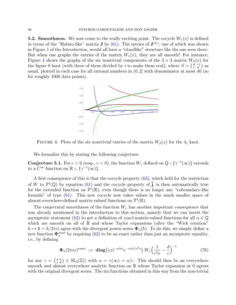
38 STAVROS GAROUFALIDIS AND DON ZAGIER
5.2. Smoothness. We now come to the really exciting point. The cocycle Wγ(x) is definedin terms of the “Habiro-like” matrix J by (61). The entries of J(41), one of which was shownin Figure 1 of the Introduction, would all have a “cloudlike” structure like the one seen there.But when one graphs the entries of the matrix Wγ(x), they are all smooth! For instance,Figure 4 shows the graphs of the six nontrivial components of the 3 × 3 matrix WS(x) forthe figure 8 knot (with three of them divided by i to make them real), where S =
(0 −11 0
)as
usual, plotted in each case for all rational numbers in (0, 2] with denominator at most 40 (sofor roughly 1000 data points).
0.2 0.4 0.6 0.8 1.0 1.2 1.4
-1.5
-1.0
-0.5
0.5
1.0
1.5
Figure 4. Plots of the six nontrivial entries of the matrix WS(x) for the 41 knot.
We formalize this by stating the following conjecture:
Conjecture 5.1. For c > 0 (resp., c < 0), the function Wγ defined on Qr{γ−1(∞)} extendsto a C∞ function on Rr {γ−1(∞)}.
A first consequence of this is that the cocycle property (63), which held for the restriction
of W to P1(Q) by equation (61) and the cocycle property of j, is then automatically truefor the extended function on P1(R), even though there is no longer any “coboundary-likeformula” of type (61). This new cocycle now takes values in the much smaller space ofalmost-everwhere-defined matrix-valued functions on P1(R).
The conjectural smoothness of the function Wγ has another important consequence thatwas already mentioned in the introduction to this section, namely that we can invert theasymptotic statement (62) to get a definition of exact matrix-valued functions for all α ∈ Qwhich are smooth on all of R and whose Taylor expansions (after the “Wick rotation”h 7→ ~ = h/2πi) agree with the divergent power series Φα(h). To do this, we simply define anew function Φexact
α by requiring (62) to be an exact rather than just an asymptotic equality,i.e., by defining
Φα(2πix)exact := diag(|cx|−κ(σ)e−v(σ)/c2x
)Wγ
( 1
c2x− d
c
)−1
(76)
for any γ =(a bc d
)∈ SL2(Z)) with α = γ(∞) = a/c. This should then be an everywhere
smooth and almost everywhere analytic function on R whose Taylor expansion at 0 agreeswith the original divergent series. The six functions obtained in this way from the non-trivial
KNOTS, PERTURBATIVE SERIES AND QUANTUM MODULARITY 39
elements of WS(x) for the figure 8 knot as plotted above (and multiplied by suitable powersof i to make them all real) are the ones shown in Figure 2 in the Introduction.
Apart from the numerical data, there are at least four reasons why we should expect thissmoothness property of the function Wγ to hold:
1. At the simplest level, equation (62) tells us that the matrix Wγ(X) is at least asymptot-ically smooth in the limit as X →∞ through rational numbers with bounded denominator,since it agrees to all orders in 1/X with a power series in 1/X with coefficients that do notdepend on the denominator or other arithmetic properties of X. Stated more visually, ifwe were to display the the components of Wγ(X) by plotting their values, for instance, forrational values of X between 1000 and 1001 and with denominators less than 100, then thesedata points would have to lie on a very smooth curve to very high precision.
2. In fact this same argument can be pushed much further, since by using the cocycleproperty (63) for x = X tending to infinity with bounded denominator we get a descriptionof the asymptotic behavior of Wg(x) in the neighborhood of any rational point, not merelyat infinity, and hence an explicit formula for its Taylor expansion at any rational point nearwhich it has a smooth expansion. This will be carried out in Proposition 5.2 below.
3. But the real reason that we expected the smoothness property is much deeper and alsopredicts (and in some cases leads to a proof of) much more: the entries of the matrix-valuedfunction Wγ(·) for a fixed γ extend to functions that are not merely smooth, but actuallyanalytic, on R r {−d/c}. This comes from the study of q-series associated to a knot andtheir relation to state integrals, as carried out in the companion paper [39] to this one, andwill be discussed in more detail in the final subsection of this section.
4. Finally, once one expects the real-analyticity, one can check it numerically using onlythe matrices studied in this paper, without any reference to either q-series or state integrals,by computing many Taylor coefficients of Wγ at any rational point using Proposition 5.2 andseeing that they now grow only polynomially rather than factorially. This point too will bediscussed in more detail in 5.4 below.
In the context just of this paper, where we are considering only functions on Q and formalpower series in h, but not holomorphic functions in the upper or lower half-planes or on cutplanes, we cannot justify the statement about analyticity or even continuity of the entriesof the matrix Wγ(·), i.e., we cannot show that the function Wγ(·) : Q r {−d/c} → C hasany natural extension to a matrix-valued function on Rr {−d/c}. However, as indicated inpoint 2. above, we can deduce a weaker statement if we assume the RQMC. To explain whatthis means, we must first discuss the various possible senses in which a function f : Q→ Ccan be continuous or differentiable. There are at least three different natural notions. Usuallyone considers the set of rational numbers with either the discrete topology or else the topologyinherited from their embedding into the reals. In the first sense, of course every fuctionfrom Q to C is continuous (i.e., f(α + εi) → f(α) for any sequence of rational numbersα + εi converging to α ∈ Q, since any such sequence is eventually constant) and in facteven C∞ (with the “Taylor expansion” of f at an arbitrary rational point α being justthe constant power series f(α)). In the second sense, one means that f(α + εi) → f(α)or f(α + εi) = Pα,d(εi) + o(εdi ) as i → ∞ for every α and every d ∈ N, where Pα,d is apolynomial of degree d and the εi are a sequence whose absolute values tend to 0 as i tends
40 STAVROS GAROUFALIDIS AND DON ZAGIER
to ∞. Such a function of course need not extend as a C∞ or even continuous function to R(an obvious counterexample being f(x) = 1/(x −
√2)), but if it does then this extension
is unique, so that the space C∞strong(Q) of smooth functions in this sense contains C∞(R) asa subspace. But there is a third sense, in which one requires f(α + εi) = f(α) + o(1) orf(α + εi) = Pα,d(εi) + o(εdi ) only for sequences {εi} of rational numbers that have boundednumerators but denominators tending to infinity (so that in particular they tend to 0 in theusual sense). We then have the strict inclusions
C∞(R) $ C∞strong(Q) $ C∞weak(Q) $ C∞discrete(Q) = CQ .
An example (courtesy of Peter Scholze) of a function f : Q → R that is C∞ in the weaksense but not in the srong sense is given by choosing a sequence of rational numbers {xn}tending to 0 and disjoint intervals In 3 xn with In containing no rational numbers withnumerator ≤ n; then define f to be 0 at x = 0 and to be the restriction of a C∞ functionon R∗ supported on ∪nIn and with f(xn) = 1, in which case f is obviously smooth in thestrong sense aways from 0 and in the weak sense at 0 (since the values of f on any sequenceof rational numbers tending to 0 with bounded numerators stabilizes to 0), but is not evencontinuous at 0.
After this lengthy preliminary discussion, we can state the result on the smoothnessproperties of the cocycle Wγ, with an explicit formula for the power series of Wγ(α+ ε) nearany α ∈ Q. We will write ε as −~ to match our previous conventions.
Proposition 5.2 (Assuming RQMC). The function Wγ belongs to C∞weak(Qr {γ−1(∞}) forevery γ ∈ PSL2(Z). Explicitly, Wγ(α− ~) for α 6= γ−1(∞) and ~ tending to 0 with boundeddenominator is given to all orders in ~ by the power series
Wγ(α− ~) ≈ Φγα(2πi~∗)−1 diag( ∣∣∣den(γα) ~∗
den(α) ~
∣∣∣κ(σ)
ev(σ)λγ(α))
Φα(2πi~) , (77)
with ~∗ = ~/(cα + d)(cα− c~ + d) if γ =(a bc d
).
Proof. By the definition of weak smoothness on Q, we have to show that Wγ(α + ε) forfixed γ ∈ SL2(Z) and α ∈ Q is given to all orders by a power series in ε depending onlyon α and γ as ε tends to 0 through rational numbers with bounded numerator. If we writeα as a′/c′ with a′ and c′ coprime and extend
(a′
c′
)to a matrix γ′ =
(a′ b′
c′ d′
)∈ SL2(Z), then the
condition of ε having bounded numerator is easily seen to be equivalent to the condition thatα+ ε = γ′X with X tending to ±∞ with bounded denominator. We consider first the casewhen X → +∞ (meaning that α+ ε tends to α from the left). By the cocycle property (63)and the basic asymptotic property (62) of Wγ we have
Wγ(α + ε) = Wγ(γ′X) = Wγγ′(X)Wγ′(X)−1
≈ Φa′′/c′′
( 2πi
c′′(c′′X + d′′)
)−1
Φa′/c′
( 2πi
c′(c′X + d′)
), (78)
where we have written γ =(a bc d
)and γγ′ = γ′′ =
(a′′ b′′
c′′ d′′
)and where ≈ as usual means that
the two expressions being compared are equal to all orders in 1/X as X tends to infinity
KNOTS, PERTURBATIVE SERIES AND QUANTUM MODULARITY 41
with bounded denominator or ε to zero with bounded numerator. If we now use our previousconventions, writing
−ε = ~ =1
c′(c′X + d′), ~∗ =
1
c′′(c′′X + d′′)=
c′2~c′′(c′′ − cc′~)
,
and also use that the “tweaking function” λγ satisfies
1
c′2~− 1
c′′2~∗=(X +
d′
c′
)−(X +
d′′
c′′
)=
c
c′c′′= λγ(α) , (79)
then we get equation (77) above. This equation expresses Wγ(α + ε) as a product of threematrices of power series in ~ = −ε and hence shows that it is itself such a matrix. This provesthe assertion in the first case X → +∞. To treat the case X → −∞ we use equation (72)instead of (62) and find that Wγ(α − ε) is given by the same formula as a product of threematrices of power series for ε > 0 as it was for ε < 0, because the prefactors B in (72) cancel.This completes the proof that Wγ is a two-sided smooth function on the rational numbersin the weak sense. �
Corollary 5.3. The function x 7→ Φα(2πix)exact on Q defined by (76) is differentiable inthe weak sense for every α ∈ Q.
Proof. This follows directly from Proposition 5.2 away from x = 0, since the diagonal pre-factor in (76) is smooth away from 0, and Φα(2πix)exact simply agrees with Φα(2πix) to allorders in x as x→ 0, so it is smooth there too. �
As a final remark in this subsection, we recall that in order to specify the cocycle γ 7→ Wγ
completely, it suffices to give its values for the two special matrices T =(
1 10 1
)and S =
(0 −11 0
),
since these generate the whole modular group. The function WT (x) is elementary (constantand conjugate to a diagonal matrix of Nth roots of unity, where N is the level of the knot).In the case where the level is 1, such as the 41 or 52 knots, WT is simply the identity matrixand the whole cocycle is determined by the single matrix-valued function WS(x). The factthat T 7→ 1, S 7→ WS extends to a cocycle on the whole group is then equivalent to therequirement that WS(x) satisfies the symmetry property
WS(x) = WS(−1/x)−1 , (80)
together with the three-term Lewis functional equation
WS(x) = WS(x+ 1)WS(x/(x+ 1)) , (81)
familiar from the theory of period polynomials of holomorphic modular forms on SL2(Z) orof period functions in the sense of [56] of Maass forms on SL2(Z). Our cocycles thus belongin some sense to the same family as periods of modular forms.
5.3. “Functions near Q”. We now come to an important and somewhat subtle point. Inthe calculation that we gave to prove Proposition 5.2, we used only the Refined QuantumModularity Conjecture in its “rational version” (57), since the statement of Proposition 5.2involves only the values of Wγ at rational arguments. If we had used instead the full ver-sion (58) of the RQMC, we would have obtained a stronger version of the “weakly smooth”condition that applies to approximating a rational number not just by rational numbers that
42 STAVROS GAROUFALIDIS AND DON ZAGIER
differ from it by a small rational number with bounded numerator, but also by infinitesimalvariations of such numbers. To make sense of a statement of this type, we now introducea notion that will shed more light on the two cocycles γ 7→ λγ and of γ 7→ Wγ and that isalso relevant in connection with the notion of “holomorphic quantum modular forms” thatwill be touched on briefly in Section 5.4 and developed in more detail in [39] and in thesurvey paper [71]. This is the notion of asymptotic functions near Q. The basic idea hereis to specify a particular type of asymptotic behavior (such as a formal power series) in aninfinitesimal neighborhood of every rational point, where “neighborhood” can mean that weapproach the rational number from the right and the left on the real line, or in other contextsfrom above and below in the upper and lower complex half-planes. Since there are manytypes of behavior that may be of interest, and since it is hard to give a general definitionthat includes all of the examples and all of the properties that one wishes to include, we willrestrict here to the particular classes that arise in the context of knot invariants.
The simplest version of this notion is just given by a collection {fα(ε)}α∈Q of formal powerseries with complex coefficients indexed by the rational numbers. Here we want to think ofthe infinitesimal power series variable ε as the difference between the rational number α andan infinitesimally nearby real “number” α + ε, i.e. we want to think of the whole collectionof power series {fα} as a single “asymptotic function near Q”, i.e., as a “function” f definedin infinitesimal neighborhoods of all rational points α by f(α+ε) = fα(ε). Of course f is nota function at all in the traditional sense, since one cannot evaluate it at numerical values ofits argument, but as we will see in a moment, this point of view is nevertheless very fruitful.It originally showed up in the paper [73], where “quantum modular forms” were first definedsimply as functions on Q (more precisely, as almost-everywhere-defined functions on Q) butthen upgraded to a notion of “strong quantum modular forms” where the original values atrational numbers became the constant terms of a collection of formal power series.
The set of asymptotic functions near Q (from now on we omit the quotation marks,trusting the reader to remember that these are not actually functions) of this special typeforms a ring via pointwise addition and multiplication if we think of its elements as collectionsof formal power series, and by straight addition and multiplication if we think of them asfunctions defined in infinitesimal neighbourhoods of all rational points. To understand itselements, it is helpful to think of the following two extreme cases.
(i) Each fα(ε) is the Taylor expansion∑f (n)(α) εn/n! of a function f ∈ C∞(R) at the
point α. Here the various asymptotic expansions near rational points fit togethernicely into a single smooth function on R.
(ii) Each fα(ε) is the formal power series expansion at q = e2πi(α+ε) of an element A(q)of the Habiro ring H = lim←−Z[q]/((q; q)n). Here the different power series do notin general fit together smoothly at all, and even their constant terms jump aroundwildly, as illustrated in Figure 1 in the introduction.
At first sight this definition seems to be pointless because we are not requiring any com-patibility at all between the different power series fα and therefore the ring we have justintroduced is canonically isomorphic the direct product C[[ε]]Q =
∏αC[[ε]] of one copy of the
power series ring C[[ε]] for every rational number α. The point, however, is that if we passto the quotient ring F0,0 ≈
∏αC[[ε]]/
⊕αC[[ε]] of asymptotic functions in the neighborhood
KNOTS, PERTURBATIVE SERIES AND QUANTUM MODULARITY 43
of all but a finite set of rational points, then the modular group Γ1 = SL2(Z) acts by sendingf to f ◦ γ for γ ∈ Γ1, and this action does not simply permute the different power series fαbut twists them as well. Specifically, if f(x) is represented near α by f(α + ε) = fα(ε)then f(γ(x)) is represented near α∗ = γ(α) by fα∗(ε
∗) rather than simply by fα∗(ε), whereε∗ = γ(α + ε) − γ(α), or more explicitly ε∗ = ε/(cα + d)(cα + d + cε) if γ =
(a bc d
). This
is precisely the twist that we already encountered in Section 3.2 (equations (29) and (32))and in Proposition 5.2 above, except that we have changed the previous variable h to −2πiεhere. (The rescaling of h by a factor 2πi was introduced for our knot invariants only to makethe power series coefficients algebraic and there is no reason to make this change of variablein the general situation.)
We now generalize the above notion by introducing two complex parameters v and κ andconsidering the vector space of asymptotic functions near Q whose local form fα(ε) = f(α+ε)in a real infinitesimal neighborhood of any α ∈ Q is given by
fα(ε) = |den(α) ε|κ e−v/den(α)2ε φα(ε) (82)
for some power series φα(v) ∈ C[[ε]]. Again we pass to the quotient Fκ,v of almost-everywhere-defined asymptotic functions on Q, i.e., we identify two collections of power series if they differfor only finitely many α. This space is a free module of rank 1 over the ring F0,0 introducedabove, and is again isomorphic to
∏αC[[ε]]/
⊕αC[[ε]] via f 7→ {φα}, but with a different
action of SL2(Z) than before. Specifically, γ ∈ SL2(Z) sends f to the function near Q thatcorresponds via (82) to the collection of power series {φ∗α(ε) = evλγ(α)φα∗(ε
∗)} with α∗ and ε∗
as above and with the “tweaking cocycle” λγ(α) introduced in (24). Alternatively, in termsof the variable x = α + ε infinitesimally near α ∈ Q we can write this action as the “slashaction” (familiar from the theory of modular forms if κ is an even integer, and from the theoryof the principal series representation of SL2(R) if not) given by (f |κγ)(x) = |cx+ d|−κf(γx)for γ =
(a bc d
)∈ SL2(Z), where |cx+d|−κ := |cα+d|−κ(1+ cε/(cα+d))−κ. This also explains
the reason for including the perhaps strange-looking factors den(α) and den(α)−2 in (82),since without them there would be no action of the modular group. We also point out that,because of the “tweaking” factor evλγ(α) in the definition of the action, Fκ,v is a free moduleof rank 1 over the ring F0,0 as a vector space, but not as an SL2(Z)-module: one cannotchoose a generator in an SL2(Z)-invariant way.
Of course from the point of view of this paper the main reason for introducing the param-eters κ and v and the definition (82) is that this is exactly the behavior that we found exper-imentally from the Refined Quantum Modularity Conjecture, with v = v(σ) and κ = κ(σ)being the normalized volume and weight associated to a parabolic flat connection σ and
with φa(ε) and fα(ε) being the power series Φ(K,σ)α (h) (or more generally Φ
(K,σ,σ′)α (h)) and
its completion Φ(K,σ)α (h) (or Φ
(K,σ,σ′)α (h)) as in (27), with h = −2πε. But it is worth noting
that the space Fκ,v also contains classical modular forms on the full modular group, since aholomorphic modular form f(τ) of (necessarily even) weight k on SL2(Z) defines a functionnear Q of type (82) with κ equal to −k, with v equal to −2πi times the valuation of fat infinity (the smallest exponent of q = e(τ) in the Fourier expansion of f(τ)), and witheach power series φα(ε) reducing to its constant term φα(0), as one sees easily by using themodular transformation property of f to compute the asymptotic development of f(α + ε)
44 STAVROS GAROUFALIDIS AND DON ZAGIER
for α ∈ Q and ε tending to 0 with positive real part. More generally, mock modular forms(whose definition we omit) also define elements of Fκ,v, where κ is again the negative of theweight, but in that case the power series φα(ε) are in general factorially divergent rather thanconstant. We do not elaborate on any of this since it is far from the theme of this paper,but it is nice to observe that classical modular and mock modular forms have properties incommon with the asymptotic functions occurring here.
There are two further points that we should mention in connection with the definition (82).One is that the absolute value appearing there is only appropriate for ε real, which is ouroriginal situation when we think of α+ε as being a deformation of the rational number α onthe real line or when we take ε = −1/c(cX+d) with X a rational number tending to infinityas in the RQMC. But when we consider functions near Q in the complex as well as in thereal domain, the absolute value sign would destroy holomorphy. If κ is an even integer, theproblem does not arise, since we can simply replace |ε|κ by εκ, which is holomorphic. If thisis not the case then if we consider only functions near rational points in the upper or lowerhalf-plane, we can still replace |ε|κ in the definition by εκ, which makes sense because ε hasa well-defined logarithm in either half-plane. (We will never encounter functions in Fκ,v forκ 6= 0 that are defined in a 360o complete complex neighborhood of α; our functions willeither be defined for nearby real points or for nearby non-real points, or sometimes in a cutplane Cr (−∞, 0] or Cr [0,∞), in which case we can extend |ε|κ holomorphically as εκ or(−ε)κ, respectively.) However, when κ is not an integer and we want to discuss the SL2(Z)action on Fκ,v, then we have to include some kind of multiplier system, as familiar from thetheory of modular forms of arbitrary weight.
The second minor comment is that one can further generalize F0,0 by introducing a level Nas well as the parameters κ and v. This generalization is necessary if we want to includemodular or mock modular forms of level N (say on Γ = Γ0(N) or Γ(N)) into our definition,but also for our knot invariants if the knot has a level > 1, as we found to be the casefor the (−2, 3, 7)-pretzel knot. Here the power series φα(ε) and their completions will haveperiod N rather than 1 with respect to α, and more importantly, the number v in (82) isno longer constant but must be replaced by a number vα that depends on the Γ-equivalenceclass (“cusp”) of α. Again we omit details, since this is not our main subject.
We now return to the functions studied in this paper and to the reason why we introducedasymptotic functions near Q in the first place. Consider first the tweaking function definedby equation (24). We showed in Lemma 3.1 that the map γ 7→ λγ is a cocycle in the space ofalmost-everywhere-defined functions on P1(Q). It is easily checked that it is not a coboundaryin that space. But if we extend λγ to a function near Q by setting λγ(α+ε) = λγ(α) (constantpower series), then equation (79) says that it now is a coboundary: λγ(x) = µ(x) − µ(γx)where µ is the function near Q defined by µ(α + ε) = 1/den(α)2ε . More interestingly, if
for each σ and σ′ in PK we define a function near Q by Q(K,σ,σ′)(α − ~) = Φ(K,σ,σ′)α (h) and
then put them together as a matrix-valued function Q near Q given by Q(α−~) = Φ(K)α (h),
then using equation (79) again we see that the complicated equation (77) becomes the muchsimpler equation
Wγ(x) = Q(γx)−1 Q(x) . (83)
KNOTS, PERTURBATIVE SERIES AND QUANTUM MODULARITY 45
Notice that in this equation the (σ, σ′)-entry on the left-hand side is the sum over σ′′ ∈ PKof the product of the (σ, σ′′)-entry of Q(γx)−1 and the (σ′′, σ′)-entry of Q(x), which belongto F−κ(σ′′),−v(σ′′) and Fκ(σ′′),v(σ′′), respectively. Thus each of the terms of the sum belongsto F0,0 and we never encounter the problem of having to make sense of sums of asymptoticfunctions of different orders of growth. The fact that the entries of Wγ all belong to F0,0 is,of course, a necessary prerequisite for the final statement that they actually belong to itssubring C∞(R).
Equation (83) tells us us the cocycle γ 7→ Wγ, which was not a coboundary in thespace of almost-everywhere-defined matrix-valued functions on P1(Q) or of piecewise smoothfunctions on P1(R), becomes one when we pass to the space of matrix-valued functionsnear Q. Both of these can be seen as manifestations of a general phenomenon that one findsin almost all mathematical contexts where notions of homology or cohomology play a role:even though one is really only interested in cocycles that are not coboundaries, the cocyclesthat one studies are almost always constructed as coboundaries in some bigger space.
5.4. Analyticity. In Subsection 5.2 we discussed the surprising smoothness properties ofthe function Wγ on Rr{γ−1(∞)}. In this subsection, we come to a point much deeper thanthe smoothness, namely analyticity properties of functions defined in a cut plane. Thesefunctions are closely related to state integrals. Such integrals appeared originally in the workof Hikami, Andersen, Kashaev and others (see for example [48, 15, 1]) in relation to thepartition function of complex Chern-Simons theory and to quantum Teichmuller theory, andreappear in our context in [39], the sequel paper to this one.
State integrals are analytic functions with several key features:
• They are holomorphic for all τ ∈ C′ = Cr (−∞, 0] .• Their restrictions to CrR factorize bilinearly as finite sums of products of a q-series
and a q-series, where q = e(τ) and q = e(−1/τ); see [3, 29].• Their evaluation at positive rational numbers also factorizes bilinearly as a finite sum
of a product of a periodic function of τ and a periodic function of −1/τ ; see [28].
They are defined as multidimensional integrals of a product of quantum dilogarithms timesthe exponential of a quadratic form. The quantum dilogarithm, invented by Faddeev [18,19], is a remarkable meromorphic function of two variables. The structure of its polesimplies that the state integrals are holomorphic functions of τ in the cut plane C′. Thequantum dilogarithm is also a quasi-periodic function with two quasi-periods, and this hastwo consequences, one of which is directly related to the third “feature” above, and the otherto the second “feature” and to the paper [39].
The first consequence is the fact that one can apply the residue theorem to give an exactformula for the values of the state-integrals at positive rational numbers. Such a formulawas given explicitly for the one-dimensional state integrals considered in Equation (1) andTheorem 1.1 of [28], and those one-dimensional state integrals cover the case of the threeknots that we consider here, namely the 41, 52 and (−2, 3, 7) pretzel knot. It turns out thatEquation (15) of [28] applied to the case of (A,B) = (1, 2) gives a function on Q+ which isnone other than one of our four entries of Wγ when γ = S. To get the other three entriesof WS, one can apply the proof of [28] to a 2 × 2 matrix of state-integrals of the 41 knot
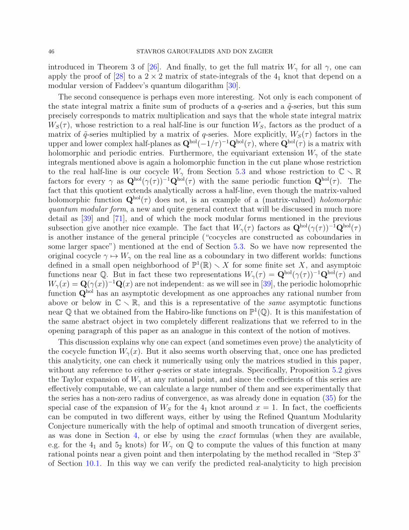
46 STAVROS GAROUFALIDIS AND DON ZAGIER
introduced in Theorem 3 of [26]. And finally, to get the full matrix Wγ for all γ, one canapply the proof of [28] to a 2 × 2 matrix of state-integrals of the 41 knot that depend on amodular version of Faddeev’s quantum dilogarithm [30].
The second consequence is perhaps even more interesting. Not only is each component ofthe state integral matrix a finite sum of products of a q-series and a q-series, but this sumprecisely corresponds to matrix multiplication and says that the whole state integral matrixWS(τ), whose restriction to a real half-line is our function WS, factors as the product of amatrix of q-series multiplied by a matrix of q-series. More explicitly, WS(τ) factors in theupper and lower complex half-planes as Qhol(−1/τ)−1Qhol(τ), where Qhol(τ) is a matrix withholomorphic and periodic entries. Furthermore, the equivariant extension Wγ of the stateintegrals mentioned above is again a holomorphic function in the cut plane whose restrictionto the real half-line is our cocycle Wγ from Section 5.3 and whose restriction to C r Rfactors for every γ as Qhol(γ(τ))−1Qhol(τ) with the same periodic function Qhol(τ). Thefact that this quotient extends analytically across a half-line, even though the matrix-valuedholomorphic function Qhol(τ) does not, is an example of a (matrix-valued) holomorphicquantum modular form, a new and quite general context that will be discussed in much moredetail as [39] and [71], and of which the mock modular forms mentioned in the previoussubsection give another nice example. The fact that Wγ(τ) factors as Qhol(γ(τ))−1Qhol(τ)is another instance of the general principle (“cocycles are constructed as coboundaries insome larger space”) mentioned at the end of Section 5.3. So we have now represented theoriginal cocycle γ 7→ Wγ on the real line as a coboundary in two different worlds: functionsdefined in a small open neighborhood of P1(R) r X for some finite set X, and asymptoicfunctions near Q. But in fact these two representations Wγ(τ) = Qhol(γ(τ))−1Qhol(τ) andWγ(x) = Q(γ(x))−1Q(x) are not independent: as we will see in [39], the periodic holomoprhicfunction Qhol has an asymptotic development as one approaches any rational number fromabove or below in C r R, and this is a representative of the same asymptotic functionsnear Q that we obtained from the Habiro-like functions on P1(Q). It is this manifestation ofthe same abstract object in two completely different realizations that we referred to in theopening paragraph of this paper as an analogue in this context of the notion of motives.
This discussion explains why one can expect (and sometimes even prove) the analyticity ofthe cocycle function Wγ(x). But it also seems worth observing that, once one has predictedthis analyticity, one can check it numerically using only the matrices studied in this paper,without any reference to either q-series or state integrals. Specifically, Proposition 5.2 givesthe Taylor expansion of Wγ at any rational point, and since the coefficients of this series areeffectively computable, we can calculate a large number of them and see experimentally thatthe series has a non-zero radius of convergence, as was already done in equation (35) for thespecial case of the expansion of WS for the 41 knot around x = 1. In fact, the coefficientscan be computed in two different ways, either by using the Refined Quantum ModularityConjecture numerically with the help of optimal and smooth truncation of divergent series,as was done in Section 4, or else by using the exact formulas (when they are available,e.g. for the 41 and 52 knots) for Wγ on Q to compute the values of this function at manyrational points near a given point and then interpolating by the method recalled in “Step 3”of Section 10.1. In this way we can verify the predicted real-analyticity to high precision
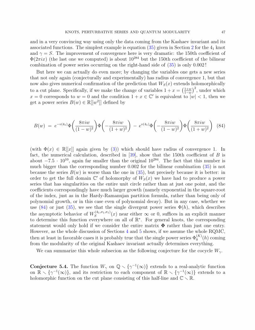
KNOTS, PERTURBATIVE SERIES AND QUANTUM MODULARITY 47
and in a very convincing way using only the data coming from the Kashaev invariant and itsassociated functions. The simplest example is equation (35) given in Section 2 for the 41 knotand γ = S. The improvement of convergence here is very dramatic: the 150th coefficient ofΦ(2πix) (the last one we computed) is about 10284 but the 150th coefficient of the bilinearcombination of power series occurring on the right-hand side of (35) is only 0.002 !
But here we can actually do even more; by changing the variables one gets a new seriesthat not only again (conjecturally and experimentally) has radius of convergence 1, but thatnow also gives numerical confirmation of the prediction that WS(x) extends holomorphically
to a cut plane. Specifically, if we make the change of variables 1 + x =(
1+w1−w
)2, under which
x = 0 corresponds to w = 0 and the condition 1 + x ∈ C′ is equivalent to |w| < 1, then weget a power series B(w) ∈ R[[w2]] defined by
B(w) = e−v(41)Φ
(8πiw
(1− w)2
)Φ
(− 8πiw
(1 + w)2
)− ev(41)Φ
(− 8πiw
(1− w)2
)Φ
(8πiw
(1 + w)2
)(84)
(with Φ(x) ∈ R[[x]] again given by (3)) which should have radius of convergence 1. Infact, the numerical calculation, described in [39], show that the 150th coefficient of B isabout −7.5 · 1010, again far smaller than the original 10284. The fact that this number ismuch bigger than the corresponding number 0.002 for the bilinear combination (35) is notbecause the series B(w) is worse than the one in (35), but precisely because it is better: inorder to get the full domain C′ of holomorphy of WS(x) we have had to produce a powerseries that has singularities on the entire unit circle rather than at just one point, and thecoefficients correspondingly have much larger growth (namely exponential in the square-rootof the index, just as in the Hardy-Ramanujan partition formula, rather than being only ofpolynomial growth, or in this case even of polynomial decay). But in any case, whether weuse (84) or just (35), we see that the single divergent power series Φ(h), which describes
the asymptotic behavior of W(41,σ1,σ1)S (x) near either ∞ or 0, suffices in an explicit manner
to determine this function everywhere on all of R∗. For general knots, the correspondingstatement would only hold if we consider the entire matrix Φ rather than just one entry.However, as the whole discussion of Sections 4 and 5 shows, if we assume the whole RQMC,
then at least in favorable cases it is probably true that the single power series Φ(K)0 (h) coming
from the modularity of the original Kashaev invariant actually determines everything.
We can summarize this whole subsecion as the following conjecture for the cocycle Wγ.
Conjecture 5.4. The function Wγ on Q r {γ−1(∞)} extends to a real-analytic functionon R r {γ−1(∞)}, and its restriction to each component of R r {γ−1(∞)} extends to aholomorphic function on the cut plane consisting of this half-line and Cr R.
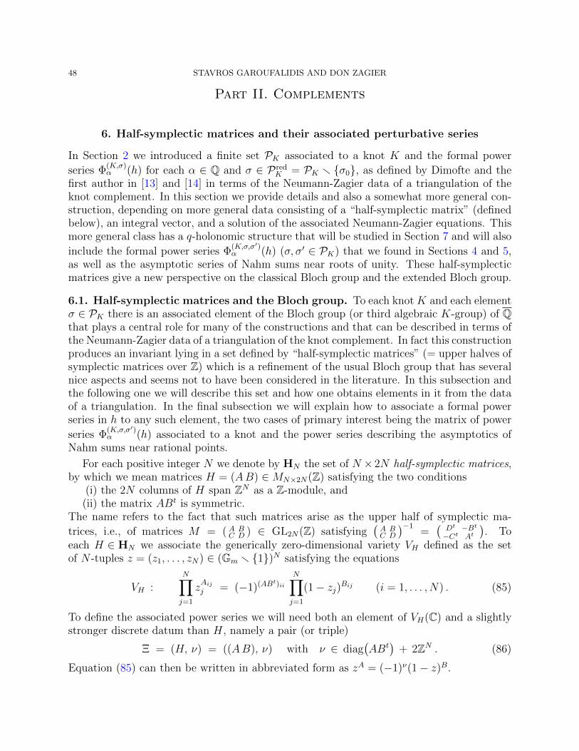
48 STAVROS GAROUFALIDIS AND DON ZAGIER
Part II. Complements
6. Half-symplectic matrices and their associated perturbative series
In Section 2 we introduced a finite set PK associated to a knot K and the formal power
series Φ(K,σ)α (h) for each α ∈ Q and σ ∈ Pred
K = PK r {σ0}, as defined by Dimofte and thefirst author in [13] and [14] in terms of the Neumann-Zagier data of a triangulation of theknot complement. In this section we provide details and also a somewhat more general con-struction, depending on more general data consisting of a “half-symplectic matrix” (definedbelow), an integral vector, and a solution of the associated Neumann-Zagier equations. Thismore general class has a q-holonomic structure that will be studied in Section 7 and will also
include the formal power series Φ(K,σ,σ′)α (h) (σ, σ′ ∈ PK) that we found in Sections 4 and 5,
as well as the asymptotic series of Nahm sums near roots of unity. These half-symplecticmatrices give a new perspective on the classical Bloch group and the extended Bloch group.
6.1. Half-symplectic matrices and the Bloch group. To each knot K and each elementσ ∈ PK there is an associated element of the Bloch group (or third algebraic K-group) of Qthat plays a central role for many of the constructions and that can be described in terms ofthe Neumann-Zagier data of a triangulation of the knot complement. In fact this constructionproduces an invariant lying in a set defined by “half-symplectic matrices” (= upper halves ofsymplectic matrices over Z) which is a refinement of the usual Bloch group that has severalnice aspects and seems not to have been considered in the literature. In this subsection andthe following one we will describe this set and how one obtains elements in it from the dataof a triangulation. In the final subsection we will explain how to associate a formal powerseries in h to any such element, the two cases of primary interest being the matrix of power
series Φ(K,σ,σ′)α (h) associated to a knot and the power series describing the asymptotics of
Nahm sums near rational points.
For each positive integer N we denote by HN the set of N × 2N half-symplectic matrices,by which we mean matrices H = (AB) ∈MN×2N(Z) satisfying the two conditions
(i) the 2N columns of H span ZN as a Z-module, and(ii) the matrix ABt is symmetric.
The name refers to the fact that such matrices arise as the upper half of symplectic ma-
trices, i.e., of matrices M = ( A BC D ) ∈ GL2N(Z) satisfying
(A BC D
)−1=(Dt −Bt−Ct At
). To
each H ∈ HN we associate the generically zero-dimensional variety VH defined as the setof N -tuples z = (z1, . . . , zN) ∈ (Gm r {1})N satisfying the equations
VH :N∏j=1
zAijj = (−1)(ABt)ii
N∏j=1
(1− zj)Bij (i = 1, . . . , N) . (85)
To define the associated power series we will need both an element of VH(C) and a slightlystronger discrete datum than H, namely a pair (or triple)
Ξ = (H, ν) = ((AB), ν) with ν ∈ diag(ABt
)+ 2ZN . (86)
Equation (85) can then be written in abbreviated form as zA = (−1)ν(1− z)B.
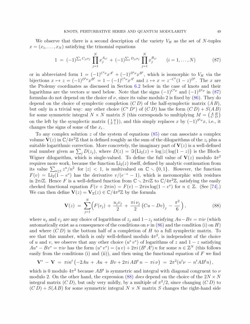
KNOTS, PERTURBATIVE SERIES AND QUANTUM MODULARITY 49
We observe that there is a second description of the variety VH as the set of N -tuplesx = (x1, . . . , xN) satisfying the trinomial equations
1 = (−1)∑j Cjiνj
N∏j=1
xAjij + (−1)
∑j Djiνj
N∏j=1
xBjij (i = 1, . . . , N) (87)
or in abbreviated form 1 = (−1)CtνxA
t+ (−1)D
tνxBt, which is isomorphic to VH via the
bijections x 7→ z = (−1)DtνxB
t= 1 − (−1)C
tνxAt
and z 7→ x = z−Ct(1 − z)D
t. The x are
the Ptolemy coordinates as discussed in Section 6.2 below in the case of knots and theirlogarithms are the vectors w used below. Note that the signs (−1)C
tν and (−1)Dtν in (87)
formulas do not depend on the choice of ν, since its value modulo 2 is fixed by (86). They dodepend on the choice of symplectic completion (C D) of the half-symplectic matrix (AB),but only in a trivial way: any other choice (C∗D∗) of (C D) has the form (C D) + S(AB)for some symmetric integral N ×N matrix S (this corresponds to multiplying M =
(A BC D
)on the left by the symplectic matrix
(1 0S 1
)), and this simply replaces x by (−1)S
tνx, i.e., itchanges the signs of some of the xi .
To any complex solution z of the system of equations (85) one can associate a complexvolume V(z) in C/4π2Z that is defined roughly as the sum of the dilogarithms of the zi plus asuitable logarithmic correction. More concretely, the imaginary part of V(z) is a well-definedreal number given as
∑j D(zj), where D(z) = =
(Li2(z) + log |z| log(1 − z)
)is the Bloch-
Wigner dilogarithm, which is single-valued. To define the full value of V(z) modulo 4π2
requires more work, because the function Li2(z) itself, defined by analytic continuation fromits value
∑n≥1 z
n/n2 for |z| < 1, is multivalued on C r {0, 1}. However, the function
F (v) = Li2(1 − ev) has the derivative v/(e−v − 1), which is meromorphic with residuesin 2πiZ. Hence F is a well-defined function from Cr 2πiZ to C/4π2Z, satisfying the easilychecked functional equation F (v + 2πin) = F (v) − 2πin log(1 − ev) for n ∈ Z. (See [74].)We can then define V(z) = VΞ(z) ∈ C/4π2Z by the formula
V(z) =N∑j=1
(F (vj) +
ujvj2
+πi νj
2
(Cu−Dv
)j− π2
6
), (88)
where uj and vj are any choice of logarithms of zj and 1−zj satisfying Au−Bv = πiν (whichautomatically exist as a consequence of the conditions on ν in (86) and the condition (i) onH)and where (C D) is the bottom half of a completion of H to a full symplectic matrix. Tosee that this number, which is only well-defined modulo 4π2, is independent of the choiceof u and v, we observe that any other choice (u∗ v∗) of logarithms of z and 1− z satisfyingAu∗ − Bv∗ = πiν has the form (u∗ v∗) = (u v) + 2πi (BtAt)n for some n ∈ ZN (this followseasily from the conditions (i) and (ii)), and then using the functional equation of F we find
V∗ − V = πint(−2Au + Au + Bv + 2πiABt n − πi ν
)= 2π2(ntν − ntABtn) ,
which is 0 modulo 4π2 because ABt is symmetric and integral with diagonal congruent to νmodulo 2. On the other hand, the expression (88) does depend on the choice of the 2N ×Nintegral matrix (C D), but only very mildly, by a multiple of π2/2, since changing (C D) to(C D) + S(AB) for some symmetric integral N × N matrix S changes the right-hand side
50 STAVROS GAROUFALIDIS AND DON ZAGIER
of (88) by −π2
2νtSν. We believe, but have not checked, that it should be possible to lift the
formula (88) to a formula giving VΞ(z) modulo 4π2 rather than just modulo π2/2 in termsof H alone by adding to the right-hand side a term rMπ
2/2 where e(rM/8) is the 8th rootof unity occurring in the transformation law of Siegel theta series with characteristics underthe action of the symplectic matrix M =
(A BC D
)as given by Igusa ([50], Theorem 3, p. 182).
We make two small remarks on the above formulas before proceeding. The first is thatthe term π
2νt(Cu − Dv) in (88) is needed, not only to make the expression on the right
independent of the choice of logarithms u and v modulo 4π2 (it is already independent ofthis choice modulo π2 even if this term is omitted), but in order to get the right imaginarypart: the imaginary part of F (v) is D(z) + =(uv)/2 for eu = 1 − ev = z, where D(z) isthe Bloch-Wigner dilogarithm as above, and it is only if we include the term with Cu−Dvin (88) that its imaginary part has the correct value
∑j D(zj). The other is that the vector
w := Dv − Cu whose scalar product with ν gave the correction term in (88) also gives aparametrization of the N × 2 matrix (u v) as (BtAt)w+ iπ(Dt, Ct)ν. (To see this, just writethe relationship of (u v) to ν and w as M ( u
−v ) = ( πiν−w ) and use the formula for M−1.) Thisis simply the logarithmic version of the alternative characterization of the variety VH givenin (87), with w = log x. Changing (u v) by 2πi(BtAt)n with n ∈ ZN corresponds to takinga different logarithm w of the same x.
We next turn to the relation between half-symplectic matrices and the Bloch group. Thelatter is an abelian group B(F ) which is defined for any field F of characteristic zero as thequotient of the kernel of the map d : Z[F ]→ Λ2(F×) sending [x] to x∧ (1−x) for x 6= 0, 1 bythe subgroup generated by the 5-term relation of the dilogarithm. But the precise definitionvaries slightly in the literature because of delicate 2- and 3-torsion issues arising from theparticular definition of the exterior square (for instance, does one require x∧ x = 0 for all xor just x ∧ y = −y ∧ x ?) and the particular choice of the 5-term relation, which potentiallycomes in 56 versions obtained from one another by replacing each of the 5 arguments by itsimages under the group generated by x 7→ 1/x and x 7→ 1 − x. In fact, we will need theextended Bloch group as introduced by Neumann [59] and studied further by Zickert andothers in [42, 76], but here also there are several versions. We recall the definition from [76]here, and then describe a small refinement and the relation to half-symplectic matrices.
Denote by C the set of pairs of complex numbers (u, v) with eu+ev = 1. This is an abeliancover of C×r {0, 1} via z = eu = 1− ev, with Galois group isomorphic to Z2. The extended
Bloch group B(C) as defined in [42] or [76] is the kernel of the map d : Z[C]→ Λ2(C), whereΛ2(C) is defined by requiring only x∧ y+ y∧x = 0 (rather than x∧x = 0, which is stronger
by 2-torsion) and where d maps [u, v] := [(u, v)] ∈ Z[C] to u ∧ v, divided by the lifted version
of the 5-term relation, namely, the Z-span of the set of elements∑5
j=1(−1)j[uj, vj] of Z(C)
satisfying (u2, u4) = (u1 +u3, u3 +u5) and (v1, v3, v5) = (u5 +v2, v2 +v4, u1 +v4). There is an
extended regulator map from B(C) to C/4π2Z given by mapping∑
[uj, vj] to∑L(uj, vj),
where L(u, v) = F (v) + 12uv − π2
6, which one can check vanishes modulo 4π2 on the lifted
5-term relation. One can also define B(F ) for any subfield F of C, such as an embedded
number field, by replacing C by the subset F consisting of pairs (u, v) with eu = 1− ev ∈ F .The relation of the Bloch group and the extended Bloch group to algebraic K-theory is
KNOTS, PERTURBATIVE SERIES AND QUANTUM MODULARITY 51
that B(F ) for any field F is isomorphic up to torsion to the algebraic K-group K3(F ) ([63]),with the Borel regulator map from K3(C) to C/π2Q being given at the level of the Blochgroup by dilogarithms, while the extended Bloch group of a number field F ⊂ C is isomorphicto K ind
3 (F ) ([76]), for which the Borel regulator lifts to C/4π2Z.
We extend this group slightly by replacing Z[C] by the larger group Z[C] ⊕ C and d by
a map from this group to Λ2(C)/(iπ ∧ iπ), still given on Z[C] by [u, v] 7→ u∧ v but now also
defined on C by d(x) = x ∧ (x + πi), which despite appearances is a linear map because of
the antisymmetry of ∧. We then divide the kernel of this new d by a larger set of relations,namely the same lifted 5-term relation as before (with C component equal to 0) togetherwith the relations ([u, v] + [v, u]− [u′, v′]− [v′, u′], 0) and ([u, v] + [−u, v − u+ πi], u) for all
(u, v) and (u′, v′) in C corresponding to the elements [z]+[1−z] and [z]+[1/z]. The extendedregulator map to C/4π2Z is now defined by mapping
(∑[uj, vj], x
)to∑L(uj, vj)− xπi/2,
which agrees with the previous definition when x is 0 and which can be checked to vanishalso on the new relations. The advantage of this further extension of the Bloch group is thatthe solutions (u, v) of the logarithmic Neumann-Zagier equations (i.e., the set of (u, v) ∈ C2N
with (uj, vj) ∈ C for each j and Au − Bv = πiν with ν as in (86)) now give an element of
B(C), namely the class ξ of the pair(∑N
j=1[uj, vj], w), where w = Cu−Dv as before. Using
the parametrization (u, v) = (BtAt)w+(CtDt)νiπ discussed above, we check easily that the
image of this in Λ2(C) under d is (νtCDtν) (iπ)∧(iπ), and its image under the regulator mapis precisely the number V(z) defined in (88). When (u, v) comes from a triangulation of a3-manifold, then the effect of the extended 5-term relation is precisely that of a (2,3)-Pachnermove (changing one triangulation to another by replacing two tetrahedra with a common
face by three tetrahedra with the same set of vertices), so that the element ξ ∈ B(C) is atopological invariant of the manifold.
We end this subsection by explaining briefly how half-symplectic matrices actually give anew description of the extended Bloch group as a quotient of Sp∞ by suitable relations. Herefor convenience we are writing SpN rather than Sp2N for the group of symplectic matricesof size 2N × 2N over Z, and Sp∞ for the projective limit of these groups with respect tothe natural inclusions SpN ↪→ SpN+1. It also turns out to be more convenient to defineSpN as the space of matrices M satisfyng HJ∗NH
t = J∗N instead of HJNHt = JN used
above, where JN =(
0 −1N1N 0
)and J∗N is the block diagonal matrix with N copies of J1 on
the diagonal, in which case the inclusion just sends M to M+ =(M 00 12
), and similarly the
lifted 5-term relations become much simpler with this convention. The relations that wedivide by are roughly as follows. The first is stability (identify [M ] and [M+]). Anotheris that we identify [M ] and
[(1 0S 1
)M]
with S integral and symmetric are equivalent. (Thiscorresponds to working with half-symplectic rather than full symplectic matrices.) A third
is that we identify M ∈ SpN with( g 0
0 gt−1
)M for any g ∈ GLN(Z). (This corresponds to
permuting the N relations (85) or multiplying one of them by a monomial in the others.) Afourth is to identify M with M
(P 00 P
)for any N ×N permutation matrix P , corresonding in
the geometric case to changing the numbering of the N simplices, and yet another (whichmaybe can be omitted) corresponds to relabelling the edges so that the shape parameterz goes to z′ or z′′. The main one, of course, is a symplectic-matrix version of the 5-term
52 STAVROS GAROUFALIDIS AND DON ZAGIER
relation. This was first discovered in the special case corresponding to the Nahm sums (89)by Sander Zwegers in an unpublished 2011 conference talk and then given in various versionsfor abritrary symplectic matrices by Dimofte and the first author in [13] and in unpublishedwork by Campbell Wheeler and Michael Ontiveros (MPIM). The set of equivalence classesbecomes an abelian group by setting [M ] + [M ′] equal to the class of
(M 00 M ′
)and −[M ] to
the class of M−1. To get a map from this group to the extended Bloch group of C, we haveto first enlarge it by looking at equivalence classes, not just of half-symplectic matrices H(which is enough by the second of the above equivalence relations above), but of pairsconsisting of a half-symplectic matrix H = (AB) together with a solution (u, v) ∈ C2N ofthe logarithmic NZ equations Au−Bv = πν with ν as in (86), with corresponding lifts of the5-term and of the various other relations. The map from this larger group to the extendedBloch group is then the one described in the previous paragraph. It is injective becausethe 5-terms relations defining the extended Bloch group all lift to corresponding relations atthe (half-) symplectic level. It is also surjective, as one can show using elements of the setSpN,N ′ = {M ∈ MN×N ′(Z) | MJ2NM
t = J2N ′} of “non-square symplectic matrices” (notethat this set is just SpN if N = N ′ and reduces to 0 if N ′ > N) together with the obviouscomposition maps SpN,N ′ × SpN ′,N ′′ → SpN,N ′′ , in order to eliminate superfluous relations.
(Roughly speaking, if∑N
j=1[uj, vj] is the Z[C]-component of an element of B(C) as definedabove, then we define N ′ ≤ N as the rank of the group generated by all uj and vj andobtain an element of SpN,N ′ by writing the u’s and v’s in terms of these generators, whichthen always satisfy a collection of NZ equations.) A more detailed discussion of this andof the whole relationship between half-symplectic matrices and Bloch groups, including ourversions of the 5-term relation lifted to symplectic and half-symplectic matrices, will be givenin a subsequent version of this preprint.
This concludes our discussion of jalf-symplectic matrices and the equations (85). Theseobjects arise in (at least) two different contexts, in 3-dimensional topology and in the studyof special q-hypergeometric series (Nahm sums). The former is of course the one that is ofmost relevance for this paper, and will be discussed in more detail in the next subsection,but after that we will also say something about Nahm sums because they will play a rolein the sequel [39] to this paper and also because they give the most elementary approach todefining the associated formal power series that are our main subject of interest.
6.2. Ideal triangulations and the Neumann-Zagier equations. In 3-dimensional ge-ometry, the shape of an ideal tetrahedron in H3 is encoded by a complex number z ∈ C r{0, 1}, the tetrahedron being the convex hull of the four points 0, 1,∞, z ∈ P1(C) = ∂(H3).An ideal triangulation of a 3-manifold with torus boundary components give rise to an equa-tion (85), where the variables zi solving the equations (85) are the shape parameters of thetetrahedra and the equations are the “gluing conditions” relating the shape parameters of thetetrahedra incident on the various edges of the triangulation and on the cusp. These gluingequations originated in the work of Thurston [64] and further studied in [60], where the keysymplectic property of the matrices (AB) was found. We explain very briefly how this worksfor 3-manifolds whose boundary component is a torus, equipped with an ideal triangulationwith N tetrahedra. Each edge of the triangulation gives rise to a gluing equation assertingthat the product of the shape parameters of all tetrahedra incident to that edge equals to 1.
KNOTS, PERTURBATIVE SERIES AND QUANTUM MODULARITY 53
The product of the gluing equations corresponding to all edges is identically 1, hence onegluing equation is redundant, and can be removed and replaced by the gluing equation of anontrivial peripheral curve. Since there are N edges, this gives a collection of N gluing equa-tions. If one is interested in the geometric solution that describes the complete hyperbolicstructure, where all the shape parameters have positive imaginary part, the above gluingequations are replaced by their stronger logarithmic form, where the right hand side is now2πi for each edge and 0 for the peripheral curve. Using the fact that the three shape param-eters z, z′ = 1/(1− z) and z′′ = 1− 1/z satisfy the relation zz′z′′ = −1, and in logarithmicform log z + log z′ + log z′′ = πi, it follows that we can eliminate one of the three variablesat each tetrahedron (after choosing a pair of opposite edges for each tetrahedron). Doingso, the logarithmic form of the gluing equations now become linear equations for log zi andlog(1−zi), whose coefficients give rise to the Neumann–Zagier matrices A and B, and whereright hand side is a distinguished flattening ν satisfying (86). The latter can presumablybe deduced from the “parity condition” for ideal triangulations proved by Neumann [58],but we have not checked this. Neumann–Zagier’s theorem is that the above matrix (A |B)is the upper half of a symplectic matrix with integer entries. Note that the correspondingpairs (H, z) and (Ξ, z) are called “NZ datum” and “enhanced NZ datum” in [13]. Note alsothat a different choice of opposite edges in each tetrahedron cyclically permutes the triple(zj, z
′j, z′′j ) and changes the corresponding Neumann–Zagier matrices, but does not change
the corresponding element of B(C).
The connection between gluing equations and symplectic matrices involves not only theshapes of ideal tetrahedra, but also their Ptolemy variables. The latter is an assignment ofnonzero complex numbers xi at each edge of an ideal triangulation that satisfy the Ptolemyequations, namely at each tetrahedron we have a quadratic equation x1x2±x3x4±x5x6 = 0(with suitable signs). The signs require either ordered triangulations or a choice of a Ptolemycocycle and a detailed description is given in [37, Eqn. 12.2] and also in [24, Sec.3]. In thecase of a knot complement, these xj are exactly the ones introduced in (87) (and related tow = Du − Cv by xj = ewj), which here becomes a system of quadratic trinomial relationsafter rescaling because in each of the column of the gluing equation matrices there are atmost 6 non-zero entries, corresponding to the six edges of the tetrahedron corresponding tothat column.
We mention in passing that the variety defined by just the first N−1 edge gluing equationsis 1-dimensional and that this curve is described by the vanishing of the A-polynomial A(`,m)(where ` is the longitude) as introduced subsequently in [10], and that the variety obtainedby adding taking the first N − 1 relations together with the relation mp`q = 1 for coprimeintegers p and q corresponds to the compact 3-manifold obtained by doing a (p, q) Dehnsurgery on the knot complement. A detailed discussion of the choices involved to write downthese matrices can be found in Section 2 and Appendix A of [13]. All of this data is standardin knot theory, and is computed explicitly for any given knot complement (or more generally,an ideal triangulation of a cusped hyperbolic 3-manifold) by the computer implementationof SnapPy [11].
Once an ideal triangulation ∆ of a 3-manifold M as above has been fixed, a solution zof its gluing equations gives rise via a developing map to a representation ρz (i.e., a group
54 STAVROS GAROUFALIDIS AND DON ZAGIER
homomorphism) of π1(M) in PSL2(C), well-defined up to conjugation. If we choose theNeumann-Zagier equations as above, the representation ρz is boundary-parabolic and givesrise to an element of the extended Bloch group [75] and has a well-defined complex volume;see [59] and also [37]. Thus, if ∆ is an ideal triangulation of a the complement of a knot K,we have a map z 7→ ρz from VH(C) to PK , and the complex volume of ρz ∈ PK coincideswith the the complex volume of z, as follows from the work of Neumann [59] and Zickert [76]on the extended Bloch group.
There are, however, several subtleties of the above construction which we should point out.For instance, there exist triangulations of hyperbolic knots for which the map VH(C)→ PKis not onto or even for which the complex solutions set VH(C) is empty (this can happeneven for triangulations of the complement of the 41 knot). In this paper, we will ignore theseissues and assume that we are dealing with ideal triangulations for which the map is onto.We will further restrict our attentions to knots for which the set PK is finite. (There areknown to be knots for which the variety PK has strictly positive dimension, but they aretoo complicated for the calculations in this paper to be carried out. We believe that in suchcases the right indexing set of our formal power series would be the set of components of PKor of VH(C).)
An alternative approach to the definition of the set PK comes from the branches of the A-polynomial curve above the point M = 1, where M is the eigenvalue of the meridian. Even ifthe SL2(C) character variety of decorated representations of a knot complement has positive-dimensional components, its image in C∗×C∗, as given by the eigenvalue of the meridian andthe longitude, is one-dimensonal, and (ignoring any zero-dimensional components) is definedby the zeros of the A-polynomial of the knot. The A-polynomial is discussed in detail in theappendix of [7]. We will focus on knots that satisfy the property that the number of parabolicrepresentations σ coincides with the degree of the A-polynomial of a knot with respect to thelongitude. Note that the Galois group Gal(Q/Q) acts on the set PK of boundary parabolicrepresentations. What’s more, in a boundary parabolic representation, the longitude haseigenvalue ±1 and this partitions the set PK into two subsets P±K , each of which is stableunder the action of Gal(Q/Q). The geometric representation lies in P−K ; see [8, Lem.2.2].
6.3. Nahm sums and the perturbative definition of the Φ-series. In this final subsec-tion we describe how to attach to Ξ = ((AB), ν) as in (86), a solution z of the equation (85)
and a number α ∈ Q a completed formal power series belonging to eV(z)/den(α)2hC[[h]]. Asalready stated in Section 2, this was done in [13] (for α = 0) and [14] (for general α) in thecontext of knot complements and Neumann-Zagier data. However, there is a completely dif-ferent situation where the same formal power series are attached to the same data (Ξ, z, α),namely the asymptotics near roots of unity of special q-hypergeometric series called Nahmsums. Since these are a little more elementary we will use them to explain the derivation ofthe formal power series.
We begin by recalling what Nahm sums are. The simplest one is defined by
FA,b(q) =∑
n1,...,nN≥0
q12ntAn+btn
(q; q)n1 · · · (q; q)nN∈ Z[[q]] , (89)
KNOTS, PERTURBATIVE SERIES AND QUANTUM MODULARITY 55
where A is a an even positive definite symmetric matrix in MN(Z) and b an element of ZN .Changing each nj by 1, we see that the stationary points of the summand (i.e. the placeswhere nearby terms are asymptotically equal, giving the expected main contributions tothe whole sum) are given in the limit q → 1 by qnj = zj + o(1), where z = (z1, . . . , zN)is a solution of Nahm’s equation 1 − z = zA (which is the special case B = 1N of (85),with (A1N) being half-symplectic). Nahm observed that for any solution z of this equationthe element
∑i[zi] belongs to the Bloch group B(C) and conjectured that FA,b(q) (up to a
rational power of q, and considered as a function of τ with q = e(τ)) can only be a modularfunction if at least one solution of the Nahm equation has a trivial class in the Bloch group,and conversely that FA,b (again up to a power of q and as a function of τ) is a modularfunction of τ for some b if all solutions of the Nahm equation have trivial class in the Blochgroup. The first assertion was proved in [9]; the second is still open.
If we now generalize the Nahm sum to
FΞ(q) =∑
n∈ZN , Btn≥0
(−1)νtn q
12
(ntABtn+νtn)
(q; q)(Btn)1 · · · (q; q)(Btn)N
=∑
m,n∈ZN≥0×ZN
m=Btn
(−1)νtn q
12
(ntAm+νtn)
(q; q)m1 · · · (q; q)mN, (90)
with Ξ = ((AB), ν) as in (86), which is still a power series in q because of the congruencecondition on ν, then the same consideration as before shows that the stationary points of thesum correspond via z = qB
tn to the solutions of the equation (85). A formal computation ofthe contribution of the summands near these stationary point will lead to the perturbativeseries in h that we are looking for, where q = e−h with h→ 0, and in some cases one can showthat these h-series actually do describe the radial asymptotics of the Nahm sum (see [41],where this is shown to be the case for the original Nahm sum (89) and the real solution ofthe Nahm equation), but in general the calculation is purely formal because unless all zi arebetween 0 and 1 the series corresponding to h will not correspond to any subsum of (89)or (90). We also mention that there are even more general Nahm sums whose n-th summand(n ∈ ZN) is the product of a root of unity, a power of q given by a quadratic function of n,and a product of Pochhammer symbols (possibly to integer powers) with linear forms in nas arguments, which occur in several places in quantum topology, e.g. the 3D-index [12] andmany of the q-series in [39].
We now explain how to associate to the datum Ξ = (H, ν) and point z on VH a formal
power series Φ(Ξ,z)α (h) for each α ∈ Q/Z. We will do this first for the easier case α = 0, and
then discuss how the formula changes in the general case. The calculations for α = 0 weredone first for the simplest Nahm sum (89) in [72] and [67] and for general half-symplecticmatrices (AB) (though under the assumption that B is invertible over Q) in the contextof knots in [13]. The power series that were obtained in these two different contexts weresyntactially identical, and this coincidence persisted for general α, with the perturbativeseries of [14] being syntactically equal to the asymptotics of Nahm sums at roots of unity [41,Sec.5], with the formulas in all cases being given in terms of (sums of) formal Gaussianintegrals. It is for this reason that we can use the easier Nahm sums to motivate the preciseform of the integral to be studied. We only sketch the argument, referring to the papersabove for more details.
56 STAVROS GAROUFALIDIS AND DON ZAGIER
We begin by rewriting the first definition in (90) in the form
F(AB),ν(q) =1
(q; q)N∞
∑n∈ZN
(−1)νtn q
12
(ntABtn+νtn)
N∏j=1
(q(Btn)j+1; q
)∞ , (91)
where we no longer have to restrict to n with Btn ≥ 0 because (qm+1; q)∞ vanishes form ∈ Z<0. We must assume for now that the symmetric matrix ABt is positive definite toensure the convergence of the series (90) or (91), but this is not important at the end sincethe final formulas will be purely algebraic and make sense without this assumption. The keypoint is that if q = e−h with h small then the sum will be approximated to all orders bythe corresponding integral, with ZN replaced by RN and the summation sign by an integralsign. (This is a consequence of the Poisson summation formula, which represents the sumover ZN of a sufficiently smooth function of sufficiently rapid decay as the sum over ZN ofits Fourier coefficient, whose constant term is the integral corresponding to the original sumand whose other terms are of smaller order.) We then look at the expansion of the integrandaround its stationary points and approximate each by a Gaussian times a power series ina small local variable, as is always done in perturbation theory. The stationary points areindexed by the complex points z of VH , as already indicated, the correspondence being givenby q(Btn)j ∼ zj. On the other hand, for z ∈ C∗, q = e−h with h tending to 0, and t eitherfixed or growing more slowly than any power of 1/h, we have the asymptotic formula
1
(zet√h; q)∞
∼ exp
( ∞∑m=0
Bm
(t/√h)
m!Li2−m(z)hm−1
)(92)
= exp
(Li2(z)
h+( t√
h− 1
2
)log( 1
1− z
)+t2
2
z
1− z+ (small)
),
where Bm(t) denotes the m-th Bernoulli polynomial and “(small)” is an explicit power series
in t and√h with no constant term in
√h. (The first statement is [72, Lemma, p. 53] and the
second follows because all contributions from Bm(t/√h) with m ≥ 2 except for the quadratic
part of the B2-term are small.) Inserting this into the parts near the stationary points ofthe integral corresponding to the sum (91), we find after some calculation that the tot41alcontribution of the stationary part corresponding to a given solution z of (85) is eV(z)/h times
an explicit power series in h (initially in√h, but then in h because of the parity properties
of Bernoulli polynomials) which is written out in [13]. We only mention here that the powerseries obtained has coefficients in Q(z) (and hence in Fσ in our application to knots) exceptfor a prefactor det(A+B diag(zj/(1−zj))−1/2 coming from the determinant of the quadraticpart of the Gaussian.
When α = a/c is not integral, the calculations, done in [14] in the general case (still withB invertible) and in [41] for the special Nahm sums (89), are much more complicated andwe refer to those papers for the explicit formulas. A key point is that the stationary pointsof the integral are now indexed by the c-th roots of the solutions z of (85), but with thequadratic form appearing in the Gaussian depending only on z and not on the choice of c-th
root. This means that each of the formal power series Φ(Ξ,z)α (h) has the form of a sum over
(Z/cZ)N (after choosing some fixed c√z) of expressions similar to those occurring for the
KNOTS, PERTURBATIVE SERIES AND QUANTUM MODULARITY 57
simpler case c = 1. The reader can get a feeling for the nature of the formulas appearingby looking at Section 8 of this paper, where they are carried out in detail for the Kashaevinvariant of the 41 knot, this case however being deceptively simple because of the positivityof all of the terms occurring.
We make one final remark. The specific formulas given in [13] and [14] gave only the
series Φ(K,σ)α as discussed in Section 2, i.e., only the first column of our matrix Φ(K), because
the vector ν was always assumed to be the one coming from the geometric “flattening.” Byvarying ν, one can get the other columns of Φ. This variation produces a q-holonomic systemthat turns out to be closely related to the ones for the generalized Kashaev invariants thatwere discussed in 7.1. This will be the theme of the next section.
7. Two q-holonomic modules
In Part I we were led by the Refined Quantum Modularity Conjecture to find an entirematrix J(K) of Habiro-like functions generalizing the Kashaev invariant, the first columnbeing the vector of formal power series found in [13] and [14]. In this section we will studythe structure of the other columns of this matrix and will see that they have a natural “q-holonomic structure” in terms of an infinite collection of functions that satisfy a recursionof finite length and hence all lie in a finite-dimensional module. In section 7.1 we explainthis in detail for the case of the 41 knot, where explicit formulas for the entries of J(K)
were already given in Part I. In the next subsection we give the corresponding formulas,where the matrix in question has size 4 × 4 instead of 3 × 3. These are considerably morecomplicated for the 52 knot and have the interesting new feature that Dedekind sums appear.In subsection 7.3 we explain how these formulas could be guessed. This Ansatz involvesstudying the q-hypergeometric series defining the original Kashaev invariant via stationarypoints and formal Gaussian summation, analogous to what was done in Section 6.3 for Nahmsums and what will be done in Section 8 for the Kashaev invariant of the 41 knot. In thefinal subsection we discuss the point already alluded to at the end of Section 6 that thepower series in h studied there have a q-holonomic structure with the same coefficients asthe one associated to the matrix J. This is for the momenta purely experimental and is oneof the many mysteries associated with the subject. In Subsection 7.4 we also briefly mentiontwo further conjectural objects associated to knots (or more generally to half-symplecticmatrices) that we believe share the same q-holonomic structure.
7.1. Descendant Habiro-like functions. It turns out that the first row of J and the firstrow of Φ are basis elements of the span of an inhomogeneous recursion, and the same holds(but now with the corresponding homogeneous recursion) for each of the remaining rows of J
and of Φ as well as for the matrix of q-series of the forthcoming paper [39]. To illustrate howthis works, we give the complete formulas for the matrix for the 41 knot. The correspondingformulas for the 52 knot, which are considerably more complicated and illustrate severalfurther refinements (like the appearance of Dedekind sums), will be given in Section 7.3.
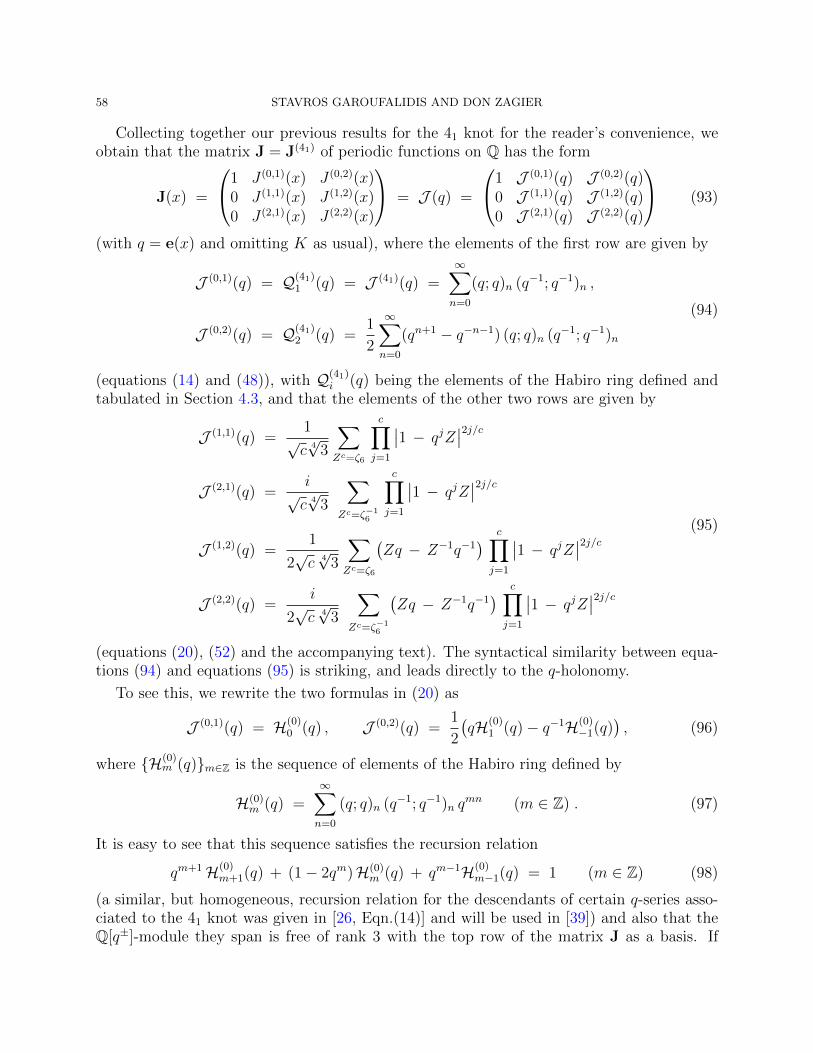
58 STAVROS GAROUFALIDIS AND DON ZAGIER
Collecting together our previous results for the 41 knot for the reader’s convenience, weobtain that the matrix J = J(41) of periodic functions on Q has the form
J(x) =
1 J (0,1)(x) J (0,2)(x)0 J (1,1)(x) J (1,2)(x)0 J (2,1)(x) J (2,2)(x)
= J (q) =
1 J (0,1)(q) J (0,2)(q)0 J (1,1)(q) J (1,2)(q)0 J (2,1)(q) J (2,2)(q)
(93)
(with q = e(x) and omitting K as usual), where the elements of the first row are given by
J (0,1)(q) = Q(41)1 (q) = J (41)(q) =
∞∑n=0
(q; q)n (q−1; q−1)n ,
J (0,2)(q) = Q(41)2 (q) =
1
2
∞∑n=0
(qn+1 − q−n−1) (q; q)n (q−1; q−1)n
(94)
(equations (14) and (48)), with Q(41)i (q) being the elements of the Habiro ring defined and
tabulated in Section 4.3, and that the elements of the other two rows are given by
J (1,1)(q) =1
√c 4√
3
∑Zc=ζ6
c∏j=1
∣∣1 − qjZ∣∣2j/c
J (2,1)(q) =i
√c 4√
3
∑Zc=ζ−1
6
c∏j=1
∣∣1 − qjZ∣∣2j/c
J (1,2)(q) =1
2√c 4√
3
∑Zc=ζ6
(Zq − Z−1q−1
) c∏j=1
∣∣1 − qjZ∣∣2j/c
J (2,2)(q) =i
2√c 4√
3
∑Zc=ζ−1
6
(Zq − Z−1q−1
) c∏j=1
∣∣1 − qjZ∣∣2j/c
(95)
(equations (20), (52) and the accompanying text). The syntactical similarity between equa-tions (94) and equations (95) is striking, and leads directly to the q-holonomy.
To see this, we rewrite the two formulas in (20) as
J (0,1)(q) = H(0)0 (q) , J (0,2)(q) =
1
2
(qH(0)
1 (q)− q−1H(0)−1(q)
), (96)
where {H(0)m (q)}m∈Z is the sequence of elements of the Habiro ring defined by
H(0)m (q) =
∞∑n=0
(q; q)n (q−1; q−1)n qmn (m ∈ Z) . (97)
It is easy to see that this sequence satisfies the recursion relation
qm+1H(0)m+1(q) + (1− 2qm)H(0)
m (q) + qm−1H(0)m−1(q) = 1 (m ∈ Z) (98)
(a similar, but homogeneous, recursion relation for the descendants of certain q-series asso-ciated to the 41 knot was given in [26, Eqn.(14)] and will be used in [39]) and also that theQ[q±]-module they span is free of rank 3 with the top row of the matrix J as a basis. If
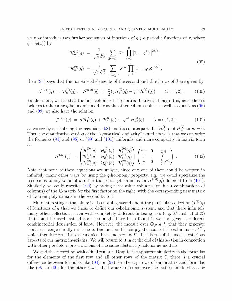
KNOTS, PERTURBATIVE SERIES AND QUANTUM MODULARITY 59
we now introduce two further sequences of functions of q (or periodic functions of x, whereq = e(x)) by
H(1)m (q) =
1√c 4√
3
∑Zc=ζ6
Zm
c∏j=1
∣∣1 − qjZ∣∣2j/c ,
H(2)m (q) =
i√c 4√
3
∑Zc=ζ−1
6
Zm
c∏j=1
∣∣1 − qjZ∣∣2j/c , (99)
then (95) says that the non-trivial elements of the second and third rows of J are given by
J (i,1)(q) = H(i)0 (q) , J (i,2)(q) =
1
2
(qH(i)
1 (q)− q−1H(i)−1(q)
)(i = 1, 2) . (100)
Furthermore, we see that the first column of the matrix J, trivial though it is, neverthelessbelongs to the same q-holonomic module as the other columns, since as well as equations (96)and (99) we also have the relation
J (i,0)(q) = qH(i)1 (q) + H(i)
0 (q) + q−1H(i)−1(q) (i = 0, 1, 2) , (101)
as we see by specializing the recursion (98) and its counterparts for H(1)m and H(2)
m to m = 0.Then the quantitative version of the “syntactical similarity” noted above is that we can writethe formulas (94) and (95) or (99) and (101) uniformly and more compactly in matrix formas
J (41)(q) =
H(0)−1(q) H(0)
0 (q) H(0)1 (q)
H(1)−1(q) H(1)
0 (q) H(1)1 (q)
H(2)−1(q) H(2)
0 (q) H(2)1 (q)
q−1 0 1
2q
1 1 0q 0 −1
2q−1
. (102)
Note that none of these equations are unique, since any one of them could be written ininfinitely many other ways by using the q-holonomy property, e.g., we could specialize therecursions to any value of m other than 0 to get formulas for J (i,0)(q) different from (101).Similarly, we could rewrite (102) by taking three other columns (or linear combinations ofcolumns) of the H-matrix for the first factor on the right, with the corresponding new matrixof Laurent polynomials in the second factor.
More interesting is that there is also nothing sacred about the particular collection H(i)(q)of functions of q that we chose to define our q-holonomic system, and that there infinitelymany other collections, even with completely different indexing sets (e.g. Z2 instead of Z)that could be used instead and that might have been found it we had given a differentcombinatorial description of knot. However, the module over Q[q, q−1] that they generateis at least conjecturally intrinsic to the knot and is simply the span of the columns of J(K),which therefore constitute a canonical basis indexed by P . This is one of the most mysteriousaspects of our matrix invariants. We will return to it in at the end of this section in connectionwith other possible representations of the same abstract q-holonomic module.
We end the subsection with a final remark. Despite the apparent similarity in the formulasfor the elements of the first row and all other rows of the matrix J, there is a crucialdifference between formulas like (94) or (97) for the top rows of our matrix and formulaslike (95) or (99) for the other rows: the former are sums over the lattice points of a cone
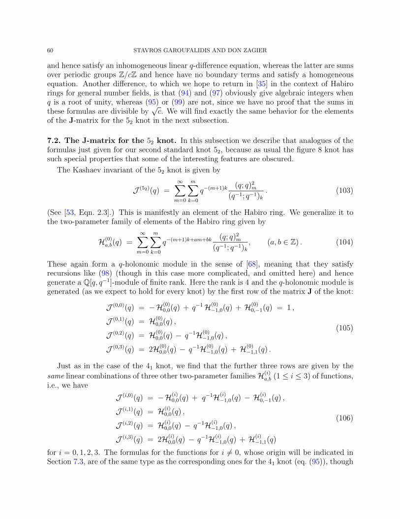
60 STAVROS GAROUFALIDIS AND DON ZAGIER
and hence satisfy an inhomogeneous linear q-difference equation, whereas the latter are sumsover periodic groups Z/cZ and hence have no boundary terms and satisfy a homogeneousequation. Another difference, to which we hope to return in [35] in the context of Habirorings for general number fields, is that (94) and (97) obviously give algebraic integers whenq is a root of unity, whereas (95) or (99) are not, since we have no proof that the sums inthese formulas are divisible by
√c. We will find exactly the same behavior for the elements
of the J-matrix for the 52 knot in the next subsection.
7.2. The J-matrix for the 52 knot. In this subsection we describe that analogues of theformulas just given for our second standard knot 52, because as usual the figure 8 knot hassuch special properties that some of the interesting features are obscured.
The Kashaev invariant of the 52 knot is given by
J (52)(q) =∞∑m=0
m∑k=0
q−(m+1)k (q; q)2m
(q−1; q−1)k. (103)
(See [53, Eqn. 2.3].) This is manifestly an element of the Habiro ring. We generalize it tothe two-parameter family of elements of the Habiro ring given by
H(0)a,b(q) =
∞∑m=0
m∑k=0
q−(m+1)k+am+bk (q; q)2m
(q−1; q−1)k, (a, b ∈ Z) . (104)
These again form a q-holonomic module in the sense of [68], meaning that they satisfyrecursions like (98) (though in this case more complicated, and omitted here) and hencegenerate a Q[q, q−1]-module of finite rank. Here the rank is 4 and the q-holonomic module isgenerated (as we expect to hold for every knot) by the first row of the matrix J of the knot:
J (0,0)(q) = −H(0)0,0(q) + q−1H(0)
−1,0(q) + H(0)0,−1(q) = 1 ,
J (0,1)(q) = H(0)0,0(q) ,
J (0,2)(q) = H(0)0,0(q) − q−1H(0)
−1,0(q) ,
J (0,3)(q) = 2H(0)0,0(q) − q−1H(0)
−1,0(q) + H(0)−1,1(q) .
(105)
Just as in the case of the 41 knot, we find that the further three rows are given by the
same linear combinations of three other two-parameter families H(i)a,b (1 ≤ i ≤ 3) of functions,
i.e., we have
J (i,0)(q) = −H(i)0,0(q) + q−1H(i)
−1,0(q) − H(i)0,−1(q) ,
J (i,1)(q) = H(i)0,0(q) ,
J (i,2)(q) = H(i)0,0(q) − q−1H(i)
−1,0(q) ,
J (i,3)(q) = 2H(i)0,0(q) − q−1H(i)
−1,0(q) + H(i)−1,1(q)
(106)
for i = 0, 1, 2, 3. The formulas for the functions for i 6= 0, whose origin will be indicated inSection 7.3, are of the same type as the corresponding ones for the 41 knot (eq. (95)), though
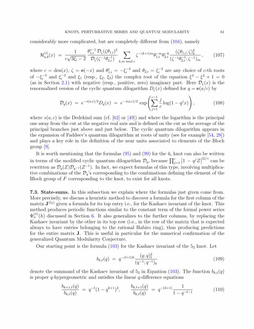
KNOTS, PERTURBATIVE SERIES AND QUANTUM MODULARITY 61
considerably more complicated, but are completely different from (104), namely
H(i)a,b(x) =
1
c√
3ξi − 2
θc−11,i Dζ(ζθ1,i)
2
Dζ(ζ−1θ−12,i )
∑k,m mod c
ζ−(k+1)mθ−m1,i θ−k2,i
(ζθ1,i; ζ)2k
(ζ−1θ−12,i ; ζ
−1)m, (107)
where c = den(x), ζ = e(−x) and θc1,i = −ξ−3i and θ2,i = ξ−2
i are any choice of c-th roots
of −ξ−3i and ξ−2
i and ξ1 (resp., ξ2, ξ3) the complex root of the equation ξ3 − ξ2 + 1 = 0(as in Section 2.1) with negative (resp., positive, zero) imaginary part. Here Dζ(x) is therenormalized version of the cyclic quantum dilogarithm Dζ(x) defined for q = e(a/c) by
Dq(x) = e−s(a,c)/2Dq(x) = e−s(a,c)/2 exp
(c−1∑j=1
j
clog(1− qjx)
), (108)
where s(a, c) is the Dedekind sum (cf. [62] or [49]) and where the logarithm is the principalone away from the cut at the negative real axis and is defined on the cut as the average of theprincipal branches just above and just below. The cyclic quantum dilogarithm appears inthe expansion of Faddeev’s quantum dilogarithm at roots of unity (see for example [54, 28])and plays a key role in the definition of the near units associated to elements of the Blochgroup [9].
It is worth mentioning that the formulas (95) and (99) for the 41 knot can also be written
in terms of the modified cyclic quantum dilogarithm Dq, because∏c
j=1
∣∣1 − qjZ∣∣2j/c can be
rewritten as Dq(Z)Dq−1(Z−1). In fact, we expect formulas of this type, involving multiplica-tive combinations of the Dq’s corresponding to the combinations defining the element of theBloch group of F corresponding to the knot, to exist for all knots.
7.3. State-sums. In this subsection we explain where the formulas just given come from.More precisely, we discuss a heuristic method to discover a formula for the first column of thematrix J(52) given a formula for its top entry i.e., for the Kashaev invariant of the knot. Thismethod produces periodic functions similar to the constant term of the formal power series
Φ(σ)α (h) discussed in Section 6. It also generalizes to the further columns, by replacing the
Kashaev invariant by the other in its top row (i.e., in the row of the matrix that is expectedalways to have entries belonging to the rational Habiro ring), thus producing predictionsfor the entire matrix J. This is useful in particular for the numerical confirmation of thegeneralized Quantum Modularity Conjecture.
Our starting point is the formula (103) for the Kashaev invariant of the 52 knot. Let
bk,`(q) = q−(`+1)k (q; q)2`
(q−1; q−1)k(109)
denote the summand of the Kashaev invariant of 52 in Equation (103). The function bk,`(q)is proper q-hypergeometric and satisfies the linear q-difference equations
bk+1,`(q)
bk,`(q)= q−`(1− qk+1)2,
bk,`+1(q)
bk,`(q)= q−(k+1) 1
1− q−`−1(110)
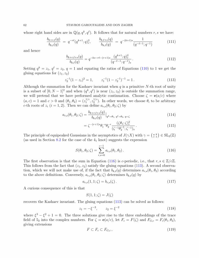
62 STAVROS GAROUFALIDIS AND DON ZAGIER
whose right hand sides are in Q(q, qk, q`). It follows that for natural numbers r, s we have:
bk+r,`(q)
bk,`(q)= q−r`(qk+1; q)2
r,bk,`+s(q)
bk,`(q)= q−(k+1)s 1
(q−`−1; q−1)(111)
and hence
bk+r,`+s(q)
bk,`(q)= q−ks−r`−(r+1)s (qk+1; q)2
r
(q−`−1; q−1)s. (112)
Setting qk = z1, q` = z2, q = 1 and equating the ratios of Equations (110) to 1 we get thegluing equations for (z1, z2)
z−12 (1− z1)2 = 1, z−1
1 (1− z−12 )−1 = 1 . (113)
Although the summation for the Kashaev invariant when q is a primitive N -th root of unityis a subset of [0, N − 1]2 and when (qk, q`) is near (z1, z2) is outside the summation range,we will pretend that we have performed analytic continuation. Choose ζ = e(a/c) where
(a, c) = 1 and c > 0 and (θ1, θ2) = (z1/c1 , z
1/c2 ). In other words, we choose θi to be arbitrary
c-th roots of zi (i = 1, 2). Then we can define ar,s(θ1, θ2; ζ) by
ar,s(θ1, θ2; ζ) =bk+r,`+s(q)
bk,`(q)
∣∣qk=θ1, q`=θ2, q=ζ
(114)
= ζ−(r+1)sθ−s1 θ−r2
(ζθ1; ζ)2r
(ζ−1θ−12 ; ζ−1)s
. (115)
The principle of equipeaked Gaussians in the asymptotics of J(γX) with γ =(a bc s
)∈ SL2(Z)
(as used in Section 8.2 for the case of the 41 knot) suggests the expression
S(θ1, θ2; ζ) =c−1∑r,s=0
ar,s(θ1, θ2) . (116)
The first observation is that the sum in Equation (116) is c-periodic, i.e., that r, s ∈ Z/cZ.This follows from the fact that (z1, z2) satisfy the gluing equations (113). A second observa-tion, which we will not make use of, if the fact that bk,`(q) determines ar,s(θ1, θ2) accordingto the above definitions. Conversely, ar,s(θ1, θ2; ζ) determines bk,`(q) by
ar,s(1, 1; ζ) = br,s(ζ) . (117)
A curious consequence of this is that
S(1, 1; ζ) = J(ζ)
recovers the Kashaev invariant. The gluing equations (113) can be solved as follows:
z1 = −ξ−3, z2 = ξ−2 (118)
where ξ3 − ξ2 + 1 = 0. The three solutions give rise to the three embeddings of the tracefield of 52 into the complex numbers. For ζ = e(a/c), let Fc = F (ζ) and FG,c = Fc(θ1, θ2),giving extensions
F ⊂ Fc ⊂ FG,c , (119)
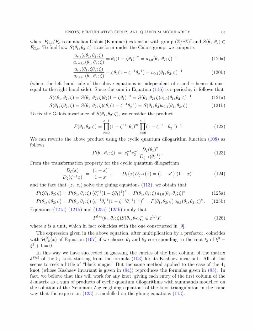
KNOTS, PERTURBATIVE SERIES AND QUANTUM MODULARITY 63
where FG,c/Fc is an abelian Galois (Kummer) extension with group (Z/cZ)2 and S(θ1, θ2) ∈FG,c. To find how S(θ1, θ2; ζ) transform under the Galois group, we compute:
ar,s(ζθ1, θ2; ζ)
ar+1,s(θ1, θ2; ζ)= θ2(1− ζθ1)−2 = a1,0(θ1, θ2; ζ)−1 (120a)
ar,s(θ1, ζθ2; ζ)
ar,s+1(θ1, θ2; ζ)= ζθ1(1− ζ−1θ−1
2 ) = a0,1(θ1, θ2; ζ)−1 (120b)
(where the left hand side of the above equations is independent of r and s hence it mustequal to the right hand side). Since the sum in Equation (116) is c-periodic, it follows that
S(ζθ1, θ2; ζ) = S(θ1, θ2; ζ)θ2(1− ζθ1)−2 = S(θ1, θ2; ζ)a1,0(θ1, θ2; ζ)−1 (121a)
S(θ1, ζθ2; ζ) = S(θ1, θ2; ζ)ζθ1(1− ζ−1θ−12 ) = S(θ1, θ2)a0,1(θ1, θ2; ζ)−1 (121b)
To fix the Galois invariance of S(θ1, θ2; ζ), we consider the product
P (θ1, θ2; ζ) =c−1∏r=0
(1− ζr+1θ1)2r
c−1∏s=0
(1− ζ−s−1θ−12 )−s (122)
We can rewrite the above product using the cyclic quantum dilogarithm function (108) asfollows
P (θ1, θ2; ζ) = z−11 z−1
2
Dζ(θ1)2
Dζ−1(θ−12 )
. (123)
From the transformation property for the cyclic quantum dilogarithm
Dζ(x)
Dζ(ζ−1x)=
(1− x)c
1− xc, Dζ(x)Dζ−1(x) = (1− xc)c(1− x)c (124)
and the fact that (z1, z2) solve the gluing equations (113), we obtain that
P (ζθ1, θ2; ζ) = P (θ1, θ2; ζ)(θ−1
2 (1− ζθ1)2)c
= P (θ1, θ2; ζ) a1,0(θ1, θ2; ζ)c (125a)
P (θ1, ζθ2; ζ) = P (θ1, θ2; ζ)(ζ−1θ−1
1 (1− ζ−1θ−12 )−1
)c= P (θ1, θ2; ζ) a0,1(θ1, θ2; ζ)c . (125b)
Equations (121a)-(121b) and (125a)-(125b) imply that
P 1/c(θ1, θ2; ζ)S(θ1, θ2; ζ) ∈ ε1/cFc (126)
where ε is a unit, which in fact coincides with the one constructed in [9].
The expression given in the above equation, after multiplication by a prefactor, coincides
with H(i)0,0(x) of Equation (107) if we choose θ1 and θ2 corresponding to the root ξi of ξ3 −
ξ2 + 1 = 0.
In this way we have succeeded in guessing the entries of the first column of the matrixJ(52) of the 52 knot starting from the formula (103) for its Kashaev invariant. All of thisseems to reek a little of “black magic.” But the same method applied to the case of the 41
knot (whose Kashaev invariant is given in (94)) reproduces the formulas given in (95). Infact, we believe that this will work for any knot, giving each entry of the first column of theJ-matrix as a sum of products of cyclic quantum dilogarithms with summands modelled onthe solution of the Neumann-Zagier gluing equations of the knot triangulation in the sameway that the expression (123) is modelled on the gluing equations (113).
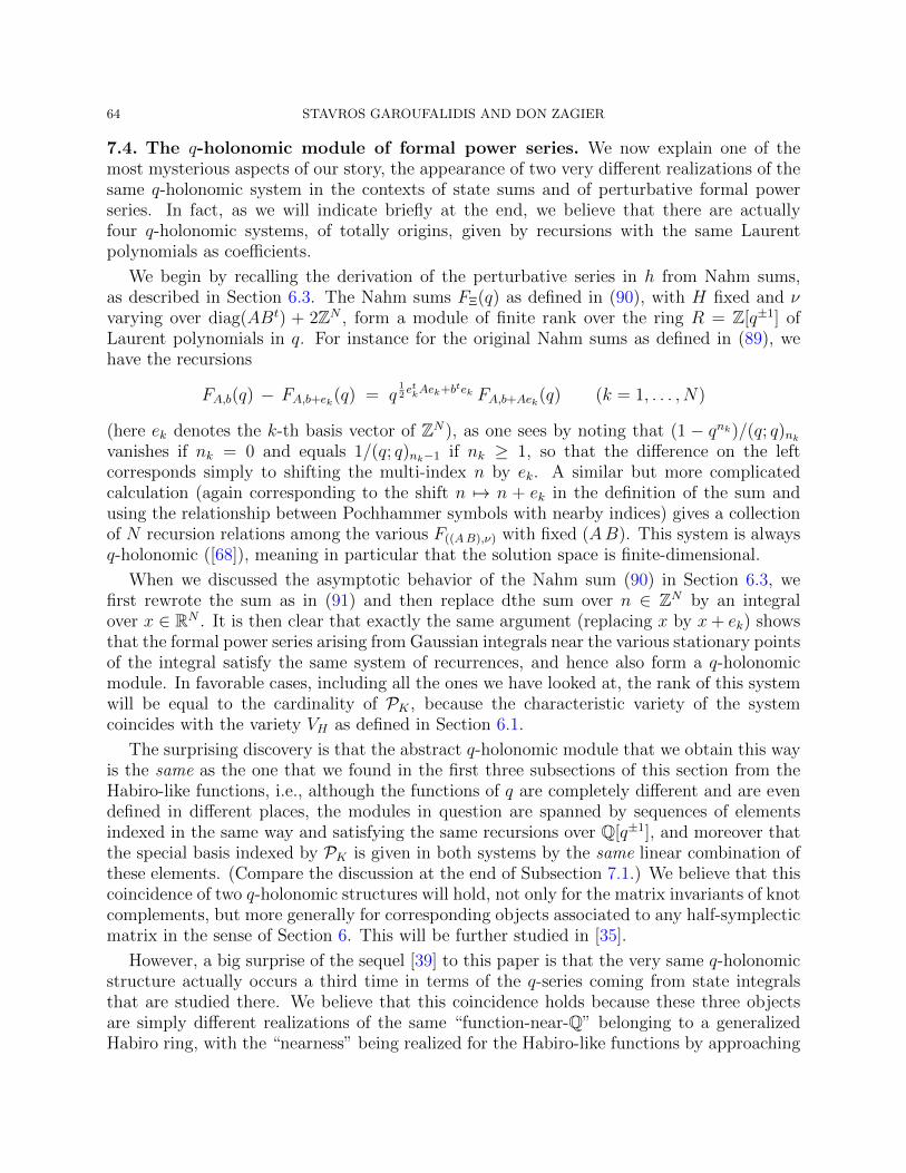
64 STAVROS GAROUFALIDIS AND DON ZAGIER
7.4. The q-holonomic module of formal power series. We now explain one of themost mysterious aspects of our story, the appearance of two very different realizations of thesame q-holonomic system in the contexts of state sums and of perturbative formal powerseries. In fact, as we will indicate briefly at the end, we believe that there are actuallyfour q-holonomic systems, of totally origins, given by recursions with the same Laurentpolynomials as coefficients.
We begin by recalling the derivation of the perturbative series in h from Nahm sums,as described in Section 6.3. The Nahm sums FΞ(q) as defined in (90), with H fixed and νvarying over diag(ABt) + 2ZN , form a module of finite rank over the ring R = Z[q±1] ofLaurent polynomials in q. For instance for the original Nahm sums as defined in (89), wehave the recursions
FA,b(q) − FA,b+ek(q) = q12etkAek+btek FA,b+Aek(q) (k = 1, . . . , N)
(here ek denotes the k-th basis vector of ZN), as one sees by noting that (1 − qnk)/(q; q)nkvanishes if nk = 0 and equals 1/(q; q)nk−1 if nk ≥ 1, so that the difference on the leftcorresponds simply to shifting the multi-index n by ek. A similar but more complicatedcalculation (again corresponding to the shift n 7→ n + ek in the definition of the sum andusing the relationship between Pochhammer symbols with nearby indices) gives a collectionof N recursion relations among the various F((AB),ν) with fixed (AB). This system is alwaysq-holonomic ([68]), meaning in particular that the solution space is finite-dimensional.
When we discussed the asymptotic behavior of the Nahm sum (90) in Section 6.3, wefirst rewrote the sum as in (91) and then replace dthe sum over n ∈ ZN by an integralover x ∈ RN . It is then clear that exactly the same argument (replacing x by x+ ek) showsthat the formal power series arising from Gaussian integrals near the various stationary pointsof the integral satisfy the same system of recurrences, and hence also form a q-holonomicmodule. In favorable cases, including all the ones we have looked at, the rank of this systemwill be equal to the cardinality of PK , because the characteristic variety of the systemcoincides with the variety VH as defined in Section 6.1.
The surprising discovery is that the abstract q-holonomic module that we obtain this wayis the same as the one that we found in the first three subsections of this section from theHabiro-like functions, i.e., although the functions of q are completely different and are evendefined in different places, the modules in question are spanned by sequences of elementsindexed in the same way and satisfying the same recursions over Q[q±1], and moreover thatthe special basis indexed by PK is given in both systems by the same linear combination ofthese elements. (Compare the discussion at the end of Subsection 7.1.) We believe that thiscoincidence of two q-holonomic structures will hold, not only for the matrix invariants of knotcomplements, but more generally for corresponding objects associated to any half-symplecticmatrix in the sense of Section 6. This will be further studied in [35].
However, a big surprise of the sequel [39] to this paper is that the very same q-holonomicstructure actually occurs a third time in terms of the q-series coming from state integralsthat are studied there. We believe that this coincidence holds because these three objectsare simply different realizations of the same “function-near-Q” belonging to a generalizedHabiro ring, with the “nearness” being realized for the Habiro-like functions by approaching
KNOTS, PERTURBATIVE SERIES AND QUANTUM MODULARITY 65
a given rational number through nearby rational numbers of slowly growing height, and inthe case of the q-series by approaching a rational number from above in the upper half-plane(or equivalently, approaching a root of unity radially in the unit disk). We have checked theagreement of the relations over Q[q, q−1] among the columns of the J- and Φ-matrices forboth the 41 and 52 knots (although we do not describe that verification in this paper becausethe specific formulas that were used for J for these two knots in Sections 7.1 and 7.2–7.3 arenot the same as the ones coming from ideal triangulations and Neumann-Zagier data andare rather complicated), while the corresponding verification for the q-series for the sametwo knots is given in [26] and discussed in [39]. We conjecture that these recursive relationscoicide with the ones defined in current work of Rinat Kashaev and the first author [27] fromthe colored Jones polynomials. But we should emphasize that we still have no idea why anyof these q-holonomic modules has a canonical basis indexed by P .
8. Proof of the Modularity Conjecture for the 41 knot
In this section we give our proof of the quantum modularity conjecture for the figure 8knot, announced several years ago. Another proof was given by [5], as well as proofs of thequantum modularity conjecture for a few other knots, but we give our proof for completenessand because the point of view here is somewhat different from the one there.
We denote by J(x) the J-function for the 41 knot, as given explicitly by equation (14)with q = e(x). We have to show that
J(aX + b
cX + d
)∼ (cX + d)3/2 J(X) Φa/c
( 2πi
c(cX + d)
)(127)
to all orders in 1/X as X tends to infinity with bounded denominator with γ =(a bc d
)∈
SL2(Z) fixed and c > 0, where Φa/c(h) = eV/ch Φa/c(h) is the completed version of a formalpower series Φa/c(h) with algebraic coefficients and where V = Vol(S3 r 41) = 2.02988 · · ·is the volume of the complement of this knot. We give the proofs separately for the specialcase γ = S, α := a/c = 0 and for the general case, since all the main ideas are already visiblefor the former and the details are much simpler.
8.1. The case of α = 0. We begin with the case α = 0, which makes it clear where thefactor J(X) in Equation (127) comes from. We use the notation
Pn(x) = |(q)n|2 ,
for q = e(x) with x rational, so that Pn(x) is the n-th summand in the definition of J(x),and denote by cr (r ≥ 0) the numbers defined by the Taylor expansion
cot(π
6− x
2
)=
∞∑r=0
crxr
r!,
the first values being given by the table
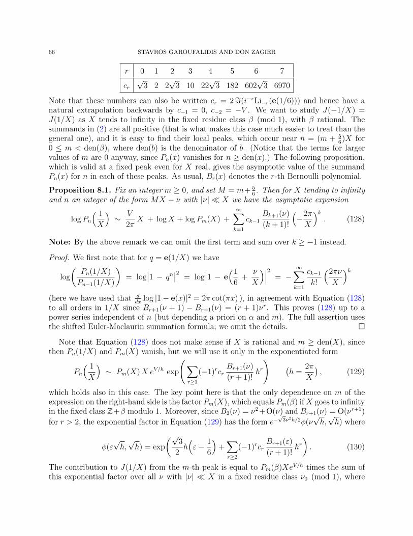
66 STAVROS GAROUFALIDIS AND DON ZAGIER
r 0 1 2 3 4 5 6 7
cr√
3 2 2√
3 10 22√
3 182 602√
3 6970
Note that these numbers can also be written cr = 2=(i−rLi−r(e(1/6))) and hence have anatural extrapolation backwards by c−1 = 0, c−2 = −V . We want to study J(−1/X) =J(1/X) as X tends to infinity in the fixed residue class β (mod 1), with β rational. Thesummands in (2) are all positive (that is what makes this case much easier to treat than thegeneral one), and it is easy to find their local peaks, which occur near n = (m + 5
6)X for
0 ≤ m < den(β), where den(b) is the denominator of b. (Notice that the terms for largervalues of m are 0 anyway, since Pn(x) vanishes for n ≥ den(x).) The following proposition,which is valid at a fixed peak even for X real, gives the asymptotic value of the summandPn(x) for n in each of these peaks. As usual, Br(x) denotes the r-th Bernoulli polynomial.
Proposition 8.1. Fix an integer m ≥ 0, and set M = m+ 56. Then for X tending to infinity
and n an integer of the form MX − ν with |ν| � X we have the asymptotic expansion
logPn
( 1
X
)∼ V
2πX + logX + logPm(X) +
∞∑k=1
ck−1Bk+1(ν)
(k + 1)!
(−2π
X
)k. (128)
Note: By the above remark we can omit the first term and sum over k ≥ −1 instead.
Proof. We first note that for q = e(1/X) we have
log
(Pn(1/X)
Pn−1(1/X)
)= log
∣∣1 − qn∣∣2 = log
∣∣∣1 − e(1
6+
ν
X
)∣∣∣2 = −∞∑k=1
ck−1
k!
(2πν
X
)k(here we have used that d
dxlog |1− e(x)|2 = 2π cot(πx) ), in agreement with Equation (128)
to all orders in 1/X since Br+1(ν + 1) − Br+1(ν) = (r + 1)νr. This proves (128) up to apower series independent of n (but depending a priori on α and m). The full assertion usesthe shifted Euler-Maclaurin summation formula; we omit the details. �
Note that Equation (128) does not make sense if X is rational and m ≥ den(X), sincethen Pn(1/X) and Pm(X) vanish, but we will use it only in the exponentiated form
Pn
( 1
X
)∼ Pm(X)X eV/h exp
(∑r≥1
(−1)rcrBr+1(ν)
(r + 1)!hr
) (h =
2π
X
), (129)
which holds also in this case. The key point here is that the only dependence on m of theexpression on the right-hand side is the factor Pm(X), which equals Pm(β) ifX goes to infinityin the fixed class Z+β modulo 1. Moreover, since B2(ν) = ν2 +O(ν) and Br+1(ν) = O(νr+1)
for r > 2, the exponential factor in Equation (129) has the form e−√
3ν2h/2φ(ν√h,√h) where
φ(ε√h,√h) = exp
(√3
2h(ε− 1
6
)+∑r≥2
(−1)rcrBr+1(ε)
(r + 1)!hr). (130)
The contribution to J(1/X) from the m-th peak is equal to Pm(β)XeV/h times the sum ofthis exponential factor over all ν with |ν| � X in a fixed residue class ν0 (mod 1), where
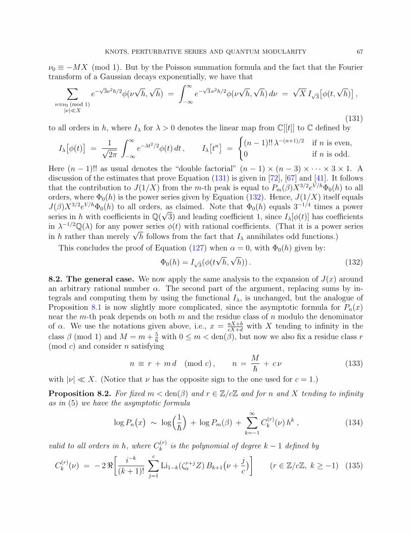
KNOTS, PERTURBATIVE SERIES AND QUANTUM MODULARITY 67
ν0 ≡ −MX (mod 1). But by the Poisson summation formula and the fact that the Fouriertransform of a Gaussian decays exponentially, we have that∑ν≡ν0 (mod 1)|ν|�X
e−√
3ν2h/2φ(ν√h,√h) =
∫ ∞−∞
e−√
3 ν2h/2φ(ν√h,√h) dν =
√X I√3
[φ(t,√h)],
(131)to all orders in h, where Iλ for λ > 0 denotes the linear map from C[[t]] to C defined by
Iλ[φ(t)
]=
1√2π
∫ ∞−∞
e−λt2/2φ(t) dt , Iλ
[tn]
=
{(n− 1)!!λ−(n+1)/2 if n is even,
0 if n is odd.
Here (n − 1)!! as usual denotes the “double factorial” (n − 1) × (n − 3) × · · · × 3 × 1. Adiscussion of the estimates that prove Equation (131) is given in [72], [67] and [41]. It followsthat the contribution to J(1/X) from the m-th peak is equal to Pm(β)X3/2eV/hΦ0(h) to allorders, where Φ0(h) is the power series given by Equation (132). Hence, J(1/X) itself equalsJ(β)X3/2eV/hΦ0(h) to all orders, as claimed. Note that Φ0(h) equals 3−1/4 times a powerseries in h with coefficients in Q(
√3) and leading coefficient 1, since Iλ[φ(t)] has coefficients
in λ−1/2Q(λ) for any power series φ(t) with rational coefficients. (That it is a power series
in h rather than merely√h follows from the fact that Iλ annihilates odd functions.)
This concludes the proof of Equation (127) when α = 0, with Φ0(h) given by:
Φ0(h) = I√3(φ(t√h,√h)) . (132)
8.2. The general case. We now apply the same analysis to the expansion of J(x) aroundan arbitrary rational number α. The second part of the argument, replacing sums by in-tegrals and computing them by using the functional Iλ, is unchanged, but the analogue ofProposition 8.1 is now slightly more complicated, since the asymptotic formula for Pn(x)near the m-th peak depends on both m and the residue class of n modulo the denominatorof α. We use the notations given above, i.e., x = aX+b
cX+dwith X tending to infinity in the
class β (mod 1) and M = m+ 56
with 0 ≤ m < den(β), but now we also fix a residue class r(mod c) and consider n satisfying
n ≡ r + md (mod c) , n =M
~+ c ν (133)
with |ν| � X. (Notice that ν has the opposite sign to the one used for c = 1.)
Proposition 8.2. For fixed m < den(β) and r ∈ Z/cZ and for n and X tending to infinityas in (5) we have the asymptotic formula
logPn(x)∼ log
(1
~
)+ logPm(β) +
∞∑k=−1
C(r)k (ν)hk , (134)
valid to all orders in h, where C(r)k is the polynomial of degree k − 1 defined by
C(r)k (ν) = − 2<
[i−k
(k + 1)!
c∑j=1
Li1−k(ζr+jα Z)Bk+1
(ν +
j
c
)](r ∈ Z/cZ, k ≥ −1) (135)

68 STAVROS GAROUFALIDIS AND DON ZAGIER
with ζα = e(α) and Z = e(−5/(6c)).
The proof of this proposition, which we omit, is similar to that of Proposition 8.1, themain point again being that the difference of the right-hand sides of (134) for n and n − 1is given by
∞∑k=−1
[C
(r)k (ν) − C
(r−1)k (ν − 1)
]hk = − 2<
[∞∑k=0
Li1−k(ζrαZ)
(−ihν)k
k!
]= log
∣∣1 − ζrαZe−iνh∣∣2 = log |1− qn|2
= logPn(x) − logPn−1(x) ,
because
qn = e(n(α − 1
c(cX + d)
))= e
((r +md)α − m+ 5/6
c− ν~
)= ζrαZe
−iνh
and
C(r)k (ν) − C
(r−1)k (ν − 1) = − 2<
[i−k
(k + 1)!
( c∑j=1
−c−1∑j=0
)Li1−k(ζ
r+jα Z)Bk+1
(ν +
j
c
)]
= − 2<[i−kLi1−k(ζ
rαZ)
Bk+1
(ν + 1
)− Bk+1
(ν)
(k + 1)!
]= − 2<
[Li1−k(ζ
rαZ)
(ν/i)k
k!
].
Note that in the above calculation we used that C(r)−1(ν) is independent of both ν and r.
In fact, it is given by
C(r)−1(ν) = 2=
[c∑j=1
Li2(ζr+jα Z)
]=
2
c=[Li2(Zc)
]=
V
c,
where we have used the well-known “distribution” property of the dilogarithm. The corre-
sponding distribution property of the 1-logarithm Li1(z) = − log(1 − z) shows that C(r)0 (ν)
is also independent of ν and is given by
C(r)0 (ν) =
c∑j=1
(ν +
j
c− 1
2
)log∣∣1 − ζr+jα Z
∣∣2 = logEr(α) ,
where Er(α) is the real algebraic number defined by
Er(α) =c∏j=1
∣∣1 − ζr+jα Z∣∣2j/c (r ∈ Z/cZ ) . (136)
Hence the exponentiated version of (6) can be written
Pn(x) ∼ Pm(β)eV/c~
~Er(α) exp
( ∞∑k=1
C(r)k (ν)hk
),
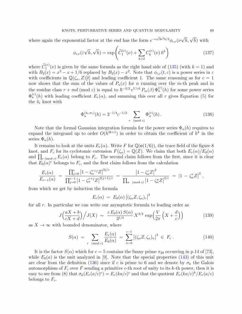
KNOTS, PERTURBATIVE SERIES AND QUANTUM MODULARITY 69
where again the exponential factor at the end has the form e−c√
3ν2h/2φc,r(ν√h,√h) with
φc,r(ε√h,√h) = exp
(C
(r)1 (ν) +
∑k≥2
C(r)k (ν)hk
)(137)
where C(r)1 (ν) is given by the same formula as the right hand side of (135) (with k = 1) and
with B2(x) = x2 − x+ 1/6 replaced by B2(x)− x2. Note that φc,r(t, ε) is a power series in εwith coefficients in Q(ζα, Z)[t] and leading coefficient 1. The same reasoning as for c = 1now shows that the sum of the values of Pn(x) for n running over the m-th peak and in
the residue class r + md (mod c) is equal to ~−3/2 eV/c~ Pm(β) Φ(r)α (h) for some power series
Φ(r)a (h) with leading coefficient Er(α), and summing this over all r gives Equation (5) for
the 41 knot with
Φ(41,σ1)α (h) = 3−1/4c−1/2
∑r (mod c)
Φ(r)α (h) . (138)
Note that the formal Gaussian integration formula for the power series Φα(h) requires toexpand the integrand up to order O(h3k+1) in order to obtain the coefficient of hk in theseries Φα(h).
It remains to look at the units Er(α). Write F for Q(e(1/6)), the trace field of the figure 8knot, and Fc for its cyclotomic extension F (ζα) = Q(Z). We claim that both Er(α)/E0(α)and
∏r (mod c) Er(α) belong to Fc. The second claim follows from the first, since it is clear
that E0(α)c belongs to Fc, and the first claim follows from the calculation
Er(α)
Er−1(α)=
∏cj=0
∣∣1− ζr+jα Z∣∣2j/c∏c−1
j=0
∣∣1− ζr+jα Z∣∣2(j+1)/c
=
∣∣1− ζrαZ∣∣2∏n (mod c)
∣∣1− ζnαZ∣∣2/c = |1 − ζrαZ∣∣2 ,
from which we get by induction the formula
Er(α) = E0(α)∣∣(ζαZ, ζα)r
∣∣2for all r. In particular we can write our asymptotic formula to leading order as
J(aX + b
cX + d
)/J(X) ∼ cE0(α)S(α)
31/4X3/2 exp
( V2π
(X +
d
c
))(139)
as X →∞ with bounded denominator, where
S(α) =∑
r (mod c)
Er(α)
E0(α)=
c−1∑n=0
∣∣(ζαZ, ζα)n∣∣2 ∈ Fc . (140)
It is the factor S(α) which for c = 5 contains the funny prime π29 occurring in p.14 of [73],while E0(a) is the unit analyzed in [9]. Note that the special properties (143) of this unitare clear from the definition (136) since if c is prime to 6 and we denote by σk the Galoisautomorphism of Fc over F sending a primitive c-th root of unity to its k-th power, then it iseasy to see from (8) that σk(Er(a/c)
c) = Er(ka/c)c and that the quotient Er(ka/c)
k/Er(a/c)belongs to Fc.
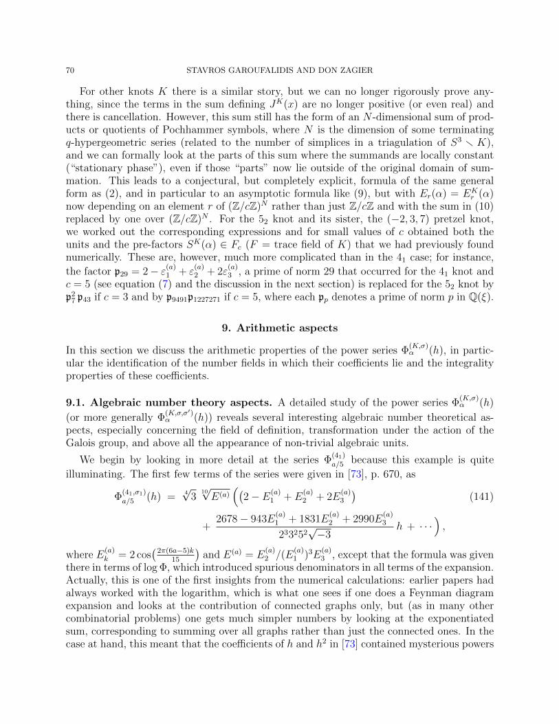
70 STAVROS GAROUFALIDIS AND DON ZAGIER
For other knots K there is a similar story, but we can no longer rigorously prove any-thing, since the terms in the sum defining JK(x) are no longer positive (or even real) andthere is cancellation. However, this sum still has the form of an N -dimensional sum of prod-ucts or quotients of Pochhammer symbols, where N is the dimension of some terminatingq-hypergeometric series (related to the number of simplices in a triagulation of S3 r K),and we can formally look at the parts of this sum where the summands are locally constant(“stationary phase”), even if those “parts” now lie outside of the original domain of sum-mation. This leads to a conjectural, but completely explicit, formula of the same generalform as (2), and in particular to an asymptotic formula like (9), but with Er(α) = EK
r (α)now depending on an element r of (Z/cZ)N rather than just Z/cZ and with the sum in (10)replaced by one over (Z/cZ)N . For the 52 knot and its sister, the (−2, 3, 7) pretzel knot,we worked out the corresponding expressions and for small values of c obtained both theunits and the pre-factors SK(α) ∈ Fc (F = trace field of K) that we had previously foundnumerically. These are, however, much more complicated than in the 41 case; for instance,
the factor p29 = 2− ε(a)1 + ε
(a)2 + 2ε
(a)3 , a prime of norm 29 that occurred for the 41 knot and
c = 5 (see equation (7) and the discussion in the next section) is replaced for the 52 knot byp2
7 p43 if c = 3 and by p9491p1227271 if c = 5, where each pp denotes a prime of norm p in Q(ξ).
9. Arithmetic aspects
In this section we discuss the arithmetic properties of the power series Φ(K,σ)α (h), in partic-
ular the identification of the number fields in which their coefficients lie and the integralityproperties of these coefficients.
9.1. Algebraic number theory aspects. A detailed study of the power series Φ(K,σ)α (h)
(or more generally Φ(K,σ,σ′)α (h)) reveals several interesting algebraic number theoretical as-
pects, especially concerning the field of definition, transformation under the action of theGalois group, and above all the appearance of non-trivial algebraic units.
We begin by looking in more detail at the series Φ(41)a/5 because this example is quite
illuminating. The first few terms of the series were given in [73], p. 670, as
Φ(41,σ1)a/5 (h) =
4√
310√E(a)
((2− E(a)
1 + E(a)2 + 2E
(a)3
)(141)
+2678− 943E
(a)1 + 1831E
(a)2 + 2990E
(a)3
233252√−3
h + · · ·),
where E(a)k = 2 cos
(2π(6a−5)k15
)and E(a) = E
(a)2 /(E
(a)1 )3E
(a)3 , except that the formula was given
there in terms of log Φ, which introduced spurious denominators in all terms of the expansion.Actually, this is one of the first insights from the numerical calculations: earlier papers hadalways worked with the logarithm, which is what one sees if one does a Feynman diagramexpansion and looks at the contribution of connected graphs only, but (as in many othercombinatorial problems) one gets much simpler numbers by looking at the exponentiatedsum, corresponding to summing over all graphs rather than just the connected ones. In thecase at hand, this meant that the coefficients of h and h2 in [73] contained mysterious powers
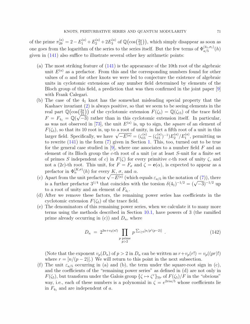
KNOTS, PERTURBATIVE SERIES AND QUANTUM MODULARITY 71
of the prime π(a)29 = 2−E(a)
1 +E(a)2 + 2E
(a)3 of Q
(cos(
2π15
)), which simply disappear as soon as
one goes from the logarithm of the series to the series itself. But the few terms of Φ(41,σ1)a/5 (h)
given in (141) also suffice to illustrate several other key arithmetic points:
(a) The most striking feature of (141) is the appearance of the 10th root of the algebraicunit E(a) as a prefactor. From this and the corresponding numbers found for othervalues of α and for other knots we were led to conjecture the existence of algebraicunits in cyclotomic extensions of any number field determined by elements of theBloch group of this field, a prediction that was then confirmed in the joint paper [9]with Frank Calegari.
(b) The case of the 41 knot has the somewhat misleading special property that theKashaev invariant (2) is always positive, so that we seem to be seeing elements in thereal part Q
(cos(
2π15
))of the cyclotomic extension F (ζ5) = Q(ζ15) of the trace field
F = F41 = Q(√−3) rather than in this cyclotomic extension itself. In particular,
as was not observed in [73], the unit E(a) is, up to sign, the square of an element ofF (ζ5), so that its 10 root is, up to a root of unity, in fact a fifth root of a unit in this
larger field. Specifically, we have√−E(a) = (ζ
(a)15 − (ζ
(a)15 )−1)E
(a)2 /E
(a)1 , permitting us
to rewrite (141) in the form (7) given in Section 1. This, too, turned out to be truefor the general case studied in [9], where one associates to a number field F and anelement of its Bloch group the c-th root of a unit (or at least S-unit for a finite setof primes S independent of c) in F (ζ) for every primitive c-th root of unity ζ, andnot a (2c)-th root. This unit, for F = Fσ and ζ = e(α), is expected to appear as a
prefactor in Φ(K,σ)α (h) for every K, σ, and α.
(c) Apart from the unit prefactor√−E(a) (which equals εa/5 in the notation of (7)), there
is a further prefactor 31/4 that coincides with the torsion δ(41)−1/2 = (√−3)−1/2 up
to a root of unity and an element of F41 .(d) After we remove these factors, the remaining power series has coefficients in the
cyclotomic extension F (ζ5) of the trace field.(e) The denominators of this remaining power series, when we calculate it to many more
terms using the methods described in Section 10.1, have powers of 3 (the ramifiedprime already occurring in (c)) and Dn, where
Dn = 23n+v2(n!)∏
p primep>2
p∑i≥0[n/pi(p−2)] . (142)
(Note that the exponent vp(Dn) of p > 2 in Dn can be written as r+vp(r!) = vp((pr)!)where r = [n/(p− 2)].) We will return to this point in the next subsection.
(f) The unit εa/5 occurring in (a) and (b), the term under the square-root sign in (c),and the coefficients of the “remaining power series” as defined in (d) are not only inF (ζ5), but transform under the Galois group {ζ 7→ ζr}5-r of F (ζ5)/F in the “obvious”
way, i.e., each of these numbers is a polynomial in ζ = e2πia/5 whose coefficients liein F41 and are independent of a.
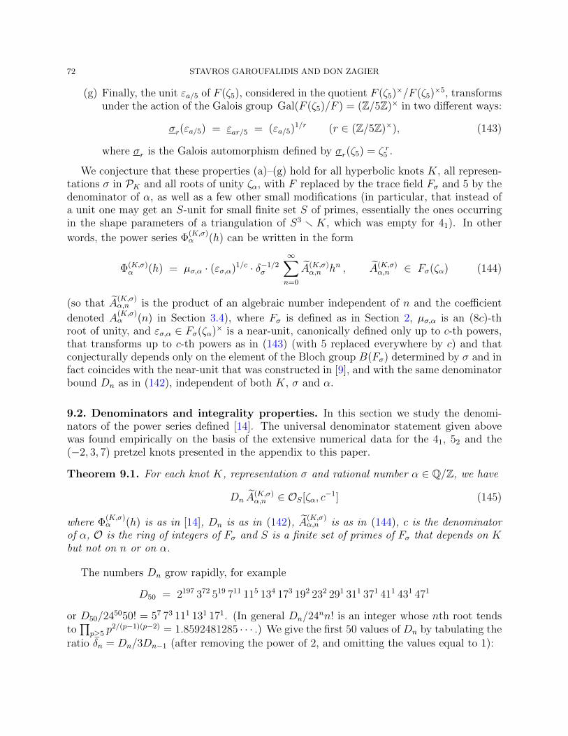
72 STAVROS GAROUFALIDIS AND DON ZAGIER
(g) Finally, the unit εa/5 of F (ζ5), considered in the quotient F (ζ5)×/F (ζ5)×5, transformsunder the action of the Galois group Gal(F (ζ5)/F ) = (Z/5Z)× in two different ways:
σr(εa/5) = εar/5 = (εa/5)1/r (r ∈ (Z/5Z)×), (143)
where σr is the Galois automorphism defined by σr(ζ5) = ζ r5 .
We conjecture that these properties (a)–(g) hold for all hyperbolic knots K, all represen-tations σ in PK and all roots of unity ζα, with F replaced by the trace field Fσ and 5 by thedenominator of α, as well as a few other small modifications (in particular, that instead ofa unit one may get an S-unit for small finite set S of primes, essentially the ones occurringin the shape parameters of a triangulation of S3 r K, which was empty for 41). In other
words, the power series Φ(K,σ)α (h) can be written in the form
Φ(K,σ)α (h) = µσ,α · (εσ,α)1/c · δ−1/2
σ
∞∑n=0
A(K,σ)α,n hn , A(K,σ)
α,n ∈ Fσ(ζα) (144)
(so that A(K,σ)α,n is the product of an algebraic number independent of n and the coefficient
denoted A(K,σ)α (n) in Section 3.4), where Fσ is defined as in Section 2, µσ,α is an (8c)-th
root of unity, and εσ,α ∈ Fσ(ζα)× is a near-unit, canonically defined only up to c-th powers,that transforms up to c-th powers as in (143) (with 5 replaced everywhere by c) and thatconjecturally depends only on the element of the Bloch group B(Fσ) determined by σ and infact coincides with the near-unit that was constructed in [9], and with the same denominatorbound Dn as in (142), independent of both K, σ and α.
9.2. Denominators and integrality properties. In this section we study the denomi-nators of the power series defined [14]. The universal denominator statement given abovewas found empirically on the basis of the extensive numerical data for the 41, 52 and the(−2, 3, 7) pretzel knots presented in the appendix to this paper.
Theorem 9.1. For each knot K, representation σ and rational number α ∈ Q/Z, we have
Dn A(K,σ)α,n ∈ OS[ζα, c
−1] (145)
where Φ(K,σ)α (h) is as in [14], Dn is as in (142), A
(K,σ)α,n is as in (144), c is the denominator
of α, O is the ring of integers of Fσ and S is a finite set of primes of Fσ that depends on Kbut not on n or on α.
The numbers Dn grow rapidly, for example
D50 = 2197 372 519 711 115 134 173 192 232 291 311 371 411 431 471
or D50/245050! = 57 73 111 131 171. (In general Dn/24nn! is an integer whose nth root tendsto∏
p≥5 p2/(p−1)(p−2) = 1.8592481285 · · · .) We give the first 50 values of Dn by tabulating the
ratio δn = Dn/3Dn−1 (after removing the power of 2, and omitting the values equal to 1):
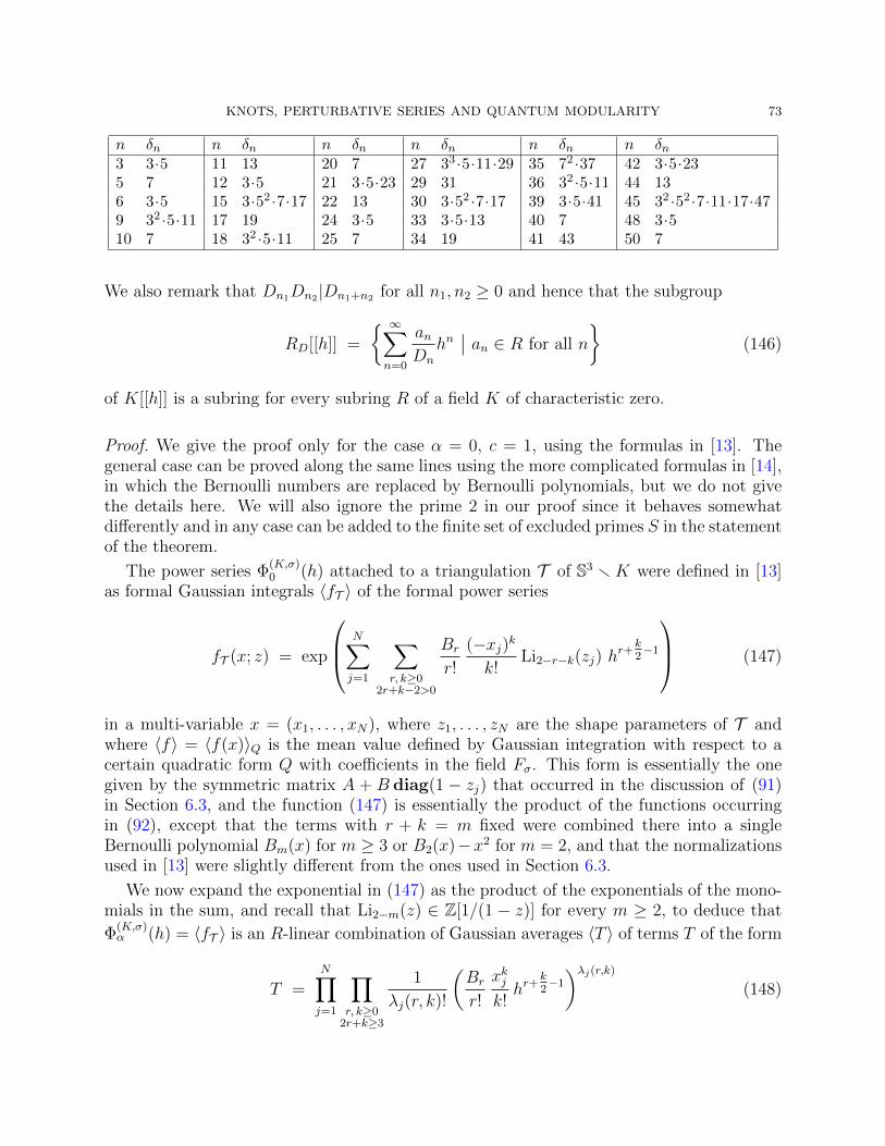
KNOTS, PERTURBATIVE SERIES AND QUANTUM MODULARITY 73
n δn n δn n δn n δn n δn n δn3 3·5 11 13 20 7 27 33 ·5·11·29 35 72 ·37 42 3·5·235 7 12 3·5 21 3·5·23 29 31 36 32 ·5·11 44 136 3·5 15 3·52 ·7·17 22 13 30 3·52 ·7·17 39 3·5·41 45 32 ·52 ·7·11·17·479 32 ·5·11 17 19 24 3·5 33 3·5·13 40 7 48 3·510 7 18 32 ·5·11 25 7 34 19 41 43 50 7
We also remark that Dn1Dn2|Dn1+n2 for all n1, n2 ≥ 0 and hence that the subgroup
RD[[h]] =
{ ∞∑n=0
anDn
hn∣∣ an ∈ R for all n
}(146)
of K[[h]] is a subring for every subring R of a field K of characteristic zero.
Proof. We give the proof only for the case α = 0, c = 1, using the formulas in [13]. Thegeneral case can be proved along the same lines using the more complicated formulas in [14],in which the Bernoulli numbers are replaced by Bernoulli polynomials, but we do not givethe details here. We will also ignore the prime 2 in our proof since it behaves somewhatdifferently and in any case can be added to the finite set of excluded primes S in the statementof the theorem.
The power series Φ(K,σ)0 (h) attached to a triangulation T of S3 rK were defined in [13]
as formal Gaussian integrals 〈fT 〉 of the formal power series
fT (x; z) = exp
N∑j=1
∑r, k≥0
2r+k−2>0
Br
r!
(−xj)k
k!Li2−r−k(zj) h
r+k2−1
(147)
in a multi-variable x = (x1, . . . , xN), where z1, . . . , zN are the shape parameters of T andwhere 〈f〉 = 〈f(x)〉Q is the mean value defined by Gaussian integration with respect to acertain quadratic form Q with coefficients in the field Fσ. This form is essentially the onegiven by the symmetric matrix A + B diag(1 − zj) that occurred in the discussion of (91)in Section 6.3, and the function (147) is essentially the product of the functions occurringin (92), except that the terms with r + k = m fixed were combined there into a singleBernoulli polynomial Bm(x) for m ≥ 3 or B2(x)−x2 for m = 2, and that the normalizationsused in [13] were slightly different from the ones used in Section 6.3.
We now expand the exponential in (147) as the product of the exponentials of the mono-mials in the sum, and recall that Li2−m(z) ∈ Z[1/(1 − z)] for every m ≥ 2, to deduce that
Φ(K,σ)α (h) = 〈fT 〉 is an R-linear combination of Gaussian averages 〈T 〉 of terms T of the form
T =N∏j=1
∏r, k≥0
2r+k≥3
1
λj(r, k)!
(Br
r!
xkjk!hr+
k2−1
)λj(r,k)
(148)
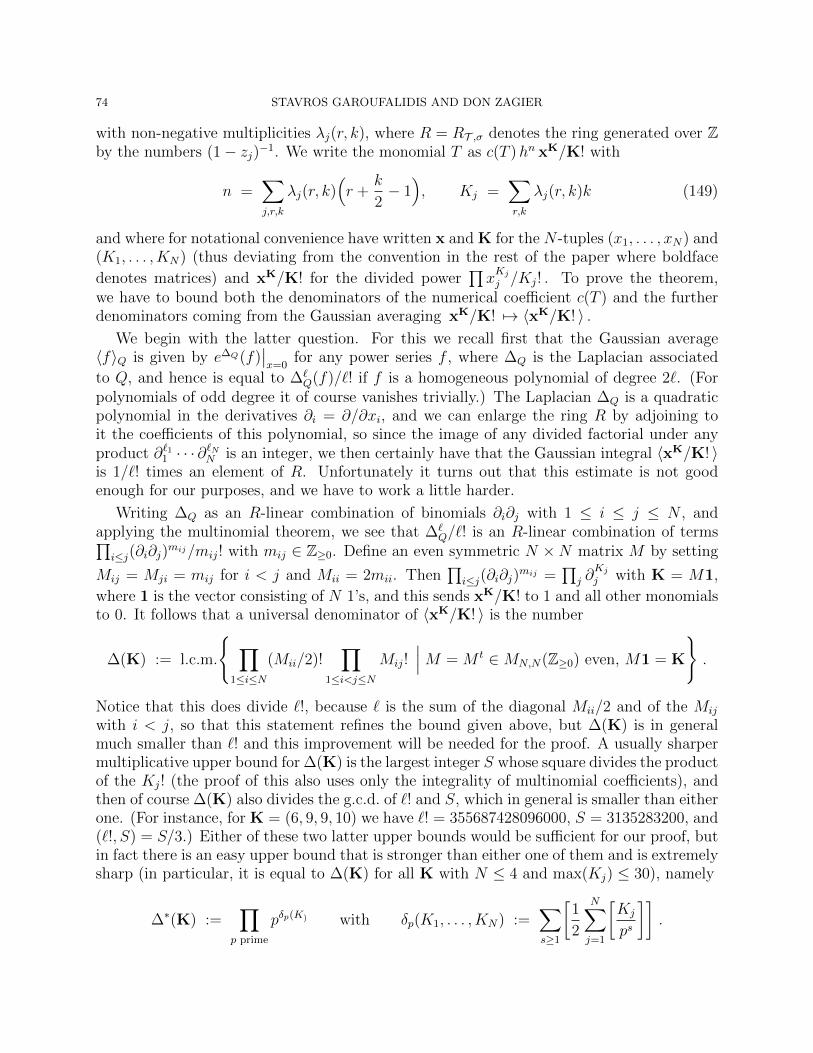
74 STAVROS GAROUFALIDIS AND DON ZAGIER
with non-negative multiplicities λj(r, k), where R = RT ,σ denotes the ring generated over Zby the numbers (1− zj)−1. We write the monomial T as c(T )hn xK/K! with
n =∑j,r,k
λj(r, k)(r +
k
2− 1), Kj =
∑r,k
λj(r, k)k (149)
and where for notational convenience have written x and K for the N -tuples (x1, . . . , xN) and(K1, . . . , KN) (thus deviating from the convention in the rest of the paper where boldface
denotes matrices) and xK/K! for the divided power∏xKjj /Kj! . To prove the theorem,
we have to bound both the denominators of the numerical coefficient c(T ) and the furtherdenominators coming from the Gaussian averaging xK/K! 7→ 〈xK/K! 〉 .
We begin with the latter question. For this we recall first that the Gaussian average〈f〉Q is given by e∆Q(f)
∣∣x=0
for any power series f , where ∆Q is the Laplacian associated
to Q, and hence is equal to ∆`Q(f)/`! if f is a homogeneous polynomial of degree 2`. (For
polynomials of odd degree it of course vanishes trivially.) The Laplacian ∆Q is a quadraticpolynomial in the derivatives ∂i = ∂/∂xi, and we can enlarge the ring R by adjoining toit the coefficients of this polynomial, so since the image of any divided factorial under anyproduct ∂`11 · · · ∂
`NN is an integer, we then certainly have that the Gaussian integral 〈xK/K! 〉
is 1/`! times an element of R. Unfortunately it turns out that this estimate is not goodenough for our purposes, and we have to work a little harder.
Writing ∆Q as an R-linear combination of binomials ∂i∂j with 1 ≤ i ≤ j ≤ N , andapplying the multinomial theorem, we see that ∆`
Q/`! is an R-linear combination of terms∏i≤j(∂i∂j)
mij/mij! with mij ∈ Z≥0. Define an even symmetric N ×N matrix M by setting
Mij = Mji = mij for i < j and Mii = 2mii. Then∏
i≤j(∂i∂j)mij =
∏j ∂
Kjj with K = M1,
where 1 is the vector consisting of N 1’s, and this sends xK/K! to 1 and all other monomialsto 0. It follows that a universal denominator of 〈xK/K! 〉 is the number
∆(K) := l.c.m.
{ ∏1≤i≤N
(Mii/2)!∏
1≤i<j≤N
Mij!∣∣∣M = M t ∈MN,N(Z≥0) even, M1 = K
}.
Notice that this does divide `!, because ` is the sum of the diagonal Mii/2 and of the Mij
with i < j, so that this statement refines the bound given above, but ∆(K) is in generalmuch smaller than `! and this improvement will be needed for the proof. A usually sharpermultiplicative upper bound for ∆(K) is the largest integer S whose square divides the productof the Kj! (the proof of this also uses only the integrality of multinomial coefficients), andthen of course ∆(K) also divides the g.c.d. of `! and S, which in general is smaller than eitherone. (For instance, for K = (6, 9, 9, 10) we have `! = 355687428096000, S = 3135283200, and(`!, S) = S/3.) Either of these two latter upper bounds would be sufficient for our proof, butin fact there is an easy upper bound that is stronger than either one of them and is extremelysharp (in particular, it is equal to ∆(K) for all K with N ≤ 4 and max(Kj) ≤ 30), namely
∆∗(K) :=∏
p prime
pδp(K) with δp(K1, . . . , KN) :=∑s≥1
[1
2
N∑j=1
[Kj
ps
]].
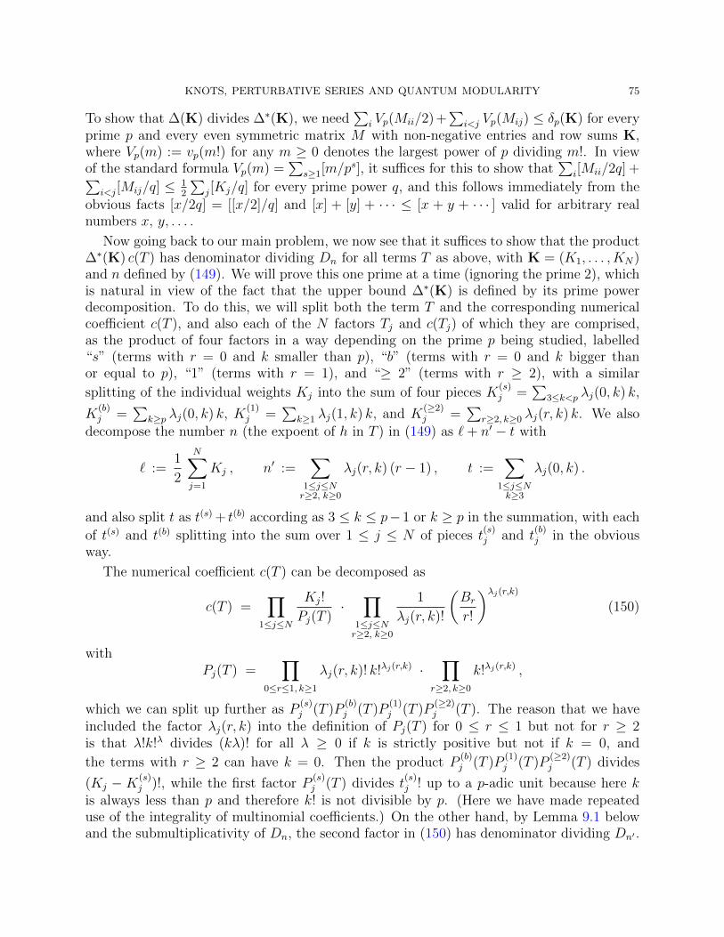
KNOTS, PERTURBATIVE SERIES AND QUANTUM MODULARITY 75
To show that ∆(K) divides ∆∗(K), we need∑
i Vp(Mii/2) +∑
i<j Vp(Mij) ≤ δp(K) for everyprime p and every even symmetric matrix M with non-negative entries and row sums K,where Vp(m) := vp(m!) for any m ≥ 0 denotes the largest power of p dividing m!. In viewof the standard formula Vp(m) =
∑s≥1[m/ps], it suffices for this to show that
∑i[Mii/2q] +∑
i<j[Mij/q] ≤ 12
∑j[Kj/q] for every prime power q, and this follows immediately from the
obvious facts [x/2q] = [[x/2]/q] and [x] + [y] + · · · ≤ [x + y + · · · ] valid for arbitrary realnumbers x, y, . . . .
Now going back to our main problem, we now see that it suffices to show that the product∆∗(K) c(T ) has denominator dividing Dn for all terms T as above, with K = (K1, . . . , KN)and n defined by (149). We will prove this one prime at a time (ignoring the prime 2), whichis natural in view of the fact that the upper bound ∆∗(K) is defined by its prime powerdecomposition. To do this, we will split both the term T and the corresponding numericalcoefficient c(T ), and also each of the N factors Tj and c(Tj) of which they are comprised,as the product of four factors in a way depending on the prime p being studied, labelled“s” (terms with r = 0 and k smaller than p), “b” (terms with r = 0 and k bigger thanor equal to p), “1” (terms with r = 1), and “≥ 2” (terms with r ≥ 2), with a similar
splitting of the individual weights Kj into the sum of four pieces K(s)j =
∑3≤k<p λj(0, k) k,
K(b)j =
∑k≥p λj(0, k) k, K
(1)j =
∑k≥1 λj(1, k) k, and K
(≥2)j =
∑r≥2, k≥0 λj(r, k) k. We also
decompose the number n (the expoent of h in T ) in (149) as `+ n′ − t with
` :=1
2
N∑j=1
Kj , n′ :=∑
1≤j≤Nr≥2, k≥0
λj(r, k) (r − 1) , t :=∑
1≤j≤Nk≥3
λj(0, k) .
and also split t as t(s) + t(b) according as 3 ≤ k ≤ p− 1 or k ≥ p in the summation, with each
of t(s) and t(b) splitting into the sum over 1 ≤ j ≤ N of pieces t(s)j and t
(b)j in the obvious
way.
The numerical coefficient c(T ) can be decomposed as
c(T ) =∏
1≤j≤N
Kj!
Pj(T )·
∏1≤j≤Nr≥2, k≥0
1
λj(r, k)!
(Br
r!
)λj(r,k)
(150)
withPj(T ) =
∏0≤r≤1, k≥1
λj(r, k)! k!λj(r,k) ·∏
r≥2, k≥0
k!λj(r,k) ,
which we can split up further as P(s)j (T )P
(b)j (T )P
(1)j (T )P
(≥2)j (T ). The reason that we have
included the factor λj(r, k) into the definition of Pj(T ) for 0 ≤ r ≤ 1 but not for r ≥ 2is that λ!k!λ divides (kλ)! for all λ ≥ 0 if k is strictly positive but not if k = 0, and
the terms with r ≥ 2 can have k = 0. Then the product P(b)j (T )P
(1)j (T )P
(≥2)j (T ) divides
(Kj − K(s)j )!, while the first factor P
(s)j (T ) divides t
(s)j ! up to a p-adic unit because here k
is always less than p and therefore k! is not divisible by p. (Here we have made repeateduse of the integrality of multinomial coefficients.) On the other hand, by Lemma 9.1 belowand the submultiplicativity of Dn, the second factor in (150) has denominator dividing Dn′ .
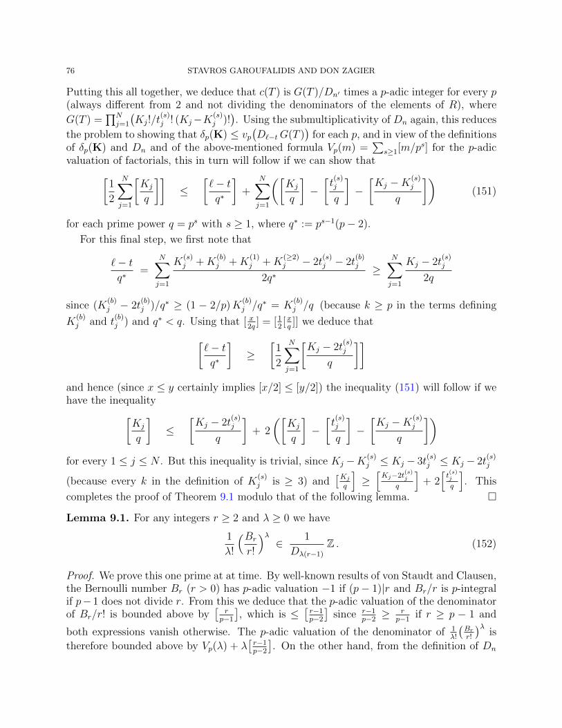
76 STAVROS GAROUFALIDIS AND DON ZAGIER
Putting this all together, we deduce that c(T ) is G(T )/Dn′ times a p-adic integer for every p(always different from 2 and not dividing the denominators of the elements of R), where
G(T ) =∏N
j=1
(Kj!/t
(s)j ! (Kj−K(s)
j )!). Using the submultiplicativity of Dn again, this reduces
the problem to showing that δp(K) ≤ vp(D`−tG(T )
)for each p, and in view of the definitions
of δp(K) and Dn and of the above-mentioned formula Vp(m) =∑
s≥1[m/ps] for the p-adicvaluation of factorials, this in turn will follow if we can show that[
1
2
N∑j=1
[Kj
q
]]≤
[`− tq∗
]+
N∑j=1
([Kj
q
]−[t(s)j
q
]−[Kj −K(s)
j
q
])(151)
for each prime power q = ps with s ≥ 1, where q∗ := ps−1(p− 2).
For this final step, we first note that
`− tq∗
=N∑j=1
K(s)j +K
(b)j +K
(1)j +K
(≥2)j − 2t
(s)j − 2t
(b)j
2q∗≥
N∑j=1
Kj − 2t(s)j
2q
since (K(b)j − 2t
(b)j )/q∗ ≥ (1 − 2/p)K
(b)j /q∗ = K
(b)j /q (because k ≥ p in the terms defining
K(b)j and t
(b)j ) and q∗ < q. Using that [ x
2q] = [1
2[xq]] we deduce that[
`− tq∗
]≥
[1
2
N∑j=1
[Kj − 2t
(s)j
q
]]and hence (since x ≤ y certainly implies [x/2] ≤ [y/2]) the inequality (151) will follow if wehave the inequality[
Kj
q
]≤
[Kj − 2t
(s)j
q
]+ 2
([Kj
q
]−[t(s)j
q
]−[Kj −K(s)
j
q
])for every 1 ≤ j ≤ N . But this inequality is trivial, since Kj −K(s)
j ≤ Kj − 3t(s)j ≤ Kj − 2t
(s)j
(because every k in the definition of K(s)j is ≥ 3) and
[Kjq
]≥[Kj−2t
(s)j
q
]+ 2[t(s)j
q
]. This
completes the proof of Theorem 9.1 modulo that of the following lemma. �
Lemma 9.1. For any integers r ≥ 2 and λ ≥ 0 we have
1
λ!
(Br
r!
)λ∈ 1
Dλ(r−1)
Z . (152)
Proof. We prove this one prime at at time. By well-known results of von Staudt and Clausen,the Bernoulli number Br (r > 0) has p-adic valuation −1 if (p− 1)|r and Br/r is p-integralif p− 1 does not divide r. From this we deduce that the p-adic valuation of the denominatorof Br/r! is bounded above by
[rp−1
], which is ≤
[r−1p−2
]since r−1
p−2≥ r
p−1if r ≥ p − 1 and
both expressions vanish otherwise. The p-adic valuation of the denominator of 1λ!
(Brr!
)λis
therefore bounded above by Vp(λ) + λ[r−1p−2
]. On the other hand, from the definition of Dn
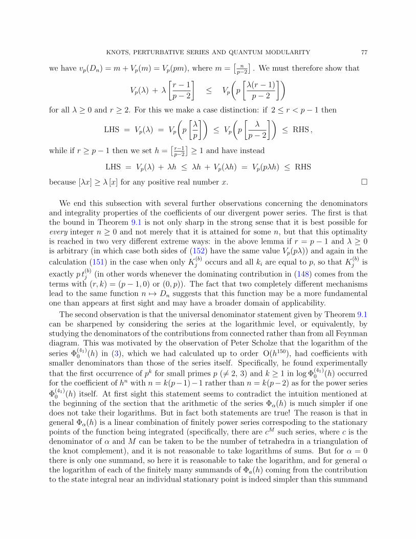
KNOTS, PERTURBATIVE SERIES AND QUANTUM MODULARITY 77
we have vp(Dn) = m+ Vp(m) = Vp(pm), where m =[
np−2
]. We must therefore show that
Vp(λ) + λ
[r − 1
p− 2
]≤ Vp
(p
[λ(r − 1)
p− 2
])for all λ ≥ 0 and r ≥ 2. For this we make a case distinction: if 2 ≤ r < p− 1 then
LHS = Vp(λ) = Vp
(p
[λ
p
])≤ Vp
(p
[λ
p− 2
])≤ RHS ,
while if r ≥ p− 1 then we set h =[r−1p−2
]≥ 1 and have instead
LHS = Vp(λ) + λh ≤ λh + Vp(λh) = Vp(pλh) ≤ RHS
because [λx] ≥ λ [x] for any positive real number x. �
We end this subsection with several further observations concerning the denominatorsand integrality properties of the coefficients of our divergent power series. The first is thatthe bound in Theorem 9.1 is not only sharp in the strong sense that it is best possible forevery integer n ≥ 0 and not merely that it is attained for some n, but that this optimalityis reached in two very different extreme ways: in the above lemma if r = p − 1 and λ ≥ 0is arbitrary (in which case both sides of (152) have the same value Vp(pλ)) and again in the
calculation (151) in the case when only K(b)j occurs and all ki are equal to p, so that K
(b)j is
exactly p t(b)j (in other words whenever the dominating contribution in (148) comes from the
terms with (r, k) = (p− 1, 0) or (0, p)). The fact that two completely different mechanismslead to the same function n 7→ Dn suggests that this function may be a more fundamentalone than appears at first sight and may have a broader domain of applicability.
The second observation is that the universal denominator statement given by Theorem 9.1can be sharpened by considering the series at the logarithmic level, or equivalently, bystudying the denominators of the contributions from connected rather than from all Feynmandiagram. This was motivated by the observation of Peter Scholze that the logarithm of the
series Φ(41)0 (h) in (3), which we had calculated up to order O(h150), had coefficients with
smaller denominators than those of the series itself. Specifically, he found experimentally
that the first occurrence of pk for small primes p ( 6= 2, 3) and k ≥ 1 in log Φ(41)0 (h) occurred
for the coefficient of hn with n = k(p−1)−1 rather than n = k(p−2) as for the power series
Φ(41)0 (h) itself. At first sight this statement seems to contradict the intuition mentioned at
the beginning of the section that the arithmetic of the series Φα(h) is much simpler if onedoes not take their logarithms. But in fact both statements are true! The reason is that ingeneral Φα(h) is a linear combination of finitely power series correspoding to the stationarypoints of the function being integrated (specifically, there are cM such series, where c is thedenominator of α and M can be taken to be the number of tetrahedra in a triangulation ofthe knot complement), and it is not reasonable to take logarithms of sums. But for α = 0there is only one summand, so here it is reasonable to take the logarithm, and for general αthe logarithm of each of the finitely many summands of Φa(h) coming from the contributionto the state integral near an individual stationary point is indeed simpler than this summand
78 STAVROS GAROUFALIDIS AND DON ZAGIER
itself, because it corresponds to a sum over only connected rather than over all Feynmandiagrams. The final statement is given in the following theorem.
Theorem 9.2. For each integer n ≥ 1 define
Dconnn =
∏p prime
p[(n+1)/(p−1)] . (153)
Then the coefficient of hn in log Φ(K,σ)0 (h) for any knot K and any σ ∈ PK has denominator
dividing Dconnn apart from a finite set of primes depending only on K and σ. More generally,
for any α ∈ Q we have Φ(K,σ)α (h) ∈ R⊗ exp
(∑n≥1Rh
n/Dconnn
).
[The proof is still in progress, but the main steps are in place and the statement has also
been checked numerically for the first 200 coefficients of both Φ(41)0 and Φ
(52)0 and was in fact
always sharp. It will also be stated that the ring R⊗ exp(∑
n≥1Rhn/Dconn
n
)is contained in
RD[[h]] defined in (146), so that in fact Theorem 9.2 implies Theorem 9.1.]
Note that the “connected denominators”Dconnn are considerably smaller than the “additive
denominators” Dn : Dn/n! is an integer growing exponentially like (44.621 · · · + o(1))n, asalready mentioned, while Dconn
n /(n+ 2)! is an integer of subexponential growth.
The final remarks concern the relation of the above results with the known integralityproperties of elements of the Habiro ring. The proof of Theorem 9.1 as given above only
works for the power series Φ(σ)α with σ 6= σ0, because the perturbative expansion does not
apply to the case σ = σ0. However, as we know, this remaining case is actually simpler
because it belongs to the Habiro ring and therefore satisfies Φ(σ0)0 (h) ∈ Z[[eh − 1]], and
more generally Φ(σ0)α (h) ∈ Z(e(α))[[e(α)e−h − 1]] (Ohtsuki property). The corresponding
property no longer holds for σ 6= σ0, even for α = 0 and the figure 8 knot, and in some senseshould not even be expected, because the “natural” invariant here is the completed power
series Φ(41)0 , which contains a transcendental factor eV(41)/h. However, if we consider the
product√
3Φ(h)Φ(−h) = −√−3Φ(1)(h)Φ2)((h), which would be unchanged if we replaced
the power series by their completions, then we do find experimentally that it belongs to thering Z[1/3][[e−h−1]], i.e. after the change of variables from q = e−h to q = 1+x it becomes a3-integral power series in x. We expect, and have checked numerically, that the same should
be true for 52 if one multiplies all three series Φ(52,σi)0 (i = 1, 2, 3), and for (−2, 3, 7) for both
products of three series corresponding to the two number fields Q(ξ and Q(η) correspondingto this knot. These properties are explained by the properties of Habiro rings for generalnumber fields as being developed in [35].
Finally, we found experimentally that we can obtain a power series that is already integral(away from 2 and 3) in e−h − 1 from Φ(h) = Φ(41,σ1)(h) without multiplying it by Φ(−h) =
−iΦ(41,σ2)(h) if we multiply instead by E (41,σ1)(h) := exp(−∑∞
r≥1|Br+1|(r+1)!
Crhr)
with Cr as in
Section 8.1. (Notice that this implies the previous statement becomes E(h)E(−h) = 1.) We
expect that there will be a similar correction factor E (K,σ)(h) for any Φ(K,σ)α (h) and that the
corrected Φ-series can be seen as the h-deformed versions of the units constructed in [9], andhope to study this too in [35].
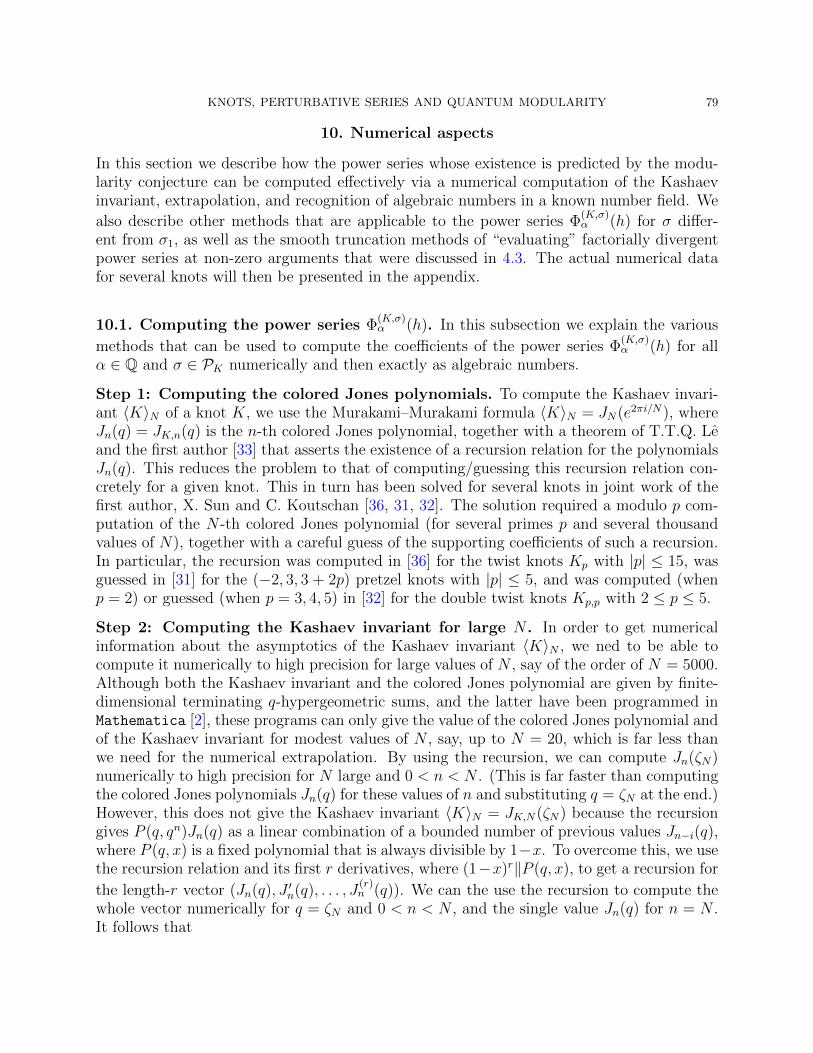
KNOTS, PERTURBATIVE SERIES AND QUANTUM MODULARITY 79
10. Numerical aspects
In this section we describe how the power series whose existence is predicted by the modu-larity conjecture can be computed effectively via a numerical computation of the Kashaevinvariant, extrapolation, and recognition of algebraic numbers in a known number field. We
also describe other methods that are applicable to the power series Φ(K,σ)α (h) for σ differ-
ent from σ1, as well as the smooth truncation methods of “evaluating” factorially divergentpower series at non-zero arguments that were discussed in 4.3. The actual numerical datafor several knots will then be presented in the appendix.
10.1. Computing the power series Φ(K,σ)α (h). In this subsection we explain the various
methods that can be used to compute the coefficients of the power series Φ(K,σ)α (h) for all
α ∈ Q and σ ∈ PK numerically and then exactly as algebraic numbers.
Step 1: Computing the colored Jones polynomials. To compute the Kashaev invari-ant 〈K〉N of a knot K, we use the Murakami–Murakami formula 〈K〉N = JN(e2πi/N), whereJn(q) = JK,n(q) is the n-th colored Jones polynomial, together with a theorem of T.T.Q. Leand the first author [33] that asserts the existence of a recursion relation for the polynomialsJn(q). This reduces the problem to that of computing/guessing this recursion relation con-cretely for a given knot. This in turn has been solved for several knots in joint work of thefirst author, X. Sun and C. Koutschan [36, 31, 32]. The solution required a modulo p com-putation of the N -th colored Jones polynomial (for several primes p and several thousandvalues of N), together with a careful guess of the supporting coefficients of such a recursion.In particular, the recursion was computed in [36] for the twist knots Kp with |p| ≤ 15, wasguessed in [31] for the (−2, 3, 3 + 2p) pretzel knots with |p| ≤ 5, and was computed (whenp = 2) or guessed (when p = 3, 4, 5) in [32] for the double twist knots Kp,p with 2 ≤ p ≤ 5.
Step 2: Computing the Kashaev invariant for large N . In order to get numericalinformation about the asymptotics of the Kashaev invariant 〈K〉N , we ned to be able tocompute it numerically to high precision for large values of N , say of the order of N = 5000.Although both the Kashaev invariant and the colored Jones polynomial are given by finite-dimensional terminating q-hypergeometric sums, and the latter have been programmed inMathematica [2], these programs can only give the value of the colored Jones polynomial andof the Kashaev invariant for modest values of N , say, up to N = 20, which is far less thanwe need for the numerical extrapolation. By using the recursion, we can compute Jn(ζN)numerically to high precision for N large and 0 < n < N . (This is far faster than computingthe colored Jones polynomials Jn(q) for these values of n and substituting q = ζN at the end.)However, this does not give the Kashaev invariant 〈K〉N = JK,N(ζN) because the recursiongives P (q, qn)Jn(q) as a linear combination of a bounded number of previous values Jn−i(q),where P (q, x) is a fixed polynomial that is always divisible by 1−x. To overcome this, we usethe recursion relation and its first r derivatives, where (1−x)r‖P (q, x), to get a recursion for
the length-r vector (Jn(q), J ′n(q), . . . , J(r)n (q)). We can the use the recursion to compute the
whole vector numerically for q = ζN and 0 < n < N , and the single value Jn(q) for n = N .It follows that
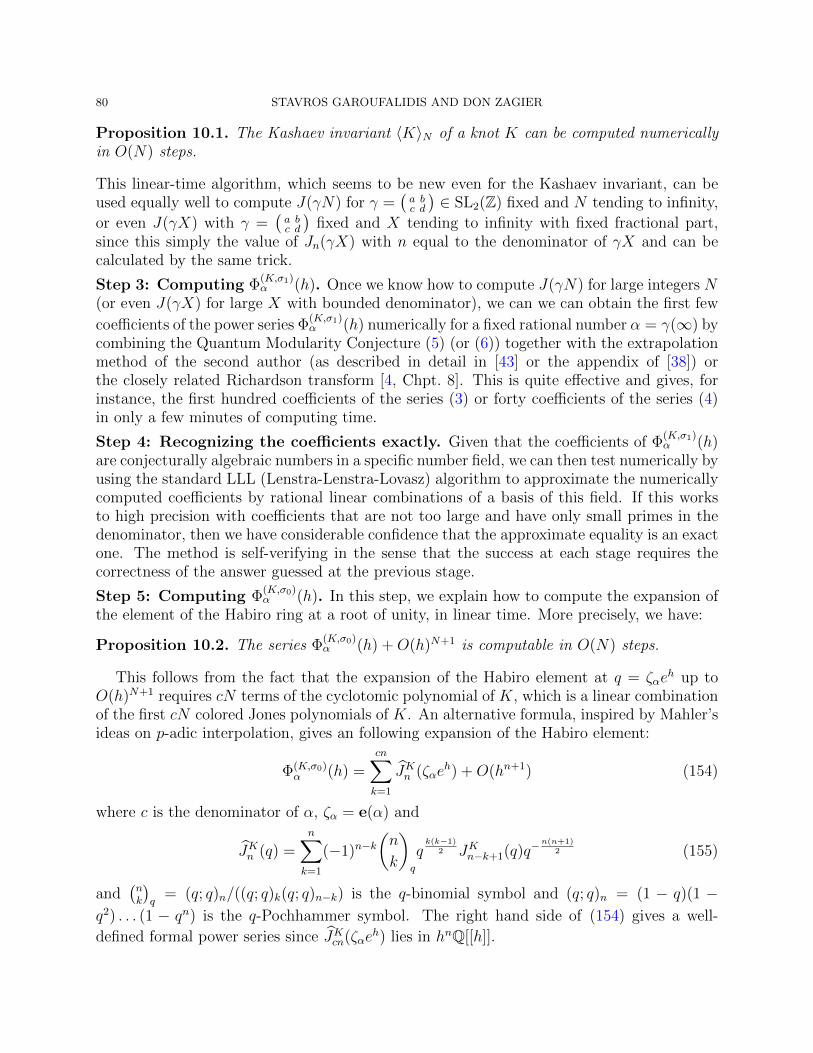
80 STAVROS GAROUFALIDIS AND DON ZAGIER
Proposition 10.1. The Kashaev invariant 〈K〉N of a knot K can be computed numericallyin O(N) steps.
This linear-time algorithm, which seems to be new even for the Kashaev invariant, can beused equally well to compute J(γN) for γ =
(a bc d
)∈ SL2(Z) fixed and N tending to infinity,
or even J(γX) with γ =(a bc d
)fixed and X tending to infinity with fixed fractional part,
since this simply the value of Jn(γX) with n equal to the denominator of γX and can becalculated by the same trick.
Step 3: Computing Φ(K,σ1)α (h). Once we know how to compute J(γN) for large integers N
(or even J(γX) for large X with bounded denominator), we can we can obtain the first few
coefficients of the power series Φ(K,σ1)α (h) numerically for a fixed rational number α = γ(∞) by
combining the Quantum Modularity Conjecture (5) (or (6)) together with the extrapolationmethod of the second author (as described in detail in [43] or the appendix of [38]) orthe closely related Richardson transform [4, Chpt. 8]. This is quite effective and gives, forinstance, the first hundred coefficients of the series (3) or forty coefficients of the series (4)in only a few minutes of computing time.
Step 4: Recognizing the coefficients exactly. Given that the coefficients of Φ(K,σ1)α (h)
are conjecturally algebraic numbers in a specific number field, we can then test numerically byusing the standard LLL (Lenstra-Lenstra-Lovasz) algorithm to approximate the numericallycomputed coefficients by rational linear combinations of a basis of this field. If this worksto high precision with coefficients that are not too large and have only small primes in thedenominator, then we have considerable confidence that the approximate equality is an exactone. The method is self-verifying in the sense that the success at each stage requires thecorrectness of the answer guessed at the previous stage.
Step 5: Computing Φ(K,σ0)α (h). In this step, we explain how to compute the expansion of
the element of the Habiro ring at a root of unity, in linear time. More precisely, we have:
Proposition 10.2. The series Φ(K,σ0)α (h) +O(h)N+1 is computable in O(N) steps.
This follows from the fact that the expansion of the Habiro element at q = ζαeh up to
O(h)N+1 requires cN terms of the cyclotomic polynomial of K, which is a linear combinationof the first cN colored Jones polynomials of K. An alternative formula, inspired by Mahler’sideas on p-adic interpolation, gives an following expansion of the Habiro element:
Φ(K,σ0)α (h) =
cn∑k=1
JKn (ζαeh) +O(hn+1) (154)
where c is the denominator of α, ζα = e(α) and
JKn (q) =n∑k=1
(−1)n−k(n
k
)q
qk(k−1)
2 JKn−k+1(q)q−n(n+1)
2 (155)
and(nk
)q
= (q; q)n/((q; q)k(q; q)n−k) is the q-binomial symbol and (q; q)n = (1 − q)(1 −q2) . . . (1 − qn) is the q-Pochhammer symbol. The right hand side of (154) gives a well-
defined formal power series since JKcn(ζαeh) lies in hnQ[[h]].
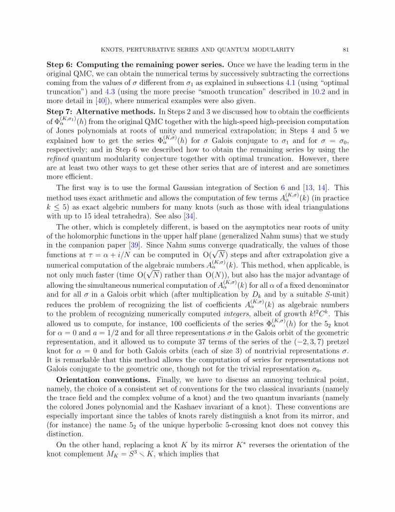
KNOTS, PERTURBATIVE SERIES AND QUANTUM MODULARITY 81
Step 6: Computing the remaining power series. Once we have the leading term in theoriginal QMC, we can obtain the numerical terms by successively subtracting the correctionscoming from the values of σ different from σ1 as explained in subsections 4.1 (using “optimaltruncation”) and 4.3 (using the more precise “smooth truncation” described in 10.2 and inmore detail in [40]), where numerical examples were also given.
Step 7: Alternative methods. In Steps 2 and 3 we discussed how to obtain the coefficients
of Φ(K,σ1)α (h) from the original QMC together with the high-speed high-precision computation
of Jones polynomials at roots of unity and numerical extrapolation; in Steps 4 and 5 we
explained how to get the series Φ(K,σ)α (h) for σ Galois conjugate to σ1 and for σ = σ0,
respectively; and in Step 6 we described how to obtain the remaining series by using therefined quantum modularity conjecture together with optimal truncation. However, thereare at least two other ways to get these other series that are of interest and are sometimesmore efficient.
The first way is to use the formal Gaussian integration of Section 6 and [13, 14]. This
method uses exact arithmetic and allows the computation of few terms A(K,σ)α (k) (in practice
k ≤ 5) as exact algebric numbers for many knots (such as those with ideal triangulationswith up to 15 ideal tetrahedra). See also [34].
The other, which is completely different, is based on the asymptotics near roots of unityof the holomorphic functions in the upper half plane (generalized Nahm sums) that we studyin the companion paper [39]. Since Nahm sums converge quadratically, the values of those
functions at τ = α + i/N can be computed in O(√N) steps and after extrapolation give a
numerical computation of the algebraic numbers A(K,σ)α (k). This method, when applicable, is
not only much faster (time O(√N) rather than O(N)), but also has the major advantage of
allowing the simultaneous numerical computation of A(K,σ)α (k) for all α of a fixed denominator
and for all σ in a Galois orbit which (after multiplication by Dk and by a suitable S-unit)
reduces the problem of recognizing the list of coefficients A(K,σ)α (k) as algebraic numbers
to the problem of recognizing numerically computed integers, albeit of growth k!2Ck. This
allowed us to compute, for instance, 100 coefficients of the series Φ(K,σ)α (h) for the 52 knot
for α = 0 and a = 1/2 and for all three representations σ in the Galois orbit of the geometricrepresentation, and it allowed us to compute 37 terms of the series of the (−2, 3, 7) pretzelknot for α = 0 and for both Galois orbits (each of size 3) of nontrivial representations σ.It is remarkable that this method allows the computation of series for representations notGalois conjugate to the geometric one, though not for the trivial representation σ0.
Orientation conventions. Finally, we have to discuss an annoying technical point,namely, the choice of a consistent set of conventions for the two classical invariants (namelythe trace field and the complex volume of a knot) and the two quantum invariants (namelythe colored Jones polynomial and the Kashaev invariant of a knot). These conventions areespecially important since the tables of knots rarely distinguish a knot from its mirror, and(for instance) the name 52 of the unique hyperbolic 5-crossing knot does not convey thisdistinction.
On the other hand, replacing a knot K by its mirror K∗ reverses the orientation of theknot complement MK = S3 rK, which implies that
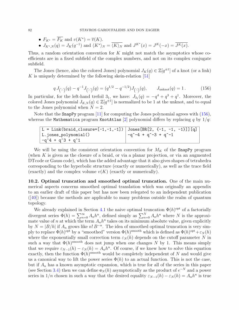
82 STAVROS GAROUFALIDIS AND DON ZAGIER
• FK∗ = FK and v(K∗) = v(K).
• JK∗,N(q) = JK(q−1) and 〈K∗〉N = 〈K〉N and JK∗(x) = JK(−x) = JK(x).
Thus, a random orientation convention for K might not match the asymptotics whose co-efficients are in a fixed subfield of the complex numbers, and not on its complex conjugatesubfield.
The Jones (hence, also the colored Jones) polynomial JK(q) ∈ Z[q±1] of a knot (or a link)K is uniquely determined by the following skein-relation [51]
q J( )(q)− q−1J( )(q) = (q1/2 − q−1/2)J( )(q), Junknot(q) = 1 . (156)
In particular, for the left-hand trefoil 31, we have: J31(q) = −q4 + q3 + q1. Moreover, thecolored Jones polynomial JK,N(q) ∈ Z[q±1] is normalized to be 1 at the unknot, and to equalto the Jones polynomial when N = 2.
Note that the SnapPy program [11] for computing the Jones polynomial agrees with (156),whereas the Mathematica program KnotAtlas [2] polynomial differs by replacing q by 1/q:
L = Link(braid_closure=[-1,-1,-1]) Jones[BR[2, {-1, -1, -1}]][q]
L.jones_polynomial() -q^-4 + q^-3 + q^-1
-q^4 + q^3 + q^1
We will be using the consistent orientation convention for MK of the SnapPy program(when K is given as the closure of a braid, or via a planar projection, or via an augmentedDTcode or Gauss code), which has the added advantage that it also gives shapes of tetrahedracorresponding to the hyperbolic structure (exactly or numerically), as well as the trace field(exactly) and the complex volume v(K) (exactly or numerically).
10.2. Optimal truncation and smoothed optimal truncation. One of the main nu-merical aspects concerns smoothed optimal translation which was originally an appendixto an earlier draft of this paper but has now been relegated to an independent publication([40]) because the methods are applicable to many problems outside the realm of quantumtopology.
We already explained in Section 4.1 the naive optimal truncation Φ(h)opt of a factorially
divergent series Φ(h) =∑∞
n=0Anhn, defined simply as
∑Nn=0Anh
n where N is the approxi-mate value of n at which the term Anh
n takes on its minimum absolute value, given explicitlyby N = |B/h| if An grows like n!B−n. The idea of smoothed optimal truncation is very sim-ply to replace Φ(h)opt by a “smoothed” version Φ(h)smooth which is defined as Φ(h)opt +εN(h)where the exponentially small correction term εN(h) depends on the cutoff parameter N insuch a way that Φ(h)smooth does not jump when one changes N by 1. This means simplythat we require εN−1(h)− εN(h) = Anh
n. Of course, if we knew how to solve this equationexactly, then the function Φ(h)smooth would be completely independent of N and would giveus a canonical way to lift the power series Φ(h) to an actual function. This is not the case,but if An has a known asymptotic expansion, which is true for all of the series in this paper(see Section 3.4) then we can define eN(h) asymptotically as the product of e−N and a powerseries in 1/n chosen in such a way that the desired equality εN−1(h)− εN(h) = Anh
n is true
KNOTS, PERTURBATIVE SERIES AND QUANTUM MODULARITY 83
asymptotically to all orders in 1/n. The details of how to do this if An has the asymptoticform B−n
∑∞`=0 c` Γ(n + κ − `) for some real number κ and some numerical coefficients c`
(as in equations (36), (37) or (38)) are given in [40] and will not be repeated here. The onlything that is of importance to us here is that the result of the smoothing gives an evaluationof Φ(h) that is independent of all choices (and hence gives a predicted “right” definition ofthe corresponding function) up to an error that is exponentially small with a better exponentthan that given by naive optimal truncation. Specifically, the new error is e−N (1 + |C|)−Nrather than simply e−N as before if, as is always the case for us, the coefficients c` themselvesgrow factorially like `!C−`. Examples of this dramatic numerical improvement were given inSection 4.3, where in one case the error in evaluating a series Φ(h) was of the order of 10−29
using naive optimal truncation but of the order of 10−56 using smoothed optimal truncation.
84 STAVROS GAROUFALIDIS AND DON ZAGIER
Appendix: Numerical data for five sample knots
In this section we present numerical data that support the quantum modularity conjecturefor a choice of knots. Initially, we hoped that pairs of geometrically similar knots (that haveidentical trace fields and equal elements in the Bloch group, modulo torsion—henceforth
called “sisters”) might have identical or nearly identical series Φ(K,σ1)α . With this in mind,
and having already performed the computations for the 41 knot, we were led to consider itssister, the m003 census manifold. The latter is not a knot complement (it is the complementof a knot in a lens space), but its 5-fold cyclic cover is the complement of the (twisted) 5-chain link, with a computable Kashaev invariant, to be compared with the 5-th power of the
Kashaev invariant of the 41 knot. No relation between the series Φ(K,σ1)α was found for this
pair, but the units ε(K)α did match (up to roots of unity). We then tried the 52 knot, whose
sister is the (−2, 3, 7) pretzel knot. Here again the series Φ(K,σ1)α were different, but the units
ε(K)α matched. The final example of the 61 knot was chosen because its Bloch group hasrank 2 and its SL2(C)-character variety is more complicated, making the verification of theQMC, the Galois invariance property (143) and the match with the unit of [9] more subtle,but again all three were verified numerically. For this knot we did not make any “sister”computations.
Recall the coefficients A(K,σ)α (k) of the power series Φ
(K,σ)α (h) are algebraic numbers. In
this section, we present the numerically obtained data for A(K,σ)α (k) written in the form
A(K,σ)α (k) = C(K,σ)
α A(K,σ)α (k) , (157)
where C(K,σ)α = µσ,α · (εσ,α)
1c · δ−
12
σ is given in (144). Note however that C(K,σ)α and A
(K,σ)α (k)
are not canonically defined numbers, only their product is. (Since we are focusing on thegeometric representation σ1, and we are fixing the knot K, we omit the superscript (K, σ)from the notation in the right hand side of the above equation.) We will further specify
a choice of an algebraic number λc such that λkc Dk Aα(k) ∈ OF (ζα) is an algebraic integer,where c is the denominator of α, F is the trace field of the knot and Dn is the universaldenominator (142). Using a basis of free abelian groups OF (ζα) we can represent the abovealgebraic integers by lists of integer numbers.
The figure eight knot. In this section we discuss the numerical aspects of the quantummodularity conjecture for the simplest hyperbolic 41 knot, for which we currently know howto prove the modularity conjecture. (The proof was presented in Section 8.) Needless tosay, the numerically obtained results agree with the exact computation of the expansion co-efficients given in Section 8. Some information about the numerical aspects of the Kashaevinvariant of the 41 knot were already presented in the introduction, but we give some ad-ditional data (e.g., for the expansion near seventh roots of unity), since this is the mostaccessible knot numerically and also to illustrate the formulas occuring in the proof.
Since the knot is fixed in this section, and so is the geometric representation σ1, we willsuppress them from the notation. As mentioned in Section 1, the trace field of the 41 knotis Q(
√−3) and the torsion is δ =
√−3. Some terms of the series Φα(h) when c = 1 or
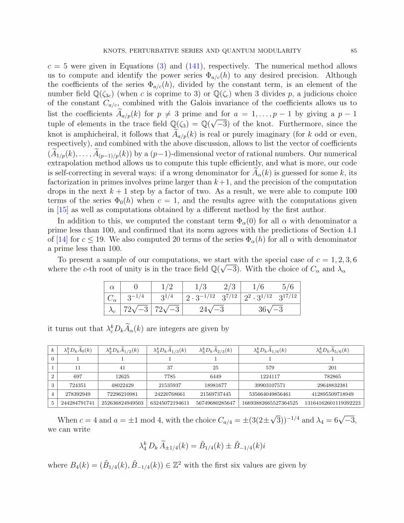
KNOTS, PERTURBATIVE SERIES AND QUANTUM MODULARITY 85
c = 5 were given in Equations (3) and (141), respectively. The numerical method allowsus to compute and identify the power series Φa/c(h) to any desired precision. Althoughthe coefficients of the series Φa/c(h), divided by the constant term, is an element of thenumber field Q(ζ3c) (when c is coprime to 3) or Q(ζc) when 3 divides p, a judicious choiceof the constant Ca/c, combined with the Galois invariance of the coefficients allows us to
list the coefficients Aa/p(k) for p 6= 3 prime and for a = 1, . . . , p − 1 by giving a p − 1
tuple of elements in the trace field Q(ζ3) = Q(√−3) of the knot. Furthermore, since the
knot is amphicheiral, it follows that Aa/p(k) is real or purely imaginary (for k odd or even,respectively), and combined with the above discussion, allows to list the vector of coefficients
(A1/p(k), . . . , A(p−1)/p(k)) by a (p−1)-dimensional vector of rational numbers. Our numericalextrapolation method allows us to compute this tuple efficiently, and what is more, our code
is self-correcting in several ways: if a wrong denominator for Aα(k) is guessed for some k, itsfactorization in primes involves prime larger than k+1, and the precision of the computationdrops in the next k + 1 step by a factor of two. As a result, we were able to compute 100terms of the series Φ0(h) when c = 1, and the results agree with the computations givenin [15] as well as computations obtained by a different method by the first author.
In addition to this, we computed the constant term Φα(0) for all α with denominator aprime less than 100, and confirmed that its norm agrees with the predictions of Section 4.1of [14] for c ≤ 19. We also computed 20 terms of the series Φα(h) for all α with denominatora prime less than 100.
To present a sample of our computations, we start with the special case of c = 1, 2, 3, 6where the c-th root of unity is in the trace field Q(
√−3). With the choice of Cα and λα
α 0 1/2 1/3 2/3 1/6 5/6
Cα 3−1/4 31/4 2 · 3−1/12 37/12 22 · 31/12 317/12
λc 72√−3 72
√−3 24
√−3 36
√−3
it turns out that λkcDkAα(k) are integers are given by
k λk1DkA0(k) λk2DkA1/2(k) λk3DkA1/3(k) λk3DkA2/3(k) λk6DkA1/6(k) λk6DkA5/6(k)
0 1 1 1 1 1 1
1 11 41 37 25 579 201
2 697 12625 7785 6449 1224117 782865
3 724351 48022429 21535937 18981677 39903107571 29648832381
4 278392949 72296210981 24220768661 21569737445 535664049856461 412895509718949
5 244284791741 252636824949503 63245072194611 56749680285647 16693882665527364525 13164162601119392223
When c = 4 and a = ±1 mod 4, with the choice Ca/4 = ±(3(2±√
3))−1/4 and λ4 = 6√−3,
we can write
λk4 Dk A±1/4(k) = B1/4(k)± B−1/4(k)i
where B4(k) = (B1/4(k), B−1/4(k)) ∈ Z2 with the first six values are given by
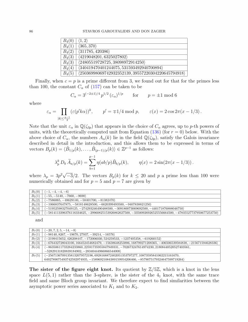
86 STAVROS GAROUFALIDIS AND DON ZAGIER
B4(0) 〈1, 2〉B4(1) 〈365, 370〉B4(2) 〈311785, 420386〉B4(3) 〈4219048201, 6325027802〉B4(3) 〈24805519728725, 38098972914250〉B4(4) 〈340419470401244075, 531593492940700894〉B4(5) 〈25036998069742932352139, 39557220304220645794918〉
Finally, when c = p is a prime different from 3, we found out for that for the primes lessthan 100, the constant Cα of (157) can be taken to be
Cα = 3(−2±1)/4 p1/2 (εα)1/p for p = ±1 mod 6
where
εα =∏|k|≤ p−1
2
(ε(p′kα))k, p′ = ∓1/4 mod p, ε(x) = 2 cos 2π(x− 1/3) .
Note that the unit εα in Q(ζ3p) that appears in the choice of Cα agrees, up to p-th powers ofunits, with the theoretically computed unit from Equation (136) (for r = 0) below. With theabove choice of Cα, the numbers Aα(k) lie in the field Q(ζ3p), satisfy the Galois invariancedescribed in detail in the introduction, and this allows them to be expressed in terms ofvectors Bp(k) = 〈B1/p(k), . . . , B(p−1)/p(k)〉 ∈ Zp−1 as follows:
λkpDk Aa/p(k) =
p−1∑b=1
η(ab/p)Bb/p(k), η(x) = 2 sin(2π(x− 1/3)) .
where λp = 3p2√−3/2. The vectors Bp(k) for k ≤ 20 and p a prime less than 100 were
numerically obtained and for p = 5 and p = 7 are given by
B5(0) 〈−1,−4,−4,−6〉B5(1) 〈−55,−5140,−7660,−9690〉B5(2) 〈−7586065,−48629140,−58401700,−81382470〉B5(3) 〈−1066837647875,−5818148628500,−6620399493500,−9407838821250〉B5(4) 〈−51952598327049125,−274293246490488500,−309180073069692500,−440171876888046750〉B5(5) 〈−5814113396376116334625,−29960825153926862627500,−33500926926525556664500,−47835527737950677253750〉
and
B7(0) 〈−20, 7, 2, 5,−14,−8〉B7(1) 〈−98140, 8267,−19670, 27937,−39214,−16576〉B7(2) 〈−2199415652, 426208447,−172006030, 524259533,−1237405358,−619260152〉B7(3) 〈−676432728043100, 166452454682479,−15638648253886, 168799271208365,−406506539584838,−215671594628336〉B7(4) 〈−86350611733284233860, 22591735955847949331,−702673247614974230, 21808440520527403561,
−52829131820839184902,−28340444966866544008〉B7(5) 〈−25671367091358132079572196, 6928168872402051353797277, 10873595841062215161670,
6492789075493742592974935,−15896921084389159954206466,−8579075179324647599719264〉
The sister of the figure eight knot. Its quotient by Z/5Z, which is a knot in the lensspace L(5, 1) rather than the 3-sphere, is the sister of the 41 knot, with the same tracefield and same Bloch group invariant. We therefore expect to find similarities between theasymptotic power series associated to K1 and to K2.
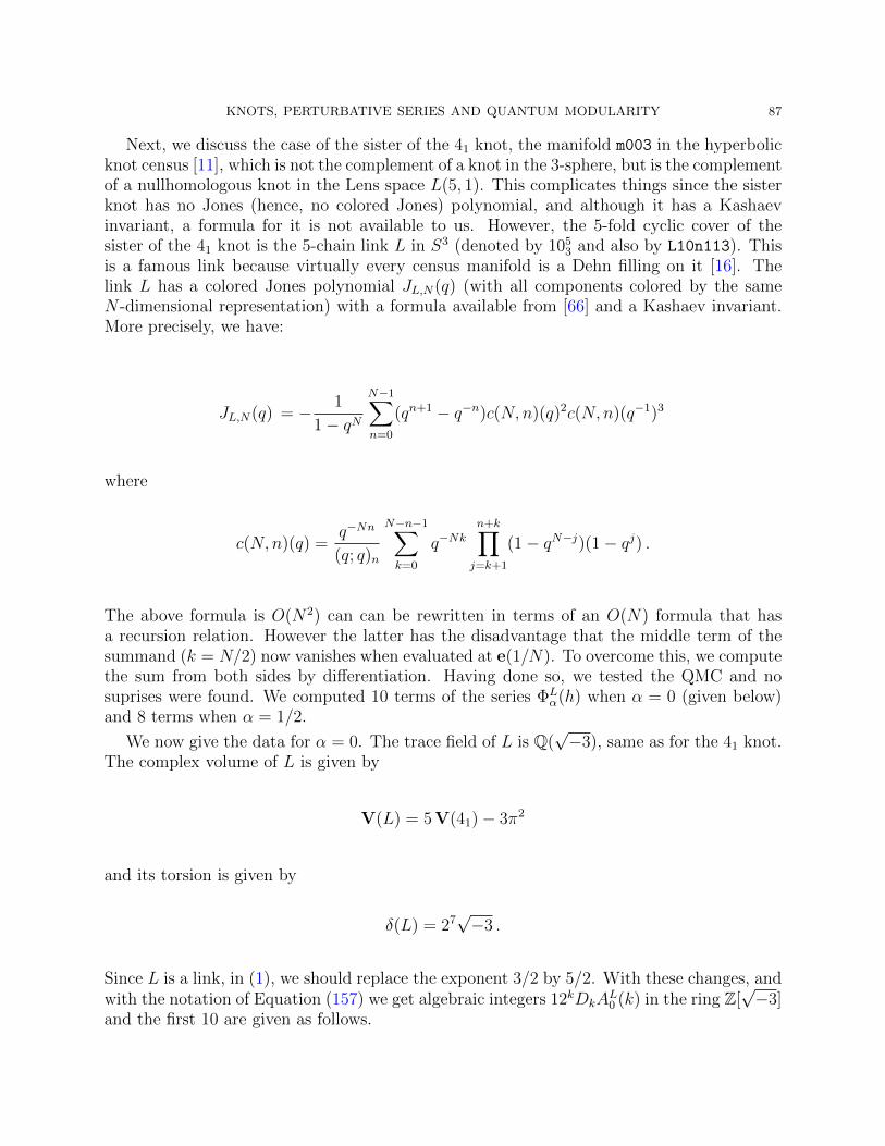
KNOTS, PERTURBATIVE SERIES AND QUANTUM MODULARITY 87
Next, we discuss the case of the sister of the 41 knot, the manifold m003 in the hyperbolicknot census [11], which is not the complement of a knot in the 3-sphere, but is the complementof a nullhomologous knot in the Lens space L(5, 1). This complicates things since the sisterknot has no Jones (hence, no colored Jones) polynomial, and although it has a Kashaevinvariant, a formula for it is not available to us. However, the 5-fold cyclic cover of thesister of the 41 knot is the 5-chain link L in S3 (denoted by 105
3 and also by L10n113). Thisis a famous link because virtually every census manifold is a Dehn filling on it [16]. Thelink L has a colored Jones polynomial JL,N(q) (with all components colored by the sameN -dimensional representation) with a formula available from [66] and a Kashaev invariant.More precisely, we have:
JL,N(q) = − 1
1− qNN−1∑n=0
(qn+1 − q−n)c(N, n)(q)2c(N, n)(q−1)3
where
c(N, n)(q) =q−Nn
(q; q)n
N−n−1∑k=0
q−Nkn+k∏j=k+1
(1− qN−j)(1− qj) .
The above formula is O(N2) can can be rewritten in terms of an O(N) formula that hasa recursion relation. However the latter has the disadvantage that the middle term of thesummand (k = N/2) now vanishes when evaluated at e(1/N). To overcome this, we computethe sum from both sides by differentiation. Having done so, we tested the QMC and nosuprises were found. We computed 10 terms of the series ΦL
α(h) when α = 0 (given below)and 8 terms when α = 1/2.
We now give the data for α = 0. The trace field of L is Q(√−3), same as for the 41 knot.
The complex volume of L is given by
V(L) = 5 V(41)− 3π2
and its torsion is given by
δ(L) = 27√−3 .
Since L is a link, in (1), we should replace the exponent 3/2 by 5/2. With these changes, andwith the notation of Equation (157) we get algebraic integers 12kDkA
L0 (k) in the ring Z[
√−3]
and the first 10 are given as follows.
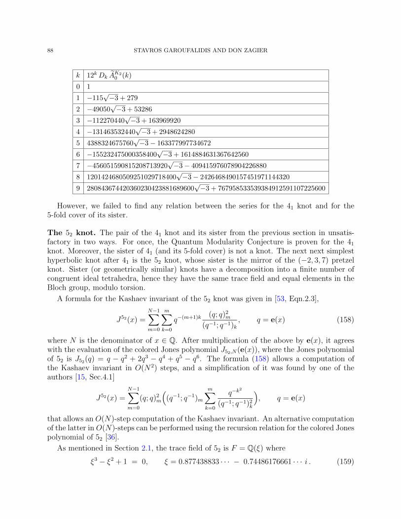
88 STAVROS GAROUFALIDIS AND DON ZAGIER
k 12kDk AK20 (k)
0 1
1 −115√−3 + 279
2 −49050√−3 + 53286
3 −112270440√−3 + 163969920
4 −131463532440√−3 + 2948624280
5 4388324675760√−3− 163377997734672
6 −155232475000358400√−3 + 1614884631367642560
7 −456051590815208713920√−3− 409415976078904226880
8 1201424680509251029718400√−3− 2426468490157451971144320
9 280843674420360230423881689600√−3 + 767958533539384912591107225600
However, we failed to find any relation between the series for the 41 knot and for the5-fold cover of its sister.
The 52 knot. The pair of the 41 knot and its sister from the previous section in unsatis-factory in two ways. For once, the Quantum Modularity Conjecture is proven for the 41
knot. Moreover, the sister of 41 (and its 5-fold cover) is not a knot. The next next simplesthyperbolic knot after 41 is the 52 knot, whose sister is the mirror of the (−2, 3, 7) pretzelknot. Sister (or geometrically similar) knots have a decomposition into a finite number ofcongruent ideal tetrahedra, hence they have the same trace field and equal elements in theBloch group, modulo torsion.
A formula for the Kashaev invariant of the 52 knot was given in [53, Eqn.2.3],
J52(x) =N−1∑m=0
m∑k=0
q−(m+1)k (q; q)2m
(q−1; q−1)k, q = e(x) (158)
where N is the denominator of x ∈ Q. After multiplication of the above by e(x), it agreeswith the evaluation of the colored Jones polynomial J52,N(e(x)), where the Jones polynomialof 52 is J52(q) = q − q2 + 2q3 − q4 + q5 − q6. The formula (158) allows a computation ofthe Kashaev invariant in O(N2) steps, and a simplification of it was found by one of theauthors [15, Sec.4.1]
J52(x) =N−1∑m=0
(q; q)2m
((q−1; q−1)m
m∑k=0
q−k2
(q−1; q−1)2k
), q = e(x)
that allows an O(N)-step computation of the Kashaev invariant. An alternative computationof the latter in O(N)-steps can be performed using the recursion relation for the colored Jonespolynomial of 52 [36].
As mentioned in Section 2.1, the trace field of 52 is F = Q(ξ) where
ξ3 − ξ2 + 1 = 0, ξ = 0.877438833 · · · − 0.74486176661 · · · i . (159)
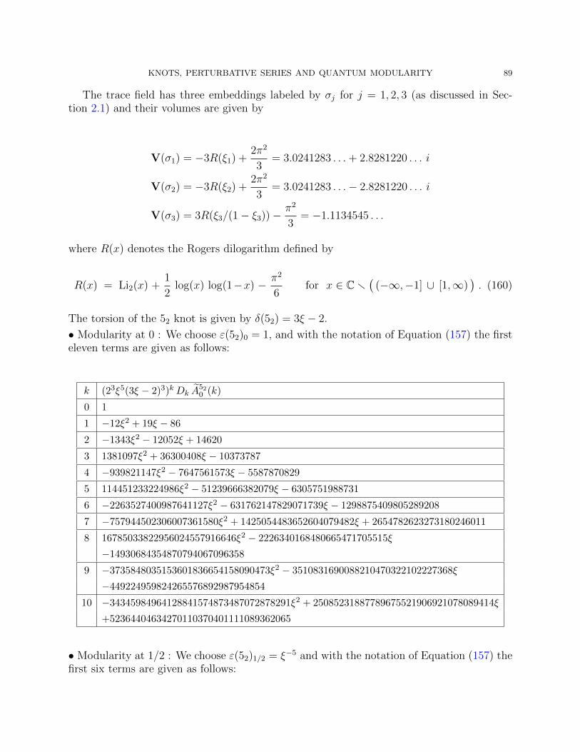
KNOTS, PERTURBATIVE SERIES AND QUANTUM MODULARITY 89
The trace field has three embeddings labeled by σj for j = 1, 2, 3 (as discussed in Sec-tion 2.1) and their volumes are given by
V(σ1) = −3R(ξ1) +2π2
3= 3.0241283 . . .+ 2.8281220 . . . i
V(σ2) = −3R(ξ2) +2π2
3= 3.0241283 . . .− 2.8281220 . . . i
V(σ3) = 3R(ξ3/(1− ξ3))− π2
3= −1.1134545 . . .
where R(x) denotes the Rogers dilogarithm defined by
R(x) = Li2(x) +1
2log(x) log(1−x) − π2
6for x ∈ Cr
((−∞,−1] ∪ [1,∞)
). (160)
The torsion of the 52 knot is given by δ(52) = 3ξ − 2.
• Modularity at 0 : We choose ε(52)0 = 1, and with the notation of Equation (157) the firsteleven terms are given as follows:
k (23ξ5(3ξ − 2)3)kDk A520 (k)
0 1
1 −12ξ2 + 19ξ − 86
2 −1343ξ2 − 12052ξ + 14620
3 1381097ξ2 + 36300408ξ − 10373787
4 −939821147ξ2 − 7647561573ξ − 5587870829
5 114451233224986ξ2 − 51239666382079ξ − 6305751988731
6 −2263527400987641127ξ2 − 631762147829071739ξ − 1298875409805289208
7 −757944502306007361580ξ2 + 1425054483652604079482ξ + 2654782623273180246011
8 16785033822956024557916646ξ2 − 2226340168480665471705515ξ
−14930684354870794067096358
9 −3735848035153601836654158090473ξ2 − 3510831690088210470322102227368ξ
−449224959824265576892987954854
10 −34345984964128841574873487072878291ξ2 + 25085231887789675521906921078089414ξ
+52364404634270110370401111089362065
• Modularity at 1/2 : We choose ε(52)1/2 = ξ−5 and with the notation of Equation (157) thefirst six terms are given as follows:
90 STAVROS GAROUFALIDIS AND DON ZAGIER
k (2 ξ5(3ξ − 2)3)kDk A521/2(k)
0 ξ + 2
1 307ξ2 − 138ξ − 628
2 −573109ξ2 − 168712ξ + 457975
3 2096955561ξ2 + 5077310601ξ + 1165885531
4 6470888990010ξ2 − 5414463743327ξ − 10380246225743
5 289484322041800655ξ2 − 138373378538474483ξ − 156775910252412286
• Modularity at 1/3 : Here, the constant term Φ521/3(0) was numerically computed to high
precision
Φ521/3(0) = −1.3478490468923913068 · · · − 1.5706460265356353326 . . . i
but was not initially recognized. To identify it, we used the formula (158) for the Kashaevinvariant and performed a theoretical computation analogous to the constants S(α) andE0(α) (given in (136) and (140)) of the 41 knot which produced the primes
p7 = (ξ2 − 1)ζ6 − ξ + 1, p43 = 2ξ2 − ξ − ζ6
of norm 7 and 43 respectively in the number field F3 = Q(ξ, ζ3). Note that the same primesappear in [14, Sec.6.2]. In addition, the above constant involves δ(52)−1/2 and a numberwhose third power is in F3. After some experimentation, we concluded that
Φ521/3(0) = e(1/36)
1√3ξ − 2
p27 p43 .
It follows that a representative of the unit at α = 1/3 is given by
ε(52)1/3 = e(1/12) . (161)
It was a bit of a surprise to find that the unit is torsion although the Bloch group of F61 hasrank 1–on the other hand 3 (as well as 2 and a few other primes) are exceptional ones in thework [9].
Once the constant term was recognized, it turnt out that we needed to separate one factorof p7 in the constant term Φ52
1/3(0) from the remaining terms, in order to avoid spurious
denominators. With the choice of C1/3 = e(1/36)(3ξ− 2)−12p7 p43 and the notation of (157),
the first seven terms were found
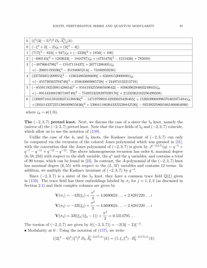
KNOTS, PERTURBATIVE SERIES AND QUANTUM MODULARITY 91
k (ξ5(3ξ − 2)3)kDk A521/3(k)
0 (−ξ2 + 2ξ − 2)ζ6 + (2ξ2 − 4ξ)
1 (717ξ2 − 822ξ + 947)ζ6 + (−2226ξ2 + 1856ξ + 106)
2 (−680145ξ2 + 1283633ξ − 1844797)ζ6 + (4731470ξ2 − 1215426ξ + 785050)
3 (−4879664798ξ2 − 15547118437ξ + 26771206405)ζ6
+(−20691193336ξ2 − 35194065214ξ − 73160959238)
4 (237593851209955ξ2 − 123624865686699ξ + 65688152000880)ζ6
+(−455730563794746ξ2 + 258640669065738ξ + 244974132213716)
5 (−8559119253981428654ξ2 + 9164193255880569642ξ − 8506396294603249043)ζ6
+(−8914434881967188748ξ2 − 7549553228397039176ξ + 21232362162256499338)
6 (1206971041591026374138836ξ2 − 1471979903142920023426465ξ + 1526039068996370402375484)ζ6
+(2034143372251380409655636ξ2 + 5390411863643322238842526ξ − 935392258601663466664696)
where ζ6 = e(1/6).
The (−2, 3, 7) pretzel knot. Next, we discuss the case of a sister the 52 knot, namely the(mirror of) the (−2, 3, 7) pretzel knot. Note that the trace fields of 52 and (−2, 3, 7) coincide,which allow us to use the notation of (159).
Unlike the case of the 41 and 52 knots, the Kashaev invariant of (−2, 3, 7) can onlybe computed via the recursion of the colored Jones polynomial which was guessed in [31],with the convention that the Jones polynomial of (−2, 3, 7) is given by J (−2,3,7)(q) = q−5 +q−7 − q−11 + q−12 − q−13. The above inhomogeneous recursion has order 6, maximal degree(6, 58, 233) with respect to the shift variable, the qn and the q variables, and contains a totalof 90 terms, which can be found in [23]. In contrast, the A-polynomial of the (−2, 3, 7) knothas maximal degree (6, 55) with respect to the (L,M) variables and contains 12 terms. Inaddition, we multiply the Kashaev invariant of (−2, 3, 7) by q−4.
Since (−2, 3, 7) is a sister of the 52 knot, they have a common trace field Q(ξ) givenin (159). The trace field has three embeddings labeled by σj for j = 1, 2, 3 (as discussed inSection 2.1) and their complex volumes are given by
V(σ1) = −3R(ξ1) +π2
3= 4.6690624 . . .+ 2.8281220 . . . i
V(σ2) = −3R(ξ2) +π2
3= 4.6690624 . . .− 2.8281220 . . . i
V(σ3) = 3R(ξ3/(ξ3 − 1)) +π2
3= 0.5314795 . . .
The torsion of (−2, 3, 7) are given by δ((−2, 3, 7)) = −2(3ξ − 2)ξ−2.
• Modularity at 0 : Using the notation of (157), we write
((2ξ2 − 6)3/ξ5)kDk A(−2,3,7),σ10 (k) = (1, ξ, ξ2) ·B(−2,3,7),σ1
0 (k)
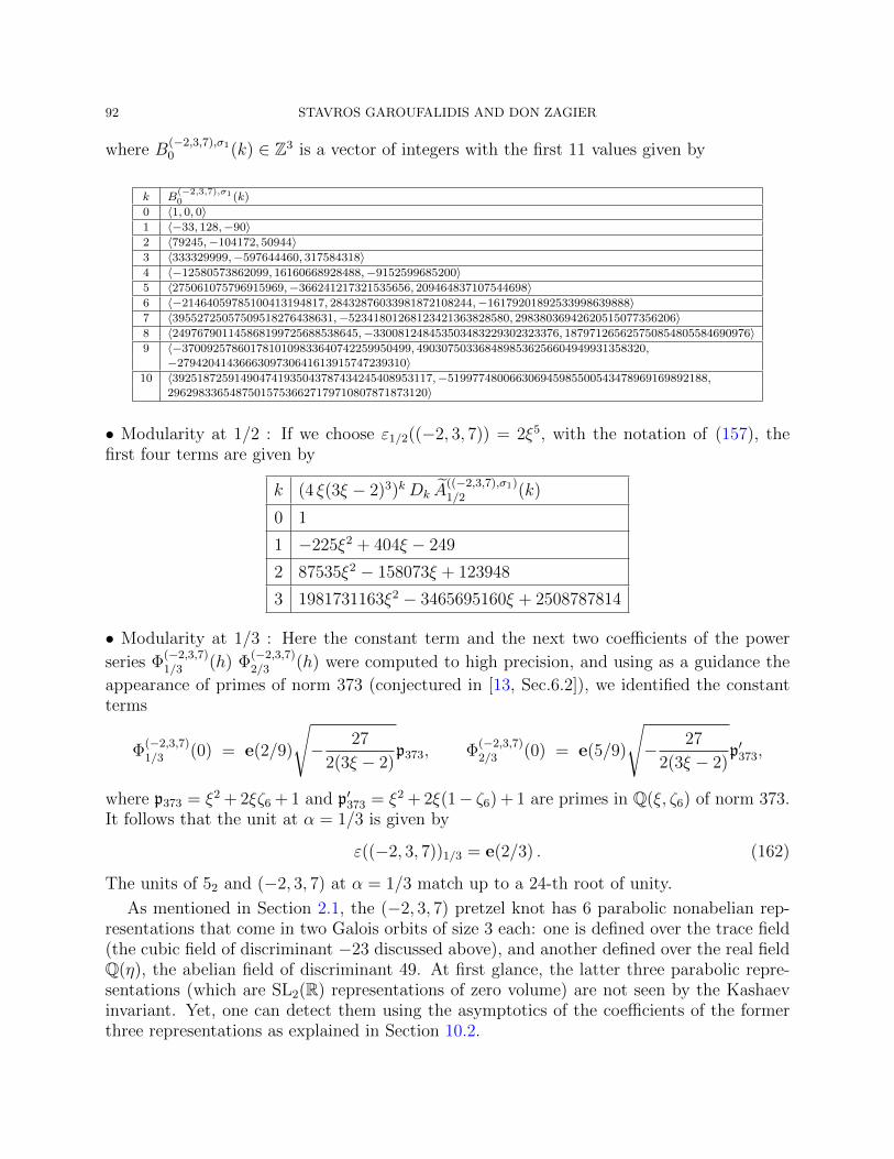
92 STAVROS GAROUFALIDIS AND DON ZAGIER
where B(−2,3,7),σ10 (k) ∈ Z3 is a vector of integers with the first 11 values given by
k B(−2,3,7),σ10 (k)
0 〈1, 0, 0〉1 〈−33, 128,−90〉2 〈79245,−104172, 50944〉3 〈333329999,−597644460, 317584318〉4 〈−12580573862099, 16160668928488,−9152599685200〉5 〈275061075796915969,−366241217321535656, 209464837107544698〉6 〈−21464059785100413194817, 28432876033981872108244,−16179201892533998639888〉7 〈39552725057509518276438631,−52341801268123421363828580, 29838036942620515077356206〉8 〈249767901145868199725688538645,−330081248453503483229302323376, 187971265625750854805584690976〉9 〈−3700925786017810109833640742259950499, 4903075033684898536256604949931358320,−2794204143666309730641613915747239310〉
10 〈392518725914904741935043787434245408953117,−519977480066306945985500543478969169892188,
296298336548750157536627179710807871873120〉
• Modularity at 1/2 : If we choose ε1/2((−2, 3, 7)) = 2ξ5, with the notation of (157), thefirst four terms are given by
k (4 ξ(3ξ − 2)3)kDk A((−2,3,7),σ1)1/2 (k)
0 1
1 −225ξ2 + 404ξ − 249
2 87535ξ2 − 158073ξ + 123948
3 1981731163ξ2 − 3465695160ξ + 2508787814
• Modularity at 1/3 : Here the constant term and the next two coefficients of the power
series Φ(−2,3,7)1/3 (h) Φ
(−2,3,7)2/3 (h) were computed to high precision, and using as a guidance the
appearance of primes of norm 373 (conjectured in [13, Sec.6.2]), we identified the constantterms
Φ(−2,3,7)1/3 (0) = e(2/9)
√− 27
2(3ξ − 2)p373, Φ
(−2,3,7)2/3 (0) = e(5/9)
√− 27
2(3ξ − 2)p′373,
where p373 = ξ2 + 2ξζ6 + 1 and p′373 = ξ2 + 2ξ(1− ζ6) + 1 are primes in Q(ξ, ζ6) of norm 373.It follows that the unit at α = 1/3 is given by
ε((−2, 3, 7))1/3 = e(2/3) . (162)
The units of 52 and (−2, 3, 7) at α = 1/3 match up to a 24-th root of unity.
As mentioned in Section 2.1, the (−2, 3, 7) pretzel knot has 6 parabolic nonabelian rep-resentations that come in two Galois orbits of size 3 each: one is defined over the trace field(the cubic field of discriminant −23 discussed above), and another defined over the real fieldQ(η), the abelian field of discriminant 49. At first glance, the latter three parabolic repre-sentations (which are SL2(R) representations of zero volume) are not seen by the Kashaevinvariant. Yet, one can detect them using the asymptotics of the coefficients of the formerthree representations as explained in Section 10.2.
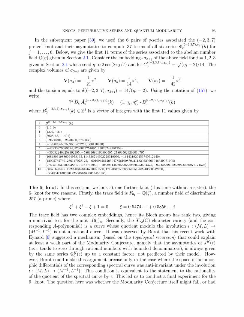
KNOTS, PERTURBATIVE SERIES AND QUANTUM MODULARITY 93
In the subsequent paper [39], we used the 6 pairs of q-series associated the (−2, 3, 7)
pretzel knot and their asymptotics to compute 37 terms of all six series Φ((−2,3,7),σj)0 (h) for
j = 1, . . . , 6. Below, we give the first 11 terms of the series associated to the abelian numberfield Q(η) given in Section 2.1. Consider the embeddings σ3+j of the above field for j = 1, 2, 3
given in Section 2.1 which send η to 2 cos(2πj/7) and let C((−2,3,7),σ3+j)0 =
√(ηj − 2)/14. The
complex volumes of σ3+j are given by
V(σ4) = − 1
21π2, V(σ5) =
1
14π2, V(σ6) = − 1
42π2
and the torsion equals to δ((−2, 3, 7), σ3+j) = 14/(ηj − 2). Using the notation of (157), wewrite
7kDk A((−2,3,7),σ3+j)0 (k) = (1, ηj, η
2j ) ·B
((−2,3,7),σ3+j)0 (k)
where B((−2,3,7),σ3+j)0 (k) ∈ Z3 is a vector of integers with the first 11 values given by
k B((−2,3,7),σ3+j)
0 (k)
0 〈1, 0, 0〉1 〈43, 0,−21〉2 〈3928, 63,−1491〉3 〈−9658210,−2570400, 8759835〉4 〈−12802855375, 9661452255, 660110430〉5 〈−42833879089694, 5736063757095, 23026249581258〉6 〈−360522404258392495,−58094689166990595, 278695629206010765〉7 〈108480519886094978165, 114336214602228319050,−161431920455740612440〉8 〈420957357301236147078125,−601694281205047856100870, 211820529501946639071105〉9 〈276051903390093831791757795950,−105329146895536652560323534375,−93062298372659896456977171525〉10 〈3837169849511929903158156720021580, 1712034755788650551262940860512280,
−3840647130863172583813306383456135〉
The 61 knot. In this section, we look at one further knot (this time without a sister), the61 knot for two reasons. Firstly, the trace field is F61 = Q(ξ), a number field of discriminant257 (a prime) where
ξ4 + ξ2 − ξ + 1 = 0, ξ = 0.5474 · · ·+ 0.5856 . . . i
The trace field has two complex embeddings, hence its Bloch group has rank two, givinga nontrivial test for the unit ε(61)α. Secondly, the SL2(C) character variety (and the cor-responding A-polynomial) is a curve whose quotient modulo the involution ι : (M,L) 7→(M−1, L−1) is not a rational curve. It was observed by Borot that his recent work withEynard [6] suggested a mechanism (based on the topological recursion) that could explainat least a weak part of the Modularity Conjecture, namely that the asymptotics of JK(ε)(as ε tends to zero through rational numbers with bounded denominators), is always givenby the same series ΦK
0 (ε) up to a constant factor, not predicted by their model. How-ever, Borot could make this argument precise only in the case where the space of holomor-phic differentials of the corresponding spectral curve was anti-invariant under the involutionι : (M,L) 7→ (M−1, L−1). This condition is equivalent to the statement to the rationalityof the quotient of the spectral curve by ι. This led us to conduct a final experiment for the61 knot. The question here was whether the Modularity Conjecture itself might fail, or had
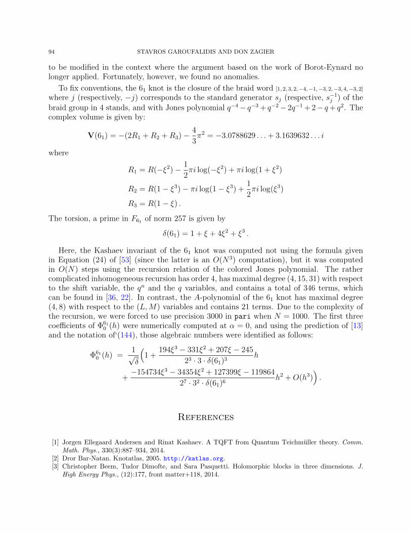
94 STAVROS GAROUFALIDIS AND DON ZAGIER
to be modified in the context where the argument based on the work of Borot-Eynard nolonger applied. Fortunately, however, we found no anomalies.
To fix conventions, the 61 knot is the closure of the braid word [1, 2, 3, 2,−4,−1,−3, 2,−3, 4,−3, 2]
where j (respectively, −j) corresponds to the standard generator sj (respective, s−1j ) of the
braid group in 4 stands, and with Jones polynomial q−4− q−3 + q−2− 2q−1 + 2− q+ q2. Thecomplex volume is given by:
V(61) = −(2R1 +R2 +R3)− 4
3π2 = −3.0788629 . . .+ 3.1639632 . . . i
where
R1 = R(−ξ2)− 1
2πi log(−ξ2) + πi log(1 + ξ2)
R2 = R(1− ξ3)− πi log(1− ξ3) +1
2πi log(ξ3)
R3 = R(1− ξ) .
The torsion, a prime in F61 of norm 257 is given by
δ(61) = 1 + ξ + 4ξ2 + ξ3 .
Here, the Kashaev invariant of the 61 knot was computed not using the formula givenin Equation (24) of [53] (since the latter is an O(N3) computation), but it was computedin O(N) steps using the recursion relation of the colored Jones polynomial. The rathercomplicated inhomogeneous recursion has order 4, has maximal degree (4, 15, 31) with respectto the shift variable, the qn and the q variables, and contains a total of 346 terms, whichcan be found in [36, 22]. In contrast, the A-polynomial of the 61 knot has maximal degree(4, 8) with respect to the (L,M) variables and contains 21 terms. Due to the complexity ofthe recursion, we were forced to use precision 3000 in pari when N = 1000. The first threecoefficients of Φ61
0 (h) were numerically computed at α = 0, and using the prediction of [13]and the notation of‘(144), those algebraic numbers were identified as follows:
Φ610 (h) =
1√δ
(1 +
194ξ3 − 331ξ2 + 207ξ − 245
23 · 3 · δ(61)3h
+−154734ξ3 − 34354ξ2 + 127399ξ − 119864
27 · 32 · δ(61)6h2 +O(h3)
).
References
[1] Jorgen Ellegaard Andersen and Rinat Kashaev. A TQFT from Quantum Teichmuller theory. Comm.Math. Phys., 330(3):887–934, 2014.
[2] Dror Bar-Natan. Knotatlas, 2005. http://katlas.org.[3] Christopher Beem, Tudor Dimofte, and Sara Pasquetti. Holomorphic blocks in three dimensions. J.
High Energy Phys., (12):177, front matter+118, 2014.
KNOTS, PERTURBATIVE SERIES AND QUANTUM MODULARITY 95
[4] Carl Bender and Steven Orszag. Advanced mathematical methods for scientists and engineers. McGraw-Hill Book Co., New York, 1978. International Series in Pure and Applied Mathematics.
[5] Sandro Bettin and Sary Drappeau. Modularity and value distribution of quantum invariants of hyper-bolic knots. Preprint 2019, arXiv:1905.02045.
[6] Gaetan Borot and Bertrand Eynard. All order asymptotics of hyperbolic knot invariants from non-perturbative topological recursion of A-polynomials. Quantum Topol., 6(1):39–138, 2015.
[7] David Boyd, Nathan Dunfield, and Fernando Rodriguez-Villegas. Mahler’s measure and the dilogarithm(II). Preprint 2005, arXiv:math.NT/0308041.
[8] Danny Calegari. Real places and torus bundles. Geom. Dedicata, 118:209–227, 2006.[9] Frank Calegari, Stavros Garoufalidis, and Don Zagier. Bloch groups, algebraic K-theory, units and
Nahm’s Conjecture. Preprint 2017, arXiv:1807.00957.[10] Daryl Cooper, Marc Culler, Henry Gillet, Daryl Long, and Peter Shalen. Plane curves associated to
character varieties of 3-manifolds. Invent. Math., 118(1):47–84, 1994.[11] Marc Culler, Nathan Dunfield, and Jeffrey Weeks. SnapPy, a computer program for studying the topol-
ogy of 3-manifolds. Available at http://snappy.computop.org (30/01/2015).[12] Tudor Dimofte, Davide Gaiotto, and Sergei Gukov. Gauge theories labelled by three-manifolds. Comm.
Math. Phys., 325(2):367–419, 2014.[13] Tudor Dimofte and Stavros Garoufalidis. The quantum content of the gluing equations. Geom. Topol.,
17(3):1253–1315, 2013.[14] Tudor Dimofte and Stavros Garoufalidis. Quantum modularity and complex Chern-Simons theory. Com-
mun. Number Theory Phys., 12(1):1–52, 2018.[15] Tudor Dimofte, Sergei Gukov, Jonatan Lenells, and Don Zagier. Exact results for perturbative Chern-
Simons theory with complex gauge group. Commun. Number Theory Phys., 3(2):363–443, 2009.[16] Nathan Dunfield and William Thurston. The virtual Haken conjecture: experiments and examples.
Geom. Topol., 7:399–441, 2003.[17] Tobias Ekholm, Angus Gruen, Sergei Gukov, Piotr Kucharski, Sunghyuk Park, and Piotr Sulkowski. Z
at large N : from curve counts to quantum modularity. Preprint 2020, arXiv:2005.13349.[18] Ludwig Faddeev. Discrete Heisenberg-Weyl group and modular group. Lett. Math. Phys., 34(3):249–254,
1995.[19] Ludwig Faddeev and Rinat Kashaev. Quantum dilogarithm. Modern Phys. Lett. A, 9(5):427–434, 1994.[20] Dongmin Gang, Seonhwa Kim, and Seokbeom Yoon. Adjoint Reidemeister torsions from wrapped M5-
branes. Preprint 2019, arXiv:1911.10718.[21] Stavros Garoufalidis. Chern-Simons theory, analytic continuation and arithmetic. Acta Math. Vietnam.,
33(3):335–362, 2008.[22] Stavros Garoufalidis. Twist knots data, 2010. http://people.mpim-bonn.mpg.de/stavros/
publications/twist.knot.data.[23] Stavros Garoufalidis. Pretzel knots data, 2012. http://people.mpim-bonn.mpg.de/stavros/
publications/pretzel.data.[24] Stavros Garoufalidis, Matthias Goerner, and Christian Zickert. The Ptolemy field of 3-manifold repre-
sentations. Algebr. Geom. Topol., 15(1):371–397, 2015.[25] Stavros Garoufalidis, Jie Gu, and Marcos Marino. Peacock patterns and resurgence in complex Chern-
Simons theory. Preprint 2020, arXiv:2012.00062.[26] Stavros Garoufalidis, Jie Gu, and Marcos Marino. The resurgent structure of quantum knot invariants.
Comm. Math. Phys., 386(1):469–493, 2021.[27] Stavros Garoufalidis and Rinat Kashaev. The descendant colored Jones polynomials. Preprint 2021,
arXiv:2108.07553.[28] Stavros Garoufalidis and Rinat Kashaev. Evaluation of state integrals at rational points. Commun.
Number Theory Phys., 9(3):549–582, 2015.[29] Stavros Garoufalidis and Rinat Kashaev. From state integrals to q-series. Math. Res. Lett., 24(3):781–
801, 2017.
96 STAVROS GAROUFALIDIS AND DON ZAGIER
[30] Stavros Garoufalidis, Rinat Kashaev, and Don Zagier. A modular quantum dilogarithm and invariantsof 3-manifolds. In preparation.
[31] Stavros Garoufalidis and Christoph Koutschan. The the non-commutative A-polynomial of (−2, 3, n)pretzel knots. Exp. Math., 2012.
[32] Stavros Garoufalidis and Christoph Koutschan. Irreducibility of q-difference operators and the knot 74.Algebr. Geom. Topol., 13(6):3261–3286, 2013.
[33] Stavros Garoufalidis and Thang T.Q. Le. The colored Jones function is q-holonomic. Geom. Topol.,9:1253–1293 (electronic), 2005.
[34] Stavros Garoufalidis, Eric Sabo, and Shane Scott. Exact computation of the n-loop invariants of knots.Exp. Math., 25(2):125–129, 2016.
[35] Stavros Garoufalidis, Peter Scholze, and Don Zagier. The Habiro ring of a number field. In preparation.[36] Stavros Garoufalidis and Xinyu Sun. The non-commutative A-polynomial of twist knots. J. Knot Theory
Ramifications, 19(12):1571–1595, 2010.[37] Stavros Garoufalidis, Dylan Thurston, and Christian Zickert. The complex volume of SL(n,C)-
representations of 3-manifolds. Duke Math. J., 164(11):2099–2160, 2015.[38] Stavros Garoufalidis and Roland van der Veen. Asymptotics of classical spin networks. Geom. Topol.,
17(1):1–37, 2013. With an appendix by Don Zagier.[39] Stavros Garoufalidis and Don Zagier. Knots and their related q-series. Preprint 2021.[40] Stavros Garoufalidis and Don Zagier. Resummation of factorially divergent series. Preprint 2021.[41] Stavros Garoufalidis and Don Zagier. Asymptotics of Nahm sums at roots of unity. Ramanujan J.,
55(1):219–238, 2021.[42] Sebastian Goette and Christian Zickert. The extended Bloch group and the Cheeger-Chern-Simons class.
Geom. Topol., 11:1623–1635, 2007.[43] Daniel Grunberg and Pieter Moree. Sequences of enumerative geometry: congruences and asymptotics.
Experiment. Math., 17(4):409–426, 2008. With an appendix by Don Zagier.[44] Sergei Gukov. Three-dimensional quantum gravity, Chern-Simons theory, and the A-polynomial. Comm.
Math. Phys., 255(3):577–627, 2005.[45] Sergei Gukov, Marcos Marino, and Pavel Putrov. Resurgence in complex Chern-Simons theory. Preprint
2016, arXiv:1605.07615.[46] Sergei Gukov, Du Pei, Pavel Putrov, and Cumrun Vafa. BPS spectra and 3-manifold invariants. J. Knot
Theory Ramifications, 29(2):2040003, 85, 2020.[47] Kazuo Habiro. On the quantum sl2 invariants of knots and integral homology spheres. In Invariants
of knots and 3-manifolds (Kyoto, 2001), volume 4 of Geom. Topol. Monogr., pages 55–68 (electronic).Geom. Topol. Publ., Coventry, 2002.
[48] Kazuhiro Hikami. Generalized volume conjecture and the A-polynomials: the Neumann-Zagier potentialfunction as a classical limit of the partition function. J. Geom. Phys., 57(9):1895–1940, 2007.
[49] Friedrich Hirzebruch and Don Zagier. The Atiyah-Singer theorem and elementary number theory. Publishor Perish, Inc., Boston, Mass., 1974. Mathematics Lecture Series, No. 3.
[50] Jun-ichi Igusa. Theta functions. Springer-Verlag, New York-Heidelberg, 1972. Die Grundlehren dermathematischen Wissenschaften, Band 194.
[51] Vaughan Jones. Hecke algebra representations of braid groups and link polynomials. Ann. of Math. (2),126(2):335–388, 1987.
[52] Rinat Kashaev. A link invariant from quantum dilogarithm. Modern Phys. Lett. A, 10(19):1409–1418,1995.
[53] Rinat Kashaev. The hyperbolic volume of knots from the quantum dilogarithm. Lett. Math. Phys.,39(3):269–275, 1997.
[54] Rinat Kashaev, Vladimir Mangazeev, and Yuri Stroganov. Star-square and tetrahedron equations inthe Baxter-Bazhanov model. Internat. J. Modern Phys. A, 8(8):1399–1409, 1993.
[55] Maxim Kontsevich. Talks on resurgence. July 20, 2020 and August 21, 2020.[56] John Lewis and Don Zagier. Period functions for Maass wave forms. I. Ann. of Math. (2), 153(1):191–
258, 2001.
KNOTS, PERTURBATIVE SERIES AND QUANTUM MODULARITY 97
[57] Hitoshi Murakami and Jun Murakami. The colored Jones polynomials and the simplicial volume of aknot. Acta Math., 186(1):85–104, 2001.
[58] Walter Neumann. Combinatorics of triangulations and the Chern-Simons invariant for hyperbolic 3-manifolds. In Topology ’90 (Columbus, OH, 1990), volume 1 of Ohio State Univ. Math. Res. Inst. Publ.,pages 243–271. de Gruyter, Berlin, 1992.
[59] Walter Neumann. Extended Bloch group and the Cheeger-Chern-Simons class. Geom. Topol., 8:413–474,2004.
[60] Walter Neumann and Don Zagier. Volumes of hyperbolic three-manifolds. Topology, 24(3):307–332, 1985.[61] Tomotada Ohtsuki. A polynomial invariant of rational homology 3-spheres. Invent. Math., 123(2):241–
257, 1996.[62] Hans Rademacher. Zur Theorie der Dedekindschen Summen. Math. Z., 63:445–463, 1956.[63] Andrei Suslin. K3 of a field, and the Bloch group. volume 183, pages 180–199, 229. 1990. Translated
in Proc. Steklov Inst. Math. 1991, no. 4, 217–239, Galois theory, rings, algebraic groups and theirapplications (Russian).
[64] William Thurston. The geometry and topology of 3-manifolds. Universitext. Springer-Verlag, Berlin,1977. Lecture notes, Princeton.
[65] Vladimir Turaev. The Yang-Baxter equation and invariants of links. Invent. Math., 92(3):527–553, 1988.[66] Roland van der Veen. Proof of the volume conjecture for Whitehead chains. Acta Math. Vietnam.,
33(3):421–431, 2008.[67] Masha Vlasenko and Sander Zwegers. Nahm’s conjecture: asymptotic computations and counterexam-
ples. Commun. Number Theory Phys., 5(3):617–642, 2011.[68] Herbert S. Wilf and Doron Zeilberger. An algorithmic proof theory for hypergeometric (ordinary and
“q”) multisum/integral identities. Invent. Math., 108(3):575–633, 1992.[69] Edward Witten. Searching for new invariants of 4-manifolds and knots. January 2020, Auckland New
Zealand.[70] Edward Witten. Two lectures on the Jones polynomial and Khovanov homology. In Lectures on geometry,
Clay Lect. Notes, pages 1–27. Oxford Univ. Press, Oxford, 2017.[71] Don Zagier. Holomorphic quantum modular forms. In preparation.[72] Don Zagier. The dilogarithm function. In Frontiers in number theory, physics, and geometry. II, pages
3–65. Springer, Berlin, 2007.[73] Don Zagier. Quantum modular forms. In Quanta of maths, volume 11 of Clay Math. Proc., pages
659–675. Amer. Math. Soc., Providence, RI, 2010.[74] Don Zagier and Herbert Gangl. Classical and elliptic polylogarithms and special values of L-series. In
The arithmetic and geometry of algebraic cycles (Banff, AB, 1998), volume 548 of NATO Sci. Ser. CMath. Phys. Sci., pages 561–615. Kluwer Acad. Publ., Dordrecht, 2000.
[75] Christian Zickert. The volume and Chern-Simons invariant of a representation. Duke Math. J.,150(3):489–532, 2009.
[76] Christian Zickert. The extended Bloch group and algebraic K-theory. J. Reine Angew. Math., 704:21–54,2015.
International Center for Mathematics, Department of Mathematics, Southern Univer-sity of Science and Technology, Shenzhen, Chinahttp://people.mpim-bonn.mpg.de/stavros
Email address: [email protected]
Max Planck Institute for Mathematics, 53111 Bonn, Germanyhttp://people.mpim-bonn.mpg.de/zagier
Email address: [email protected]

![[Tutorial] Modular Forms - PARI/GP · Modular forms attached toHecke characterson imaginary and real quadratic fields. Modular forms associated toelliptic curvesby Wiles’s modularity](https://static.fdocument.org/doc/165x107/5f5af59a26f27b13500199d4/tutorial-modular-forms-parigp-modular-forms-attached-tohecke-characterson-imaginary.jpg)