SIAM J. NUMER. ANAL. c© 2009 Society for Industrial and Applied MathematicsVol. 47, No. 3, pp. 1952–1970

PERTURBATIVE ANALYSIS OF THE METHOD OF PARTICULARSOLUTIONS FOR IMPROVED INCLUSION OF HIGH-LYING

DIRICHLET EIGENVALUES∗

A. H. BARNETT†

Abstract. The Dirichlet eigenvalue or “drum” problem in a domain Ω ⊂ R2 becomes numerically

challenging at high eigenvalue (frequency) E. In this regime the method of particular solutions (MPS)gives spectral accuracy for many domain shapes. It requires a number of degrees of freedom scalingas

√E, the number of wavelengths on the boundary, in contrast to direct discretization for which

this scaling is E. Our main result is an inclusion bound on eigenvalues that is a factor O(√

E) tighterthan the classical bound of Moler–Payne and that is optimal in that it reflects the true slopes ofcurves appearing in the MPS. We also present an MPS variant that cures a normalization problem inthe original method, while evaluating basis functions only on the boundary. This method is efficientat high frequencies, where we show that, in practice, our inclusion bound can give three extra digitsof eigenvalue accuracy with no extra effort.

Key words. particular solutions, eigenvalue, Dirichlet, drum, Laplacian, inclusion

AMS subject classifications. 35P15, 47A55, 65N35, 65N15

DOI. 10.1137/080724022

1. Introduction and main results. Computing the eigenvalues and eigen-modes of the Laplace operator with homogeneous boundary condition (BC) in abounded domain Ω ⊂ Rd for d = 2, 3, . . . is a classical problem with a 150-year-long history; for reviews, see [30, 43]. It has a wealth of applications in physics andengineering including the vibration of membranes (drums), resonances and modes ofacoustic, electromagnetic, and optical cavities and waveguides, energy states of quan-tum particles, and data analysis [40]. We focus on the case of a Dirichlet BC, i.e.,acoustically sound-soft walls. The spectrum σD := {Ej}∞j=1 and modes {φj}∞j=1 aredefined by

−Δφj = Ejφj in Ω,(1.1)φj = 0 on ∂Ω .(1.2)

Physically the eigenvalues can be interpreted as frequencies; we order them (includingmultiplicities) E1 < E2 ≤ E3 ≤ · · · . We may choose orthonormal modes, that is,(φi, φj)Ω :=

∫Ωφiφj dx = δij for all i, j = 1, 2, . . . , where δ is the Kronecker delta.

There has been a growing interest in the computationally demanding case of higheigenvalue (high mode number j), where many wavelengths span the domain. Oneexample is dielectric microcavity lasers, where the use of asymmetric shapes has led tomuch higher output powers; to predict lasing [45], a large number of cavity resonances(which can be approximated by Dirichlet modes) are needed at j > 103. More broadly,the field of “quantum chaos” (short-wavelength asymptotic study of modes of systemswith chaotic ray dynamics) has blossomed in the last 20 years in both physics [22](with applications such as atomic physics and quantum dots) and mathematics (e.g.,

∗Received by the editors May 13, 2008; accepted for publication (in revised form) January 5, 2009;published electronically May 27, 2009. This work was supported in part by a Courant Instructorshipat NYU and by NSF grant DMS-0507614.

http://www.siam.org/journals/sinum/47-3/72402.html†Department of Mathematics, Dartmouth College, Hanover, NH 03755 (ahb@math.dartmouth.

edu).

1952

PERTURBATIVE INCLUSION OF DIRICHLET EIGENVALUES 1953

quantum ergodicity [47] and arithmetic manifolds). Numerical investigation has beena vital part of this endeavor [1, 4] and has led to discoveries such as “scars” of periodicray orbits in the modes [25].

The method of particular solutions (MPS), also known as collocation or “pointmatching,” uses basis functions that satisfy the Helmholtz equation (1.1) but notnecessarily (1.2). It was originally used by Fox, Henrici, and Moler [16] to computelow eigenvalues of an L-shaped domain to 8 digit accuracy, and has been improved bymany, including Kuttler and Sigillito [29], and recently by Betcke and Trefethen [5].Much of the key early analysis of the MPS appeared in SINUM [16, 33, 41, 10]. Forgeometries with many corners, a domain decomposition version was pioneered byDescloux and Tolley [8], modified by Driscoll [9] to find eigenvalues of the well-knownpair of Gordon–Wolpert–Webb isospectral drums [21] to high accuracy, and furtherimproved by Betcke [6]. In physics, where the emphasis is on high frequencies, relatedmethods of Heller [25, 26] and the very efficient “scaling method” of Vergini andSaraceno [46, 3, 4] have enjoyed unrivaled success. In this regime the advantage ofthe MPS is that the basis size scales (in d = 2) as the wavenumber

√E (e.g., see [2]),

rather than E as with finite difference or finite element methods. (This advantage isshared by boundary integral methods [1]).

In the MPS a solution to (1.1) is approximated by a linear combination of ba-sis functions {ξn}n=1,...,N , each of which satisfies −Δξn = Eξn in Ω at some trialfrequency parameter E but which do not individually satisfy the Dirichlet BC. Pop-ular basis functions are plane waves [26], corner-adapted Fourier–Bessel functions[16, 9, 5, 6], and fundamental solutions [12, 27, 4]. If a trial solution u ∈ Span{ξn}satisfies u = 0 on ∂Ω while u �= 0 in Ω, then it must be a multiple of a mode φjfor some j, and we must have E = Ej . In practice, this is rarely achieved exactly.However, by defining the boundary error measure (or “tension”)

(1.3) t = t[u] :=‖u‖∂Ω

‖u‖Ω,

where ‖u‖∂Ω and ‖u‖Ω are the usual L2-norms on the boundary and interior, respec-tively, we have the following inclusion bound from a theorem of Moler–Payne [33, 29].Let −Δu = Eu in Ω, then there exists an eigenvalue Ej satisfying

(1.4)|E − Ej |Ej

≤ C′Ωt[u] ,

where C′Ω is a constant depending only on the domain. (C′

Ω is an a priori upperbound on ‖h‖Ω/‖h‖∂Ω for harmonic functions h [29], hence (1.4) is known as an apriori-a posteriori inequality [30].) Eigenvalues may then be identified by searchingthe frequency (E) axis for local minima of the function

(1.5) tm(E) := minu∈Span{ξn}

t[u] ,

as shown in Figure 1.1. Similar curves appear in [5, 7, 11]. Equation (1.4) statesthat the eigenvalue accuracy which may be claimed is controlled by the size of theminimum found.

However, observations of the slopes of curves such as Figure 1.1 led the authorto notice that the Moler–Payne bounds are not optimal at high E. It turns out that,for E in the neighborhood of each eigenvalue Ej , the bounds can be made a factor of√E tighter, as follows.

1954 A. H. BARNETT

10 20 30 40 50 60 70 80 90 1000

0.2

0.4

0.6

E

t m(E

)

1 2 3 4 5 6 7 8 9 10 11 1213 14 15 16 17 18 1920 21

Theorem 1.1

Moler−Payne

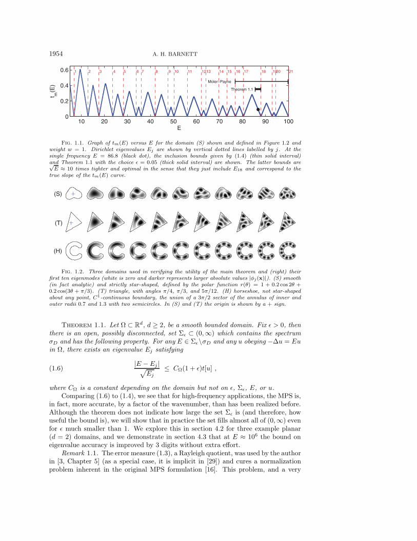
Fig. 1.1. Graph of tm(E) versus E for the domain (S) shown and defined in Figure 1.2 andweight w = 1. Dirichlet eigenvalues Ej are shown by vertical dotted lines labelled by j. At thesingle frequency E = 86.8 (black dot), the inclusion bounds given by (1.4) (thin solid interval)and Theorem 1.1 with the choice ε = 0.05 (thick solid interval) are shown. The latter bounds are√

E ≈ 10 times tighter and optimal in the sense that they just include E18 and correspond to thetrue slope of the tm(E) curve.

(H)

(T)

(S)

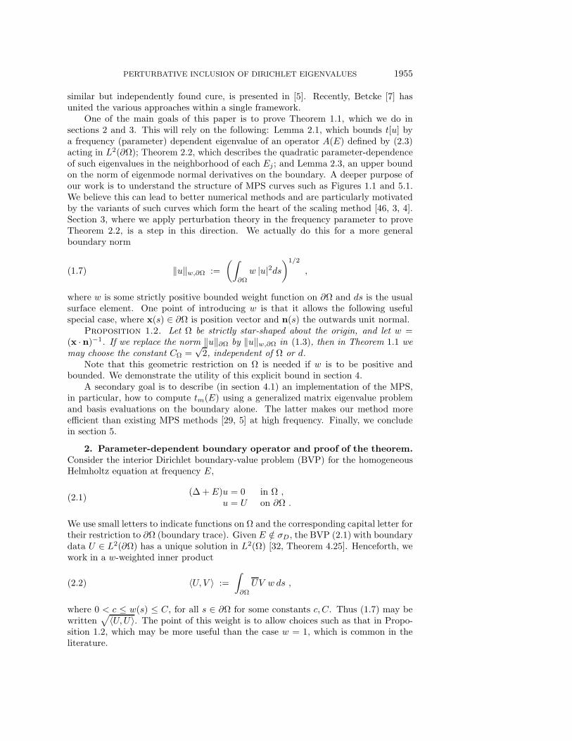
Fig. 1.2. Three domains used in verifying the utility of the main theorem and (right) theirfirst ten eigenmodes (white is zero and darker represents larger absolute values |φj(x)|). (S) smooth(in fact analytic) and strictly star-shaped, defined by the polar function r(θ) = 1 + 0.2 cos 2θ +0.2 cos(3θ + π/3). (T) triangle, with angles π/4, π/3, and 5π/12. (H) horseshoe, not star-shapedabout any point, C1-continuous boundary, the union of a 3π/2 sector of the annulus of inner andouter radii 0.7 and 1.3 with two semicircles. In (S) and (T) the origin is shown by a + sign.

Theorem 1.1. Let Ω ⊂ Rd, d ≥ 2, be a smooth bounded domain. Fix ε > 0, thenthere is an open, possibly disconnected, set Σε ⊂ (0,∞) which contains the spectrumσD and has the following property. For any E ∈ Σε\σD and any u obeying −Δu = Euin Ω, there exists an eigenvalue Ej satisfying

(1.6)|E − Ej |√

Ej≤ CΩ(1 + ε)t[u] ,

where CΩ is a constant depending on the domain but not on ε, Σε, E, or u.Comparing (1.6) to (1.4), we see that for high-frequency applications, the MPS is,

in fact, more accurate, by a factor of the wavenumber, than has been realized before.Although the theorem does not indicate how large the set Σε is (and therefore, howuseful the bound is), we will show that in practice the set fills almost all of (0,∞) evenfor ε much smaller than 1. We explore this in section 4.2 for three example planar(d = 2) domains, and we demonstrate in section 4.3 that at E ≈ 106 the bound oneigenvalue accuracy is improved by 3 digits without extra effort.

Remark 1.1. The error measure (1.3), a Rayleigh quotient, was used by the authorin [3, Chapter 5] (as a special case, it is implicit in [29]) and cures a normalizationproblem inherent in the original MPS formulation [16]. This problem, and a very

PERTURBATIVE INCLUSION OF DIRICHLET EIGENVALUES 1955

similar but independently found cure, is presented in [5]. Recently, Betcke [7] hasunited the various approaches within a single framework.

One of the main goals of this paper is to prove Theorem 1.1, which we do insections 2 and 3. This will rely on the following: Lemma 2.1, which bounds t[u] bya frequency (parameter) dependent eigenvalue of an operator A(E) defined by (2.3)acting in L2(∂Ω); Theorem 2.2, which describes the quadratic parameter-dependenceof such eigenvalues in the neighborhood of each Ej ; and Lemma 2.3, an upper boundon the norm of eigenmode normal derivatives on the boundary. A deeper purpose ofour work is to understand the structure of MPS curves such as Figures 1.1 and 5.1.We believe this can lead to better numerical methods and are particularly motivatedby the variants of such curves which form the heart of the scaling method [46, 3, 4].Section 3, where we apply perturbation theory in the frequency parameter to proveTheorem 2.2, is a step in this direction. We actually do this for a more generalboundary norm

(1.7) ‖u‖w,∂Ω :=(∫

∂Ω

w |u|2ds)1/2

,

where w is some strictly positive bounded weight function on ∂Ω and ds is the usualsurface element. One point of introducing w is that it allows the following usefulspecial case, where x(s) ∈ ∂Ω is position vector and n(s) the outwards unit normal.

Proposition 1.2. Let Ω be strictly star-shaped about the origin, and let w =(x · n)−1. If we replace the norm ‖u‖∂Ω by ‖u‖w,∂Ω in (1.3), then in Theorem 1.1 wemay choose the constant CΩ =

√2, independent of Ω or d.

Note that this geometric restriction on Ω is needed if w is to be positive andbounded. We demonstrate the utility of this explicit bound in section 4.

A secondary goal is to describe (in section 4.1) an implementation of the MPS,in particular, how to compute tm(E) using a generalized matrix eigenvalue problemand basis evaluations on the boundary alone. The latter makes our method moreefficient than existing MPS methods [29, 5] at high frequency. Finally, we concludein section 5.

2. Parameter-dependent boundary operator and proof of the theorem.Consider the interior Dirichlet boundary-value problem (BVP) for the homogeneousHelmholtz equation at frequency E,

(2.1)(Δ + E)u = 0 in Ω ,

u = U on ∂Ω .

We use small letters to indicate functions on Ω and the corresponding capital letter fortheir restriction to ∂Ω (boundary trace). Given E /∈ σD, the BVP (2.1) with boundarydata U ∈ L2(∂Ω) has a unique solution in L2(Ω) [32, Theorem 4.25]. Henceforth, wework in a w-weighted inner product

(2.2) 〈U, V 〉 :=∫∂Ω

UV w ds ,

where 0 < c ≤ w(s) ≤ C, for all s ∈ ∂Ω for some constants c, C. Thus (1.7) may bewritten

√〈U,U〉. The point of this weight is to allow choices such as that in Propo-sition 1.2, which may be more useful than the case w = 1, which is common in theliterature.

1956 A. H. BARNETT

The parameter-dependent operator A = A(E) is defined by

(2.3) 〈U,A(E)V 〉 = (u, v)Ω , for all U, V ∈ L2(∂Ω).

(By v we mean the unique interior solution to (2.1) with data V ). A unique suchoperator in L2(∂Ω) exists by the Riesz representation theorem. By (2.3), it is positiveand self-adjoint (in the w-weighted norm) for real E. Treating (1.4) as an upperbound on ‖u‖Ω, it follows that A(E) is bounded for all E /∈ σD. An interpretationof A is that its sesquilinear form encodes the domain inner product of the interiorHelmholtz extensions of two given boundary functions.

An inverse eigenvalue λ(E) of A is defined at each E /∈ σD by

(2.4) A(E)X(E) =1

λ(E)X(E) ,

with corresponding eigenfunction 0 �= X(E) ∈ L2(∂Ω). We are interested in howthe (inverse) spectrum of A(E) depends on E. At this point we might stop to askwhether A even possesses a point spectrum. (2.1) has a solution operator K whichmaps U to u. For smooth domains (C∞ boundary), K is bounded from L2(∂Ω) toH1/2(Ω) (e.g., see [31]), thus by standard Sobolev embedding theorems, is compactfrom L2(∂Ω) to L2(Ω). Since A = K∗K, where K∗ is the adjoint with respect to theappropriate inner products, A is compact. Thus A has pure point spectrum, and thesequence {λi(A)}i=1,2,... has no accumulation point. If Ω has corners, we expect (andhave numerical evidence) that A remains compact but do not yet know a proof.

The w-weighted version of (1.3) is (we retain the same symbol)

(2.5) t[u] :=‖u‖w,∂Ω

‖u‖Ω.

For general w, we have the following simple lower bound on t[u] in terms of theparameter-dependent spectrum of A(E).

Lemma 2.1. Let λ1(E) be the lowest inverse eigenvalue of A(E) defined by (2.4).Fix E > 0, then for all u obeying −Δu = Eu in Ω, it holds that

(2.6) t[u] ≥√λ1(E) ,

where t[u] is defined by (2.5).Proof. Since A is self-adjoint and bounded,

(2.7) ‖u‖2Ω = 〈U,AU〉 ≤ 1

λ1‖U‖2

w,∂Ω ,

and the proof follows from the definition (2.5).We now describe the behavior of this lowest inverse eigenvalue for parameter

values E in the neighborhood of the Dirichlet spectrum of Ω. We will make frequentuse of the weighted eigenmode boundary functions

(2.8) ψj :=1w∂nφj ,

where ∂nφj := n · ∇φj |∂Ω is the usual normal derivative. These turn out to be thenatural boundary representation of modes associated with the norm (1.7). We alsoneed the infinite matrix Q = (Qij) whose entries are the weighted mode boundaryinner products

(2.9) Qij := 〈ψi, ψj〉 , i, j = 1, 2, . . . .

The proof of the following theorem is more involved and is the purpose of section 3.

PERTURBATIVE INCLUSION OF DIRICHLET EIGENVALUES 1957

Theorem 2.2. Fix j ∈ N, and let p be the (finite) multiplicity of Ej. Withoutloss of generality choose j to be the first in the list of degenerate eigenvalues, that is,Ej = Ej+1 = · · · = Ej+p−1. Then in the limit as E tends to Ej , precisely p inverseeigenvalues of A(E) vanish in the following fashion:

(2.10) λi(E) = c(i)j (E − Ej)2 +O

((E − Ej)4

), i = 1, . . . , p,

where the curvature coefficients c(1)j ≤ c

(2)j ≤ · · · ≤ c

(p)j are given by the inverse

eigenvalues of the p × p submatrix Q := (Qik)i,k=j,...,j+p−1. The smallest coefficientsatisfies

(2.11)1

c(1)j

= supφ∈Φ,‖φ‖Ω=1

∫∂Ω

1w|∂nφ|2ds ,

where Φ := Span{φj , . . . , φj+p−1} is the Ej-eigenspace.This locally quadratic behavior of the smallest inverse eigenvalue λ1(E) versus

frequency E is visible in Figure 1.1: tm(E) is a good approximation to√λ1(E) and

appears locally linear. Note that when Ej is a simple eigenvalue (p = 1), this gives

(2.12)1

c(1)j

= ‖ψj‖2w,∂Ω =

∫∂Ω

1w|∂nφj |2ds .

The right-most expressions in (2.11) and (2.12) are now bounded above because ofthe following, which puts a limit on how “shallow” the parabola λ1(E) may be.

Lemma 2.3 (Rellich). Given a bounded Lipschitz domain Ω ⊂ Rd, there areconstants Cw,Ω ≥ cw,Ω > 0 depending only on Ω and the weight w, such that

(2.13) c2w,ΩEj ≤∫∂Ω

1w|∂nφj |2ds ≤ C2

w,ΩEj for all j = 1, 2, . . . .

For the special case w = (x · n)−1, one may choose cw,Ω = Cw,Ω =√

2, independentof Ω, in which case the inequalities become an equality.

The inequalities are proved in Hassell–Tao [24, section 2] in the case w = 1 and∂Ω smooth but carry over trivially to strictly positive bounded w. The lower bounduses (2.14) below, thus holds for Lipschitz domains. They derived the upper boundusing commutator estimates involving a smooth vector field which points normallyoutwards on ∂Ω. (Also see [19, Lemma 2.1] for the case of domains with a Lipschitznormal vector field.) A simple generalization of this vector field construction to besmooth with merely positive normal component on ∂Ω allows the upper bound tocarry over to Lipschitz domains. For instance, the vector field x works for strictlystar-shaped Lipschitz domains [23]. The special-weight case in Lemma 2.3 is due toRellich [38], who proved

(2.14)∫∂Ω

x · n |∂nφ|2ds = 2Ej

for any bounded Ω and dimension d (regardless of whether Ω is star-shaped).Remark 2.1. The argument and Remark of [24, section 2] carries over to the case

of Ω possessing a boundary of only C1 continuity, since the first derivatives of theconstructed vector field remain bounded. Therefore, with w = 1, we get that Cw,Ω isthe inverse of the largest δ such that the function r(x) = dist(x, ∂Ω), x ∈ Ω, is C1

continuous wherever r ∈ [0, δ]. For domain (H) of Figure 1.2, this gives Cw,Ω = 10/3,the inverse of the minimum radius of curvature.

1958 A. H. BARNETT

2.1. Proof of main theorem. We now have all the pieces to prove Theorem 1.1,more precisely, its generalization to general strictly positive bounded weight w. For agiven eigenmode number j, Theorem 2.2 implies that limE→Ej c

(1)j (E−Ej)2/λ1(E) =

1, thus there is a δj > 0 such that

(2.15)

√c(1)j

λ1(E)|E − Ej | ≤ 1 + ε

holds for all E in the punctured interval 0 < |E − Ej | < δj . By choosing Σε =⋃∞j=1{E : |E −Ej | < δj}, then for each E ∈ Σε \ σD, there exists a j such that (2.15)

holds. Substituting into (2.15), the bound from Lemma 2.1 and the upper bound inLemma 2.3 completes the proof of Theorem 1.1, with the constant CΩ being equal tothe upper constant Cw,Ω in Lemma 2.3.

Remark 2.2. Theorem 2.2 is stronger than necessary for this proof, since onlythe existence of limE→Ej c

(1)j (E − Ej)2/λ1(E) is needed. In fact, the full analyticity

of λ1(E) will be proved in section 3.

3. Proof of quadratic behavior of inverse eigenvalues of A. Here (withAppendices A and B) we prove Theorem 2.2. The first part involves a modal expan-sion, which allows us to split the operator A(E) into a finite-rank part associated withthe jth eigenspace, and a remainder, which we show is analytic in the parameter E inthe neighborhood of Ej . We then apply Rellich–Kato analytic operator perturbationtheory to show that the inverse eigenvalues {λi(E)}i=1,...,p have quadratic behaviorabout Ej . However, there is a twist: the needed eigenvalue(s) of A(E) have poles atE = Ej . This we may cancel by scalar multiplication, but the price to pay is that an-alytic perturbation theory is no longer applicable to the resulting infinite multiplicityzero eigenvalue. Nevertheless, the Cauchy interlacing property will recover what isneeded.

3.1. Mode expansion of the boundary operator. The key to our proof isto express our boundary operator A as an infinite sum of rank-1 operators associatedwith each eigenmode boundary function.

Lemma 3.1.

(3.1) A(E) =∞∑j=1

ψj〈ψj , ·〉(E − Ej)2

.

Remark 3.1. A similar formula (for the casew = 1) is known [34] for the Dirichlet-to-Neumann map for (2.1). In fact, when w = 1 it can be shown directly that −A(E)is the E-derivative of the Dirichlet-to-Neumann map [17, equation (2.5)].

Proof. The Helmholtz equation Green’s function G in the domain Ω is defined by[18]:

(3.2)(−Δx − E)G(x,y) = δ(x − y) for x,y ∈ Ω,

G(x,y) = 0 for x ∈ ∂Ω or y ∈ ∂Ω.

G depends on E, although we shall not indicate this explicitly. δ is the Dirac deltadistribution in Rd. Then the solution operator K for the BVP (2.1) is

(3.3) u(x) = (KU)(x) =∫∂Ω

K(x, s)U(s) ds for x ∈ Ω ,

PERTURBATIVE INCLUSION OF DIRICHLET EIGENVALUES 1959

where s ∈ ∂Ω is a boundary coordinate and the Poisson kernel for the Helmholtzequation is

(3.4) K(x, s) = ∂n(s)G(x, s),

where here ∂n(s) indicates the normal derivative with respect to the second argument,evaluated at the boundary point s. From (3.3) we get

(3.5) (u, v)Ω =∫∂Ω

∫∂Ω

U(s)V (s′)∫

Ω

∂n(s)G(x, s)∂n(s′)G(x, s′) dx dsds′ .

Since (2.3) holds for arbitrary U, V ∈ L2(∂Ω), we may write the action of A on anyV ∈ L2(∂Ω) as the integral operator (AV )(s) =

∫∂ΩA(s, s′)V (s′) ds′ whose kernel is

(3.6) A(s, s′) =1

w(s)

∫Ω

∂n(s)G(x, s)∂n(s′)G(x, s′) dx.

Inserting the usual eigenfunction expansion [18]

(3.7) G(x,y) =∞∑j=1

φj(x)φj(y)E − Ej

into (3.6), orthonormality on Ω kills the domain integral and one of the sums, leaving

(3.8) A(s, s′) =1

w(s)

∞∑j=1

∂nφj(s) ∂nφj(s′)(E − Ej)2

.

The apparent lack of symmetry of the kernel is deceptive and is merely a result ofthe weighted inner product (2.2). It is simple to check that this kernel is equivalentto the desired symmetric formula (3.1).

Remark 3.2. Despite its suggestive form, (3.1) is not a sum of orthogonal pro-jections, nor a spectral representation, since {ψj} are not unit norm and, althoughcomplete in L2(∂Ω), they are generally not orthogonal.

Remark 3.3. Although each term in (3.1) is a bounded operator, with boundC2w,ΩEj/(E − Ej)2 following from Lemma 2.3, the sum of these bounds is divergent

for all d ≥ 2. This follows from Weyl’s law [18, Chapter 11], which states that asymp-totically, the number of Laplacian eigenvalues below E grows like Ed/2. Therefore,(3.1) cannot directly be used to show that A is the norm limit of finite-rank operatorsand hence compact.

3.2. Perturbation theory for inverse eigenvalues. From now on we fix themode number j, with multiplicity p. Recall if p > 1, then for convenience, j is chosento be the lowest in the degenerate set j, . . . , j + p− 1. It is a standard result that pis finite, since the Laplacian has compact inverse [13, section 6.5.1]. We separate theterms in the sum (3.1) associated with this set, giving

(3.9) (E − Ej)2A(E) = Bj + (E − Ej)2Aj(E) ,

where the fixed rank-p operator associated with the Ej-eigenspace is

(3.10) Bj :=p∑

m=1

ψj+m−1〈ψj+m−1, ·〉

1960 A. H. BARNETT

and the remainder is a scalar multiple of the bounded operator

(3.11) Aj(E) :=∑

m∈N,m/∈[j,j+p−1]

ψm〈ψm, ·〉(E − Em)2

.

With respect to the parameter E, the latter operator has second-order poles at alleigenvalues not equal to Ej . It is also analytic near Ej (the proof is in Appendix A).

Lemma 3.2. Aj(E) is a bounded regular (analytic) operator in the sense of Rellich[39, p. 55] for E in a neighborhood of Ej. That is, for each f ∈ L2(∂Ω), the elementAj(E)f exists as a power series f0 + (E − Ej)f1 + (E − Ej)2f2 + · · · convergent inL2(∂Ω) for E in a neighborhood of Ej.

Now define {μi(E)} to be the set of parameter-dependent eigenvalues of the op-erator (E −Ej)2A(E). We wish to understand their behavior when E is close to Ej ,since from them we can simply recover the desired λ(E) as defined in (2.4). We firstcharacterize the eigenvalues of Bj in terms of Q, the mode boundary inner productmatrix for the eigenspace.

Lemma 3.3. Bj has (counting multiplicity) precisely p nonzero eigenvalues ν1 ≥ν2 ≥ · · · ≥ νp, which are identical to the set of eigenvalues (counting multiplicity)of the matrix Q defined by Theorem 2.2 and (2.9). Bj also has a zero eigenvalue ofinfinite multiplicity.

Proof. Given β := (β1, . . . , βp)T , define φ =∑p

m=1 βmφj+m−1, then by orthonor-mality ‖φ‖Ω = |β|, the usual Euclidean norm in Cp. Thus φ is an L2(Ω)-normalizedeigenmode whenever |β| = 1. Its weighted normal derivative is ψ = 1

w∂nφ. Then,using (2.9) and (2.13) we have

(3.12) inf|β|=1

βHQβ = inf|β|=1

p∑m,n=1

βmβn〈ψj+m−1, ψj+n−1〉 = ‖ψ‖2w,∂Ω ≥ c2w,ΩEj > 0.

Thus all eigenvalues of Q are positive, and also the vectors {ψj+m−1}m=1,...,p arelinearly independent. From the definition (3.10) any eigenvector of Bj with nonzeroeigenvalue must lie in Span{ψj+m−1}m=1,...,p. Suppose

∑pm=1 βmψj+m−1 is such an

eigenvector with eigenvalue ν. Using (2.9), this is equivalent to the statement

(3.13)p∑

m,n=1

βmψnQmn = ν

p∑n=1

βnψn .

By linear independence, we equate coefficients of ψn, so (3.13) is equivalent to Qβ =νβ, and these two problems have the same set of nonzero eigenvalues. The infinitemultiplicity zero eigenvalue exists, since Bj has finite rank (degenerate kernel).

We would like to apply perturbation theory in the small parameter (E − Ej) to(3.9). Unfortunately, its infinite multiplicity prevents the results of analytic perturba-tion theory from being applied directly to the zero eigenvalue of Bj . We circumventthis problem1 by appealing to the following classical property of the point spectrumunder a rank-1 perturbation (for convenience, we include a proof in this operatorsetting in Appendix B).

Lemma 3.4 (Cauchy interlacing). Let S be a self-adjoint operator in a Hilbertspace, bounded from below, with eigenvalues σ1 ≤ σ2 ≤ · · · . Let ψ〈ψ, ·〉 define a

1The author is indebted to Percy Deift for this argument.

PERTURBATIVE INCLUSION OF DIRICHLET EIGENVALUES 1961

E Ej−1 j+p

R Re E

Ej

(b)

E

1

2Im E

(a) iμ (Ε)

eigenvaluespexactly

νν

E =E = ... =Ej j+1 j+p−1

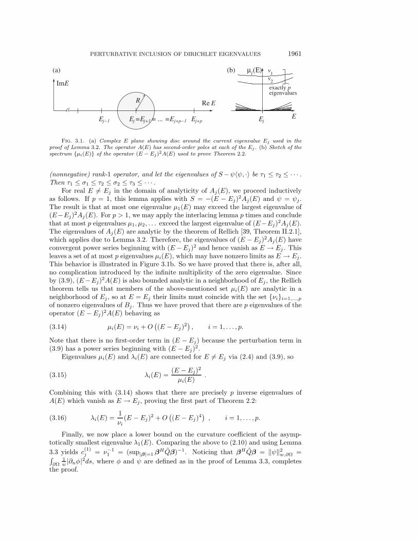
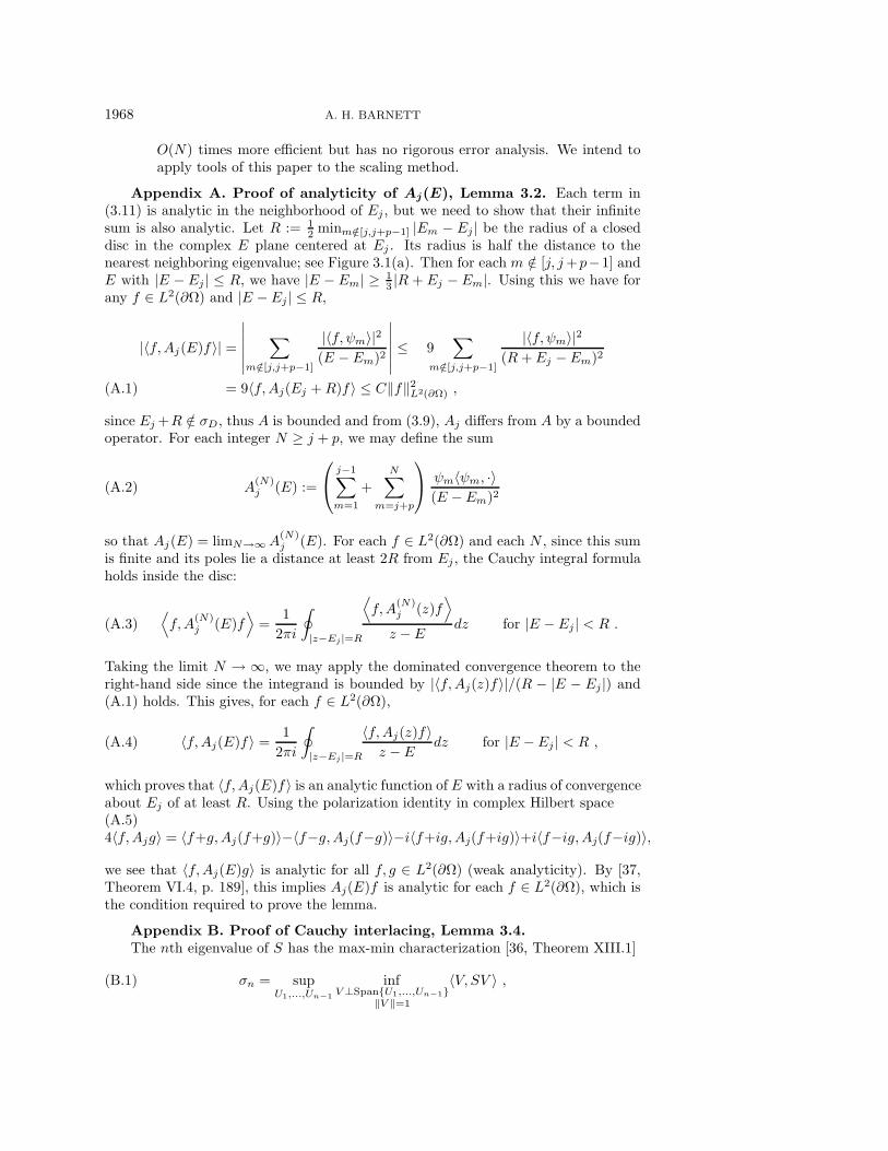
Fig. 3.1. (a) Complex E plane showing disc around the current eigenvalue Ej used in theproof of Lemma 3.2. The operator A(E) has second-order poles at each of the Ej. (b) Sketch of thespectrum {μi(E)} of the operator (E − Ej)

2A(E) used to prove Theorem 2.2.

(nonnegative) rank-1 operator, and let the eigenvalues of S−ψ〈ψ, ·〉 be τ1 ≤ τ2 ≤ · · · .Then τ1 ≤ σ1 ≤ τ2 ≤ σ2 ≤ τ3 ≤ · · · .

For real E �= Ej in the domain of analyticity of Aj(E), we proceed inductivelyas follows. If p = 1, this lemma applies with S = −(E − Ej)2Aj(E) and ψ = ψj .The result is that at most one eigenvalue μ1(E) may exceed the largest eigenvalue of(E−Ej)2Aj(E). For p > 1, we may apply the interlacing lemma p times and concludethat at most p eigenvalues μ1, μ2, . . . exceed the largest eigenvalue of (E−Ej)2Aj(E).The eigenvalues of Aj(E) are analytic by the theorem of Rellich [39, Theorem II.2.1],which applies due to Lemma 3.2. Therefore, the eigenvalues of (E −Ej)2Aj(E) haveconvergent power series beginning with (E−Ej)2 and hence vanish as E → Ej . Thisleaves a set of at most p eigenvalues μi(E), which may have nonzero limits as E → Ej .This behavior is illustrated in Figure 3.1b. So we have proved that there is, after all,no complication introduced by the infinite multiplicity of the zero eigenvalue. Sinceby (3.9), (E−Ej)2A(E) is also bounded analytic in a neighborhood of Ej , the Rellichtheorem tells us that members of the above-mentioned set μi(E) are analytic in aneighborhood of Ej , so at E = Ej their limits must coincide with the set {νi}i=1,...,p

of nonzero eigenvalues of Bj . Thus we have proved that there are p eigenvalues of theoperator (E − Ej)2A(E) behaving as

(3.14) μi(E) = νi +O((E − Ej)2

), i = 1, . . . , p.

Note that there is no first-order term in (E − Ej) because the perturbation term in(3.9) has a power series beginning with (E − Ej)2.

Eigenvalues μi(E) and λi(E) are connected for E �= Ej via (2.4) and (3.9), so

(3.15) λi(E) =(E − Ej)2

μi(E).

Combining this with (3.14) shows that there are precisely p inverse eigenvalues ofA(E) which vanish as E → Ej , proving the first part of Theorem 2.2:

(3.16) λi(E) =1νi

(E − Ej)2 +O((E − Ej)4

), i = 1, . . . , p.

Finally, we now place a lower bound on the curvature coefficient of the asymp-totically smallest eigenvalue λ1(E). Comparing the above to (2.10) and using Lemma3.3 yields c(1)j = ν−1

1 = (sup|β|=1 βHQβ)−1. Noticing that βHQβ = ‖ψ‖2w,∂Ω =∫

∂Ω1w |∂nφ|2ds, where φ and ψ are defined as in the proof of Lemma 3.3, completes

the proof.

1962 A. H. BARNETT

4. Implementation and performance of eigenvalue inclusion. Here wediscuss an efficient two-dimensional (d = 2) implementation of the MPS, then showthat, in practice, Theorem 1.1 gives useful eigenvalue inclusion bounds even for εmuch smaller than 1. As illustrated in Figure 1.1, these supercede the Moler–Paynebounds.

4.1. Computation of minimum boundary error tm(E). At each given fre-quency E, inserting the basis representation u =

∑Nn=1 αnξn converts the minimum

boundary error (1.5) into the Rayleigh quotient (here, α := (α1, . . . , αN )T and H

indicates conjugate transpose)

(4.1) tm(E) = minu∈Span{ξn}

‖u‖w,∂Ω

‖u‖Ω= min

α=0

√αHF (E)ααHG(E)α

=√λ1(E) ,

where λ1(E) is the smallest generalized eigenvalue of the matrix pencil defined by

(4.2) Fα = λGα .

Note that here, and from now on, we use the weighted boundary norm (1.7) in placeof ‖u‖∂Ω. The matrix elements are (for m,n = 1, . . . , N)

(4.3) Fmn(E) :=∫∂Ω

w(s)ξm(s)ξn(s) ds , Gmn(E) := (ξm, ξn)Ω .

With a good choice of basis set (e.g., see section 4.2), λ1(E) is very close to itsminimum achievable value λ1(E).

We now discuss how we fill F and G efficiently, which is not trivial at highfrequency. Naively, we might expect that N2 separate boundary integrals are requiredto fill F , where N is the basis size. As we discuss below (and in [2]) to achievereasonable approximations of eigenmodes, N must scale like

√E at high frequency.

Each such integral must be approximated using a set of M quadrature points xi ∈ ∂Ω.Since integrands oscillate on the wavelength scale, it turns out that M must also scalelike

√E, so M is the same order as N . Thus O(N3) basis function evaluations would

be required to fill F . However, we can reduce this to O(N2) by writing F ≈ AHWA,where the M × N rectangular matrix A has elements Ain(E) := ξn(xi) and W is adiagonal matrix containing the products of w(xi) and the quadrature weights. Thedense matrix-matrix product remains O(N3), but now the prefactor is much smaller(since basis functions are typically trigonometric or Bessels and may require 102 flopsor more per evaluation).

The naive cost of filling G is worse: each domain integral would require O(N2)quadrature points to handle the oscillatory integrand; even using the factorizationabove would bring this only down to O(N3) basis evaluations. However, we maymake use of the following identity [4, Lemma 3.1] (also see [3, Appendix H]). Let−Δu = Eu and −Δv = Ev hold in any Lipschitz domain Ω ∈ R2, then

(4.4) (u, v)Ω =1

2E

∫∂Ω

(x ·n)(Euv−∇u ·∇v)+ (x ·∇u)(n ·∇v)+ (n ·∇u)(x ·∇v) ds

expresses the domain inner product as a sum of four boundary inner products. Sub-stituting this into (4.3) using u = ξm and v = ξn, we see that G can be written asa sum of four boundary integral matrices of similar form to F . By computing each

PERTURBATIVE INCLUSION OF DIRICHLET EIGENVALUES 1963

of the four terms using a product of rectangular matrices as with F , we may, there-fore, fill G using only O(N2) basis (and first-derivative) evaluations plus a few densematrix-matrix products which are O(N3) with a small prefactor.

Solving the generalized eigenvalue problem (4.2) has an interesting twist: it turnsout to become numerically singular, with F and G effectively acquiring a commonnullspace whenever N is chosen large enough to achieve high accuracy. This is due tothe fact that as N increases, there arise unit-norm linear combinations of basis func-tions which have exponentially small values in the closure of Ω; this ill-conditioning ofthe basis appears to be a general feature of MPS type methods [12, 5, 2]. As a conse-quence, standard methods, such as Cholesky factorization of the (formally) positive-definite matrix G [20, section 8.7] or QZ decomposition [20, section 7.7], do notproduce reliable eigenvalues of (4.2).2 However, by using the following regularizationmethod, we project out the numerical nullspace and accurately compute the remaining“stable” (in the sense of [15]) eigenvalues. We diagonalize the Hermitian matrix G =V DV H (where V is unitary), then define D to be the diagonal matrix containing onlythe subset of entries of D which exceed a cutoff εreg (typically 10−15) times D’s largestentry. Defining V to contain as columns the corresponding subset of eigenvectors and

(4.5) F := D−1/2V HFV D−1/2 ,

we diagonalize F = UΛUH . The diagonal matrix Λ contains approximations to thestable eigenvalues λ of the pencil (4.2), with eigenvectors as the columns of V D−1/2U .

The above method was used by Vergini–Saraceno [46] and is similar to a moregeneral procedure of Fix–Heiberger [15], who show that the error introduced into thestable eigenvalues is O(εreg). In practice, we find that the errors are bounded byroughly 103εreg. We believe that this prefactor reflects the closeness of the nullspacesof F and G; however, this method deserves a full analysis, which we will not attempthere. We also find (by extrapolating in εreg) that the approximate λ1 overestimatesthe true value. Note that Betcke’s recent GSVD method [7] includes a regularizationsimilar to the above and can give higher accuracy; we discuss this in comment 2 ofsection 5. Finally, since only the lowest (or lowest few) eigenvalues are needed, onemight expect that an iterative method could improve upon the above O(N3) effort.

4.2. Testing the applicability of the main theorem. Theorem 1.1 is anasymptotic result: given an ε > 0, it does not tell us in how large a (punctured)neighborhood of each Ej the inequality (1.6) holds, only that some neighborhoodexists. We now show that, in practice, for a small choice of ε, the valid neighborhoodsaround each Ej coalesce so that the theorem may be applied to essentially the wholepositive real axis, i.e., Σε = [a,∞) for some small a. Our three test domains aredefined and shown in Figure 1.2 and represent three classes of interest: (S) is smooth,(T) is a triangle with one singular (5π/12) corner, and (H) is a “horseshoe” with C1

continuous boundary. Recall that a singular corner is a corner with angle not equalto π/n for some n ∈ N [5]. (S) and (T) are strictly star-shaped, but (H) is not.

Before presenting results, we discuss implementation details. To compute tm(E),we used the method of the previous section. For (S) and (H), we use as basis functionsξn fundamental solutions with origins (source points) placed along an exterior curvea distance of order one wavelength from Ω. Such bases are efficient in many domains[14, 12] and show spectral convergence in analytic domains [2]. For (T), we use acylindrical wave expansion (generalized harmonic polynomials), in polar coordinates

2We implement these with the eig command of MATLAB version 2007b.

1964 A. H. BARNETT

0 200 400 600 800 10000

0.2

0.4

0.6

0.8

1

E

f

(a)

0 200 400 600 800 1000

10−6

10−4

10−2

f−1

E

(b)

Fig. 4.1. (a) Relative slope measure f(E) defined by (4.6), for the smooth domain (S) withweight w = (x · n)−1, plotted at E = 5, 6, 7, . . . , 1000. (b) Logarithmic plot of f(E) − 1 (no point isplotted if f(E) < 1). The value f(E)−1 is the smallest value of ε in Theorem 1.1 such that E ∈ Σε.

ξn(r, θ) = einθJn(√Er) for −N/2 ≤ n < N/2 and N even. This basis is convergent

in any bounded Ω with a finite number of corners [41, Corollary to Theorem I6.1]. Itis extremely fast to evaluate (at each r, all n values may be computed via a singleMiller’s downward recurrence [35, section 5.4]), and we found that it produced valuesof tm(E) for E = Ej , j < 103, no larger than 10−3, adequate for our needs. (Notethat this could be improved upon by adding functions adapted to the singular corner[10, 5].) In all three domains the scaling of basis size with wavenumber was linear: wetypically chose between 3 to 6 degrees of freedom per wavelength on the boundary.Boundary quadrature was equispaced in angle for (S), and Clenshaw–Curtis [44] oneach side of (T) and each arc of (H). In all cases, the number of quadrature points Mwas chosen to be large enough to make the results insensitive to M (as discussed in[2]); generally, M was between N and 2N . For (S) and (T), Dirichlet eigenvalues Ejwere independently located with the scaling method [46, 3, 4] to an absolute error ofroughly 10−3; for (H), these were located by finding minima of tm(E). In all cases,the first two terms of Weyl’s law for the asymptotics of eigenvalues [22] was used toeliminate the possibility of missing eigenvalues.

Motivated by (1.6), given some constant CΩ, we will study the “relative slopemeasure”

(4.6) f(E) :=1

CΩtm(E)minj

|E − Ej |√Ej

.

The interpretation is that f(E)− 1 gives a strict lower bound on ε such that E ∈ Σε.A value of f close to 1 shows that the perturbative result Theorem 2.2 that we usedto prove Theorem 1.1 is accurately predicting the slopes in curves such as Figure 1.1.

We start with domain (S), and choose w = (x · n)−1, thus use CΩ =√

2. InFigure 4.1 we show f(E) computed at E = 5, 6, 7, . . . , 1000. Note that the lowest 242Dirichlet eigenvalues Ej lie in the interval [5, 1000] and have no known correlation withthe integers (we have checked that random sampling of E gives the same behavior).It is clear that f is almost always close to 1, in fact, the largest value is f(9) = 1.0335.Panel (b) shows the overall tendency that f values approach 1 from above as E grows.Occasionally, f values are significantly smaller than 1: this happens only when E isvery close to Ej for some j and limitations of the basis set prevent tm(E) from reachingits theoretical minimum. Occasionally there is an anomalously large f value at higherE: in all cases these spikes in f(E) occur for E very close to Ej for some j and aredue to the errors in the computed Ej . For instance, the largest such value shown is

PERTURBATIVE INCLUSION OF DIRICHLET EIGENVALUES 1965

0 2000 4000 60000

0.2

0.4

0.6

0.8

1

E

f

(a)

0 2000 4000 6000

10−6

10−4

10−2

f−1

E

(b)

0 200 400 6000

0.2

0.4

0.6

0.8

1

E

f

(c)

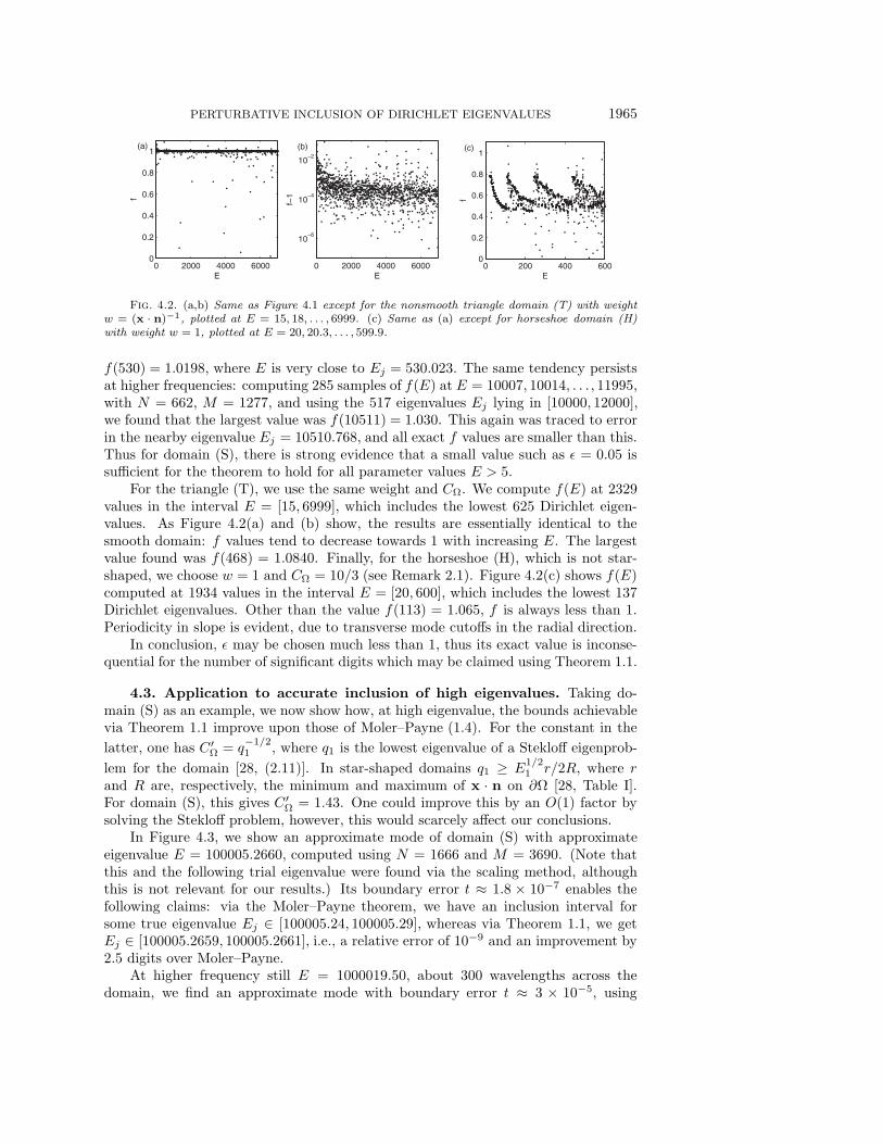
Fig. 4.2. (a,b) Same as Figure 4.1 except for the nonsmooth triangle domain (T) with weightw = (x · n)−1, plotted at E = 15, 18, . . . , 6999. (c) Same as (a) except for horseshoe domain (H)with weight w = 1, plotted at E = 20, 20.3, . . . , 599.9.

f(530) = 1.0198, where E is very close to Ej = 530.023. The same tendency persistsat higher frequencies: computing 285 samples of f(E) at E = 10007, 10014, . . . , 11995,with N = 662, M = 1277, and using the 517 eigenvalues Ej lying in [10000, 12000],we found that the largest value was f(10511) = 1.030. This again was traced to errorin the nearby eigenvalue Ej = 10510.768, and all exact f values are smaller than this.Thus for domain (S), there is strong evidence that a small value such as ε = 0.05 issufficient for the theorem to hold for all parameter values E > 5.

For the triangle (T), we use the same weight and CΩ. We compute f(E) at 2329values in the interval E = [15, 6999], which includes the lowest 625 Dirichlet eigen-values. As Figure 4.2(a) and (b) show, the results are essentially identical to thesmooth domain: f values tend to decrease towards 1 with increasing E. The largestvalue found was f(468) = 1.0840. Finally, for the horseshoe (H), which is not star-shaped, we choose w = 1 and CΩ = 10/3 (see Remark 2.1). Figure 4.2(c) shows f(E)computed at 1934 values in the interval E = [20, 600], which includes the lowest 137Dirichlet eigenvalues. Other than the value f(113) = 1.065, f is always less than 1.Periodicity in slope is evident, due to transverse mode cutoffs in the radial direction.

In conclusion, ε may be chosen much less than 1, thus its exact value is inconse-quential for the number of significant digits which may be claimed using Theorem 1.1.

4.3. Application to accurate inclusion of high eigenvalues. Taking do-main (S) as an example, we now show how, at high eigenvalue, the bounds achievablevia Theorem 1.1 improve upon those of Moler–Payne (1.4). For the constant in thelatter, one has C′

Ω = q−1/21 , where q1 is the lowest eigenvalue of a Stekloff eigenprob-

lem for the domain [28, (2.11)]. In star-shaped domains q1 ≥ E1/21 r/2R, where r

and R are, respectively, the minimum and maximum of x · n on ∂Ω [28, Table I].For domain (S), this gives C′

Ω = 1.43. One could improve this by an O(1) factor bysolving the Stekloff problem, however, this would scarcely affect our conclusions.

In Figure 4.3, we show an approximate mode of domain (S) with approximateeigenvalue E = 100005.2660, computed using N = 1666 and M = 3690. (Note thatthis and the following trial eigenvalue were found via the scaling method, althoughthis is not relevant for our results.) Its boundary error t ≈ 1.8 × 10−7 enables thefollowing claims: via the Moler–Payne theorem, we have an inclusion interval forsome true eigenvalue Ej ∈ [100005.24, 100005.29], whereas via Theorem 1.1, we getEj ∈ [100005.2659, 100005.2661], i.e., a relative error of 10−9 and an improvement by2.5 digits over Moler–Payne.

At higher frequency still E = 1000019.50, about 300 wavelengths across thedomain, we find an approximate mode with boundary error t ≈ 3 × 10−5, using

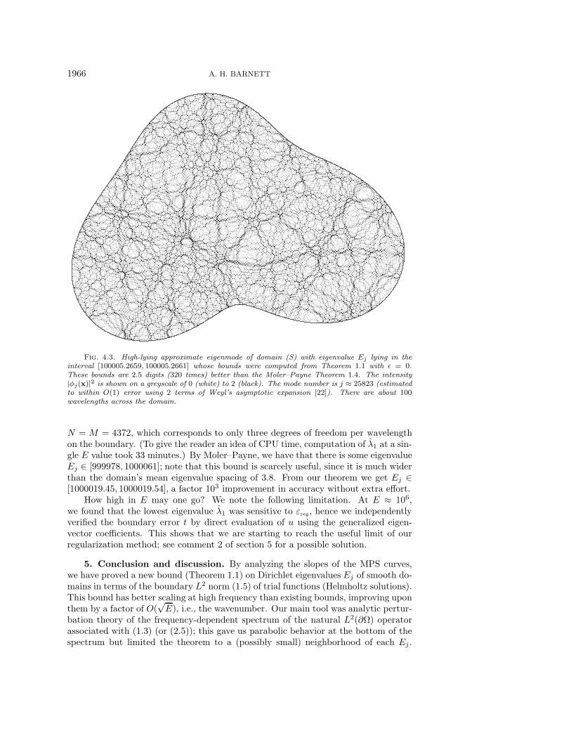
1966 A. H. BARNETT

Fig. 4.3. High-lying approximate eigenmode of domain (S) with eigenvalue Ej lying in theinterval [100005.2659, 100005.2661] whose bounds were computed from Theorem 1.1 with ε = 0.These bounds are 2.5 digits (320 times) better than the Moler–Payne Theorem 1.4. The intensity|φj(x)|2 is shown on a greyscale of 0 (white) to 2 (black). The mode number is j ≈ 25823 (estimatedto within O(1) error using 2 terms of Weyl’s asymptotic expansion [22]). There are about 100wavelengths across the domain.

N = M = 4372, which corresponds to only three degrees of freedom per wavelengthon the boundary. (To give the reader an idea of CPU time, computation of λ1 at a sin-gle E value took 33 minutes.) By Moler–Payne, we have that there is some eigenvalueEj ∈ [999978, 1000061]; note that this bound is scarcely useful, since it is much widerthan the domain’s mean eigenvalue spacing of 3.8. From our theorem we get Ej ∈[1000019.45, 1000019.54], a factor 103 improvement in accuracy without extra effort.

How high in E may one go? We note the following limitation. At E ≈ 106,we found that the lowest eigenvalue λ1 was sensitive to εreg, hence we independentlyverified the boundary error t by direct evaluation of u using the generalized eigen-vector coefficients. This shows that we are starting to reach the useful limit of ourregularization method; see comment 2 of section 5 for a possible solution.

5. Conclusion and discussion. By analyzing the slopes of the MPS curves,we have proved a new bound (Theorem 1.1) on Dirichlet eigenvalues Ej of smooth do-mains in terms of the boundary L2 norm (1.5) of trial functions (Helmholtz solutions).This bound has better scaling at high frequency than existing bounds, improving uponthem by a factor of O(

√E), i.e., the wavenumber. Our main tool was analytic pertur-

bation theory of the frequency-dependent spectrum of the natural L2(∂Ω) operatorassociated with (1.3) (or (2.5)); this gave us parabolic behavior at the bottom of thespectrum but limited the theorem to a (possibly small) neighborhood of each Ej .

PERTURBATIVE INCLUSION OF DIRICHLET EIGENVALUES 1967

250 260 270 280 290 300 310 320 330 340 3500

0.2

0.4

0.6

λ j1/2

(a)w ≡ 1

250 260 270 280 290 300 310 320 330 340 3500

0.2

0.4

E

λ j1/2

(b)w = ( x.n)−1

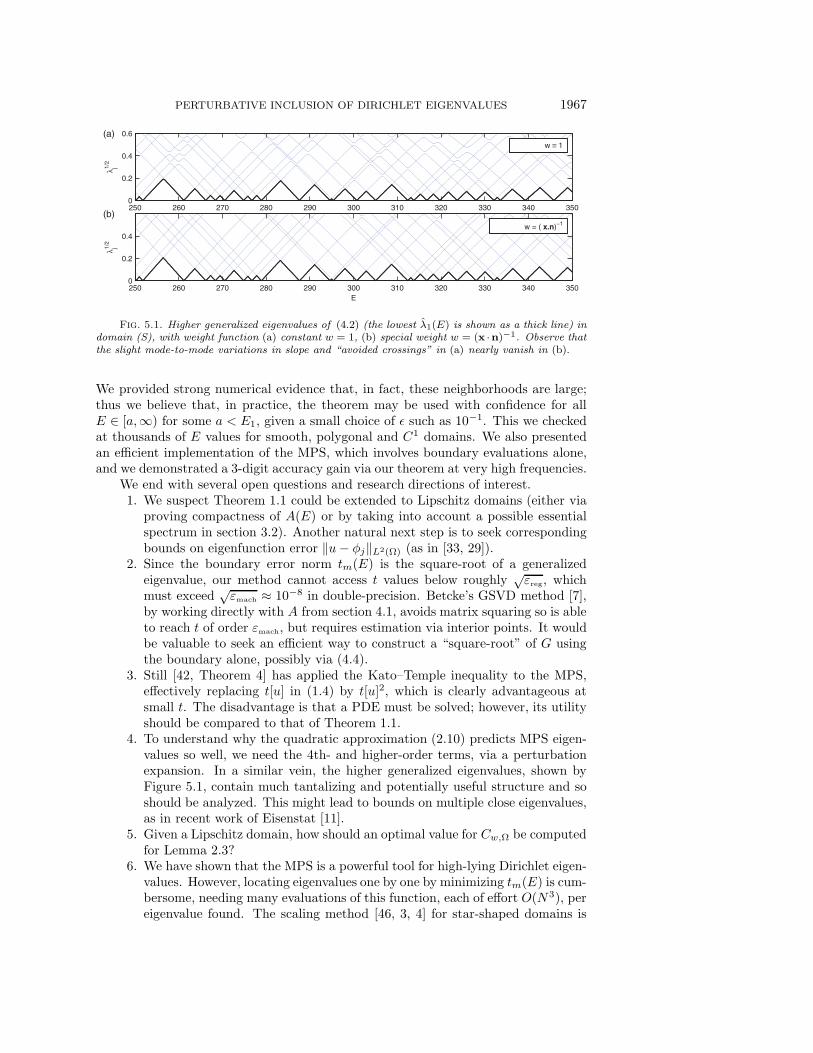
Fig. 5.1. Higher generalized eigenvalues of (4.2) (the lowest λ1(E) is shown as a thick line) indomain (S), with weight function (a) constant w = 1, (b) special weight w = (x ·n)−1. Observe thatthe slight mode-to-mode variations in slope and “avoided crossings” in (a) nearly vanish in (b).

We provided strong numerical evidence that, in fact, these neighborhoods are large;thus we believe that, in practice, the theorem may be used with confidence for allE ∈ [a,∞) for some a < E1, given a small choice of ε such as 10−1. This we checkedat thousands of E values for smooth, polygonal and C1 domains. We also presentedan efficient implementation of the MPS, which involves boundary evaluations alone,and we demonstrated a 3-digit accuracy gain via our theorem at very high frequencies.

We end with several open questions and research directions of interest.1. We suspect Theorem 1.1 could be extended to Lipschitz domains (either via

proving compactness of A(E) or by taking into account a possible essentialspectrum in section 3.2). Another natural next step is to seek correspondingbounds on eigenfunction error ‖u− φj‖L2(Ω) (as in [33, 29]).

2. Since the boundary error norm tm(E) is the square-root of a generalizedeigenvalue, our method cannot access t values below roughly √

εreg, whichmust exceed

√εmach ≈ 10−8 in double-precision. Betcke’s GSVD method [7],

by working directly with A from section 4.1, avoids matrix squaring so is ableto reach t of order εmach, but requires estimation via interior points. It wouldbe valuable to seek an efficient way to construct a “square-root” of G usingthe boundary alone, possibly via (4.4).

3. Still [42, Theorem 4] has applied the Kato–Temple inequality to the MPS,effectively replacing t[u] in (1.4) by t[u]2, which is clearly advantageous atsmall t. The disadvantage is that a PDE must be solved; however, its utilityshould be compared to that of Theorem 1.1.

4. To understand why the quadratic approximation (2.10) predicts MPS eigen-values so well, we need the 4th- and higher-order terms, via a perturbationexpansion. In a similar vein, the higher generalized eigenvalues, shown byFigure 5.1, contain much tantalizing and potentially useful structure and soshould be analyzed. This might lead to bounds on multiple close eigenvalues,as in recent work of Eisenstat [11].

5. Given a Lipschitz domain, how should an optimal value for Cw,Ω be computedfor Lemma 2.3?

6. We have shown that the MPS is a powerful tool for high-lying Dirichlet eigen-values. However, locating eigenvalues one by one by minimizing tm(E) is cum-bersome, needing many evaluations of this function, each of effort O(N3), pereigenvalue found. The scaling method [46, 3, 4] for star-shaped domains is

1968 A. H. BARNETT

O(N) times more efficient but has no rigorous error analysis. We intend toapply tools of this paper to the scaling method.

Appendix A. Proof of analyticity of Aj(E), Lemma 3.2. Each term in(3.11) is analytic in the neighborhood of Ej , but we need to show that their infinitesum is also analytic. Let R := 1

2 minm/∈[j,j+p−1] |Em − Ej | be the radius of a closeddisc in the complex E plane centered at Ej . Its radius is half the distance to thenearest neighboring eigenvalue; see Figure 3.1(a). Then for each m /∈ [j, j+p−1] andE with |E − Ej | ≤ R, we have |E − Em| ≥ 1

3 |R + Ej − Em|. Using this we have forany f ∈ L2(∂Ω) and |E − Ej | ≤ R,

|〈f,Aj(E)f〉| =

∣∣∣∣∣∣∑

m/∈[j,j+p−1]

|〈f, ψm〉|2(E − Em)2

∣∣∣∣∣∣ ≤ 9∑

m/∈[j,j+p−1]

|〈f, ψm〉|2(R+ Ej − Em)2

= 9〈f,Aj(Ej +R)f〉 ≤ C‖f‖2L2(∂Ω) ,(A.1)

since Ej +R /∈ σD, thus A is bounded and from (3.9), Aj differs from A by a boundedoperator. For each integer N ≥ j + p, we may define the sum

(A.2) A(N)j (E) :=

⎛⎝ j−1∑m=1

+N∑

m=j+p

⎞⎠ ψm〈ψm, ·〉

(E − Em)2

so that Aj(E) = limN→∞A(N)j (E). For each f ∈ L2(∂Ω) and each N , since this sum

is finite and its poles lie a distance at least 2R from Ej , the Cauchy integral formulaholds inside the disc:

(A.3)⟨f,A

(N)j (E)f

⟩=

12πi

∮|z−Ej|=R

⟨f,A

(N)j (z)f

⟩z − E

dz for |E − Ej | < R .

Taking the limit N → ∞, we may apply the dominated convergence theorem to theright-hand side since the integrand is bounded by |〈f,Aj(z)f〉|/(R − |E − Ej |) and(A.1) holds. This gives, for each f ∈ L2(∂Ω),

(A.4) 〈f,Aj(E)f〉 =1

2πi

∮|z−Ej|=R

〈f,Aj(z)f〉z − E

dz for |E − Ej | < R ,

which proves that 〈f,Aj(E)f〉 is an analytic function of E with a radius of convergenceabout Ej of at least R. Using the polarization identity in complex Hilbert space(A.5)4〈f,Ajg〉 = 〈f+g,Aj(f+g)〉−〈f−g,Aj(f−g)〉−i〈f+ig, Aj(f+ig)〉+i〈f−ig, Aj(f−ig)〉,

we see that 〈f,Aj(E)g〉 is analytic for all f, g ∈ L2(∂Ω) (weak analyticity). By [37,Theorem VI.4, p. 189], this implies Aj(E)f is analytic for each f ∈ L2(∂Ω), which isthe condition required to prove the lemma.

Appendix B. Proof of Cauchy interlacing, Lemma 3.4.The nth eigenvalue of S has the max-min characterization [36, Theorem XIII.1]

(B.1) σn = supU1,...,Un−1

infV⊥Span{U1,...,Un−1}

‖V ‖=1

〈V, SV 〉 ,

PERTURBATIVE INCLUSION OF DIRICHLET EIGENVALUES 1969

where the sup is over all possible sets of n − 1 vectors in the Hilbert space. Theanalogous formula for τn is found by replacing S with R := S − ψ〈ψ, ·〉. Since for allV ∈ L2(∂Ω) it holds that 〈V,RV 〉 = 〈V, SV 〉 − |〈V, ψ〉|2 ≤ 〈V, SV 〉, the same holdsfor the max-min values, hence for each n = 1, 2, . . . , we have τn ≤ σn. In addition,using (B.1) we have the inequalities

σn ≤ supU1,...,Un−1

infV⊥Span{U1,...,Un−1,ψ}

‖V ‖=1

〈V, SV 〉

= supU1,...,Un−1

infV⊥Span{U1,...,Un−1,ψ}

‖V ‖=1

〈V,RV 〉

≤ supU1,...,Un

infV⊥Span{U1,...,Un}

‖V ‖=1

〈V,RV 〉 = τn+1 .

The middle equality follows since V is orthogonal to ψ; the inequalities are standardlinear subspace arguments. Thus the interlacing τn ≤ σn ≤ τn+1 is proved.

Acknowledgments. The author is indebted to Percy Deift and Jonathan Good-man for introducing many of the ideas which made this work possible. The author alsothanks Ross Barnett, Timo Betcke, Leslie Greengard, Andrew Hassell, Chris Judge,Bob Kohn, Peter Lax, Kevin Lin, Mikhail Shubin, Nick Trefethen, Eduardo Vergini,and the referees for useful input.

REFERENCES

[1] A. Backer, Numerical aspects of eigenvalue and eigenfunction computations for chaotic quan-tum systems, in The Mathematical Aspects of Quantum Maps, Lect. Notes Phys. 618,Springer, Berlin, 2003, pp. 91–144.

[2] A. H. Barnett and T. Betcke, Stability and convergence of the method of fundamentalsolutions for Helmholtz problems on analytic domains, J. Comput. Phys., 227 (2008),pp. 7003–7026.

[3] A. H. Barnett, Dissipation in Deforming Chaotic Billiards, Ph.D. thesis, Harvard University,Cambridge, MA, 2000, http://www.math.dartmouth.edu/˜ahb/thesis html/.

[4] A. H. Barnett, Asymptotic rate of quantum ergodicity in chaotic Euclidean billiards, Comm.Pure Appl. Math., 59 (2006), pp. 1457–88.

[5] T. Betcke and L. N. Trefethen, Reviving the method of particular solutions, SIAM Rev.,47 (2005), pp. 469–491.

[6] T. Betcke, A GSVD formulation of a domain decomposition method for planar eigenvalueproblems, IMA J. Numer. Anal., 27 (2007), pp. 451–478.

[7] T. Betcke, The generalized singular value decomposition and the method of particular solu-tions, SIAM J. Sci. Comput., 30 (2008), pp. 1278–1295.

[8] J. Descloux and M. Tolley, An accurate algorithm for computing the eigenvalues of apolygonal membrane, Comput. Methods Appl. Mech. Engrg., 39 (1983), pp. 37–53.

[9] T. A. Driscoll, Eigenmodes of isospectral drums, SIAM Rev., 39 (1997), pp. 1–17.[10] S. C. Eisenstat, On the rate of convergence of the Bergman–Vekua method for the numerical

solution of elliptic boundary value problems, SIAM J. Numer. Anal., 11 (1974), pp. 654–680.

[11] S. C. Eisenstat, Bounds for Eigenvalues and Eigenvectors of Self-adjoint Operators, preprint,2006.

[12] R. Ennenbach and H. Niemeyer, The inclusion of Dirichlet eigenvalues with singularityfunctions, Z. Angew. Math. Mech., 76 (1996), pp. 377–383.

[13] L. C. Evans, Partial Differential Equations, Grad. Stud. Math. 19, American MathematicalSociety, Providence, RI, 1998.

[14] G. Fairweather and A. Karageorghis, The method of fundamental solutions for ellipticboundary value problems, Adv. Comput. Math., 9 (1998), pp. 69–95.

[15] G. Fix and R. Heiberger, An algorithm for the ill-conditioned generalized eigenvalue problem,SIAM J. Numer. Anal., 9 (1972), pp. 78–88.

1970 A. H. BARNETT

[16] L. Fox, P. Henrici, and C. Moler, Approximations and bounds for eigenvalues of ellipticoperators, SIAM J. Numer. Anal., 4 (1967), pp. 89–102.

[17] L. Friedlander, Some inequalities between Dirichlet and Neumann eigenvalues, Arch. Ration.Mech. Anal., 116 (1991), pp. 153–160.

[18] P. R. Garabedian, Partial Differential Equations, John Wiley & Sons, New York, 1964.[19] P. Gerard and E. Leichtnam, Ergodic properties of eigenfunctions for the Dirichlet problem,

Duke Math. J., 71 (1993), pp. 559–607.[20] G. H. Golub and C. F. Van Loan, Matrix computations, 3rd ed., Johns Hopkins Studies in

the Mathematical Sciences, Johns Hopkins University Press, Baltimore, MD, 1996.[21] C. Gordon, D. Webb, and S. Wolpert, Isospectral plane domains and surfaces via Rieman-

nian orbifolds, Invent. Math., 110 (1992), pp. 1–22.[22] M. C. Gutzwiller, Chaos in Classical and Quantum Mechanics, Interdiscip. Appl. Math.,

Springer, New York, 1990.[23] A. Hassell, personal communication, 2005.[24] A. Hassell and T. Tao, Upper and lower bounds for normal derivatives of Dirichlet eigen-

functions, Math. Res. Lett., 9 (2002), pp. 289–305.[25] E. J. Heller, Bound-state eigenfunctions of classically chaotic Hamiltonian systems: Scars

of periodic orbits, Phys. Rev. Lett., 53 (1984), pp. 1515–1518.[26] E. J. Heller, Wavepacket dynamics and quantum chaology, in Chaos et Physique Quantique

(Les Houches, 1989), North-Holland, Amsterdam, 1991, pp. 547–664.[27] A. Karageorghis, The method of fundamental solutions for the calculation of the eigenvalues

of the Helmholtz equation, Appl. Math. Lett., 14 (2001), pp. 837–842.[28] J. R. Kuttler and V. G. Sigillito, Inequalities for membrane and Stekloff eigenvalues, J.

Math. Anal. Appl., 23 (1968), pp. 148–160.[29] J. R. Kuttler and V. G. Sigillito, Bounding eigenvalues of elliptic operators, SIAM J.

Math. Anal., 9 (1978), pp. 768–778.[30] J. R. Kuttler and V. G. Sigillito, Eigenvalues of the Laplacian in two dimensions, SIAM

Rev., 26 (1984), pp. 163–193.[31] J.-L. Lions and E. Magenes, Problemes aux limites non homogenes et applications, Vol. 3,

Dunod, Paris, 1970. Travaux et Recherches Mathematiques, 20.[32] W. C. H. McLean, Strongly Elliptic Systems and Boundary Integral Equations, Cambridge

University Press, London, 2000.[33] C. B. Moler and L. E. Payne, Bounds for eigenvalues and eigenvectors of symmetric opera-

tors, SIAM J. Numer. Anal., 5 (1968), pp. 64–70.[34] A. Nachman, J. Sylvester, and G. Uhlmann, An n-dimensional Borg-Levinson theorem,

Comm. Math. Phys., 115 (1988), pp. 595–605.[35] W. H. Press, S. A. Teukolsky, W. T. Vetterling, and B. P. Flannery, Numerical Recipes

in C, 2nd ed., Cambridge University Press, Cambridge, 2002.[36] M. Reed and B. Simon, Methods of Modern Mathematical Physics. IV. Analysis of Operators,

Academic Press, New York, 1978.[37] M. Reed and B. Simon, Methods of Modern Mathematical Physics. I. Functional Analysis,

2nd ed., Academic Press, New York, 1980.[38] F. Rellich, Darstellung der Eigenwerte von Δu + λu = 0 durch ein Randintegral, Math. Z.,

46 (1940), pp. 635–636.[39] F. Rellich, Perturbation Theory of Eigenvalue Problems, Gordon and Breach, New York,

1969.[40] N. Saito, Data analysis and representation on a general domain using eigenfunctions of Lapla-

cian, Appl. Comput. Harmon. Anal., 25 (2008), pp. 68–97.[41] N. L. Schryer, Constructive approximation of solutions to linear elliptic boundary value prob-

lems, SIAM J. Numer. Anal., 9 (1972), pp. 546–572.[42] G. Still, Computable bounds for eigenvalues and eigenfunctions of elliptic differential opera-

tors, Numer. Math., 54 (1988), pp. 201–223.[43] L. N. Trefethen and T. Betcke, Computed eigenmodes of planar regions, Contemp. Math.,

412 (2006), pp. 297–314.[44] L. N. Trefethen, Spectral Methods in MATLAB, Vol. 10, Software, Environments, and Tools,

SIAM, Philadelphia, PA, 2000.[45] H. E. Tureci, H. G. L. Schwefel, P. Jacquod, and A. D. Stone, Modes of wave-chaotic

dielectric resonators, Prog. Optics, 47 (2005), pp. 75–137.[46] E. Vergini and M. Saraceno, Calculation by scaling of highly excited states of billiards, Phys.

Rev. E, 52 (1995), pp. 2204–2207.[47] S. Zelditch, Quantum ergodicity and mixing of eigenfunctions, in Elsevier Encyclopedia of

Mathematical Physics, Vol. 1, Academic Press/Elsevier Science, Oxford, 2006, pp. 183–196,arXiv:math-ph/0503026.